Decision Tree Learning: Part 1

CS 760@UW-Madison

Zoo of machine learning models

Figure from scikit-learn.org

Note: only a subset of ML methods

Even a subarea has its own collection

Figure from asimovinstitute.org

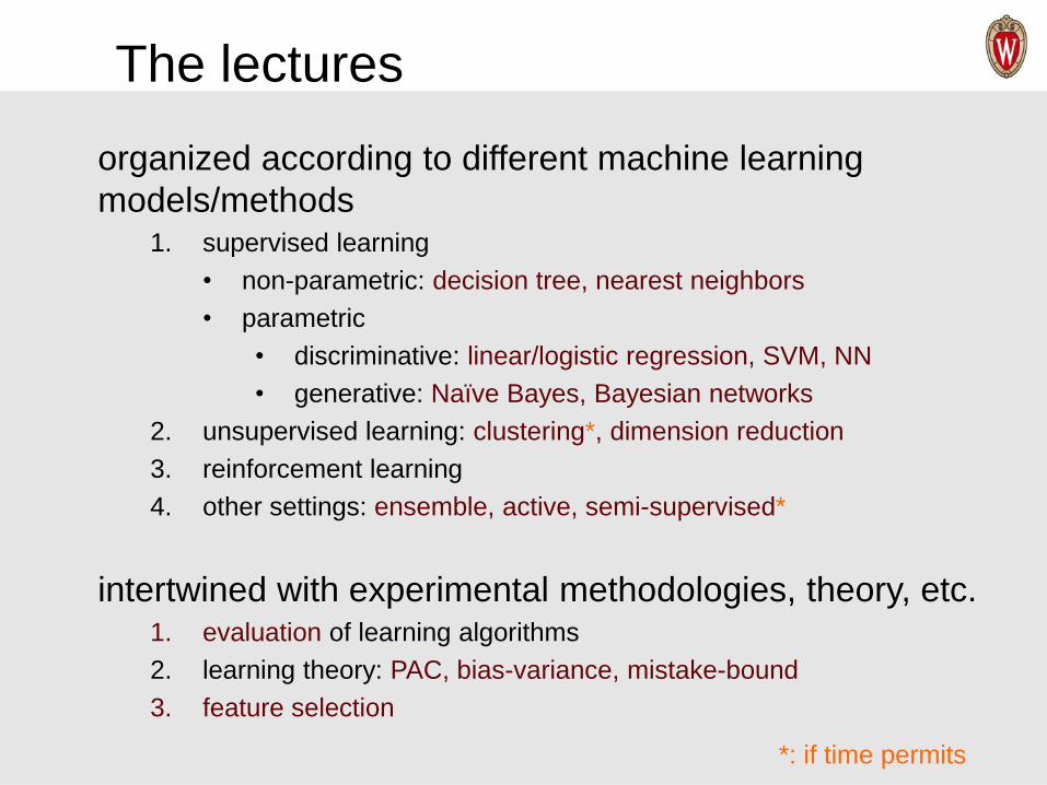
The lectures

organized according to different machine learning

models/methods1. supervised learning

• non-parametric: decision tree, nearest neighbors

• parametric

• discriminative: linear/logistic regression, SVM, NN

• generative: Naïve Bayes, Bayesian networks

2. unsupervised learning: clustering*, dimension reduction

3. reinforcement learning

4. other settings: ensemble, active, semi-supervised*

intertwined with experimental methodologies, theory, etc.1. evaluation of learning algorithms

2. learning theory: PAC, bias-variance, mistake-bound

3. feature selection

*: if time permits

Goals for this lecture

you should understand the following concepts

• the decision tree representation

• the standard top-down approach to learning a tree

• Occam’s razor

• entropy and information gain

Decision Tree Representation

A decision tree to predict heart disease

thal

#_major_vessels > 0 present

normal fixed_defect

true false

1 2

present

reversible_defect

chest_pain_type absent

absentabsentabsent present

3 4

Each internal node tests one feature xi

Each branch from an internal node

represents one outcome of the test

Each leaf predicts y or P(y | x)

Decision tree exercise

Suppose X1 … X5 are Boolean features, and Y is also Boolean

How would you represent the following with decision trees?

) (i.e., 5252 XXYXXY ==

52 XXY =

1352 XXXXY =

Decision Tree Learning

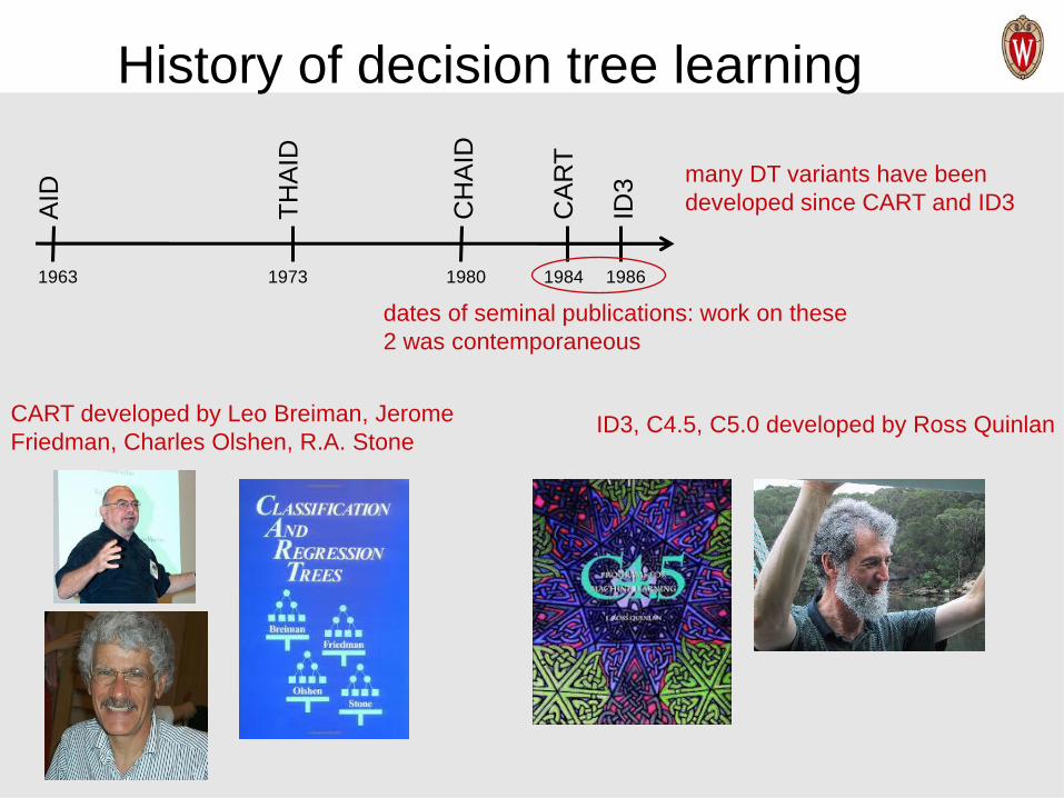
History of decision tree learning

dates of seminal publications: work on these

2 was contemporaneous

many DT variants have been

developed since CART and ID3

1963 1973 1980 1984 1986

AID

CH

AID

TH

AID

CA

RT

ID3

CART developed by Leo Breiman, Jerome

Friedman, Charles Olshen, R.A. StoneID3, C4.5, C5.0 developed by Ross Quinlan

Top-down decision tree learning

MakeSubtree(set of training instances D)

C = DetermineCandidateSplits(D)

if stopping criteria met

make a leaf node N

determine class label/probabilities for N

else

make an internal node N

S = FindBestSplit(D, C)

for each outcome k of S

Dk = subset of instances that have outcome k

kth child of N = MakeSubtree(Dk)

return subtree rooted at N

Candidate splits in ID3, C4.5

• splits on nominal features have one branch per value

• splits on numeric features use a threshold

thal

normal fixed_defect reversible_defect

weight ≤ 35

true false

Candidate splits on numeric features

weight ≤ 35

true false

weight

17 35

given a set of training instances D and a specific feature Xi

• sort the values of Xi in D

• evaluate split thresholds in intervals between instances of different classes

• could use midpoint of each considered interval as the threshold

• C4.5 instead picks the largest value of Xi in the entire training set that does not

exceed the midpoint

Candidate splits on numeric features(in more detail)

// Run this subroutine for each numeric feature at each node of DT induction

DetermineCandidateNumericSplits(set of training instances D, feature Xi)

C = {} // initialize set of candidate splits for feature Xi

S = partition instances in D into sets s1 … sV where the instances in each

set have the same value for Xi

let vj denote the value of Xi for set sj

sort the sets in S using vj as the key for each sj

for each pair of adjacent sets sj, sj+1 in sorted S

if sj and sj+1 contain a pair of instances with different class labels

// assume we’re using midpoints for splits

add candidate split Xi ≤ (vj + vj+1)/2 to C

return C

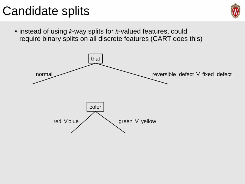
Candidate splits

• instead of using k-way splits for k-valued features, could require binary splits on all discrete features (CART does this)

thal

normal reversible_defect∨ fixed_defect

color

red ∨blue green ∨ yellow

Finding The Best Splits

Finding the best split

• How should we select the best feature to split on at each step?

• Key hypothesis: the simplest tree that classifies the training instances accurately will work well on previously unseen instances

Occam’s razor

• attributed to 14th century William of Ockham

• “Nunquam ponenda est pluralitis sin necesitate”

• “Entities should not be multiplied beyond necessity”

• “when you have two competing theories that make exactly the same

predictions, the simpler one is the better”

But a thousand years earlier,

I said, “We consider it a good

principle to explain the

phenomena by the simplest

hypothesis possible.”

Occam’s razor and decision trees

• there are fewer short models (i.e. small trees) than long ones

• a short model is unlikely to fit the training data well by chance

• a long model is more likely to fit the training data well coincidentally

Why is Occam’s razor a reasonable heuristic for

decision tree learning?

Finding the best splits

• Can we find and return the smallest possible decision tree that accurately classifies the training set?

• Instead, we’ll use an information-theoretic heuristic to

greedily choose splits

NO! This is an NP-hard problem

[Hyafil & Rivest, Information Processing Letters, 1976]

Information theory background

• consider a problem in which you are using a code to communicate information to a receiver

• example: as bikes go past, you are communicating the manufacturer of each bike

Information theory background

• suppose there are only four types of bikes

• we could use the following code

11

10

01

00

• expected number of bits we have to communicate: 2 bits/bike

Trek

Specialized

Cervelo

Serrota

type code

Information theory background

• we can do better if the bike types aren’t equiprobable

• optimal code uses bits for event with probability

- log2 P(y)P(y)

1

 

P(Trek) = 0.5

P(Specialized) = 0.25

P(Cervelo) = 0.125

P(Serrota) = 0.125

2

3

3

1

01

001

000

Type/probability # bits code

• expected number of bits we have to communicate: 1.75 bits/bike

−)(values

2 )(log)(Yy

yPyP

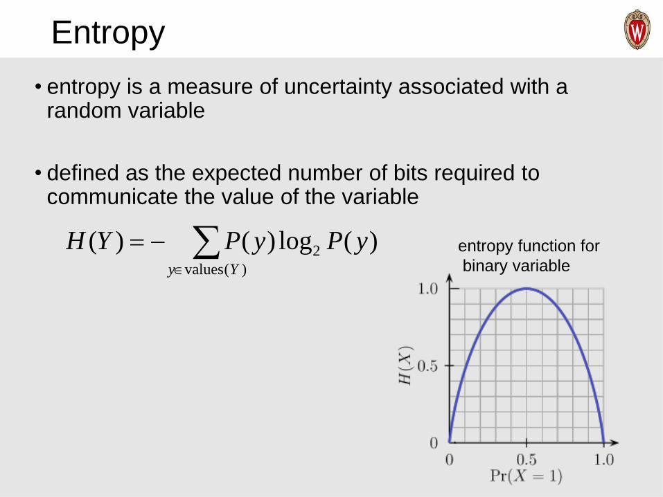
Entropy

• entropy is a measure of uncertainty associated with a random variable

• defined as the expected number of bits required to communicate the value of the variable

entropy function for

binary variable

−=)(values

2 )(log)()(Yy

yPyPYH

Conditional entropy

• What’s the entropy of Y if we condition on some other variable X?

where

𝐻(𝑌|𝑋) =

𝑥∈values(𝑋)

𝑃(𝑋 = 𝑥)𝐻(𝑌|𝑋 = 𝑥)

𝐻(𝑌|𝑋 = 𝑥) = −

𝑦∈values(𝑌)

𝑃(𝑌 = 𝑦|𝑋 = 𝑥) log2 𝑃 (𝑌 = 𝑦|𝑋 = 𝑥)

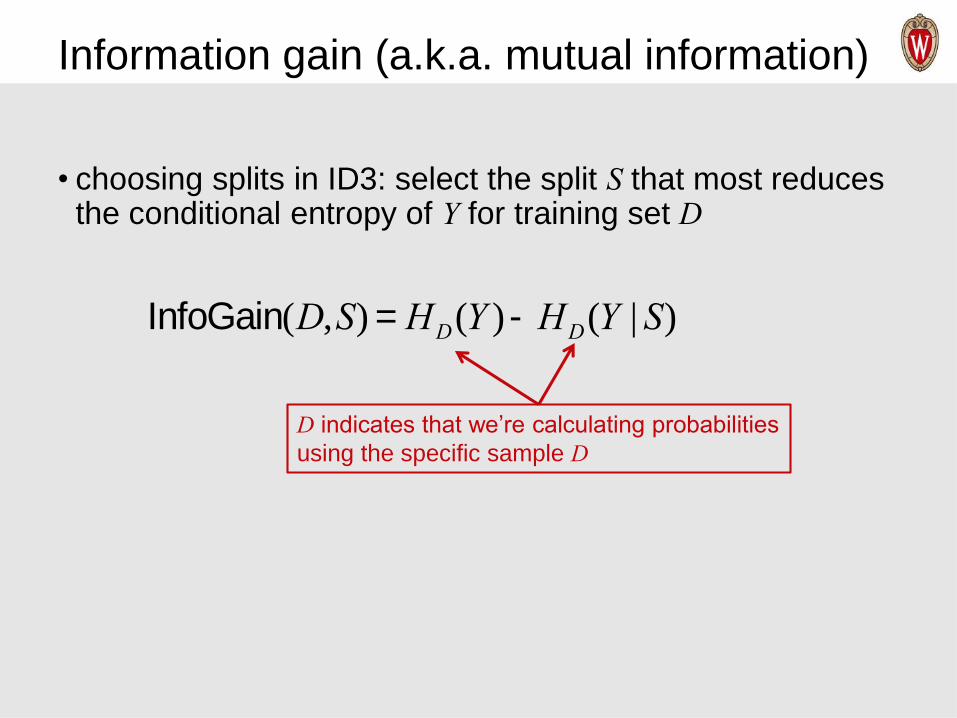
Information gain (a.k.a. mutual information)

• choosing splits in ID3: select the split S that most reduces the conditional entropy of Y for training set D

InfoGain(D,S) = HD(Y )-HD(Y | S)

D indicates that we’re calculating probabilities

using the specific sample D

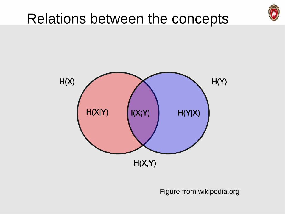
Relations between the concepts

Figure from wikipedia.org

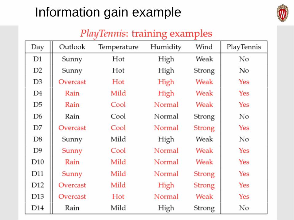
Information gain example

Information gain example

Humidity

high normal

D: [3+, 4-]

D: [9+, 5-]

D: [6+, 1-]

• What’s the information gain of splitting on Humidity?

940.014

5log

14

5

14

9log

14

9)( 22 =

−

−=YHD

592.0

7

1log

7

1

7

6log

7

6)normal|( 22

=

−

−=YHD

985.0

7

4log

7

4

7

3log

7

3)high|( 22

=

−

−=YHD

151.0

)592.0(14

7)985.0(

14

7940.0

)Humidity|()()Humidity,(InfoGain

=

+−=

−= YHYHD DD

Information gain example

Humidity

high normal

D: [3+, 4-]

D: [9+, 5-]

D: [6+, 1-]

• Is it better to split on Humidity or Wind?

HD(Y | weak) = 0.811

Wind

weak strong

D: [6+, 2-]

D: [9+, 5-]

D: [3+, 3-]

HD(Y |strong) =1.0

✔

151.0

)592.0(14

7)985.0(

14

7940.0)Humidity,(InfoGain

=

+−=D

048.0

)0.1(14

6)811.0(

14

8940.0)Wind,(InfoGain

=

+−=D

One limitation of information gain

• information gain is biased towards tests with many outcomes

• e.g. consider a feature that uniquely identifies each training instance

• splitting on this feature would result in many branches, each of which is “pure” (has instances of only one class)

• maximal information gain!

Gain ratio

• to address this limitation, C4.5 uses a splitting criterion called gain ratio

• gain ratio normalizes the information gain by the entropy of the split being considered

GainRatio(D,S) =InfoGain(D,S)

HD(S)=HD(Y )-HD(Y | S)

HD(S)

THANK YOUSome of the slides in these lectures have been adapted/borrowed

from materials developed by Mark Craven, David Page, Jude Shavlik, Tom Mitchell, Nina Balcan, Elad Hazan, Tom Dietterich,

and Pedro Domingos.