decision trees: a comparison of various algorithms for ...cs.jhu.edu/~vmohan3/document/ai_dt.pdf ·...
TRANSCRIPT
Decision Trees:A comparison of various algorithms for
building Decision Trees
Vaibhav Mohan
April 18, 2013
Abstract
Decision Trees are a decision support tool that contains tree likegraph of decisions and the possible consequences. They are commonlyused in different real world scenarios ranging from operations researchto classifying a specie in a phylum given its features.
The Decision Tree is implemented using traditional ID3 algorithmas well as an evolutionary algorithm for learning decision trees in thispaper. The Traditional Algorithm for learning decision trees is imple-mented using information gain as well as using gain ratio. Each variantis also modified to combat over-fitting using pruning. The Evolution-ary Algorithm is implemented with fitness proportionate and rankbased as their selection strategy. The algorithm is also implementedto have complete replacement and elitism as replacement strategy.The two algorithms are compared based on their accuracy, precisionand recall by varying the aforementioned parameters on the datasetstaken from UCI Machine Learning repository[2]. The time taken forlearning the Decision Tree by each algorithm corresponding to eachsetting is also compared in this paper.
1 Introduction
Classification is the problem of identifying a category for the given instancewhose category is unknown. The classifier tries to classify the given unknowninstance based on the data it learns from the training set and features it sees
1

in the instance for which prediction is to be done. This problem arises invarious fields ranging from operation research to robotics to making financialdecisions. There are wide varieties of classification problems in machinelearning domain, all of which cannot be solved using one technique [13].Therefore, for proving that the results which we are getting from one kindof technique is good enough for us makes it indispensable that we comparethe results with other techniques for the given problem. Whilst doing this,we come across the various performance aspects of the algorithm i.e. whereit would fail and where it can do remarkably well in classifying the data.
One of the most popular technique for classifying data in Machine Learn-ing domain is Decision Trees. The advantage of using Decision Trees inclassifying the data is that they are simple to understand and interpret. De-cision tree have been well studied and widely used in the knowledge discoveryand decision support system. These trees approximate discrete-valued tar-get functions as trees and are widely used practical method for inductivereference[9]. Each line present in the datasets is known as the instance. Theinstance contains the label and a vector of features present in it. The Deci-sion Trees examines the feature of given instance and comes to a conclusionon what label to assign based on the values present for the various features ofthat particular instance. Each node in the decision tree is either a decisionnode or a leaf node. This classifier resembles tree data structure as eachdecision can have two outcomes, thereby making a binary decision tree thatculminates in a label corresponding to each set of given features.
Algorithms, such as ID3, often use heuristics that tends to find shortdecision trees[9, 11], however finding the shortest decision tree is a hard op-timization problem[6]. Genetic Algorithms (GAs) are inspired by the realworld process of evolution[9, 11, 7]. GAs have been used to construct shortand near-optimal decision trees. In order to utilize genetic algorithms, deci-sion trees must be represented as chromosomes on which genetic operatorssuch as mutation and crossover can be applied. Genetic Algorithms havebeen used in two ways for finding the near-optimal decision trees. One wayis that they can be used to construct decision trees in a hybrid or preprocess-ing manner[8]. The other way is to apply them directly to decision trees[10].In this paper, we implement decision trees using traditional ID3 algorithmas well as Genetic Algorithm. The comparison of performance of both thealgorithms is done in this paper.
The remainder of paper is organized as follows. Section 2 defines the de-cision trees and the various algorithms used in implementing decision trees.
2
Section 3 comprises of details of the parameters chosen pertaining to imple-mented algorithms and experimental methods used with them. It also talksabout the datasets used for performing the experiment. Section 4 presentsthe results obtained after performing the experiment. Section 5 talks aboutthe interpretation of the data which we got from the experiment. Finally,Section 6 concludes this work.
2 Learning Decision Trees
The data classification is a two step process. The first step is training theclassifier using training data set. The second step involves predicting thelabels for the unknown datasets (or testing datasets). The decision tree is aflow chart like tree structure where each node denotes a test on an attributeand each branch denotes an outcome of the test. The leaf nodes present inthe decision trees represents classes or class distributions. This comes underthe training step. Now in order to classify an unknown instance, the attributevalues of instance are tested against decision tree and a path is traced fromroot to leaf node which holds the class prediction for that sample. This comesunder the prediction step. The decision trees can easily be converted intoclassification rules.
Decision tree falls under supervised learning techniques as we have knownlabels in the training data set in order to train the classifier. The various al-gorithms that are implemented in this paper are discussed in the subsectionsgiven below.
2.1 Traditional Methods
The traditional algorithm for building decision trees is a greedy algorithmwhich constructs decision tree in top down recursive manner. A typicalalgorithm for building decision trees is given in figure 1.
The algorithm begins with the original set X as the root node. it iteratesthrough each unused attribute of the set X and calculates the informationgain (IG). The information gain is calculated by deducting conditional en-tropy of the given attribute with the total entropy. The formulas needed tocalculate information gain along with the formula for calculating informationgain is given in the subsection given below.
The algorithm then chooses to split on the feature that has the highest
3

Figure 1: A recursive algorithm for building decision tree
information gain. The Set X is then split by the feature obtained in theprevious step to produce the subset of data depending on the value of feature.The decision tree is then built recursively until every element in the subsetbelongs to the same class, in which case, a terminal node is added to thedecision tree with a class label same as the class all its elements belong to.
Entropy and Information Gain
The information gain from the attribute test on the set of instances X is theexpected reduction in entropy. The algorithm computes the information gainof each feature and then chooses the feature with highest information gainfor splitting. The formulas needed to calculate information gain along withformula for calculating information gain is given below.
The total entropy is given by the formula:
H(X) = −n∑
i=1
p(xi) log(p(xi)), (1)
The conditional entropy is given by the formula:
H(Y |X) = −m∑i=1
n∑j=1
p(yi, xj) log(p(yi, xj)
p(xj)), (2)
and finally, the information gain (IG) is given by the formula:
IG(Y |X) = H(Y )−H(Y |X), (3)
4
The information gain is equal to total entropy for an attribute we have aunique class label for each of the given attribute values.
Information gain is a good measure for deciding the relevance of attributein general. However if we have an attribute that can take large numberof distinct values, then splitting feature based on the information gain isnot prudent. For example, consider an attribute that contains the instancenumber of each instance. Now if we use information gain heuristics, thisattribute will give the highest information gain value which would depictthat we can classify the samples perfectly. This would make the classifier toover fit the training data. Now when we see an unknown instance with valueof instance number that is not present in the training set, the classifier wouldfail to predict the label for it. In order to overcome this problem, we use anew heuristics that uses gain ratio for deciding which feature to split on.
Gain Ratio
The gain ratio biases the decision tree against considering attributes withhigher number of distinct values thereby solving the drawback of the infor-mation gain. Using gain ratio heuristics for choosing best feature to splitupon avoids over-fitting of training data. The gain ratio of an attribute iscalculated by dividing its information gain with its information value. Theformula for calculating information value is given below:
IV (Y |X) = −n∑
j=1
p(y, xj) log(p(y, xj)), (4)
The gain ratio (GR) is then given by:
GR(Y |X) =IG(Y |X)
IV (Y |X), (5)
Therefore we use gain ratio instead of information gain when searching forbest feature to split upon, avoiding the problem posed by using informationgain heuristics.
Pruning
In case of traditional algorithms for learning decision trees, when decisiontrees are built, many of the branches may reflect noise or outliers in the
5
training data. In order to combat this over-fitting, we attempt to identifyand remove such branches with the goal of improving classification accuracyon the unseen data. This is called tree pruning.
After the decision tree is made using the aforementioned algorithm, wethen traverse on each node of the tree and perform a statistical significancetest. We initially assume that there is no underlying pattern. Then actualdata is used for calculating the extent of deviation from a perfect absenceof pattern. Significant pattern is present in the data if degree of deviationis statistically unlikely. We then calculate the probability, that under nullhypothesis, a sample of size v = n + p would exhibit the observed deviationfrom the expected distribution of positive and negative examples[12]. Thedeviation is measured by comparing actual number of positive and negativeexamples in each subset, pk and nk, with the expected number of positivesand negatives, p̂k and n̂k:
The p̂k is given by -
p̂k = p× p̂k + n̂k
p + n, n̂k = n× p̂k + n̂k
p + n, (6)
The total deviation is then given by:
∆ =d∑
k=1
(pk − p̂k)2
p̂k+
(nk − n̂k)2
n̂k
, (7)
We then examine the value of ∆ to see if it confirms or rejects the null hy-pothesis. With this pruning, the over-fitting of training data can be avoidedthereby increasing the accuracy of predictions.
2.2 Genetic Algorithms
Genetic Algorithms (GAs) are adaptive heuristics search algorithm based onthe evolutionary ideas of natural selection ad genetics. They are a rapidlygrowing area of artificial intelligence and are inspired by Darwin’s theoryabout the evolution - survival of the fittest. GAs represent an intelligentexploitation of a random search used to solve optimization problems. Thoughthey are randomized, they exploit historical information to direct the searchinto the region of better performance within the search space. The ideabehind using GAs to solve the search problem in large state-space is that
6
they are good at navigating the state-space and find near-optimal solutionwhich could not have been found otherwise.
We generally start with a population of candidate solution, also calledindividuals. These individuals are evolved towards the better solution ex-ploring the state-space of the given problem. Each individual is representedusing genome encoding. The fitness function is defined such that it takes anindividual as its input and gives its fitness value. Therefore the key issuesto think about while programming a GA is its encoding and fitness function.The fitness function should be chosen wisely so that it can award fitnessscore to the individuals even when all the individuals perform badly. Thisneeds to be done because performance of all the individuals is poor at thebeginning of the search and even then the fitness function needs to drivethe search towards the part of state-space that contains better solution. Ameticulous decision about choosing the population size also needs to be done.We should not choose very small population size as it would be insufficient tocover the state-space for finding the solution. Increasing the population sizealso increases the search time of GA. We have to hand tune this parameterby running the algorithm on various population size so as to determine whatshould be the good value of population size for our problem.
Once the initial population is chosen, we then use selection schemes forselecting the individuals that are fittest among them. There are varioustechniques such as fitness proportionate and rank based strategy for selectingthe fittest individuals. Once this is done, genetic operators such as mutationand crossover is applied on them to generate the new generation and fitnessof new individuals is calculated. It is important that genetic operators aredefined in such a way so that once they give an individual after mutation orcrossover, the fitness function would still be able to calculate their fitness.Otherwise the search could not be continued. After new individuals aregenerated, we use some replacement strategy such as complete replacementor elitism so as to choose the initial population for the next iteration. Thesesteps are performed till the fitness of the population converges i.e. fitnessof two subsequent generation does not change, or the specified number ofgenerations have reached.
It is also possible that the best performing individual would be lost ifwe are completely replacing the old individuals with new ones. In order toovercome this, the algorithm remembers the best individual seen so far.
7
Genetic Algorithms for Decision Trees
From the discussion above, it is clear that we need an encoding, initial popu-lation size, fitness function, genetic operators such as mutation and crossover,selection strategy and a replacement strategy in order to solve a problem us-ing GAs. The following subsections discusses about how encoding is done,what are the selection/replacement strategies used, how genetic operatorsare implemented and how the fitness function is chosen in order to generatedecision trees using GAs.
1. Encoding: A tree based encoding scheme is used in this implementationfor encoding the population. The idea behind using tree based encodingscheme is that trees can directly be encoded and manipulated. The treeconsists of a root node which has set of child nodes. These nodes canthen either have a leaf node or a decision node. The decision nodeshave decision variables associated with them while leaf nodes contains theclass label. The tree contains child nodes corresponding to each possibleoutcome. This is a variable length encoding as the length of encoding isdependent on depth/branching factor of the tree.
2. Crossover: The crossover in this encoding scheme is straightforward. Wetraverse the trees and randomly choose a node for each and swap themto get two different trees. Swapping the two sub-trees allows for largechange in behavior preserving good behavior generated by a sub-tree.
3. Mutation: Mutation is done by randomly choosing a node in the tree andturning it into leaf node. Mutation is also done by traversing tree untila leaf node is reached and then turning that leaf node into a randomlychosen decision node. The idea behind this is that we just need a validsolution and not necessarily a good solution after this operation. Forexample even if we use same attribute as decision criteria twice in a givenpath through the tree, it is still a valid solution.
4. Selection Strategy: Selection strategy is needed in order to choose thefittest individuals from the population that are fit for crossover and mu-tation. We have implemented two types of selection strategy viz. fitnessproportionate and rank based.
In case of fitness proportionate selection strategy, the fitness is assignedto all the individuals using fitness function which is used for associating
8
a probability of selection with each individual. If fi is the fitness ofindividual i in the population, then the probability of it being selected isgiven by:
pi =fi∑Nj=1 fj
,where N is the number of individuals in the population.
(8)
The rank order based selection strategy assigns rank to each individualdepending on their fitness. The fittest individuals are then selected withprobability p for mutation and probability 1−p for crossover where p mustbe less than 0.2. This is because in general we choose lesser individualsfor mutation than crossover.
5. Replacement Strategy: Replacement strategy is needed for choosinghow many individuals do we need to keep for next generation. We haveimplemented two types of selection strategy viz. complete replacementand elitism. In case of complete replacement replacement strategy, wereplace the entire population again with new randomly generated individ-uals while we keep an amount of individuals for using as next generationpopulation in case of elitism replacement strategy.
6. Fitness Function: The fitness function is used by GAs to calculatethe fitness of an individual. We have implemented three kind of fitnessfunction based on accuracy, precision and recall given by the individualdecision tree on the training data. The fitness function takes an individualas its inputs and gives its fitness as output. In this case our input is adecision tree. We then use this decision tree for predicting labels ontraining data and calculate its accuracy/precision/recall depending onwhat fitness function is used and then return the fitness of the individual.We finally chose fitness function based on the accuracy. This is becausewe wanted to maximize the accuracy of prediction in case of each datasets.
9

3 Algorithms and Experimental Methods
Traditional Algorithm
There were various parameters to choose in case of traditional algorithmlike whether to use gain ratio or information gain for splitting the features,whether we should make algorithm to do pruning or not etc. We chose to usegain ratio as it is a better heuristics than information gain. The results ofcomparison of algorithm using gain ratio and using information gain is givenin the next section. The algorithm also have parameter for using pruning inorder to combat over-fitting. The experimentation was done using algorithmwith pruning and without pruning. The accuracy, precision and recall wascalculated on training set as well as testing set and was compared with theother algorithm. A comparison of time taken in training the algorithms onvarious datasets is also done.
Genetic Algorithm
There were various tunable parameters such as number of generations, pop-ulation size, whether to use rank based or fitness proportionate strategy andwhether to use complete replacement or elitism as the replacement strategy.The experimentation was done by varying population size and found that apopulation size of 1000 is a good selection for this problem. Also the numberof generations was varied from 100 to 10000 and found that almost all thedata sets converge after 800 generations. Hence the number of generationswas fixed to 1000 to be safe. We also experimented with the selection strat-egy and found that rank based selection strategy is good for our problem.We further experimented with replacement strategy and found that the re-sults were same for elitism and complete replacement strategy. The resultsof these experimentations are given in the next section. The accuracy, preci-sion and recall was calculated on training set as well as testing set and wascompared with the other algorithm. A comparison of time taken in trainingthe algorithms on various datasets is also done.
Data Sets
All the datasets used in performing the experiment was obtained from UCImachine learning database [2]. All the datasets were processed by parsers
10

implemented by us specific to each datasets and was converted into integerformat from string format. This was done so that we can have homogeneoustype of data. This way we decoupled the algorithm from the type of datapresent in the file i.e. no matter what kind of data we have in the file, thealgorithm always gets data in the integer format. Therefore if we want to useany other dataset with this algorithm, all we need to do is write a parser thatconverts the data into integer format and we could still use this algorithm inpredicting labels for that dataset. The details pertaining to each datasets,their properties, and how they are processed is described in the sections givenbelow.
1. Congressional Voting Data: This dataset was obtained from UCI ma-chine learning database[1]. This dataset contains two class labels namelyrepublican and democrat. There are 17 binary attributes in the datasets.The first attribute represents the class label and the rest of attributesdefine the feature of the instance that is associated with it. Each line inthis data file contains an example comprising of 17 attributes. All theattributes were of yes/no type. The given data file had 435 instances init. We randomly chose 70% of examples for training the classifier andremaining 30% for testing the classifier.
The class label democrat was encoded to 0 and republican was encodedto 1. The attribute value y was encoded to 1 and value n was encodedto 0. We also had missing data in some attributes which was representedby ’?’ in the original data file. We treated this value as third value whichmeant abstain i.e. no opinion was recorded. This value was encoded to2.
2. Monk’s Problems Data: This dataset was obtained from UCI machinelearning database[3]. The Monk’s problem dataset had 6 files 3 each fortesting and training the classifier. This dataset contains two class labelsnamely 0 and 1. There are 8 attributes in the datasets. The first attributerepresents the class label and the rest of attributes define the feature ofthe instance that is associated with it. Each line in this data file containsan example comprising of 8 attributes. Some of the attributes given inthis data file had 4 distinct values however none of the attributes tookmore than 4 distinct values. Each of the given data file had 432 instancesin it.
11
The class label 0 was encoded to 0 and 1 was encoded to 1. The attributevalue 1, 2, 3, 4 were represented as 1, 2, 3, 4 in integer format after parsing.These files did not have any missing data.
3. Mushroom Data: This dataset was obtained from UCI machine learn-ing database[4]. This dataset contains the information about the physicalproperties of the mushroom specimen. This dataset contains two classlabels namely e which stands for edible mushroom and p which stands forpoisonous mushroom i.e. they are unfit for consumption. There are 23attributes in the datasets. The first attribute represents the class labeland the rest of attributes define the feature of the instance that is asso-ciated with it. Each line in this data file contains an example comprisingof 23 attributes. Some of the attributes given in this data file had manydistinct values in them. The given data file had 8124 instances in it. Werandomly chose 70% of examples for training the classifier and remaining30% for testing the classifier.
The class label e was encoded to 1 and p was encoded to 0. The attributevalue varied from a . . . z so we encoded them as a = 1, b = 2, c = 3 . . . .We also had missing data in some attributes which was represented by’?’ in the original data file. There was only one attribute that containedmissing values in it so that attribute was dropped.
4. Splice Junction Data: This dataset was obtained from UCI machinelearning database[5]. This dataset contains data from a molecular biologyproblem. The goal is to recognize boundaries between introns and exons.This dataset had 2 files 1 each for testing and training the classifier. Thisdataset contains multiple class labels namely ie, which represents intron-exon boundary, ei, which represents exon-intron boundary, and n whichmeans neither boundary. There are 62 attributes in the datasets. Thefirst attribute represents the class label, the second attribute gives theinstance name and the remaining 60 fields are the sequence, starting atposition -30 and ending at position +30. Each of these fields is almostalways filled by one of a, g, t, c. Each line in this data file contains anexample comprising of 62 attributes. All the attributes in this file weremulti valued attributes.The given data file had 3190 instances in it. Werandomly chose 70% of examples for training the classifier and remaining30% for testing the classifier.
The class label ie was encoded to 0, ei was encoded to 1 and n was
12

Dataset Train/Test Heuristic use pruning? Accuracy Precision Recall
Congressional Train IG no 1.0 1.0 1.0Congressional Test IG no 0.9389 0.94 0.9038Congressional Train GR no 1.0 1.0 1.0Congressional Test GR no 0.9389 0.94 0.9038Congressional Train IG yes 0.9145 1.0 0.9719Congressional Test IG yes 0.9549 1.0 0.9342Congressional Train GR yes 0.9145 1.0 0.9719Congressional Test GR yes 0.9549 1.0 0.9342
Table 1: Performance results of traditional algorithm with different variationsusing congressional datasets.
encoded to 2. The attribute value a, c, g, t were represented as 0, 1, 2, 3respectively after parsing. The other characters in attributes were alsoencoded to 3. These files did not have any missing data.
4 Results
Table 1 through 4 shows the results of traditional algorithm on congressionaldataset, monks datasets, mushroom dataset and splice junction dataset re-spectively. The value of parameters were varied as shown in the table andcorresponding accuracy, precision and recall was recorded.
Table 5 through 8 shows the results of genetic algorithm on congressional,monks problem, mushroom and splice junction datasets respectively. Thevalue of parameters were varied as shown in the table and correspondingaccuracy, precision and recall was recorded. The value of population size wasset to 1000 and number of generations was fixed to 1000. These parameterswere chosen after experimenting with their different values and recording theaccuracy. Here FP means fitness proportionate, RB means rank based, CRmeans complete replacement and El means elitism.
Table 9 shows the time taken by algorithms to train on each datasets.The time was recorded by choosing gain ratio as heuristics and using treepruning in case of traditional algorithm and using fitness proportionate selec-tion strategy and elitism as replacement strategy in case of genetic algorithm.The population size was fixed to 1000 and number of generations was also
13

Dataset Train/Test Heuristic use pruning? Accuracy Precision Recall
Monks 1 Train IG no 0.9355 0.9091 0.9677Monks 1 Test IG no 0.8194 0.776 0.8982Monks 1 Train GR no 0.9355 0.8971 0.9838Monks 1 Test GR no 0.8194 0.7593 0.9351Monks 1 Train IG yes 0.8226 0.8704 0.7581Monks 1 Test IG yes 0.7431 0.7664 0.6991Monks 1 Train GR yes 0.9355 0.9091 0.9677Monks 1 Test GR yes 0.8333 0.7951 0.8981
Monks 2 Train IG no 0.9408 0.9355 0.9063Monks 2 Test IG no 0.838 0.7195 0.838Monks 2 Train GR no 1.0 1.0 1.0Monks 2 Test GR no 0.8935 0.7857 0.9296Monks 2 Train IG yes 0.9145 0.9291 0.8951Monks 2 Test IG yes 0.8549 0.7374 0.8342Monks 2 Train GR yes 1.0 1.0 1.0Monks 2 Test GR yes 0.8935 0.7857 0.9296
Monks 3 Train IG no 0.8279 0.8421 0.8Monks 3 Test IG no 0.6389 0.6915 0.5702Monks 3 Train GR no 0.8525 0.85 0.85Monks 3 Test GR no 0.6296 0.67 0.5878Monks 3 Train IG yes 0.8279 0.8421 0.8Monks 3 Test IG yes 0.6389 0.6915 0.5702Monks 3 Train GR yes 0.8525 0.8621 0.8333Monks 3 Test GR yes 0.6389 0.6915 0.5702
Table 2: Performance results of traditional algorithm with different variationsusing Monk’s Problem datasets.
14
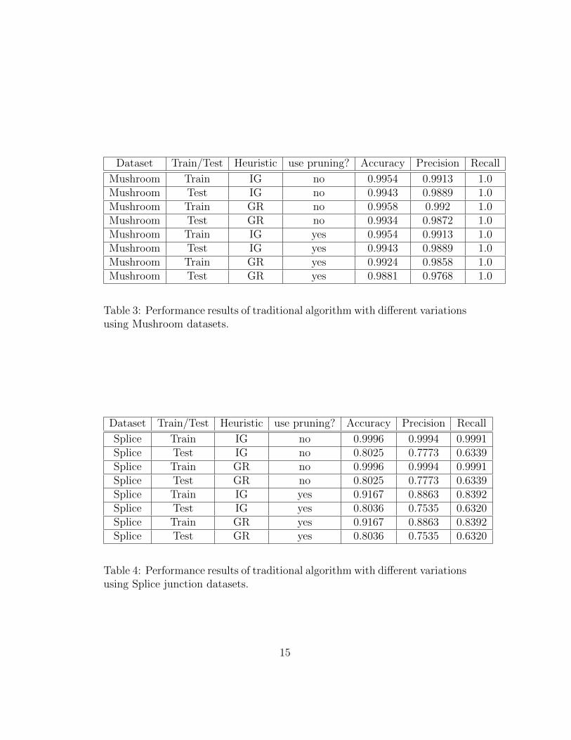
Dataset Train/Test Heuristic use pruning? Accuracy Precision Recall
Mushroom Train IG no 0.9954 0.9913 1.0Mushroom Test IG no 0.9943 0.9889 1.0Mushroom Train GR no 0.9958 0.992 1.0Mushroom Test GR no 0.9934 0.9872 1.0Mushroom Train IG yes 0.9954 0.9913 1.0Mushroom Test IG yes 0.9943 0.9889 1.0Mushroom Train GR yes 0.9924 0.9858 1.0Mushroom Test GR yes 0.9881 0.9768 1.0
Table 3: Performance results of traditional algorithm with different variationsusing Mushroom datasets.
Dataset Train/Test Heuristic use pruning? Accuracy Precision Recall
Splice Train IG no 0.9996 0.9994 0.9991Splice Test IG no 0.8025 0.7773 0.6339Splice Train GR no 0.9996 0.9994 0.9991Splice Test GR no 0.8025 0.7773 0.6339Splice Train IG yes 0.9167 0.8863 0.8392Splice Test IG yes 0.8036 0.7535 0.6320Splice Train GR yes 0.9167 0.8863 0.8392Splice Test GR yes 0.8036 0.7535 0.6320
Table 4: Performance results of traditional algorithm with different variationsusing Splice junction datasets.
15
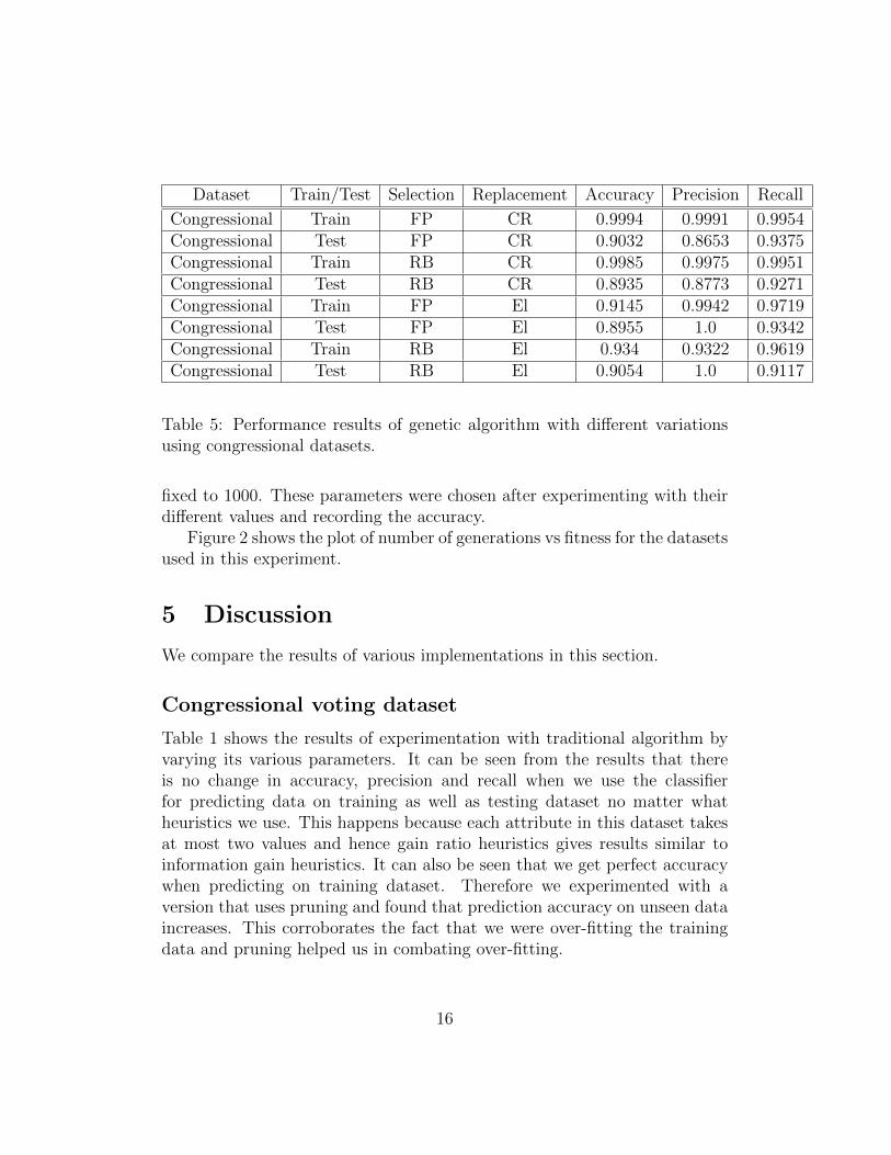
Dataset Train/Test Selection Replacement Accuracy Precision Recall
Congressional Train FP CR 0.9994 0.9991 0.9954Congressional Test FP CR 0.9032 0.8653 0.9375Congressional Train RB CR 0.9985 0.9975 0.9951Congressional Test RB CR 0.8935 0.8773 0.9271Congressional Train FP El 0.9145 0.9942 0.9719Congressional Test FP El 0.8955 1.0 0.9342Congressional Train RB El 0.934 0.9322 0.9619Congressional Test RB El 0.9054 1.0 0.9117
Table 5: Performance results of genetic algorithm with different variationsusing congressional datasets.
fixed to 1000. These parameters were chosen after experimenting with theirdifferent values and recording the accuracy.
Figure 2 shows the plot of number of generations vs fitness for the datasetsused in this experiment.
5 Discussion
We compare the results of various implementations in this section.
Congressional voting dataset
Table 1 shows the results of experimentation with traditional algorithm byvarying its various parameters. It can be seen from the results that thereis no change in accuracy, precision and recall when we use the classifierfor predicting data on training as well as testing dataset no matter whatheuristics we use. This happens because each attribute in this dataset takesat most two values and hence gain ratio heuristics gives results similar toinformation gain heuristics. It can also be seen that we get perfect accuracywhen predicting on training dataset. Therefore we experimented with aversion that uses pruning and found that prediction accuracy on unseen dataincreases. This corroborates the fact that we were over-fitting the trainingdata and pruning helped us in combating over-fitting.
16

Dataset Train/Test Selection Replacement Accuracy Precision Recall
Monks 1 Train FP CR 0.8321 0.8491 0.8654Monks 1 Test FP CR 0.7532 0.696 0.8051Monks 1 Train RB CR 0.8309 0.8472 0.8683Monks 1 Test RB CR 0.7654 0.7152 0.7966Monks 1 Train FP El 0.8226 0.8704 0.7581Monks 1 Test FP El 0.7431 0.7664 0.6991Monks 1 Train RB El 0.8135 0.8291 0.8635Monks 1 Test RB El 0.7374 0.7092 0.8265
Monks 2 Train FP CR 0.7925 0.8086 0.7851Monks 2 Test FP CR 0.7532 0.696 0.7784Monks 2 Train RB CR 0.8321 0.8491 0.8654Monks 2 Test RB CR 0.7532 0.696 0.8051Monks 2 Train FP El 0.9408 0.9655 0.875Monks 2 Test FP El 0.83 0.7237 0.7746Monks 2 Train RB El 0.9355 0.9091 0.9677Monks 2 Test RB El 0.8132 0.7856 0.8783
Monks 3 Train FP CR 0.7577 0.7532 0.7231Monks 3 Test FP CR 0.6054 0.6374 0.5306Monks 3 Train RB CR 0.7754 0.8032 0.7941Monks 3 Test RB CR 0.6352 0.6723 0.5459Monks 3 Train FP El 0.8177 0.8232 0.77Monks 3 Test FP El 0.63 0.677 0.5502Monks 3 Train RB El 0.8171 0.8229 0.7673Monks 3 Test RB El 0.6365 0.6712 0.5512
Table 6: Performance results of genetic algorithm with different variationsusing Monk’s Problem datasets.
17

Dataset Train/Test Selection Replacement Accuracy Precision Recall
Mushroom Train FP CR 0.9991 1.0 1.0Mushroom Test FP CR 0.9933 1.0 1.0Mushroom Train RB CR 0.9925 0.9968 0.9954Mushroom Test RB CR 0.9914 0.9964 0.9995Mushroom Train FP El 0.9953 0.99 0.9975Mushroom Test FP El 0.9946 0.9895 0.9894Mushroom Train RB El 0.9955 0.9991 0.9977Mushroom Test RB El 0.9933 0.9951 0.9981
Table 7: Performance results of genetic algorithm with different variationsusing Mushroom datasets.
Dataset Train/Test Selection Replacement Accuracy Precision Recall
Splice Train FP CR 0.9619 0.9457 0.9312Splice Test FP CR 0.7951 0.805 0.6343Splice Train RB CR 0.9551 0.949 0.9531Splice Test RB CR 0.8031 0.7743 0.6742Splice Train FP El 0.9755 0.9597 0.9587Splice Test FP El 0.813 0.793 0.6585Splice Train RB El 0.9639 0.9493 0.9482Splice Test RB El 0.8015 0.8132 0.6365
Table 8: Performance results of genetic algorithm with different variationsusing Splice junction datasets.
Dataset Training Time (traditional) Training Time (GA)
Congressional 41 ms 226505 msMonks 1 12 ms 266819 msMonks 2 20 ms 365224 msMonks 3 15 ms 268876 ms
Mushroom 246 ms 918150 msSplice 419 ms 1415455 ms
Table 9: Training time taken by various algorithms on all datasets.
18
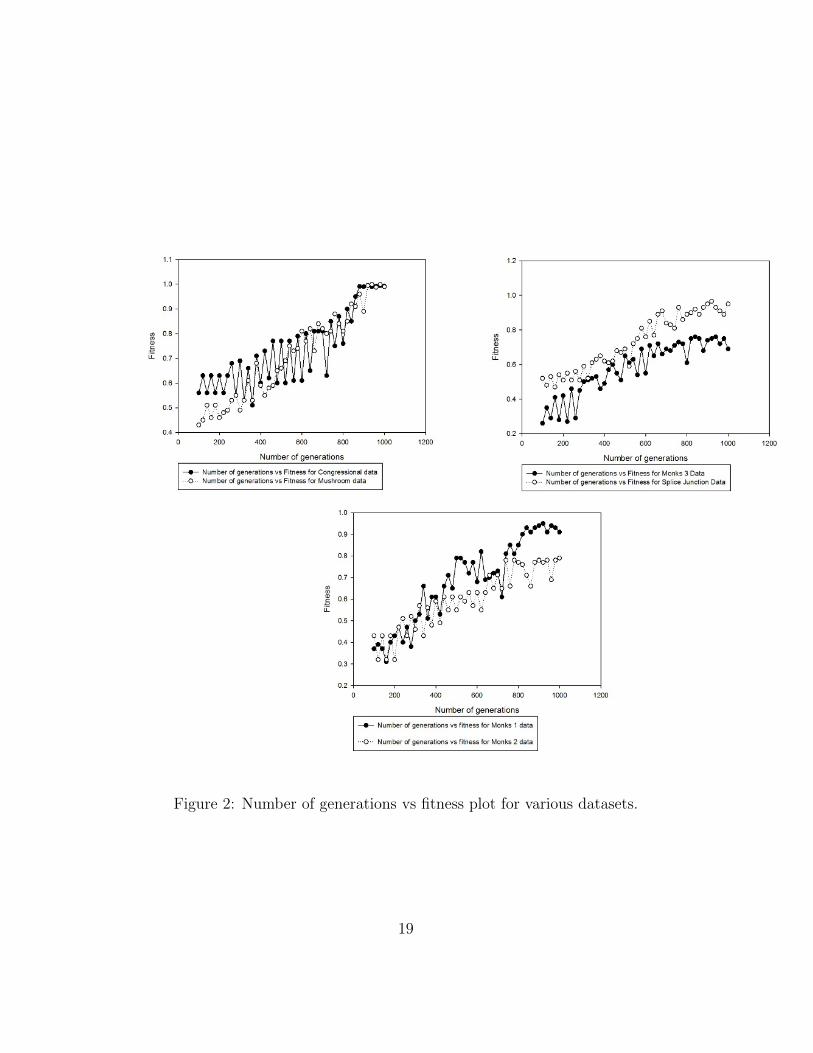
Figure 2: Number of generations vs fitness plot for various datasets.
19
Table 5 shows the results of experimentation with genetic algorithm byvarying its various parameters. It can be seen from the results that we gethighest accuracy when we use rank based selection strategy and elitism asreplacement strategy. All the other variations give almost similar results.
It can be seen from the results of Table 1 and 5 that traditional algorithmperforms better as compared to genetic algorithm in this case however thedifference in prediction accuracy is very small.
Monk’s Problem dataset
Table 2 shows the results of experimentation with traditional algorithm byvarying its various parameters. It can be seen from the results that thereis no change in accuracy, precision and recall when we use the classifierfor predicting data on training as well as testing dataset no matter whatheuristics we use. This might be happening because the attributes does nothave many distinct values in case of this dataset.We also experimented witha version that uses pruning and found that prediction accuracy on unseendata is almost similar corroborating the fact that we were not over-fitting thetraining data. It can also be seen that the classifier doesn’t do well on theMonks 3 dataset. This would be because the given dataset contains morenoise as compared to the other datasets thereby decreasing the predictionaccuracy.
Table 6 shows the results of experimentation with genetic algorithm byvarying its various parameters. It can be seen from the results that we gethighest accuracy when we use rank based selection strategy and completereplacement as replacement strategy in case of Monks 1 data. Monks 2 datagives highest accuracy when we use fitness proportionate selection schemeand elitism as replacement strategy. Monks 3 data gives highest accuracywhen we use rank based selection scheme and elitism as replacement method.All the other variations give almost similar results.
It can be seen from the results of Table 2 and 6 that traditional algorithmperforms significantly better than genetic algorithm on all the given datasetsof Monk’s problem. This could be because the state-space of Monk’s problemis very large and genetic algorithm would not be able to explore it fully.
20
Mushroom dataset
It can be seen from the table 3 that varying the parameters of traditionalalgorithm does not affect the accuracy, precision and recall in this case. Thismight be happening because the data set might not be having any noiseas well as all the attributes take almost similar number of distinct valuesthereby rendering gain ratio and pruning useless in this case.
Table 7 shows similar results as table 3 substantiating the fact that geneticalgorithm performs similar to traditional algorithm.
Splice Junction dataset
It is evident from table 4 that there is no change in accuracy, precision andrecall when we use the classifier for predicting data on training as well astesting dataset no matter what heuristics we use. This might be happeningbecause the attributes does not have many distinct values in case of thisdataset. We also experimented with a version that uses pruning and foundthat prediction accuracy on unseen data is almost similar to the version thatdoes not use pruning. This might be happening because the datasets mightnot be having much noise in it.
Table 8 shows similar results as table 4 substantiating the fact that geneticalgorithm performs similar to traditional algorithm in this case.
Training time on datasets
It can be seen from table 9 that training classifier using traditional algorithmrequires substantially lesser time than genetic algorithm. This happens be-cause genetic algorithm uses many agents to search the space which requiresa large amount of computation time and hence training the algorithm usingGA takes longer.
Fitness of individuals with respect to generation
Figure 2 shows the number of generations vs fitness plot for various datasets. The population size was fixed to 1000 for plotting these graphs. It can beseen from the graphs that all the classifiers had bad fitness when algorithmstarted its execution and eventually their fitness kept growing. The algorithmconverged in almost all the cases near 800th generation. After that there
21
was very less fluctuation of fitness in all the cases. Hence the parameter fornumber of generations was fixed to 1000. It might have been possible thatthe algorithm would have found even better solution. This would requiremore number of generations which would consume even more time.
6 Conclusions
It have been shown that traditional algorithm have performed well in almostall the cases as compared to the genetic algorithm. It is also seen that trainingclassifier using genetic algorithm takes longer as compared to traditionalalgorithm. However GAs are capable of solving a large variety of problemswhere traditional decision tree algorithm might fail. For example, we can getreally good accuracy in case of noisy data with genetic algorithm while thetraditional algorithm would fail to do that as it might also learn noise whiletraining on the given data.
The limitation of our approach was that we were doing completely randomsearch and then trying to move towards a favorable state. Combining ID3algorithm with GAs might help in overcoming this limitation. This approachwould have some idea about the point from where search could be startedand it might get to more optimal solution while exploring the state-space.
References
[1] D.J. Newman A. Asuncion. Uci ma-chine learning repository congressional votingdata[http://archive.ics.uci.edu/ml/datasets/congressional+voting+records],2007.
[2] D.J. Newman A. Asuncion. Uci machine learning repository[http://www.ics.uci.edu/ mlearn/mlrepository.html], 2007.
[3] D.J. Newman A. Asuncion. Uci machine learning repository monk’sproblems data[http://archive.ics.uci.edu/ml/datasets/monk
[4] D.J. Newman A. Asuncion. Uci machine learning repository mushroomdata[http://archive.ics.uci.edu/ml/datasets/mushroom], 2007.
22
[5] D.J. Newman A. Asuncion. Uci ma-chine learning repository splice junctiondata[http://archive.ics.uci.edu/ml/datasets/molecular+biology+2007.
[6] L.H. Bodlaender and H. Zantema. Finding small equivalent decisiontrees is hard. International Journal of Foundations of Computer Science,11(2):343–354, 2000.
[7] D. L. Goldberg. Genetic Algorithms in Search, Optimization, and Ma-chine Learning. Addison-Wesley, 1989.
[8] H. Vafaie K. DeJong J. Bala, J. Huang and H. Wechsler. Hybrid learn-ing using genetic algorithms and decision tress for pattern classification.Proceedings of the 14th International Joint Conference on Artificial In-telligence, Montreal, Canada, pages 719–724, 1995.
[9] T. M. Mitchell. Machine Learning. McGraw hill, 1997.
[10] A. Papagelis and D. Kalles. Ga tree: genetically evolved decision trees.Proceedings of 12th IEEE International Conference on Tools with Arti-ficial Intelligence, pages 203–206, 2000.
[11] P. E. Hart R. O. Duda and D. G. Stork. Pattern Classification, 2nd Ed.Wiley interscience, 2001.
[12] S. Russell and P. Norvig. Artificial Intelligence : A Modern Approach,3rd Ed. Prentice Hall, 2009.
[13] D. H. Wolpert and W. G. Macready. No free lunch theorems for opti-mization. Evolutionary Computation, IEEE Transactions on, 1(1):67–82, 1997.
23