NeuroImage 83 (2013) 921–936

Contents lists available at ScienceDirect

NeuroImage

j ourna l homepage: www.e lsev ie r .com/ locate /yn img

Decoding magnetoencephalographic rhythmic activity usingspectrospatial information

Jukka-Pekka Kauppi a,b,⁎, Lauri Parkkonen b,c, Riitta Hari b, Aapo Hyvärinen a,d

a Department of Computer Science and HIIT, University of Helsinki, Helsinki, Finlandb Brain Research Unit, O.V. Lounasmaa Laboratory, School of Science, Aalto University, Espoo, Finlandc Department of Biomedical Engineering and Computational Science, School of Science, Aalto University, Espoo, Finlandd Department of Mathematics and Statistics, University of Helsinki, Helsinki, Finland

⁎ Corresponding author. Department of Computer SHelsinki, Helsinki, Finland.

E-mail addresses: jukka-pekka.kauppi@helsinki.fi (J.-P. K(L. Parkkonen), riitta.hari@aalto.fi (R. Hari), aapo.hyvarinen

1053-8119/$ – see front matter © 2013 Elsevier Inc. All rihttp://dx.doi.org/10.1016/j.neuroimage.2013.07.026

a b s t r a c t

a r t i c l e i n f o

Article history:Accepted 5 July 2013Available online 18 July 2013

Keywords:DecodingMagnetoencephalographyRhythmic activityTime–frequency analysisLinear discriminant analysisIndependent component analysis

We propose a new data-driven decoding method called Spectral Linear Discriminant Analysis (Spectral LDA) forthe analysis ofmagnetoencephalography (MEG). Themethod allows investigation of changes in rhythmic neuralactivity as a result of different stimuli and tasks. The introduced classification model only assumes that each“brain state” can be characterized as a combination of neural sources, each of which shows rhythmic activity atone or several frequency bands. Furthermore, the model allows the oscillation frequencies to be different foreach such state. We present decoding results from 9 subjects in a four-category classification problem definedby an experiment involving randomly alternating epochs of auditory, visual and tactile stimuli interspersedwith rest periods. The performance of Spectral LDAwas very competitive comparedwith four alternative classifiersbased ondifferent assumptions concerning the organization of rhythmic brain activity. In addition, the spectral andspatial patterns extracted automatically on the basis of trained classifiers showed that Spectral LDA offers a noveland interesting way of analyzing spectrospatial oscillatory neural activity across the brain. All the presentedclassification methods and visualization tools are freely available as a Matlab toolbox.

© 2013 Elsevier Inc. All rights reserved.

Introduction

Unveiling neuronal information processing in the humanbrain duringreal-world experiences is a central challenge in cognitive neuroscience(Spiers and Maguire, 2007). Conventionally, functional neuroimagingstudies have been applied using relatively simple patterns of sensorystimuli, and little is known about how the human brain operateswith real-world sensory input.More recently, the neuroimaging commu-nity has started to introduce more naturalistic experimental conditions(Hasson et al., 2004, 2008; Hejnar et al., 2007; Kauppi et al., 2010;Lahnakoski et al., 2012; Wolf et al., 2010), and even “two-person neuro-science” has been advocated to record brain activity simultaneouslyfrom two interacting subjects (for a review, see Hari and Kujala (2009)).

Due to the diversity of the stimuli and/or the complexity of the exper-imental settings mimicking real-world conditions, it may be necessaryto use data-driven analysis methods that allow investigation of brainfunction without stringent assumptions about the underlying brainmechanisms (Spiers and Maguire, 2007). One of the most promisingdata-driven approaches to analyze complex brain-imaging signals is“decoding”, which gathers information frommultiple brain imaging sig-

cience and HIIT, University of

auppi), lauri.parkkonen@aalto.fi@helsinki.fi (A. Hyvärinen).

1 Hence, the terms “decoder” or “decoding model” may refer either to a classifier or aregression model.

ghts reserved.

nals to deduce the task, stimuli or brain state during the measurement.Most commonly, multivariate classifiers are used to discriminatebetween categories (Blankertz et al., 2011; Cox and Savoy, 2003;Kamitani and Tong, 2005; Mitchell et al., 2004; Murphy et al., 2011)but decoding can also be performed using regression in more complexexperimental settings (Carroll et al., 2009; Kauppi et al., 2011).1

Brain-function decoding can advance our knowledge in differentways. For instance, above-chance classification performance for an in-dependent test data set implies the presence of mutual information be-tween themeasured signals and the categories of interest (Kriegeskorte,2011). Thus, decoding can be used to test for the presence of specificstimulus information in the region of interest or across the wholebrain. Additionally, investigating how the trained models are fitted tothe brain-imaging signals tells where and how information is processedand represented in the brain. For instance, the coefficients of the linearclassifier may provide hints of brain regions involved in the processingand discrimination of the stimuli (see e.g. Rasmussen et al. (2012)).It is also possible to construct several decoders based on different neuro-scientific hypotheses and compare their performances. A priori knowledgecan be incorporated to the decoder design for instance in the form ofneuroscientifically inspired feature transformations (see e.g. Richiardi

922 J.-P. Kauppi et al. / NeuroImage 83 (2013) 921–936

et al. (2011)) or it can be embeddedmore directly to themodel design (seee.g. Tomioka and Müller (2010)).

So far, most decoding studies in neuroscience have used functionalmagnetic resonance imaging (fMRI) signals to demonstrate spatial pat-terns related to different tasks or stimulus categories (Haynes and Rees,2006; Tong and Pratte, 2012). However, the poor temporal resolution offMRI makes it inherently unsuitable for investigating the fine spectraland temporal signatures of information encoding. Instead, the brain'soscillatory electrical activity has been suggested to have a centralrole in information processing, and distinct oscillation frequencies andamplitudes even in the same neuronal structure reflect different brainstates (Singer, 1993). Large neuronal populations can generate synchro-nized oscillatory electrical activity that can be enhanced or suppressedby tasks and stimuli, and the dynamics of brain oscillations associ-ated with distinct brain states forms complex spatiotemporal patterns(Buzsáki and Draguhn, 2004). Thus, to understand brain functionduring real-world experiences, it seems necessary to interpret at thesame time the spatial, temporal and spectral signatures of brain activity.

Magnetoencephalography (MEG) has a millisecond-range temporalresolution and has therefore potential to reveal detailed spectral andtemporal characteristics of distinct brain states induced by specifictasks or stimuli. Nevertheless, decoding on the basis of MEG signalscannot be expected to be an easy task. Several factors, includingthe low signal-to-noise ratio (SNR) of single-epoch measurementsand the high dimensionality of whole-scalp recordings, make thedecoding based on MEG signals very challenging. In addition, MEGsignals do not vary only between different individuals under the sameexperimental condition, but to some extent also within the same sub-ject between repeated identical sessions, which makes it complicatedto construct a highly generalizable classifier across sessions and/orindividuals. However, training of the multivariate model based onsingle-epochs provides inevitable advantages over a univariate analysisbased on averaged epochs. For instance, a decoding approach allowsfinding combinations of the most discriminative features (or sensors)among a high number of initial features, and provides a principledway of assessing the goodness of the discrimination in terms of the es-timated generalization accuracy.

Previously, Besserve et al. (2007) used band-limited power andphase synchrony features to classify betweenMEGdata recorded duringa visuomotor task and rest condition. Rieger et al. (2008) used temporalfeatures and wavelet coefficients to predict the recognition of naturalscenes from single-trial MEG recordings. Ramkumar et al. (2013) usedboth time-resolved and time-insensitive classifiers to decode fromsingle-epoch MEG low-level visual features in the early visual cor-tex. Zhdanov et al. (2007) used temporal features together with theregularized linear discriminant analysis (regularized LDA) to classi-fy between two different visual categories (faces and houses) onthe basis of MEG signals. In the “Mind Reading from MEG” chal-lenge organized in conjunction with the International Conferenceon Artificial Neural Networks (ICANN 2011), the task was to designa classifier to distinguish between different movie categories on thebasis of 204-channel gradiometer MEG data (Klami et al., 2011). Thedata were recorded from a single subject who was shown five differentmovie clips. Thewinners of the competition extracted statistical featuresfrom time-domain signals and applied sparse logistic regression forclassification (Huttunen et al., 2012).

Decoding has also been applied to electroencephalographic (EEG)signals. For instance,Murphy et al. (2011) and Simanova et al. (2010) suc-cessfully decoded abstract semantic categories from EEG data. Moreover,Chan et al. (2011) used temporal features in the classificationof MEG and EEG data recorded simultaneously while the subjectsperformed visual and auditory language tasks.

Classification on the basis ofMEG signals has also been studied in thecontext of brain–computer interfaces (BCIs), communicationpathwaysbe-tween brains and external devices (Bahramisharif et al., 2010; Mellingeret al., 2007; Santana et al., 2012; van Gerven and Jensen, 2009). A

successful BCI has to distinguish between brain signatures of the users in-tentions, and both temporal and spectral features have been applied, oftenselected based on specific a priori knowledge of the brain function. For in-stance, preparation tomoveahand is associatedwith abrief suppressionofthe Rolandicmu rhythm that comprises 7–13 Hz and 15–25 Hz frequencybands. The power estimates characterizing these specific oscillationsoriginating from the sensorimotor cortex have been successfully appliedto decode motor-imagery tasks, where an individual mentally simulatesdifferent motor actions, such as hand movements (Pfurtscheller andNeuper, 2001). Even though most of the BCI literature has concentratedon classification on the basis of EEG, many technical advances in thisfield may also benefit MEG-based decoding; see for instance Lemm et al.(2011), Tomioka and Müller (2010), Dyrholm et al. (2007a), Liu et al.(2010), Blankertz et al. (2011), Mellinger et al. (2007), Suk and Lee(2013). On the other hand, the existing best BCI methods are not directlyapplicable to our setting because the goals of the analyses and experimen-tal conditions are different. In BCI, the only goal is maximum classificationaccuracy, while in brain-function decoding, it is important to obtain adecoder with a meaningful interpretation to advance understanding ofbrain function. Consequently, many recent neuroimaging studies haveconcentrated on the interpretation of the decoding models (Carroll et al.,2009; de Brecht and Yamagishi, 2012; De Martino et al., 2008; Grosenicket al., 2013; Rasmussen et al., 2012; Ryali et al., 2012; van Gerven et al.,2009; van Gerven et al., 2010; Yamashita et al., 2008).

Here, we constructed a brain decoding system for MEG with theexplicit goal of providing an easily interpretable decoder, as well as ageneral-purpose decoding toolbox for neuroscientific research. As anexample of this approach, we analyzed MEG data from an experimentwhere the subjectswere exposed to blocks of auditory, visual and tactilestimuli interspersed with rest blocks (Malinen et al., 2007; Ramkumaret al., 2012). We aimed to decode four distinct brain states, that is, “au-ditory”, “visual”, “tactile”, and “rest”.

The stimuli were complex, comprising video clips of people andurban scenes, speech sounds and tone beeps, as well as tactile stimulito finger tips, all presented in brief blocks of varying duration withinthe same session. Because sensory stimuli are known to activate dis-crete projection areas, we considered this experiment well-suited forthe validation of our method. However, the applied complex stimuli(speech and videos) may also activate higher-order processing. For in-stance, although it is plausible that variations in oscillatory activity inthe visual cortex aremainly responsible for discriminating the visual cat-egory from the other categories, higher-order brain processes may in-volve additional neural activity in other brain regions, therebycomplicating the decoding task. On the other hand, the diversity of thestimuli makes the decoding problem also more interesting, advocatingthe use of data-driven approaches based on relativelyweak a priori infor-mation. As our goal was to build a classifier to infer brain function in anexploratory manner, we did not impose strong assumptions on spectralcontents or spatial locations of the underlying neural activity; instead,we tried to capture the most relevant spectrospatial features automati-cally from a large number (L = 204) of MEG channels across a relativelywide frequency band (5–30 Hz).

Materials and methods

Naturalistic stimulation

We analyzed MEG data (306-channel Elekta Neuromag MEGsystem (Elekta Oy, Helsinki, Finland), filtered to 0–200 Hz anddigitized at 600 Hz) from a previous experiment (Ramkumar et al.,2012). Eleven healthy adults (6 females, 5 males; mean age 30 years,range 23–41 years) were exposed to 6–33 s blocks of auditory, visualand tactile stimuli. Similar to Ramkumar et al. (2012), data of onlynine of the eleven subjects were used in the analysis; data from twosubjects were discarded due to improper delivery of auditory stimuli.

923J.-P. Kauppi et al. / NeuroImage 83 (2013) 921–936

The stimulus blocks were interleaved with 15-s rest periods(the entire session contained 24 rest periods). Two independent12-min sessions were recorded from each subject. We exclusivelyused the first session for classifier training and the second sessionfor the evaluation the performance of the classifier. Hence, thetraining and test data sets were independent from each other.Fig. 1A shows schematically the content of each 12-min stimulussequence and the four categories: A = “auditory”, V = “visual”,T = “tactile”, and R = “rest”.

The design of visual, auditory and tactile blocks was adoptedfrom Malinen et al. (2007). Auditory stimuli consisted of 100-mstone bursts (at 250, 500, 1000, 2000, or 4000 Hz randomly varyingin the same block; presentation rate 5 Hz) and of pre-recordedspeech (a male voice narrating the history of the local university,or the same male voice providing instructions on guitar fingering).Speech and tones were presented in different blocks. Visual stimu-lus blocks consisted of silent home-made video clips of buildings,people with focus on hands, and people with focus on faces. Contentexclusively from one of these three types was presented in each block.Tactile stimuli were delivered at 4 Hz using pneumatic diaphragmsattached to the index, middle, and ring fingers of both hands. All thesethree fingers from both hands were stimulated within each tactileblock. The order of the stimulation was random but homologous leftand right fingers were always stimulated simultaneously. The alertnessof the subjects was not systematically controlled because the experi-ment was relatively short and alerting, and it did not require notableconcentration.

Preprocessing

We used only the 204 planar gradiometers because of their focalsensitivity patterns, which enables an easily interpretable visualizationon the sensor helmet; for magnetometers, we would have neededa source model. We first applied the signal-space separation (SSS)method (Taulu and Kajola, 2005) to raw MEG time series to reduceartifacts and to perform head-motion correction. SSS is based solelyon the physics of the measured magnetic fields and is non-adaptive. Itdecomposes the measured multi-channel signal to contributions fromsources inside (physiological signals) and outside (environmental inter-ference) of the MEG sensor array by modeling both spaces withspecific multipole expansions. Using the generally recommended ex-pansion orders (Linside = 8, Loutside = 3) and SSS basis optimization,the effective dimensionality (rank) of the data was 64 after SSSprocessing.

Fig. 1. Labeling and preprocessing of the data used in the decoding analysis: A) The 12-min stimcategories used in the decoding analysis were: A = “auditory”, V = “visual”, T = “tactile”, astimuli. “Visual” and “auditory” categories consisted of different subcategories, making the dfrom the training data. Epochs falling on category boundaries were discarded to avoid ambigcategory was made equal so that the chance level of the correct classification was 0.25 for each

We then computed time–frequency decompositions of the signalsbased on short-time Fourier transform (STFT). We used rectangularwindowing to facilitate the estimation of the independent components(ICs) in the later stage of the analysis. The length of the timewindow forwhich Fourier coefficients were computed corresponded to the lengthof the epoch. Hence, the choice of the time-window length and overlapfactor determined the number of epochs we obtained for training theclassifier. We investigated the decoding performance for five differenttime-window lengths (1, 2, 3, 4, and 5 s) and for five different time-window overlaps (the fraction of overlap between two consecutivewindows 0, 1/2, 2/3, 3/4, and 4/5). To optimize the estimation of classi-fication accuracy and to keep test epochs as independent as possible, thetime windows for the test data did not overlap. We obtained categorylabels based on the timing of stimuli. As we wanted each epoch to un-ambiguously represent one of the four categories, we discarded epochson category boundaries (see Fig. 1B).

We simplified the classifier learning and interpretation of theclassification results by balancing the number of epochs between thecategories by discarding “redundant” epochs (see Fig. 1C). To ensurereliable estimation of the cross-validation (CV) classification accuracy(see Cross-validation section on how we computed the CV accuracy),we wanted to preserve the block structure of the epochs. Therefore,we balanced the number of epochs between the four categories by pre-serving the first Nmin epochs from each category and discarding theothers; Nmin was the total number of epochs in the category containingthe smallest number of epochs.

After computing the STFTs separately for each channel, we discardedlow- and high-frequency components from each Fourier-transformedwindow to restrict our analysis to the range 5–30 Hz. A major reasonfor discarding low-frequency components was that we wanted to avoiddecoding of the tactile category based on the 4-Hz frequency of stimulusdelivery. Higher frequency components were removed because of theirpoor SNR; however, the limit was arbitrarily selected.

Next, we transformed the three-dimensional multichannel time–frequency data (channel × time × frequency) into a two-dimensionalmatrix by combining (collapsing) the time and frequency dimensionsinto one. After this, we had a complex-valued data matrix X ∈ ℂL × NF

(one matrix for classifier training and one for testing), where L = 204was the number of channels, N the total number of epochs, and Fthe number of Fourier coefficients in each epoch after discarding com-ponents outside of 5–30 Hz. We applied complex-valued indepen-dent component analysis (ICA) to the data matrix of the trainingsession to obtain C = 64 ICs as described by Hyvärinen et al.(2010); 64 was the effective dimensionality of the data matrixafter applying the SSS preprocessing method. The ICs for the test

ulus sequence (modified fromRamkumar et al. (2012) andMalinen et al. (2007)). The fournd R = “rest”. White spaces denote rest blocks and other colors correspond to differentecoding task more challenging. B) An illustration of the extraction of short-time epochsuities in category labeling. C) After extracting the epochs, the number of epochs in eachclass.

924 J.-P. Kauppi et al. / NeuroImage 83 (2013) 921–936

data were obtained using the transformation estimated based on thetraining data.

Note that we computed STFTs already before estimating ICs and notvice versa. The reason is that the distribution of the MEG signals isexpected to become more sparse after the STFT, enhancing the estima-tion of ICs (the ensuing method is called “Fourier-ICA”, see Hyvärinenet al. (2010)). The method is related to Fourier-domain methods forconvolutive ICA (Anemüller et al., 2003; Dyrholm et al., 2007b) exceptthat the convolutive ICA estimates a separate mixing matrix for distinctfrequency bands whereas we estimated only one mixing matrix acrossthewhole time–frequency representation. Further details of the estima-tion are provided here:

1. Outlier removal: We rejected outliers to improve robustness of theestimation of ICs fromX by setting all Fourier coefficients in a specificepoch to zero if the logarithm of the norm of the data within it waslarger than the mean plus three standard deviations.

2. Dimension reduction and whitening: We used PCA to whiten thedata and to reduce the dimensionality from 204 to 64, which wasthe effective dimensionality of the data after SSS.

3. Estimation: We estimated ICs from the whitened data using thecomplex-valued FastICA algorithmbased on the logarithmicmeasureof non-Gaussianity (Bingham and Hyvärinen, 2000). Estimation wasrepeated three times using random initialization, and the solutionhaving the highest objective function value was selected as the finalone.

Classifier design

With Fourier-ICA, we decomposed the STFT data matrix as X = AS,where A ∈ ℝL × C contains the spatial patterns and S ∈ ℂC × NF containsthe time–frequency decompositions of the C = 64 ICs (N and F dependon the choices of the time-window length and of overlap parameters, aswell as on the selected frequency range of interest). The length of eachtime window in the decomposition corresponds to the length of theepoch we use in the classification.

For classification, we transformed ICs to three-dimensional multi-channel time–frequency data (IC × time × frequency). Let us denotethe absolute values of the Fourier coefficients of the ith IC for the nthtime-window as zi(n). Then, a data “point” in the training dataset canbe given as follows:

Z nð Þ ¼ z1 nð Þ; z2 nð Þ;…zC nð Þ½ �T∈ RC� F; forn ¼ 1;2;…;N; ð1Þ

where T denotes a non-conjugate transpose.We trained amulticategoryclassifier using the matrices Z(n) and their corresponding binarizedcategory labels, given by:

ynk ¼ 1; if Z nð Þbelongsto the kth category0; otherwise :

�ð2Þ

We applied different feature transformations to matrices Z(n) prior toclassification which we denote as x(n). We extracted features utilizingdetailed spectrospatial information of theMEG signals. Basically, we es-timated discriminative directions in the spectral domain of the ICs usingthe LDA, and obtained the features by projecting the spectra on these di-rections. For decoding,we adopted a symmetric version of the penalizedmultinomial logistic regression classifier (Friedman et al., 2010). Weconsider the use of logistic regression well-motivated because itextends naturally to multicategory classification problems and allowsthe use of suitable priors and kernel functions. Moreover, in our pilotstudy with several classifiers (including non-linear and linear SVM,minimum-distance classifier, k-nearest neighbor classifier, two-layernonlinear Perceptron and random forest classifier), logistic regression

yielded the best performance. Logistic regression has previously shownvery good performance in decoding problems based on MEG signals(see e.g. Huttunen et al., 2012; Santana et al., 2012).

Spectral feature extractionBecause different brain states can be characterized by complex

spectrospatial neuronal patterns, it is important to extract features thatcan capture this information. A plausible assumption is that differentneuronal sources of the MEG signals have specific spectral characteris-tics, which may vary together with brain states. Hence, we allowedeach IC to have its own “spectral signature” that additionally dependedon the category. For each category and IC, we estimated spectral-weightvectors as the direction of maximum discrimination between the givencategory and other categories:

fki ¼ μki − μki; ð3Þ

where fkidenotes a spectral-weight vector (or a discriminative direction)for ith IC and kth category, μki is the mean of the short-time spectrabelonging to category k, and μki is the mean of the short-time spectrabelonging to categories other than k. This estimation method coincideswith LDAunder the assumption that covariancematrices of the categoriesare spherical (Blankertz et al., 2011). The method can also be seen as aspecial case of regularized LDA, where the regularization term of thewithin-class scatter matrix is infinitely large. Very heavy regularizationis expected to work well here because overlearning is a major concerndue to session-to-session variability of MEG. After estimating spectralweights,we projected the short-time spectra of each IC to one dimension:

vi nð Þ ¼ fT1izi nð Þ; fT2izi nð Þ;…; fTKizi nð Þh iT

; ð4Þ

where K = 4 is the number of categories. We then formed the finalfeature vectors by combining the information across ICs as

x nð Þ ¼ v1 nð ÞT ; v2 nð ÞT ;…; vC nð ÞTh iT∈ RKC

:

Eq. (4) shows that each IC is transformed to K category-specific fea-tures. For instance, if the spectrum of an IC is useful for discriminatingmth category from the other categories, the value of the mth featurefor this IC will be positive (by definition of the LDA). This feature willcontribute to the final classification performance more than the otherfeatures and therefore a linear classifier is expected to give a positiveclassification coefficient (for category m) for the mth feature and coeffi-cient valueswith lowmagnitudes for the otherK − 1 features. The inves-tigation of the spatial and spectral characteristics of the corresponding ICas well as its associated spectral-weight vector may advance our under-standing of neural processes in the brain. In practice, it is likely that thelearned model combines information from a combination of informativeICs for each category.

Penalized symmetric multinomial logistic regressionWe used the symmetric version of multinomial logistic regression

model to perform classification (Friedman et al., 2010). The symmetricmultinomial logistic model is:

pk x nð Þð Þ ¼ exp h θk;x nð Þð Þ þ bk½ �XKj¼1

exp h θ j; x nð Þ� �

þ bkh i ; fork ¼ 1;2;…;K; ð5Þ

where pk(x(n)) is the posterior probability that features x(n) belongto category k, bk is a bias term, and h(θk: x(n)) is a kernel function thatprojects x(n) onto a real line ℝ. The kernel function depends oncategory-specific coefficients θk which need to be estimated from thetraining data together with bk. We used the most widely applied kernelthat projects features linearly onto ℝ.

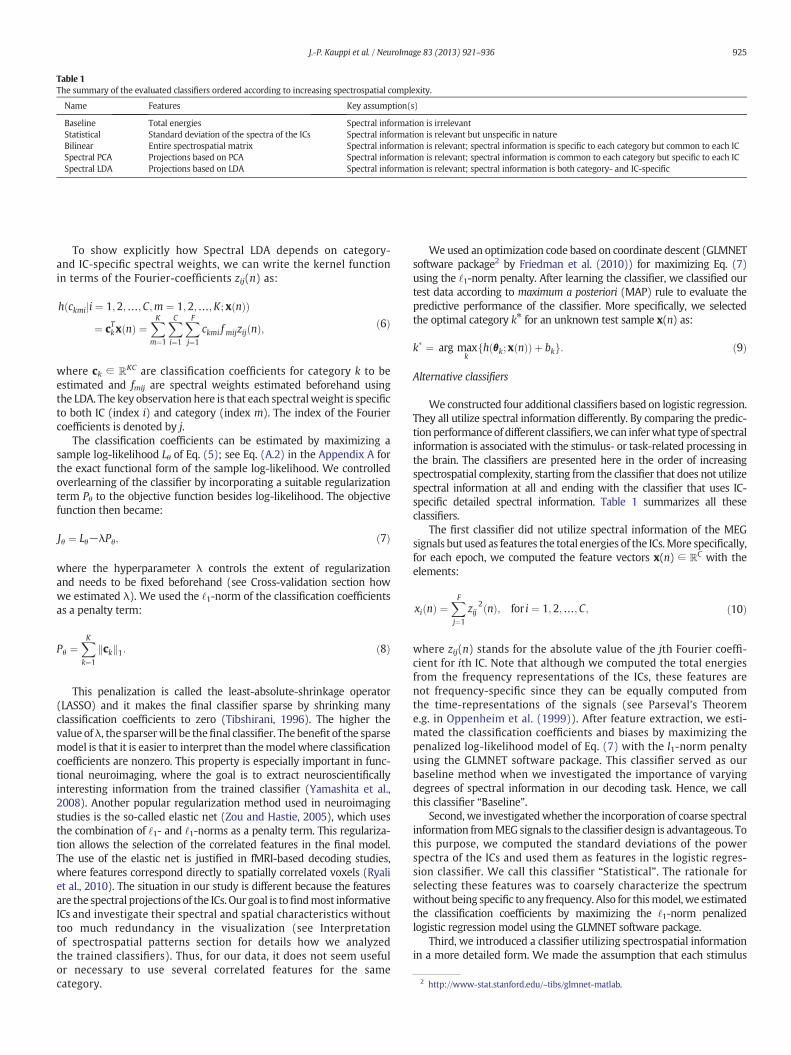
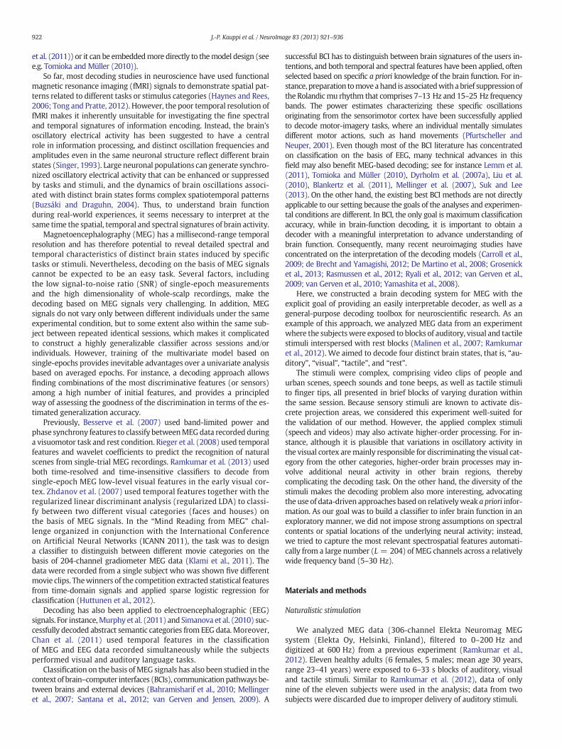
Table 1The summary of the evaluated classifiers ordered according to increasing spectrospatial complexity.

Name Features Key assumption(s)

Baseline Total energies Spectral information is irrelevantStatistical Standard deviation of the spectra of the ICs Spectral information is relevant but unspecific in natureBilinear Entire spectrospatial matrix Spectral information is relevant; spectral information is specific to each category but common to each ICSpectral PCA Projections based on PCA Spectral information is relevant; spectral information is common to each category but specific to each ICSpectral LDA Projections based on LDA Spectral information is relevant; spectral information is both category- and IC-specific

2 http://www-stat.stanford.edu/~tibs/glmnet-matlab.

925J.-P. Kauppi et al. / NeuroImage 83 (2013) 921–936

To show explicitly how Spectral LDA depends on category-and IC-specific spectral weights, we can write the kernel functionin terms of the Fourier-coefficients zij(n) as:

hðckmi i ¼ 1;2;…;C;m ¼ 1;2;…;K; x nð Þj Þ¼ cTkx nð Þ ¼

XKm¼1

XCi¼1

XFj¼1

ckmi f mijzij nð Þ; ð6Þ

where ck ∈ ℝKC are classification coefficients for category k to beestimated and fmij are spectral weights estimated beforehand usingthe LDA. The key observation here is that each spectralweight is specificto both IC (index i) and category (index m). The index of the Fouriercoefficients is denoted by j.

The classification coefficients can be estimated by maximizing asample log-likelihood Lθ of Eq. (5); see Eq. (A.2) in the Appendix A forthe exact functional form of the sample log-likelihood. We controlledoverlearning of the classifier by incorporating a suitable regularizationterm Pθ to the objective function besides log-likelihood. The objectivefunction then became:

Jθ ¼ Lθ−λPθ; ð7Þ

where the hyperparameter λ controls the extent of regularizationand needs to be fixed beforehand (see Cross-validation section howwe estimated λ). We used the ‘1-norm of the classification coefficientsas a penalty term:

Pθ ¼XKk¼1

ckk k1: ð8Þ

This penalization is called the least-absolute-shrinkage operator(LASSO) and it makes the final classifier sparse by shrinking manyclassification coefficients to zero (Tibshirani, 1996). The higher thevalue ofλ, the sparserwill be thefinal classifier. Thebenefit of the sparsemodel is that it is easier to interpret than themodel where classificationcoefficients are nonzero. This property is especially important in func-tional neuroimaging, where the goal is to extract neuroscientificallyinteresting information from the trained classifier (Yamashita et al.,2008). Another popular regularization method used in neuroimagingstudies is the so-called elastic net (Zou and Hastie, 2005), which usesthe combination of ‘1- and ‘1-norms as a penalty term. This regulariza-tion allows the selection of the correlated features in the final model.The use of the elastic net is justified in fMRI-based decoding studies,where features correspond directly to spatially correlated voxels (Ryaliet al., 2010). The situation in our study is different because the featuresare the spectral projections of the ICs. Our goal is tofindmost informativeICs and investigate their spectral and spatial characteristics withouttoo much redundancy in the visualization (see Interpretationof spectrospatial patterns section for details how we analyzedthe trained classifiers). Thus, for our data, it does not seem usefulor necessary to use several correlated features for the samecategory.

Weused an optimization code based on coordinate descent (GLMNETsoftware package2 by Friedman et al. (2010)) for maximizing Eq. (7)using the ‘1-norm penalty. After learning the classifier, we classified ourtest data according to maximum a posteriori (MAP) rule to evaluate thepredictive performance of the classifier. More specifically, we selectedthe optimal category k⁎ for an unknown test sample x(n) as:

k� ¼ arg maxk

h θk;x nð Þð Þ þ bkf g: ð9Þ

Alternative classifiers

We constructed four additional classifiers based on logistic regression.They all utilize spectral information differently. By comparing the predic-tionperformanceof different classifiers,we can inferwhat type of spectralinformation is associated with the stimulus- or task-related processing inthe brain. The classifiers are presented here in the order of increasingspectrospatial complexity, starting from the classifier that does not utilizespectral information at all and ending with the classifier that uses IC-specific detailed spectral information. Table 1 summarizes all theseclassifiers.

The first classifier did not utilize spectral information of the MEGsignals but used as features the total energies of the ICs.More specifically,for each epoch, we computed the feature vectors x(n) ∈ ℝC with theelements:

xi nð Þ ¼XFj¼1

zij2 nð Þ; for i ¼ 1;2;…;C; ð10Þ

where zij(n) stands for the absolute value of the jth Fourier coeffi-cient for ith IC. Note that although we computed the total energiesfrom the frequency representations of the ICs, these features arenot frequency-specific since they can be equally computed fromthe time-representations of the signals (see Parseval's Theoreme.g. in Oppenheim et al. (1999)). After feature extraction, we esti-mated the classification coefficients and biases by maximizing thepenalized log-likelihood model of Eq. (7) with the l1-norm penaltyusing the GLMNET software package. This classifier served as ourbaseline method when we investigated the importance of varyingdegrees of spectral information in our decoding task. Hence, we callthis classifier “Baseline”.

Second, we investigatedwhether the incorporation of coarse spectralinformation fromMEG signals to the classifier design is advantageous. Tothis purpose, we computed the standard deviations of the powerspectra of the ICs and used them as features in the logistic regres-sion classifier. We call this classifier “Statistical”. The rationale forselecting these features was to coarsely characterize the spectrumwithout being specific to any frequency. Also for thismodel,we estimatedthe classification coefficients by maximizing the ‘1-norm penalizedlogistic regression model using the GLMNET software package.

Third, we introduced a classifier utilizing spectrospatial informationin a more detailed form. We made the assumption that each stimulus

926 J.-P. Kauppi et al. / NeuroImage 83 (2013) 921–936

category is associated with its own spectral signature that can bedescribed by F spectral weights. This signature can be present in severalICs, and the contributions of each IC are captured by C classificationcoefficients. We used logistic regression with a bilinear kernel tobuild a classifier that fulfills these assumptions. A bilinear projection isgiven by:

h�cki; f kjji ¼ 1;2;…;C; j ¼ 1;2;…; F;Z nð Þ

�¼XCi¼1

XFj¼1

cki f kjzij nð Þ¼cTkZ nð Þfk;ð11Þ

where Z(n) ∈ ℝC × F is now an entire matrix given in Eq. (1), andck ∈ ℝC and fk ∈ ℝF denote the classification coefficients to be estimatedfor each category k, respectively. Now, each spectral classification coeffi-cient depends on the category (index k) but not on the IC (index i). Theindex of the Fourier coefficients is denoted by j. A bilinear formulation ofthe logistic regression has been discussed previously in the context of BCIunder the name bilinear component analysis (Dyrholm et al., 2007a).The learning of this classifier is feasible even from rather limited trainingdata, because the total number of parameters to be estimated is onlyK(C + F + 1) and not K(CF + 1) due to the assumption that spectralcoefficients and IC coefficients are separable. We call this classifier“Bilinear”. We used a conjugate gradient method3 by Rasmussenand Nickisch (2010) for maximizing the penalized log-likelihood,because the GLMNET software package cannot handle a bilinearkernel function. See Appendix A for details how we obtained thegradient and the objective function for this classifier.

Fourth, we used an unsupervised learning method which leads to aclassifier similar in spirit to Bilinear classifier. While Bilinear classifieris based on the mathematically attractive assumption that different ICsshare the same spectral characteristics for a given category, amore plau-sible assumption is that each IC can have unique spectral characteristics.To investigate whether the latter assumption would yield better pre-diction performance, we constructed a classifier for which we estimatedspectral-weight vectors for each IC separately before estimating theclassification coefficients of the ICs, somewhat like in Spectral LDA. Weapplied PCA to the short-time spectra of each IC and took the first princi-pal directions as the estimates for spectral weights. We formed featurevectors by projecting the short-time spectra to one dimension (similarto Spectral LDA, but now we computed only one projection per ICs)and estimated the classification coefficients and biases by maximizingthe ‘1-penalized logistic regression model of Eq. (7) using the GLMNETsoftware package. Since we used PCA to estimate the spectral-weightvectors, we call this classifier “Spectral PCA”. To show explicitly howSpectral PCA depends on the IC-specific spectral weights, we can writethe kernel function in the form:

h�ckiji ¼ 1;2;…C; x nð Þ

�¼XCi¼1

XFj¼1

cki f ijzij nð Þ ¼ cTkx nð Þ: ð12Þ

Here, ck ∈ ℝC are classification coefficients to be estimated for categoryk, fij are spectral weights estimated using the PCA beforehand,x(n) ∈ ℝC is a feature vector, j is the index of the Fourier coefficients,and i is the index of the ICs. Note that spectral weights are notcategory-specific since they do not depend on the category index unlikethe corresponding weights for Spectral LDA in Eq. (6) or for Bilinearin Eq. (11).

Fig. 2 illustrates the differences between Bilinear, Spectral PCA andSpectral LDA classifiers. All the classifiers assume that each category isrepresented by a specific combination of some of the ICs (the classifierfinds these informative combinations; here, for simplicity, the foundcombinations were expected to be the same for all three classifiers).However, the way the spectral-weight vectors are estimated depends

3 http://www.gaussianprocess.org/gpml/code/matlab/util/minimize.m.

on the classifier. The spectral weights reflect the importance of differentfrequencies in the classification and are illustrated by black solid curvesnext to the spatial patterns. The shapes of the weight vectors dependeither on the category (Bilinear), the estimated source (Spectral PCA),or both (Spectral LDA).

Cross-validation

We trained all the classifiers based on the penalized log-likelihoodobjective function, which involves selecting a suitable hyperparametervalue λ that controls the extent of regularization. One possibility toautomatically determine λ is to aim at the best decoding performanceas measured by CV. Conventional CV procedures were not directlyapplicable to our data because of the temporal dependencies betweensuccessive time windows. However, time windows in differentstimulus/rest blocks can be assumed to be rather independentdue to the sharp onsets and offsets of the blocks. Thus, we can avoidthe problem of temporal dependencies by using a “leave-one-block-out” CV procedure (Lemm et al., 2011). For this procedure, we used allepochs fromone block for classifier validation and the rest of the epochsextracted from all the other blocks for classifier training during one CVloop.We trained the classifier and evaluated its performance using eachtraining and validation folds for several values of λ, and selected thefinal value according to the highest average classification accuracyacross the results.

To avoid bias, we estimated ICs and spectral-weight vectors sepa-rately for each CV data set. This procedure increased considerably thecomputational cost of the classifier training but could still be performedin a reasonable time. After we had estimated the hyperparameter valuethrough CV,we trained the final classifierwith this value using the entiretraining data set. We emphasize that for this classifier we only used datafrom the first session for classifier training (including hyperparameterestimation through CV) and reserved the entire second session for eval-uating the performance of the classifiers. Hence, the data used in the finalperformance evaluation were independent from the training data.

Multisubject classifier

Decoding by utilizing data simultaneously from multiple subjectscould inform about the extent of across-subject similarities in the mod-ulation of brain activity.We carried out amultisubject decoding analysisby pooling the epochs of multiple subjects from both sessions and thenperforming the estimation of ICs, spectral feature extraction and classifi-er training as described previously. To assess the decoding performance,we carried out leave-one-subject-out analysis, i.e., we assessed the clas-sification accuracybased on the data set of one subjectwhichwas left outfrom the training data set. We trained and tested the classifier 9 times sothat each subject was left out once of the training data set, and computedthemean decoding performance across the test results. We balanced thenumber of category labels between the categories separately for eachsubject to ensure that we had the same number of epochs per categoryfor classifier training from each subject.

Interpretation of Spectral LDA

Interpretation of spectrospatial patterns

Spectral LDA offers a possibility to investigate how spectral charac-teristics of the rhythmic brain activity change according to stimuluscategories. Although the initial number of features in the model wasrelatively high (=256), LASSO forced the coefficients of the uselessand/or correlated features to zero, thereby considerably simplifyingthe interpretation of the classifiers.

We concentrated on the visualization of the ICs (both their spectraland spatial characteristics) which corresponded to the positive classifi-cation coefficients only. As explained earlier, it is plausible to assume

Fig. 2. Schematic illustration of the classifiers Bilinear, Spectral PCA and Spectral LDA. (A) A schematic brain with three estimated ICs. (B) Classifier Bilinear assumes the same spectral-weight vector for each IC within each category, but each category has unique weights (see the similarities and differences in the shapes of the weight vectors). (C) Spectral PCA assumesa unique weight vector for each IC but the vectors are shared across categories (see especially the shape of the vector of a shared pattern #3 that remains fixed across categories).(D) Spectral LDA is themost flexible classifier, as it assumes unique spectral-weight vectors for each IC, similar to Spectral PCA, but the spectral weights are also category-specific, similarto Bilinear: weights in the column denoted by 1 (or 2) are specific for discriminating category 1 (or 2) from the other categories. We assume that the classifier automatically capturescategory-specific spectral information by assigning positive classification coefficients to informative spectral projections (the two arrows emphasize the columns which are expectedto be associated with high positive classification coefficients).

927J.-P. Kauppi et al. / NeuroImage 83 (2013) 921–936

that a positive classification coefficient for some category is associatedwith those ICs and spectral weights that are estimated by discriminatingthe given category from the other categories (because LDA maximizesthe class separation in the projected space by definition). On the otherhand, because the decrease in the value of this same projection meansthat the given category becomes less probable with respect to othercategories, negative classification coefficients do not have interestinginterpretation in this model.

The spectral weights themselves can be either positive or nega-tive. A positive value of a certain frequency bin means that an in-crease in the power at this frequency band makes the category ofthe corresponding classification coefficient more probable. Similarly, anegative value means that a decrease in the power at this frequencyincreases the probability of the category. To make the interpretationof the results meaningful, we normalized all classification coefficientsand spectral weights by the standard deviation of the input data corre-sponding to each coefficient.

Across-subject cluster analysis

In Spectral LDA, each classification coefficient is associated with onespectrospatial pattern given by the corresponding IC. It is convenient tovisualize this pattern using three adjacent plots: one for the spatialpattern, one for the spectral-weight vector, and one for the real spec-trum. If the classifier contains several positive classification coefficients,it is obvious that the interpretation of thefindings becomes complicateddue to the high number of plots. For some subjects and categories,the number of positive classification coefficients was so low that the

findings were relatively easy to interpret. However, for other subjectsand categories, the number of positive classification coefficients washigher (e.g. more than 10), making the interpretation of the findingsmore difficult. One possible strategy to simplify interpretations is to in-vestigate features associated with the highest classification coefficientsonly. The drawback of this approach is that it is not always obviousthat high classification coefficients are related to the most interestingfindings. For instance, it is possible that some of the coefficients withhigh magnitude are related to suppression of noise whereas some coef-ficients with a lowmagnitude are related to neuroscientifically interest-ingphenomena (Blankertz et al., 2011). Perhaps amore reliable strategyfor simplifying the interpretation is to visualize the most consistentfeatures across subjects. To enhance such visualization, we designed aclustering procedure to find similar features across subjects for eachcategory. The procedure consisted of the following steps:

1. Construction of the similarity matrix:We first identified the spectral-weight vectors associated with posi-tive classification coefficients and pooled them across the classifiersof the subjects (separately for each category). Then, for each categoryk, we formed a similaritymatrix by computing the pairwise similaritiesbetween the weight vectors based on a cross-correlation sequence,that is, cross-correlations computed when one of the spectra isshifted towards lower and higher frequencies. We computed thecross-correlations to account for individual variability in peak fre-quencies in the rhythmic oscillatory activity. For each vector pairfm, fn (the subscripts of the category and IC are omitted here for con-venience), we computed the cross-correlations across the frequency

Fig. 3.Mean (SEM) classification accuracy across the subjects for the five classifiers:C1 = Baseline, C2 = Statistical, C3 = Bilinear, C4 = Spectral PCA, and C5 = SpectralLDA. The shown significance levels (marked by asterisks) refer to the comparison of theclassifiers against Baseline.

928 J.-P. Kauppi et al. / NeuroImage 83 (2013) 921–936

range [−2.5 Hz 2.5 Hz], and normalized the values so that the auto-correlations at zero lag were identically 1.0. We selected the maxi-mum value as the similarity value and set all the negative cross-correlations to zero because we were interested in positive correla-tions. Hence, the elements of the similarity matrix were numbersbetween zero and one given by:

hsim m;nð Þ ¼ max 0; max xcorr fm; fnð Þ½ �f g; ð13Þ

where xcorr() denotes the normalized cross-correlation sequencebetween the two vectors as described above.

2. Adding spatial constrains to clustering:We required that only spatially similar ICs can be clustered together.To this aim, we computed a spatial binary similarity matrix bythresholding themagnitudes of the spatial patterns of the ICs (corre-sponding to the pooled spectral-weight vectors) and investigatedpairwise whether the thresholded patterns overlapped. In this ma-trix, the value one denoted overlap between the patterns (at leastin one channel) and the value zero meant that the patterns did notoverlap. We also accounted for the hemispheric symmetry of thebrain by flipping one pattern from each pair across the midline intothe opposite hemisphere and investigated a possible overlap withanother pattern (and gave a value 1 also in the case of symmetric“overlap”). As a result, we obtained a binary matrix with elementsb(m, n) denoting the pairs of spatially similar ICs. We then weightedthe similarity matrix of the LDA weight vectors with this matrix andtransformed the resulting similarity matrix to a dissimilarity matrix.Hence, the elements of the final dissimilarity matrix used for cluster-ing were given by:

h m;nð Þ ¼ 1−hsim m;nð Þb m;nð Þ: ð14Þ

We constructed one dissimilarity matrix for each category.3. Clustering and post-processing:

We clustered the data based on the obtained dissimilarity matri-ces using the average-linkage agglomerative hierarchical cluster-ing algorithm (Hastie et al., 2009).4 A clustering cutoff valueand a threshold for the spatial patterns were manually adjustedso that the spectrospatial characteristics of different clusters becamevisible. After clustering, it was possible that clusters contained morethan one pattern from single subjects. To simplify interpretation,in each cluster we retained only the pattern corresponding tothe highest classification coefficient for each subject. Hence, afterpost-processing, the maximum number of spectrospatial patternsin each cluster was nine: one pattern per subject.

4. Visualization:We visualized the spectral-weight vectors and spatial patternswithin the clusters on top of each other using a distinct color foreach subject. To facilitate the overall interpretation of the findings,we sorted the clusters according to their size from the largest to thesmallest.

Results

Classification performance

Fig. 3 presents the mean classification accuracy of the classifiersacross subjects. Themean accuracy is shown together with the standarderror of mean (SEM). We report results obtained with 4-s windowlength and 2/3 window overlap, since these parameters yielded thehighest performance across all classifiers.5 Themean classification accu-racy for all classifiers was well above the chance level (0.25). Spectral

4 We used the implementation from the Statistics Toolbox of Matlab.5 This window parameter combination did not yield the highest accuracy for Spectral

LDA, but it was used to avoid bias in the comparison of the results.

LDA provided the best performance with the mean accuracy of 0.686(i.e., 68.6% of the epochs were correctly classified for the test data).The result was significantly higher (at α = 0.001, Bonferroni corrected)comparedwith that of Baseline (mean performance 0.546; paired t-test;p = 0.0002). Also the result of Spectral PCA (mean performance 0.659)was statistically significant (at α = 0.05, Bonferroni corrected) com-pared with that of Baseline (p = 0.0076). The corresponding resultof Bilinear (mean performance 0.629) was not statistically significantafter the Bonferroni correction (p = 0.0188). The result of SpectralLDA was significantly higher (at α = 0.05, Bonferroni corrected) in thecomparison against Bilinear (p = 0.0024) but not in the comparisonagainst Spectral PCA (p = 0.3198). The classifier Statistical performedconsiderably worse (mean performance 0.453) than any other classifier.

Fig. 4 shows the subject-wise classification results (ordered from thehighest to the lowest based on the classification accuracies of SpectralLDA). The classification accuracy varied considerably between individualsfor all classifiers. Note that Spectral LDA yielded relatively good perfor-mance for all subjects (the results varied between 0.485 and 0.838)whereas Spectral PCA yielded very good results for some subjects butrelatively poor results for some others (the results varied between0.382 and 0.882).

To test whether Spectral LDA would also work at single-individuallevel, we compared its classification accuracy with the performanceof a random classifier which assigns the data points to the classes ran-domly, with equal probabilities. The results of Spectral LDA were signif-icantly above the chance level (at α = 0.001, Bonferroni corrected) forall subjects (p b 8 × 10−6 for all the subjects); see Pereira et al. (2009)for details of the test.

Table 2 presents the confusion matrices of the classifiers, with therows denoting the true and the columns the estimated categories. TheSpectral LDA provided the highest mean classification accuracies forthe categories “auditory” (0.575) and “visual” (0.830). Bilinear yielded

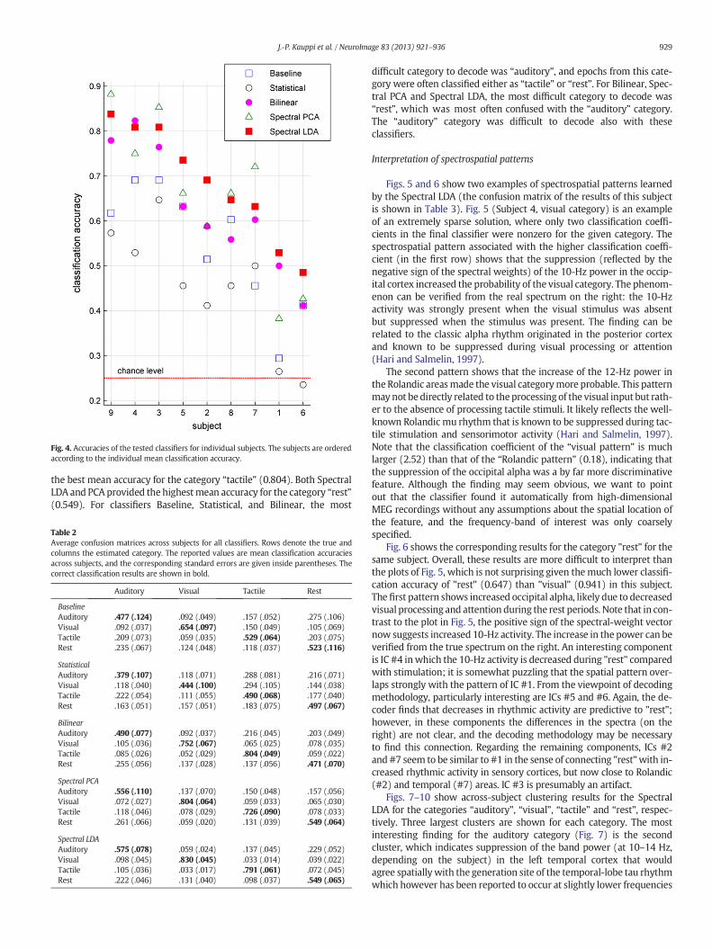
Fig. 4. Accuracies of the tested classifiers for individual subjects. The subjects are orderedaccording to the individual mean classification accuracy.

929J.-P. Kauppi et al. / NeuroImage 83 (2013) 921–936

the best mean accuracy for the category “tactile” (0.804). Both SpectralLDA and PCA provided the highestmean accuracy for the category “rest”(0.549). For classifiers Baseline, Statistical, and Bilinear, the most

Table 2Average confusion matrices across subjects for all classifiers. Rows denote the true andcolumns the estimated category. The reported values are mean classification accuraciesacross subjects, and the corresponding standard errors are given inside parentheses. Thecorrect classification results are shown in bold.

Auditory Visual Tactile Rest

BaselineAuditory .477 (.124) .092 (.049) .157 (.052) .275 (.106)Visual .092 (.037) .654 (.097) .150 (.049) .105 (.069)Tactile .209 (.073) .059 (.035) .529 (.064) .203 (.075)Rest .235 (.067) .124 (.048) .118 (.037) .523 (.116)

StatisticalAuditory .379 (.107) .118 (.071) .288 (.081) .216 (.071)Visual .118 (.040) .444 (.100) .294 (.105) .144 (.038)Tactile .222 (.054) .111 (.055) .490 (.068) .177 (.040)Rest .163 (.051) .157 (.051) .183 (.075) .497 (.067)

BilinearAuditory .490 (.077) .092 (.037) .216 (.045) .203 (.049)Visual .105 (.036) .752 (.067) .065 (.025) .078 (.035)Tactile .085 (.026) .052 (.029) .804 (.049) .059 (.022)Rest .255 (.056) .137 (.028) .137 (.056) .471 (.070)

Spectral PCAAuditory .556 (.110) .137 (.070) .150 (.048) .157 (.056)Visual .072 (.027) .804 (.064) .059 (.033) .065 (.030)Tactile .118 (.046) .078 (.029) .726 (.090) .078 (.033)Rest .261 (.066) .059 (.020) .131 (.039) .549 (.064)

Spectral LDAAuditory .575 (.078) .059 (.024) .137 (.045) .229 (.052)Visual .098 (.045) .830 (.045) .033 (.014) .039 (.022)Tactile .105 (.036) .033 (.017) .791 (.061) .072 (.045)Rest .222 (.046) .131 (.040) .098 (.037) .549 (.065)

difficult category to decode was “auditory”, and epochs from this cate-gory were often classified either as “tactile” or “rest”. For Bilinear, Spec-tral PCA and Spectral LDA, the most difficult category to decode was“rest”, which was most often confused with the “auditory” category.The “auditory” category was difficult to decode also with theseclassifiers.

Interpretation of spectrospatial patterns

Figs. 5 and 6 show two examples of spectrospatial patterns learnedby the Spectral LDA (the confusion matrix of the results of this subjectis shown in Table 3). Fig. 5 (Subject 4, visual category) is an exampleof an extremely sparse solution, where only two classification coeffi-cients in the final classifier were nonzero for the given category. Thespectrospatial pattern associated with the higher classification coeffi-cient (in the first row) shows that the suppression (reflected by thenegative sign of the spectral weights) of the 10-Hz power in the occip-ital cortex increased the probability of the visual category. The phenom-enon can be verified from the real spectrum on the right: the 10-Hzactivity was strongly present when the visual stimulus was absentbut suppressed when the stimulus was present. The finding can berelated to the classic alpha rhythm originated in the posterior cortexand known to be suppressed during visual processing or attention(Hari and Salmelin, 1997).

The second pattern shows that the increase of the 12-Hz power inthe Rolandic areasmade the visual categorymore probable. This patternmay not bedirectly related to theprocessing of the visual input but rath-er to the absence of processing tactile stimuli. It likely reflects the well-known Rolandic mu rhythm that is known to be suppressed during tac-tile stimulation and sensorimotor activity (Hari and Salmelin, 1997).Note that the classification coefficient of the “visual pattern” is muchlarger (2.52) than that of the “Rolandic pattern” (0.18), indicating thatthe suppression of the occipital alpha was a by far more discriminativefeature. Although the finding may seem obvious, we want to pointout that the classifier found it automatically from high-dimensionalMEG recordings without any assumptions about the spatial location ofthe feature, and the frequency-band of interest was only coarselyspecified.

Fig. 6 shows the corresponding results for the category "rest" for thesame subject. Overall, these results are more difficult to interpret thanthe plots of Fig. 5, which is not surprising given themuch lower classifi-cation accuracy of "rest" (0.647) than "visual" (0.941) in this subject.The first pattern shows increased occipital alpha, likely due to decreasedvisual processing and attention during the rest periods. Note that in con-trast to the plot in Fig. 5, the positive sign of the spectral-weight vectornow suggests increased 10-Hz activity. The increase in the power can beverified from the true spectrum on the right. An interesting componentis IC #4 inwhich the 10-Hz activity is decreased during "rest" comparedwith stimulation; it is somewhat puzzling that the spatial pattern over-laps strongly with the pattern of IC #1. From the viewpoint of decodingmethodology, particularly interesting are ICs #5 and #6. Again, the de-coder finds that decreases in rhythmic activity are predictive to "rest";however, in these components the differences in the spectra (on theright) are not clear, and the decoding methodology may be necessaryto find this connection. Regarding the remaining components, ICs #2and #7 seem to be similar to #1 in the sense of connecting "rest"with in-creased rhythmic activity in sensory cortices, but now close to Rolandic(#2) and temporal (#7) areas. IC #3 is presumably an artifact.

Figs. 7–10 show across-subject clustering results for the SpectralLDA for the categories “auditory”, “visual”, “tactile” and “rest”, respec-tively. Three largest clusters are shown for each category. The mostinteresting finding for the auditory category (Fig. 7) is the secondcluster, which indicates suppression of the band power (at 10–14 Hz,depending on the subject) in the left temporal cortex that wouldagree spatiallywith the generation site of the temporal-lobe tau rhythmwhich however has been reported to occur at slightly lower frequencies

Fig. 5. Spectrospatial patterns (ICs and their associated LDA weight vectors) found for Subject 4 for the category “auditory”. Rows denote all the found patterns in the order of decreasingclassification coefficients (the values of the classification coefficients are shownon the left), and columns denote the spectrospatial characteristics of each pattern: the spatial pattern of theIC on the sensor helmet viewed from left, back, and right (leftmost column), the LDAweight vector associatedwith the IC (middle column), and the “real” spectra of the IC at a logarithmicscale (rightmost column). In the rightmost column, the black color of the real spectrum denotes the average spectra computed across the epochs belonging to the category of interest, andthe red color indicates the corresponding spectrum computed across all the other categories. See Interpretation of spectrospatial patterns section on how to interpret themodel coefficients.

Fig. 6. Spectrospatial patterns found for Subject 4 for the category “rest”. See the captionof Fig. 5 for the meaning of the plots and Interpretation of spectrospatial patterns sectionon how to interpret the model coefficients.

930 J.-P. Kauppi et al. / NeuroImage 83 (2013) 921–936

of 8–10 Hz (Lehtelä et al., 1997). The first and the third clusters seem toshow increases in the Rolandic mu and occipital alpha rhythms, respec-tively. The signs of the spectral weights are plausible because the tactileand visual stimuli were not present.

The first cluster of the visual category (Fig. 8) indicates strong sup-pression of the occipital alpha rhythm, suggesting involvement of visualprocessing. The second cluster was also located in the posterior cortex,with increase in power in the 8–10 Hz band, implying that alpharhythms of different center frequencies may behave functionally differ-ently. The third cluster, withweak (0.09)weight overlapswith Rolandicareas and suggests suppression of the twomain frequency componentsof the mu rhythm.

The clusters of the tactile category (Fig. 9) were all located aroundthe Rolandic areas. The first cluster showed suppression at around10–13 Hz as well as at 19–22 Hz (however, one subject showed sup-pression already at 7 and 13 Hz). These findings could reflect suppres-sion of the Rolandic mu rhythm due to the tactile stimuli, here withconsiderably stronger weights than in the lowest panel of Fig. 8.Also the second and the third cluster indicated suppressed activity intwo distinct frequency bands, but the frequencies were lower than inthe first cluster (the approximate frequency bands were 6–10 Hz and14–17 Hz). Because the subjects of the second and third cluster weredifferent from those of the first cluster, also these findings may reflectRolandicmubutwith notable intersubject variation in the characteristicfrequencies. In any case, most of these findings agree with the currentliterature because the mu rhythm typically contains both 8–13 Hz and15–25 Hz frequency bands (Hari and Salmelin, 1997).

The largest cluster of the category “rest” (Fig. 10) showed variablespectral characteristics across a wide frequency band (5–25 Hz) inthe parietal cortex, mainly indicating increased oscillatory activity.This result may be related to increased Rolandic mu due to the absenceof tactile stimuli, or it might reflect spontaneous variations not related

Table 3The confusion matrix of the subject 4 whose spectrospatial features are shown in Figs. 5and 6. Rows denote the true and columns the estimated category memberships. The cor-rect classification results are shown in bold.

Subject 4 Auditory Visual Tactile Rest

Auditory .941 0 0.059 0Visual 0 .941 0.059 0Tactile 0.177 0.118 .706 0Rest 0.177 0.117 0.059 .647

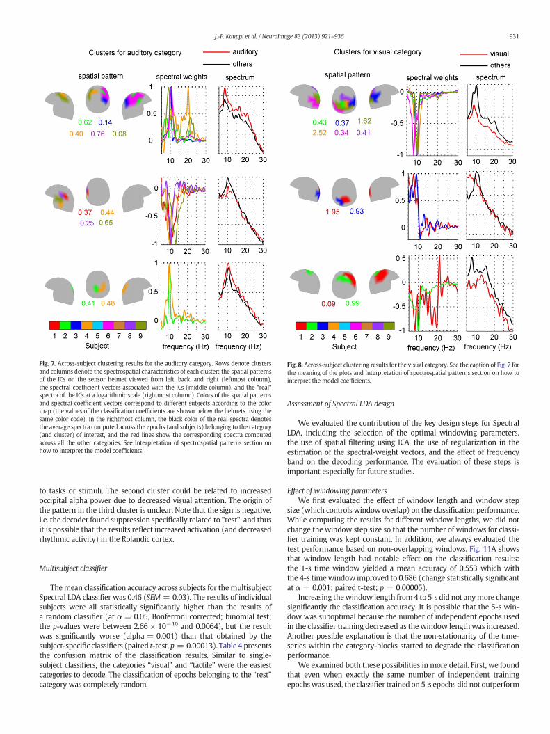
Fig. 7. Across-subject clustering results for the auditory category. Rows denote clustersand columns denote the spectrospatial characteristics of each cluster: the spatial patternsof the ICs on the sensor helmet viewed from left, back, and right (leftmost column),the spectral-coefficient vectors associated with the ICs (middle column), and the “real”spectra of the ICs at a logarithmic scale (rightmost column). Colors of the spatial patternsand spectral-coefficient vectors correspond to different subjects according to the colormap (the values of the classification coefficients are shown below the helmets using thesame color code). In the rightmost column, the black color of the real spectra denotesthe average spectra computed across the epochs (and subjects) belonging to the category(and cluster) of interest, and the red lines show the corresponding spectra computedacross all the other categories. See Interpretation of spectrospatial patterns section onhow to interpret the model coefficients.

Fig. 8. Across-subject clustering results for the visual category. See the caption of Fig. 7 forthe meaning of the plots and Interpretation of spectrospatial patterns section on how tointerpret the model coefficients.

931J.-P. Kauppi et al. / NeuroImage 83 (2013) 921–936

to tasks or stimuli. The second cluster could be related to increasedoccipital alpha power due to decreased visual attention. The origin ofthe pattern in the third cluster is unclear. Note that the sign is negative,i.e. the decoder found suppression specifically related to "rest", and thusit is possible that the results reflect increased activation (and decreasedrhythmic activity) in the Rolandic cortex.

Multisubject classifier

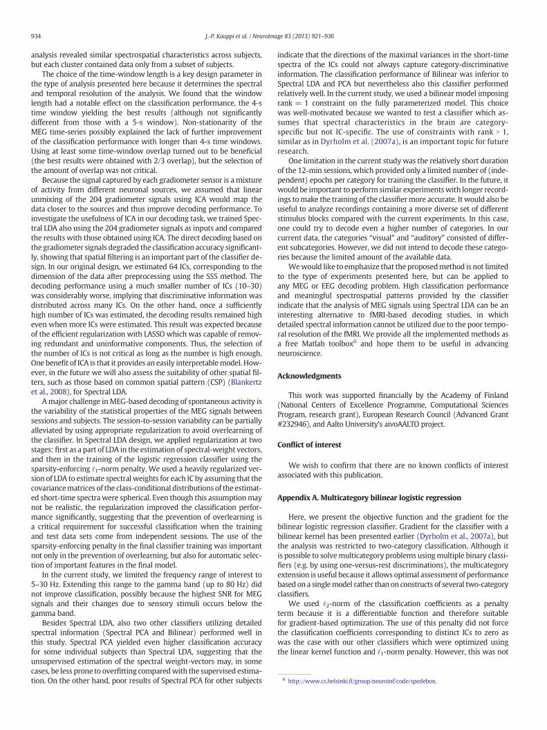
Themean classification accuracy across subjects for themultisubjectSpectral LDA classifier was 0.46 (SEM = 0.03). The results of individualsubjects were all statistically significantly higher than the results ofa random classifier (at α = 0.05, Bonferroni corrected; binomial test;the p-values were between 2.66 × 10−10 and 0.0064), but the resultwas significantly worse (alpha = 0.001) than that obtained by thesubject-specific classifiers (paired t-test, p = 0.00013). Table 4 presentsthe confusion matrix of the classification results. Similar to single-subject classifiers, the categories “visual” and “tactile” were the easiestcategories to decode. The classification of epochs belonging to the “rest”category was completely random.

Assessment of Spectral LDA design

We evaluated the contribution of the key design steps for SpectralLDA, including the selection of the optimal windowing parameters,the use of spatial filtering using ICA, the use of regularization in theestimation of the spectral-weight vectors, and the effect of frequencyband on the decoding performance. The evaluation of these steps isimportant especially for future studies.

Effect of windowing parametersWe first evaluated the effect of window length and window step

size (which controls window overlap) on the classification performance.While computing the results for different window lengths, we did notchange the window step size so that the number of windows for classi-fier training was kept constant. In addition, we always evaluated thetest performance based on non-overlapping windows. Fig. 11A showsthat window length had notable effect on the classification results:the 1-s time window yielded a mean accuracy of 0.553 which withthe 4-s timewindow improved to 0.686 (change statistically significantat α = 0.001; paired t-test; p = 0.00005).

Increasing thewindow length from 4 to 5 s did not anymore changesignificantly the classification accuracy. It is possible that the 5-s win-dow was suboptimal because the number of independent epochs usedin the classifier training decreased as the window length was increased.Another possible explanation is that the non-stationarity of the time-series within the category-blocks started to degrade the classificationperformance.

We examined both these possibilities in more detail. First, we foundthat even when exactly the same number of independent trainingepochswas used, the classifier trained on 5-s epochs did not outperform

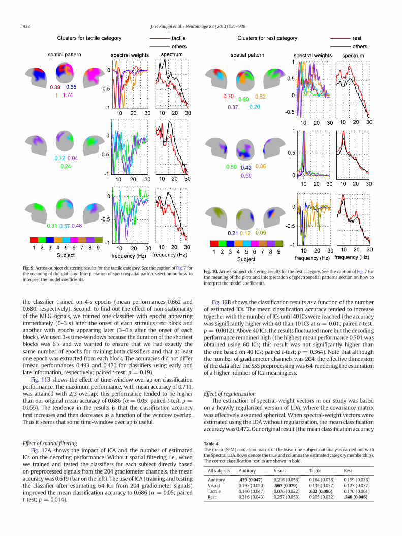
Fig. 9. Across-subject clustering results for the tactile category. See the caption of Fig. 7 forthe meaning of the plots and Interpretation of spectrospatial patterns section on how tointerpret the model coefficients.

Fig. 10. Across-subject clustering results for the rest category. See the caption of Fig. 7 forthe meaning of the plots and Interpretation of spectrospatial patterns section on how tointerpret the model coefficients.

932 J.-P. Kauppi et al. / NeuroImage 83 (2013) 921–936

the classifier trained on 4-s epochs (mean performances 0.662 and0.680, respectively). Second, to find out the effect of non-stationarityof the MEG signals, we trained one classifier with epochs appearingimmediately (0–3 s) after the onset of each stimulus/rest block andanother with epochs appearing later (3–6 s after the onset of eachblock). We used 3-s time-windows because the duration of the shortestblocks was 6 s and we wanted to ensure that we had exactly thesame number of epochs for training both classifiers and that at leastone epoch was extracted from each block. The accuracies did not differ(mean performances 0.493 and 0.470 for classifiers using early andlate information, respectively; paired t-test; p = 0.19).

Fig. 11B shows the effect of time-window overlap on classificationperformance. The maximum performance, with mean accuracy of 0.711,was attained with 2/3 overlap; this performance tended to be higherthan our original mean accuracy of 0.686 (α = 0.05; paired t-test, p =0.055). The tendency in the results is that the classification accuracyfirst increases and then decreases as a function of the window overlap.Thus it seems that some time-window overlap is useful.

Table 4The mean (SEM) confusion matrix of the leave-one-subject-out analysis carried out withthe Spectral LDA. Rowsdenote the true and columns the estimated categorymemberships.The correct classification results are shown in bold.

All subjects Auditory Visual Tactile Rest

Auditory .439 (0.047) 0.216 (0.056) 0.164 (0.036) 0.199 (0.036)Visual 0.193 (0.050) .567 (0.079) 0.135 (0.037) 0.123 (0.037)Tactile 0.140 (0.047) 0.076 (0.022) .632 (0.096) 0.170 (0.061)Rest 0.316 (0.043) 0.257 (0.053) 0.205 (0.032) .240 (0.046)

Effect of spatial filteringFig. 12A shows the impact of ICA and the number of estimated

ICs on the decoding performance. Without spatial filtering, i.e., whenwe trained and tested the classifiers for each subject directly basedon preprocessed signals from the 204 gradiometer channels, the meanaccuracywas 0.619 (bar on the left). The use of ICA (training and testingthe classifier after estimating 64 ICs from 204 gradiometer signals)improved the mean classification accuracy to 0.686 (α = 0.05; pairedt-test; p = 0.014).

Fig. 12B shows the classification results as a function of the numberof estimated ICs. The mean classification accuracy tended to increasetogether with the number of ICs until 40 ICswere reached (the accuracywas significantly higher with 40 than 10 ICs at α = 0.01; paired t-test;p = 0.0012). Above 40 ICs, the resultsfluctuatedmore but the decodingperformance remained high (the highest mean performance 0.701 wasobtained using 60 ICs; this result was not significantly higher thanthe one based on 40 ICs; paired t-test; p = 0.364). Note that althoughthe number of gradiometer channels was 204, the effective dimensionof the data after the SSS preprocessingwas 64, rendering the estimationof a higher number of ICs meaningless.

Effect of regularizationThe estimation of spectral-weight vectors in our study was based

on a heavily regularized version of LDA, where the covariance matrixwas effectively assumed spherical. When spectral-weight vectors wereestimated using the LDAwithout regularization, themean classificationaccuracywas0.472. Our original result (themean classification accuracy

Fig. 11. The effect of window parameters on the classification performance of SpectralLDA: (A) the effect of window length, and (B) the effect of window step size (presentedas fractions of the overlap between two successive windows). For instance, windowoverlap = 0 means that successive windows did not overlap at all (but are adjacent toeach other), and window overlap = 1/2 indicates 50% overlap between the successivewindows.

933J.-P. Kauppi et al. / NeuroImage 83 (2013) 921–936

0.686) was significantly better than the unregularized one at α = 0.001(paired t-test; p = 0.00026). The poor performance of the unregularizedLDA was not surprising, because the dimension of the short-time spectra

Fig. 12. The effect of ICA on the classification performance of Spectral LDA. A) meanclassification accuracieswithout (a left bar labeled as “chan.”) andwith (a right bar labeledas “ICs”) applying ICA to the 204 gradiometer signals. B) The effect of the estimated numberof ICs from 10 to 64 on the classification accuracy.

was roughly equal to the number epochs, making the estimation of theinverse of the covariance matrix unstable.

Effect of frequency rangeWe limited our analysis to frequencies below 30 Hz because we

assumed that higher frequencies might not be useful in our decodingtask due to their low SNR. Because the limit was arbitrary, we testedwhether the decoding accuracy would improve if we extended thefrequency range of interest to contain the gamma-band (frequenciesup to 80 Hz). The classification accuracy based on the 5–80-Hz range(mean performance 0.662) was not higher than based on our original5–30-Hz range (mean performance 0.686). The visual inspection ofthe LDA weight vectors verified that category-discriminative informa-tion was dominantly present below 30 Hz (the values of the weightsabove 30 Hz were zero or close to zero).

Discussion

In this paper, we introduced a novel general-purposeMEG decodingmethod, Spectral LDA, for the investigation of whole-brain rhythmicactivity during distinct conditions. We assessed the usefulness of themethod in a naturalistic setup comprising visual, auditory and tactilestimuli. Spectral LDA assumes that distinct brain activations (sources)are characterized by unique spectral patterns of cortical rhythms.Spectral LDA also assumes that the spectral patternsmay vary accordingto the brain state. Although these assumptions are rather obvious asfar as brain function is concerned (see e.g. Singer, 1993; Buzsáki andDraguhn, 2004), decoding of different brain states and different appliedstimuli from the very noisy and relatively short single-trialMEG traces isfar from trivial. However, Spectral LDA performed very well in thisdifficult task and was superior to three out of four classifiers based onmore restrictive assumptions concerning spectrospatial information inthe data (Figs. 3, 4; these three classifiers were Baseline, Statistical,and Bilinear). The better performance of Spectral LDA compared withBaseline implies the usefulness of the spectral content of MEG signalsin the given decoding task. In addition, detailed spectral informationwas more useful than unspecific spectral information (as SpectralLDA performed better than Statistical). The results also indicate thatit is wise to estimate spectral signatures separately for distinct ICsinstead of estimating a common spectral feature for each category andusing thatwith each IC (Spectral LDAwas better than Bilinear). SpectralPCA provided comparable classification accuracy with Spectral LDA, butthe visualization of the final results is more meaningful with SpectralLDA.

The investigation of the trained classifiers showed that the SpectralLDA can provide neuroscientifically relevant information about state-dependent changes of rhythmic brain activity. To make the investiga-tion of the spectrospatial features across subjects easier, we developeda clustering method that took into account some functional and ana-tomical differences across individuals. The cluster analysis revealedthat many subjects shared similar spectrospatial features (Figs. 7–10).The spatial patterns of the dominant clusters agreed with functionallymeaningful brain areas. Naturally, the verification of different findingswill require additional studieswith newdata sets collected froma largernumber of subjects. In any case, already these findings are neurophysi-ologically encouraging, because themethod seeks patterns in an explor-atory manner based on minimal a priori assumptions concerning thebrain areas and frequencies of interest.

The decoding performance of the classifier trained with the dataof several subjects and tested with a subject not included in the trainingdata showed that Spectral LDA was capable of utilizing commonspectrospatial features across subjects. However, the multisubject clas-sifier was not competitive against the single-subject classifiers,suggesting notable interindividual variation in the rhythmic brain activ-ity. Across-subject clustering results supported this view: cluster

6 http://www.cs.helsinki.fi/group/neuroinf/code/spedebox.

934 J.-P. Kauppi et al. / NeuroImage 83 (2013) 921–936

analysis revealed similar spectrospatial characteristics across subjects,but each cluster contained data only from a subset of subjects.

The choice of the time-window length is a key design parameter inthe type of analysis presented here because it determines the spectraland temporal resolution of the analysis. We found that the windowlength had a notable effect on the classification performance, the 4-stime window yielding the best results (although not significantlydifferent from those with a 5-s window). Non-stationarity of theMEG time-series possibly explained the lack of further improvementof the classification performance with longer than 4-s time windows.Using at least some time-window overlap turned out to be beneficial(the best results were obtained with 2/3 overlap), but the selection ofthe amount of overlap was not critical.

Because the signal captured by each gradiometer sensor is a mixtureof activity from different neuronal sources, we assumed that linearunmixing of the 204 gradiometer signals using ICA would map thedata closer to the sources and thus improve decoding performance. Toinvestigate the usefulness of ICA in our decoding task, we trained Spec-tral LDA also using the 204 gradiometer signals as inputs and comparedthe results with those obtained using ICA. The direct decoding based onthe gradiometer signals degraded the classification accuracy significant-ly, showing that spatial filtering is an important part of the classifier de-sign. In our original design, we estimated 64 ICs, corresponding to thedimension of the data after preprocessing using the SSS method. Thedecoding performance using a much smaller number of ICs (10–30)was considerably worse, implying that discriminative information wasdistributed across many ICs. On the other hand, once a sufficientlyhigh number of ICs was estimated, the decoding results remained higheven when more ICs were estimated. This result was expected becauseof the efficient regularization with LASSO which was capable of remov-ing redundant and uninformative components. Thus, the selection ofthe number of ICs is not critical as long as the number is high enough.One benefit of ICA is that it provides an easily interpretablemodel. How-ever, in the future we will also assess the suitability of other spatial fil-ters, such as those based on common spatial pattern (CSP) (Blankertzet al., 2008), for Spectral LDA.

Amajor challenge inMEG-based decoding of spontaneous activity isthe variability of the statistical properties of the MEG signals betweensessions and subjects. The session-to-session variability can be partiallyalleviated by using appropriate regularization to avoid overlearning ofthe classifier. In Spectral LDA design, we applied regularization at twostages:first as a part of LDA in the estimation of spectral-weight vectors,and then in the training of the logistic regression classifier using thesparsity-enforcing ‘1-norm penalty. We used a heavily regularized ver-sion of LDA to estimate spectral weights for each IC by assuming that thecovariancematrices of the class-conditional distributions of the estimat-ed short-time spectrawere spherical. Even though this assumptionmaynot be realistic, the regularization improved the classification perfor-mance significantly, suggesting that the prevention of overlearning isa critical requirement for successful classification when the trainingand test data sets come from independent sessions. The use of thesparsity-enforcing penalty in the final classifier training was importantnot only in the prevention of overlearning, but also for automatic selec-tion of important features in the final model.

In the current study, we limited the frequency range of interest to5–30 Hz. Extending this range to the gamma band (up to 80 Hz) didnot improve classification, possibly because the highest SNR for MEGsignals and their changes due to sensory stimuli occurs below thegamma band.

Besides Spectral LDA, also two other classifiers utilizing detailedspectral information (Spectral PCA and Bilinear) performed well inthis study. Spectral PCA yielded even higher classification accuracyfor some individual subjects than Spectral LDA, suggesting that theunsupervised estimation of the spectral weight-vectors may, in somecases, be less prone to overfitting comparedwith the supervised estima-tion. On the other hand, poor results of Spectral PCA for other subjects

indicate that the directions of the maximal variances in the short-timespectra of the ICs could not always capture category-discriminativeinformation. The classification performance of Bilinear was inferior toSpectral LDA and PCA but nevertheless also this classifier performedrelatively well. In the current study, we used a bilinear model imposingrank = 1 constraint on the fully parameterized model. This choicewas well-motivated because we wanted to test a classifier which as-sumes that spectral characteristics in the brain are category-specific but not IC-specific. The use of constraints with rank N 1,similar as in Dyrholm et al. (2007a), is an important topic for futureresearch.

One limitation in the current studywas the relatively short durationof the 12-min sessions, which provided only a limited number of (inde-pendent) epochs per category for training the classifier. In the future, itwould be important to perform similar experimentswith longer record-ings tomake the training of the classifiermore accurate. It would also beuseful to analyze recordings containing a more diverse set of differentstimulus blocks compared with the current experiments. In this case,one could try to decode even a higher number of categories. In ourcurrent data, the categories “visual” and “auditory” consisted of differ-ent subcategories. However, we did not intend to decode these catego-ries because the limited amount of the available data.

Wewould like to emphasize that the proposedmethod is not limitedto the type of experiments presented here, but can be applied toany MEG or EEG decoding problem. High classification performanceand meaningful spectrospatial patterns provided by the classifierindicate that the analysis of MEG signals using Spectral LDA can be aninteresting alternative to fMRI-based decoding studies, in whichdetailed spectral information cannot be utilized due to the poor tempo-ral resolution of the fMRI. We provide all the implemented methods asa free Matlab toolbox6 and hope them to be useful in advancingneuroscience.

Acknowledgments

This work was supported financially by the Academy of Finland(National Centers of Excellence Programme, Computational SciencesProgram, research grant), European Research Council (Advanced Grant#232946), and Aalto University's aivoAALTO project.

Conflict of interest

We wish to confirm that there are no known conflicts of interestassociated with this publication.

Appendix A. Multicategory bilinear logistic regression

Here, we present the objective function and the gradient for thebilinear logistic regression classifier. Gradient for the classifier with abilinear kernel has been presented earlier (Dyrholm et al., 2007a), butthe analysis was restricted to two-category classification. Although itis possible to solvemulticategory problems usingmultiple binary classi-fiers (e.g. by using one-versus-rest discriminations), the multicategoryextension is useful because it allows optimal assessment of performancebased on a singlemodel rather than on constructs of several two-categoryclassifiers.

We used ‘2-norm of the classification coefficients as a penaltyterm because it is a differentiable function and therefore suitablefor gradient-based optimization. The use of this penalty did not forcethe classification coefficients corresponding to distinct ICs to zero aswas the case with our other classifiers which were optimized usingthe linear kernel function and ‘1-norm penalty. However, this was not

935J.-P. Kauppi et al. / NeuroImage 83 (2013) 921–936

a major concern because we were solely interested in the predictionperformance (and not interpretability) of the bilinear classifier in thisstudy.

We found the gradients separately for the log-likelihood andthe penalty terms of the penalized objective function Jθ = Lθ − λPθ,and then computed the final gradient as ∇Jθ = ∇Lθ − λ∇Pθ. Thecomponents of the gradient of the penalty term are:

∂Pθ

∂cki¼

∂XK

k¼1ckk k22

� �∂cki

¼ 2cki: ðA:1Þ

For the bilinear classifier, observations are matrices Z(n). Under theassumptions that Z(n) are independent and category labels ynk follow amultinomial distribution with a parameter pk(Z(n)), the log-likelihoodof the symmetric logistic regression model is:

Lθ ¼1N

log∏N

n¼1∏K

k¼1pynkk Z nð Þð Þ ¼ 1

N

XNn¼1

XKk¼1

logeh θk ;Z nð Þð ÞþbkXKj¼1

eh θ j ;Z nð Þð Þþb j

0B@

1CA

ynk

¼ 1N

XNn¼1

XKk¼1

ynk h θk;Z nð Þð Þ þ bj

� �−

XKk¼1

ynk

!logXKj¼1

eh θ j ;Z nð Þð Þþb j

0@

1A

¼ 1N

XNn¼1

XKk¼1

ynk h θk;Z nð Þð Þ þ bj

� �− log

XKj¼1

eh θ j ;Z nð Þð Þþb j

0@

1A;

ðA:2Þ

where we have used knowledge that ∑ k = 1K ynk = 1. With bilinear

kernel function, Eq. (A.2) becomes:

Lθ ¼1N

XNn¼1

XKk¼1

ynk cTkZ nð Þfk þ bk� �

− logXkj¼1

ecTjZ nð Þ f jþb j

0@

1A; ðA:3Þ

and the elements of the gradient are partial derivatives of this functionwith respect to parameters ck, fk, and bk. These are given by:

∂Lθ∂cki

¼ 1N

XNn¼1

ynkXFj¼1

f kjzij nð Þ− ecTkZ nð Þ fkþbkXK

j¼1ec

TjZ nð Þ f jþb j

XFj¼1

f kjzij nð Þ

0B@

1CA

¼ 1N

XNn¼1

XFj¼1

f kjzij nð Þ ynk−pk Z nð Þð Þð ÞðA:4Þ

∂Lθ∂ f kj

¼ 1N

XNn¼1

ynkXCi¼1

ckizij nð Þ− ecTkZ nð Þ fkþbkXK

j¼1ec

TjZ nð Þ f jþb j

XCi¼1

ckizij nð Þ

0B@

1CA

¼ 1N

XNn¼1

XCi¼1

ckizij nð Þ ynk−pk Z nð Þð Þð ÞðA:5Þ

∂Lθ∂bk

¼ 1N

XNn¼1

ynk−pk Z nð Þð Þð Þ; ðA:6Þ

where zij(n) are the elements of the matrix Z(n).

References

Anemüller, J., Sejnowski, T.J., Makeig, S., 2003. Complex independent component analysisof frequency-domain electroencephalographic data. Neural Networks 16, 1311–1323.

Bahramisharif, A., Van Gerven, M., Heskes, T., Jensen, O., 2010. Covert attention allowsfor continuous control of brain–computer interfaces. Eur. J. Neurosci. 31, 1501–1508.

Besserve, M., Jerbi, K., Laurent, F., Baillet, S., Martinerie, J., Garnero, L., 2007. Classificationmethods for ongoing EEG and MEG signals. Biol. Res. 40, 415–437.

Bingham, E., Hyvärinen, A., 2000. A fast fixed-point algorithm for independent componentanalysis of complex valued signals. Int. J. Neural Syst. 10, 1–8.

Blankertz, B., Tomioka, R., Lemm, S., Kawanabe, M., Müller, K.R., 2008. Optimizing spatialfilters for robust EEG single-trial analysis. IEEE Signal Process. Mag. 25, 41–56.

Blankertz, B., Lemm, S., Treder, M., Haufe, S., Müller, K.R.R., 2011. Single-trial analysis andclassification of ERP components — a tutorial. NeuroImage 56, 814–825.

Buzsáki, G., Draguhn, A., 2004. Neuronal oscillations in cortical networks. Science 304,1926–1929.

Carroll, M.K., Cecchi, G.A., Rish, I., Garg, R., Rao, A.R., 2009. Prediction and interpretation ofdistributed neural activity with sparse models. NeuroImage 44, 112–122.

Chan, A.M., Halgren, E., Marinkovic, K., Cash, S.S., 2011. Decoding word and category-specific spatiotemporal representations from MEG and EEG. NeuroImage 54,3028–3039.

Cox, D.D., Savoy, R.L., 2003. Functional magnetic resonance imaging (fMRI) brain reading:detecting and classifying distributed patterns of fMRI activity in human visual cortex.NeuroImage 19, 261–270.

de Brecht, M., Yamagishi, N., 2012. Combining sparseness and smoothness improvesclassification accuracy and interpretability. NeuroImage 60, 1550–1561.

De Martino, F., Valente, G., Staeren, N.l., Ashburner, J., Goebel, R., Formisano, E., 2008.Combining multivariate voxel selection and support vector machines for mappingand classification of fMRI spatial patterns. NeuroImage 43, 44–58.

Dyrholm, M., Christoforou, C., Parra, L.C., 2007a. Bilinear discriminant component analysis.J. Mach. Learn. Res. 8, 1097–1111.

Dyrholm, M., Makeig, S., Hansen, L.K., 2007b. Model selection for convolutive ICAwith an application to spatiotemporal analysis of EEG. Neural Comput. 19,934–955.

Friedman, J.H., Hastie, T., Tibshirani, R., 2010. Regularization paths for generalized linearmodels via coordinate descent. J. Stat. Softw. 33, 1–22.

Grosenick, L., Klingenberg, B., Katovich, K., Knutson, B., Taylor, J.E., 2013. Interpretablewhole-brain prediction analysis with GraphNet. NeuroImage 72, 304–321.

Hari, R., Kujala, M.V., 2009. Brain basis of human social interaction: from concepts to brainimaging. Physiol. Rev. 89, 453–479.

Hari, R., Salmelin, R., 1997. Human cortical oscillations: a neuromagnetic view throughthe skull. Trends Neurosci. 20, 44–49.

Hasson, U., Nir, Y., Levy, I., Fuhrmann, G., Malach, R., 2004. Intersubject synchronization ofcortical activity during natural vision. Science 303, 1634–1640.

Hasson, U., Furman, O., Clark, D., Dudai, Y., Davachi, L., 2008. Enhanced intersubject corre-lations duringmovie viewing correlate with successful episodic encoding. Neuron 57,452–462.

Hastie, T., Tibshirani, R., Friedman, J., 2009. The Elements of Statistical Learning: DataMining, Inference, and Prediction, 2nd edition. Springer, New York.

Haynes, J.D., Rees, G., 2006. Decodingmental states from brain activity in humans. NatureRev. Neurosci. 7, 523–534.

Hejnar, M.P., Kiehl, K.A., Calhoun, V.D., 2007. Interparticipant correlations: a model freefMRI analysis technique. Hum. Brain Mapp. 28, 860–867.

Huttunen, H., Manninen, T., Kauppi, J.P., Tohka, J., 2012. Mind reading with regularizedmultinomial logistic regression. Mach. Vision Appl. 2012, 1–15.

Hyvärinen, A., Ramkumar, P., Parkkonen, L., Hari, R., 2010. Independent component analy-sis of short-time Fourier transforms for spontaneous EEG/MEG analysis. NeuroImage49, 257–271.

Kamitani, Y., Tong, F., 2005. Decoding the visual and subjective contents of the humanbrain. Nature Neurosci. 8, 679–685.

Kauppi, J.P., Jääskeläinen, I.P., Sams, M., Tohka, J., 2010. Inter-subject correlation of brainhemodynamic responses duringwatchingamovie: localization in space and frequency.Front. Neuroinform. 4, 5 (10 pp.).

Kauppi, J.P., Huttunen, H., Korkala, H., Jääskeläinen, I.P., Sams, M., Tohka, J., 2011. Faceprediction from fMRI data during movie stimulus: strategies for feature selection.Artif Neural Networks and Mach Learn — ICANN. Springer, pp. 189–196.

Klami, A., Ramkumar, P., Virtanen, S., Parkkonen, L., Hari, R., Kaski, S., 2011. ICANN/PASCAL2 challenge: MEG mind reading — overview and results. Proceedingsof ICANN/PASCAL2 Challenge: MEG Mind Reading. Aalto University Publicationseries SCIENCE + TECHNOLOGY 29/2011 Espoo, Finland, pp. 3–19.

Kriegeskorte, N., 2011. Pattern-information analysis: from stimulus decoding tocomputational-model testing. NeuroImage 56, 411–421.

Lahnakoski, J.M., Glerean, E., Salmi, J., Jääskeläinen, I.P., Sams, M., Hari, R., Nummenmaa, L.,2012. Naturalistic fMRI mapping reveals superior temporal sulcus as the hubfor the distributed brain network for social perception. Front. Hum. Neurosci. 6, 233(14 pp.).

Lehtelä, L., Salmelin, R., Hari, R., 1997. Evidence for reactive magnetic 10-Hz rhythm in thehuman auditory cortex. Neurosci. Lett. 222, 111–114.

Lemm, S., Blankertz, B., Dickhaus, T., Müller, K.R., 2011. Introduction to machine learningfor brain imaging. NeuroImage 56, 387–399.

Liu, G., Huang, G., Meng, J., Zhu, X., 2010. A frequency-weighted method combined withcommon spatial patterns for electroencephalogram classification in brain–computerinterface. Biomed. Signal Process. 5, 174–180.

Malinen, S., Hlushchuk, Y., Hari, R., 2007. Towards natural stimulation in fMRI — issues ofdata analysis. NeuroImage 35, 131–139.

Mellinger, J., Schalk, G., Braun, C., Preissl, H., Rosenstiel, W., Birbaumer, N., Kübler, A.,2007. An MEG-based brain–computer interface (BCI). NeuroImage 36, 581–593.

Mitchell, T.M., Hutchinson, R., Niculescu, R.S., Pereira, F., Wang, X., Just, M.A., Newman,S.D., 2004. Learning to decode cognitive states from brain images. Mach. Learn. 57,145–175.

Murphy, B., Poesio, M., Bovolo, F., Bruzzone, L., Dalponte, M., Lakany, H., 2011. EEGdecoding of semantic category reveals distributed representations for single concepts.Brain Lang. 117, 12–22.

Oppenheim, A.V., Schafer, R.W., Buck, J.R., et al., 1999. Discrete-Time Signal Processing,vol. 5. Prentice Hall, Upper Saddle River.

Pereira, F., Mitchell, T., Botvinick, M., 2009. Machine learning classifiers and fMRI: atutorial overview. NeuroImage 45, S199–S209.

Pfurtscheller, G., Neuper, C., 2001. Motor imagery and direct brain–computer communi-cation. IEEE Proc. 89, 1123–1134.

Ramkumar, P., Parkkonen, L., Hari, R., Hyvärinen, A., 2012. Characterization ofneuromagnetic brain rhythms over time scales of minutes using spatial independentcomponent analysis. Hum. Brain Mapp. 33, 1648–1662.

936 J.-P. Kauppi et al. / NeuroImage 83 (2013) 921–936

Ramkumar, P., Jas, M., Pannasch, S., Hari, R., Parkkonen, L., 2013. Feature-specific informa-tion processing precedes concerted activation in human visual cortex. J. Neurosci. 33,7691–7699.

Rasmussen, C.E., Nickisch, H., 2010. Gaussian processes for machine learning (GPML)toolbox. J. Mach. Learn. Res. 11, 3011–3015.

Rasmussen, P.M., Hansen, L.K., Madsen, K.H., Churchill, N.W., Strother, S.C., 2012. Modelsparsity and brain pattern interpretation of classification models in neuroimaging.Pattern Recogn. 45, 2085–2100.

Richiardi, J., Eryilmaz, H., Schwartz, S., Vuilleumier, P., Van De Ville, D., 2011. Decodingbrain states from fMRI connectivity graphs. NeuroImage 56, 616–626.

Rieger, J.W., Reichert, C., Gegenfurtner, K.R., Noesselt, T., Braun, C., Heinze, H.J.J., Kruse, R.,Hinrichs, H., 2008. Predicting the recognition of natural scenes from single trial MEGrecordings of brain activity. NeuroImage 42, 1056–1068.

Ryali, S., Supekar, K., Abrams, D.A., Menon, V., 2010. Sparse logistic regression for wholebrain classification of fMRI data. NeuroImage 51, 752–764.

Ryali, S., Chen, T., Supekar, K., Menon, V., 2012. Estimation of functional connectivityin fMRI data using stability selection-based sparse partial correlation with elasticnet penalty. NeuroImage 59, 3852–3861.

Santana, R., Bielza, C., Larrañaga, P., 2012. Regularized logistic regression and multiobjectivevariable selection for classifying MEG data. Biol. Cybern. 106, 389–405.

Simanova, I., van Gerven, M., Oostenveld, R., Hagoort, P., 2010. Identifying objectcategories from event-related EEG: toward decoding of conceptual representations.PloS One 5, e14465 (12 pp.).

Singer, W., 1993. Synchronization of cortical activity and its putative role in informationprocessing and learning. Annu. Rev. Physiol. 55, 349–374.

Spiers, H., Maguire, E., 2007. Decoding human brain activity during real-world experiences.Trends Cogn. Sci. 11, 356–365.

Suk, H.I., Lee, S.W., 2013. A novel Bayesian framework for discriminative featureextraction in brain–computer interfaces. IEEE Trans. Pattern Anal. Mach. Intell. 35,286–299.

Taulu, S., Kajola, M., 2005. Presentation of electromagnetic multichannel data: The signalspace separation method. J. Appl. Phys. 97, 124905 (10 pp.).

Tibshirani, R., 1996. Regression shrinkage and selection via the LASSO. J. R. Stat. Soc. Series B(Stat. Meth.) 58, 267–288.

Tomioka, R., Müller, K.R., 2010. A regularized discriminative framework for EEG analysiswith application to brain–computer interface. NeuroImage 49, 415–432.

Tong, F., Pratte, M.S., 2012. Decoding patterns of human brain activity. Annu. Rev. Psychol.63, 483–509.

van Gerven, M., Jensen, O., 2009. Attention modulations of posterior alpha as a controlsignal for two-dimensional brain–computer interfaces. J. Neurosci. Methods 179, 78–84.

van Gerven, M., Hesse, C., Jensen, O., Heskes, T., 2009. Interpreting single trial data usinggroupwise regularisation. NeuroImage 46, 665–676.

van Gerven, M.A., Cseke, B., De Lange, F.P., Heskes, T., 2010. Efficient Bayesian multivariatefMRI analysis using a sparsifying spatio-temporal prior. NeuroImage 50, 150–161.

Wolf, I., Dziobek, I., Heekeren, H.R., 2010. Neural correlates of social cognition in naturalisticsettings: a model-free analysis approach. NeuroImage 49, 894–904.

Yamashita, O., Sato, M.A., Yoshioka, T., Tong, F., Kamitani, Y., 2008. Sparse estimationautomatically selects voxels relevant for the decoding of fMRI activity patterns.NeuroImage 42, 1414–1429.

Zhdanov, A., Hendler, T., Ungerleider, L., Intrator, N., 2007. Inferring functional brain statesusing temporal evolution of regularized classifiers. Comput. Intell. Neurosci. 52609 (8pp.).

Zou, H., Hastie, T., 2005. Regularization and variable selection via the elastic net. J. R. Stat.Soc. Series B (Stat. Meth.) 67, 301–320.