Decomposing ERP time–frequency energy using PCA

Edward M. Bernata,*, William J. Williamsb,1, William J. Gehringc

aDepartment of Psychology, University of Minnesota, 75 East River Road, Elliot Hall, Minneapolis, MN 55455, USAbDepartment of EECS, University of Michigan, Ann Arbor, MI, USA

cDepartment of Psychology, University of Michigan, Ann Arbor, MI, USA

Accepted 26 January 2005

Available online 2 April 2005

Abstract

Objective: Time–frequency transforms (TFTs) offer rich representations of event-related potential (ERP) activity, and thus add complexity.

Data reduction techniques for TFTs have been slow to develop beyond time analysis of detail functions from wavelet transforms. Cohen’s

class of TFTs based on the reduced interference distribution (RID) offer some benefits over wavelet TFTs, but do not offer the simplicity of

detail functions from wavelet decomposition. The objective of the current approach is a data reduction method to extract succinct and

meaningful events from both RID and wavelet TFTs.

Methods: A general energy-based principal components analysis (PCA) approach to reducing TFTs is detailed. TFT surfaces are first

restructured into vectors, recasting the data as a two-dimensional matrix amenable to PCA. PCA decomposition is performed on the two-

dimensional matrix, and surfaces are then reconstructed. The PCA decomposition method is conducted with RID and Morlet wavelet TFTs,

as well as with PCA for time and frequency domains separately.

Results: Three simulated datasets were decomposed. These included Gabor logons and chirped signals. All simulated events were

appropriately extracted from the TFTs using both wavelet and RID TFTs. Varying levels of noise were then added to the simulated data, as

well as a simulated condition difference. The PCA-TFT method, particularly when used with RID TFTs, appropriately extracted the

components and detected condition differences for signals where time or frequency domain analysis alone failed. Response-locked ERP data

from a reaction time experiment was also decomposed. Meaningful components representing distinct neurophysiological activity were

extracted from the ERP TFT data, including the error-related negativity (ERN).

Conclusions: Effective TFT data reduction was achieved. Activity that overlapped in time, frequency, and topography were effectively

separated and extracted. Methodological issues involved in the application of PCA to TFTs are detailed, and directions for further

development are discussed.

Significance: The reported decomposition method represents a natural but significant extension of PCA into the TFT domain from the time

and frequency domains alone. Evaluation of many aspects of this extension could now be conducted, using the PCA-TFT decomposition as a

basis.

q 2005 Published by Elsevier Ireland Ltd. on behalf of International Federation of Clinical Neurophysiology.

Keywords: Time–frequency; Wavelet; ERP; Decomposition; Method

Methods for generating time–frequency transforms

(TFTs) have advanced greatly in recent years, producing

beautiful and complex ERP signal representations. This

advance in methods to create these representations has

increased the need for new data reduction methods to

1388-2457/$30.00 q 2005 Published by Elsevier Ireland Ltd. on behalf of Intern

doi:10.1016/j.clinph.2005.01.019

* Corresponding author. Tel.: C1 612 624 5063; fax: C1 612 626 2079.

E-mail address: ebernat@umn.edu (E.M. Bernat).1 Commercial interests: The second author is an owner of Quantum

Signal, the company that produces the Time–Frequency Toolbox.

parameterize them succinctly for analysis. TFTs are signal

processing techniques that permit the representation of

biological signals jointly in the time and frequency domains.

TFTs offer rich representations of electroencephalogram

(EEG) and event-related potential (ERP) activity, and

EEG/ERP work based on TFTs has begun to accelerate

dramatically in recent years. Williams et al. (1995), for

example, demonstrated advances in the use of TFTs in

identifying Epilepsy related EEG components during

seizures. Durka and Blinowska (2001), using the wavelet

Clinical Neurophysiology 116 (2005) 1314–1334

www.elsevier.com/locate/clinph

ational Federation of Clinical Neurophysiology.

E.M. Bernat et al. / Clinical Neurophysiology 116 (2005) 1314–1334 1315

Matching Pursuit algorithm (Mallat and Zhang, 1993) on

sleep EEG data, demonstrated that TFTs of EEG signals can

be more sensitive to experimental manipulations than

standard time-based EEG measures. Demiralp et al.

(1999) have shown that wavelet TFTs of ERP signals can

contain information not available using conventional ERP

analysis methods. Many others have advanced similar

arguments concerning the use of TFTs with EEG and ERP

signals (e.g. Basar et al., 1999; Morgan and Gevins, 1986;

Raz et al., 1999; Samar et al., 1995). However, because TFT

representations contain an additional dimension (joint time–

frequency versus time or frequency alone), they create

two-dimensional surfaces instead of single-dimension

waveforms. These surface representations generally create

a substantial increase in information. Reducing this

increased information in the TFT into a set of parameters

characterizing meaningful activity is more complex than in

the time or frequency domains alone. The problem is

something like identifying objects in a digitized photo-

graphic image. To look at the image one can often identify

the number and types of objects. However, to algorithmi-

cally identify the primary and consistent objects from

hundreds or thousands of such images taken from different

distances and angles is much more difficult. This problem is

compounded when higher resolution digital images are

used. On the one hand, the higher resolution offers the

possibility of resolving smaller objects, but this increases

the problem of identifying them because of the increased

number of data points in the image. Because TFT surface

representations of ERP data are somewhat new, and because

they are generally more complex, data reduction methods

have not yet been not well developed for them. Thus, there

is a growing need for new data reduction methods that can

accurately parameterize the activity in time–frequency

surface representations of ERPs, particularly those with

higher resolution. The method presented here is intended to

contribute towards that end.

The majority of recent EEG/ERP TFT work has been

done with wavelet transforms. In addition to wavelets,

advanced members of Cohen’s class of TFTs have been

employed (Cohen, 1989, 1992, 1995), specifically the

reduced interference distribution (RID, Williams, 1996,

2001; Williams et al., 1995). While wavelet methods are

well developed, some limitations of wavelets relative to

Cohen’s class suggest that further development of EEG/

ERP methods compatible with the RID may provide

additional analytic power. A more detailed description of

the differences is undertaken below, however, a primary

difference is that wavelets represent time–frequency energy

in frequency ranges defined by scales. A primary method of

analysis used with wavelet TFTs break the signal using the

different scales, and assess the associated time dependent

activity. RID TFTs, on the other hand, do not inherently

group energy across ranges of frequencies, instead provid-

ing the same sensitivity for all ranges of time and frequency

by calculating instantaneous frequency. This increased

sensitivity provides additional specificity (resolution) to

the time–frequency representation, and thus increases the

difficulty of parameterizing the information in the TFT for

analysis. The data reduction method detailed here is an

energy-based principal components analysis (PCA)

approach. It constitutes a general time–frequency data

reduction method for extracting joint time–frequency

components from TFTs. In this section, some important

differences between wavelet and Cohen’s class TFT

methods are highlighted (the reader is referred elsewhere

for thorough reviews of these methods), other methods for

TFT data reduction are discussed, and then the rationale for

the proposed method is provided.

1. Two primary TFT methods: wavelets and Cohen’s

class

Signal processing theory on TFT methods has advanced

in recent years. Two main classes of these TFT methods

have now been substantially developed: Cohen’s class (see

e.g. Cohen, 1989, 1992, 1995) and multiresolution analysis

or wavelets (see e.g. Daubechies, 1990; Graps, 1995;

Torrence and Compo, 1998; or as described specifically for

application to EEG/ERP, Samar et al., 1995, 1999a).

Cohen’s class is a general approach to TFTs, where an

infinite number of different kernel functions with different

constraints can be substituted in the main equation, creating

the members of the class (for a detailed description of the

role of kernels the reader is directed to Cohen, 1995). Some

specific examples of Cohen’s class TFTs (described in more

detail below) are the spectrogram, Wigner distribution, and

more recently the reduced interference distributions (RIDs)

such as the Choi-Williams (Choi and Williams, 1989) and

Binomial (Jeong and Williams, 1991). Cohen’s class TFTs

are generally referred to as time–frequency distributions

(TFDs), where distribution refers to an energy density

function or the associated distribution of time–frequency

energy. Wavelet approaches decompose signals into

constituent ranges of time–frequency energy (sometimes

referred to as tiles) based on scale (described below), using a

set of basis functions (see e.g. Samar et al., 1999a). An

infinite number of wavelet functions can be substituted in

the process, offering sensitivity to different types of activity.

Both methods are capable of producing high-resolution

TFTs, but they differ significantly in their approach,

implementation, and the inferences that can be drawn

from the resulting transforms. Appendix briefly presents a

more mathematical treatment of the RID TFD methodology

for the interested reader.

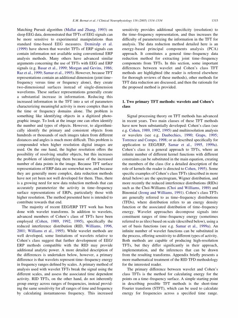
The primary difference between wavelet and Cohen’s

class TFTs is the method for calculating energy for the

points on a time–frequency surface. A simple starting point

in describing possible TFT methods is the short-time

Fourier transform (STFT), which can be used to calculate

energy for frequencies across a specified time range.

f

f

f

t

t

t

(a) Spectrogram windows

(b) Wavelet/scalogram windows

(c) Possible Cohen's class windows (RID)

Fig. 1. A comparison of windows for various analysis schemes. (a)

Spectrogram, (b) wavelet, (c) RID. Note that the spectrogram and RID

windows do not change shape with frequency, whereas the wavelet window

does. (Reproduced from Williams, 2001).

E.M. Bernat et al. / Clinical Neurophysiology 116 (2005) 1314–13341316

A series of STFTs can be calculated across time to create a

spectrogram to represent time–frequency energy. The main

problem with this approach is the fundamental tradeoff

between sensitivity in time and sensitivity in frequency that

is directly related to the length of the STFT window used

(the uncertainty principle). As a result, the STFT and

spectrogram cannot be sensitive to many different types of

signals simultaneously (Cohen, 1992; Samar et al., 1999a).

1.1. Wavelets

Wavelets provide an advance over the spectrogram by

application of a rational system for defining window sizes

that maximize sensitivity at different frequencies. This is

accomplished by utilizing the concept of scale in place of

frequency when defining varying window sizes for different

ranges of time–frequency activity. Levels of scale are often

described in terms of different resolutions of a landscape. At

the lowest resolution, only slow hills of the terrain might be

visible. At a medium resolution only buildings and fences

might be visible. At the highest resolution, only the blades

of grass or leaves of bushes might be visible. The

decomposition of the signal into constituent signals with

different resolutions is the basis for the name ‘multi-

multiresolution analysis’ that can be applied to wavelet

transforms.

Two broad classes of wavelet analyses are the discrete

wavelet transform (DWT) and the continuous wavelet

transform (CWT). (Numerous reviews of these techniques

are available; the reader is referred to Torrence and Compo,

1998, and Farge, 1992). The essential difference between

these two forms of analysis is that the DWT calculates the

wavelet coefficients (correlations between the data and the

wavelet) on a subset of the possible segments of the signal,

moving the wavelet function along the time series in

discrete steps. The CWT, in contrast, moves the wavelet

function along the data in a continuous fashion. It has been

argued that the CWT is preferable for time–frequency

analysis, whereas the DWT is more useful for practical uses

such as data compression (Torrence and Compo, 1998). In

either case, however, the use of wavelet transforms for

time–frequency analysis is limited by the tradeoff between

frequency and time: wavelets calculate small scale (high-

frequency) regions of the time-scale surface with shorter

time windows and large scale regions (low-frequency) with

longer time windows. The result is that wavelets resolve

higher frequency energy well in time but must span larger

ranges of frequency, and lower frequencies resolve energy

well in frequency but must span larger ranges of time.

Because biological signals most often conform to this

structure, wavelets have been successfully applied to a

number of biological phenomena. Fig. 1b depicts the scale

window effect of the wavelet approach graphically.

The wavelet function itself is a simple oscillating

amplitude function that is localized in time (Samar et al.,

1999a). To operationalize scale, this wavelet function,

referred to as the mother wavelet, is systematically stretched

and reduced in time to be sensitive to different frequencies.

There are an infinite number of possible mother wavelets,

and many well-understood mother wavelets at this point.

The signal is decomposed for a number of scaling levels of

the mother wavelet, producing detail functions that contain

activity from the scales. Generally, each increase in scale

level corresponds to a factor of two increase in time

(referred to as constant Q), defining a rational system for

decomposing time–frequency activity using wavelets.

A more advanced, but currently less frequently

employed, wavelet method is the wavelet packet approach

(see e.g. Samar et al., 1999b). In wavelet packets, scales can

be subdivided to allow more flexibility in choosing time and

frequency resolution than constant Q. To achieve this, the

wavelet function is modified systematically to extract the

energy in the subdivided scales. A cost of this, due to

the time versus frequency sensitivity tradeoff, is that the

subdivided scales must sacrifice time resolution to achieve

better frequency resolution. Thus, it is not beneficial to

subdivide all scales, and thus some subset is generally

chosen. One method for choosing the subset is to use a priori

information to extract frequencies of interest (e.g. Raz et al.,

1999, discussed in more detail below). Methods have

also been developed to choose wavelet packet sets

E.M. Bernat et al. / Clinical Neurophysiology 116 (2005) 1314–1334 1317

automatically. For example, the best basis approach chooses

a set of packets that maximize the energy at each choice

point. This approach optimally describes the signal energy

in the fewest packets, which is generally optimal for

compression, but may be sub-optimal for a given exper-

imental effect using ERPs (Samar et al., 1999a). Thus, while

wavelet packets can offer excellent power to tune the time

and frequency resolution of a wavelet transform, it still does

not represent a method to overcome the non-uniform

resolution across the time–frequency surface inherent in

the wavelets.

1.2. Cohen’s class

The spectrogram is the most basic Cohen’s class TFT,

and is generally produced using the short-time Fourier

transform (STFT), as described above. In this method, a

window function is moved over the signal and the STFT is

calculated at each iteration, producing an energy distri-

bution. The spectrogram has several substantial short-

comings. First, as a simple extension of the STFT, the

spectrogram has a fixed window function that cannot be

adjusted to best resolve all signals. While windows can be

chosen to maximize resolution for specific types of signals

in a given spectrogram, information concerning other signal

types may not be well represented. Practically, the result is

that the signal is generally smeared in either time or

frequency. Another shortcoming of the spectrogram is that

the resulting TFT contains activity not in the original signal,

variance due to the method itself. Finally, the spectrogram

does not satisfy the time and frequency marginals (vectors

of sums across the time and frequency domains separately).

For example, if the energy for a given frequency is summed

across time in a spectrogram, there is no guarantee that the

derived value would accurately represent the energy at that

frequency in the original signal. Satisfying the marginals

has been a desirable property for TFT methods, primarily

because it ensures that the signal representation accurately

characterizes the energy in both the time and frequency

domains. When the marginals are not satisfied, some

misrepresentation of the energy in the signal has occurred.

In other words, the physical properties of the signal are more

accurately preserved when the marginals of the TFT are

satisfied (Williams, 2001).

More advanced Cohen’s class distributions overcome

some of the limitations of the spectrogram. The Cohen’s

class Wigner distribution (WD) addresses some of the

spectrograms’s shortcomings with the introduction of

instantaneous frequency, calculated by assessing past and

future time points. This is effective in reducing the smearing

present in spectrograms. Critically, the Wigner distribution

also satisfies the marginals. However, the Wigner distri-

bution is substantially marred by extraneous activity,

namely cross-terms between regions of time–frequency

activity in the original signal. The newest members of

Cohen’s class have worked to address the cross-terms

inherent in the Wigner Distribution. The RID can be

computed using weighted linear combinations of STFTs.

This provides reduced interference terms, while maintaining

many other properties of the Wigner Distribution (Williams,

1996, 2001). Fig. 1a and c depict the difference between the

fixed windows used in a spectrogram and the RID, as well as

the scaled windows used by the wavelet transform in

Fig. 1b. The use of fixed windows results in uniform

resolution across all time and frequency. For example, one

could generally more easily distinguish high-frequency

activity at 45 versus 50 Hz, or low-frequency activity very

close in time, using RID than wavelet TFTs.

Wavelets also address many of the same shortcomings of

the spectrogram addressed by the WD and RID. First, the

smearing problem is addressed by the use of windows with

different scales across different frequency ranges, offering a

rational process of varying window lengths to extract

relevant energy for different ranges of time-scale. Second,

they calculate energy locally within the time-scale tiles

rather than using a more broad range of the signal to

calculate instantaneous frequency as is done in Wigner

distribution and RID. The problem of cross-terms and to

some degree extraneous activity is inherently minimized for

wavelets, due to their local nature. In wavelets, energy in

each tile is calculated separately—without interference

from other tiles.

A difference of the WD and RID approaches to time–

frequency analysis relative to wavelets is that wavelets do

not represent time–frequency energy as accurately. First,

wavelets do not satisfy the time and frequency marginals

(Williams, 2001). Second, the local focus also means that

wavelets may miss global characteristics produced by

separated local time–frequency events. For example,

impulse trains of sinusoids that are separated in time will

create harmonics due to the periodicity of the train. Because

the wavelets attend to local events, the full range of the

harmonics could be missed or underrepresented (Williams,

2001). In these ways, wavelet TFTs are further from the

physical properties of the signals than are TFTs produced by

the WD and RID. This is not always disadvantageous. For

statistical purposes this limitation can sometimes be over-

looked, and even sometimes be advantageous by ignoring

undesired variance. However, when accurate characteriz-

ation of the physical time–frequency properties of a signal is

desired, advanced Cohen’s class methods are advantageous.

The data reduction method presented here is conducted on

both the RID and wavelet TFTs, so the methods can be

compared. It is important to note that the wavelets employed

here do not represent an exhaustive accounting of the

different wavelets that can be employed or the tuning that

can be applied to wavelets. This is also true of the RID as

employed here. Thus, the TF representations presented here,

particularly the wavelets, are not intended to be definitive,

but rather examples to illustrate how the PCA method can

be applied to wavelets and some basic differences in the

theory between the wavelets and RID.

E.M. Bernat et al. / Clinical Neurophysiology 116 (2005) 1314–13341318

2. Current methods of TFT data reduction

Wavelet transforms offer a kind of frequency data

reduction as an inherent function of their operation. That

is, because levels of scale span frequency ranges by

definition, scales can serve as a convenient way to

summarize frequency information. Splitting up the signal

in units of scale, from the different basis functions, is the

most prevalent method of analyzing data from wavelets.

Prototypical of this approach is that used by Demiralp and

colleagues (1999, 2001) and detailed by Samar et al. (1995).

They employed a wavelet-based TFT as a bandpass filter

that extracts time-dependent frequency energy in time-scale

tiles, similar to those detailed in Fig. 1 plot b. The energy in

extracted tiles is then analyzed separately. This approach,

and others that follow the time-scale tiles to break up the

signal, are easy to implement and intuitive to analyze. This

approach does, at the same time, have limitations. First, the

tiling defines the frequency data reduction, rather than being

data driven. That is, a given wavelet will aggregate across

frequencies according to the scales chosen for the wavelet

transform, not uniquely according to a given input signal.

Second, treating each time-scale tile on the wavelet surface

separately does not reduce the number of points in the

wavelet TFT. In order to summarize the time–frequency

activity across tiles, some type of data reduction must still

be performed, and thus this does not represent a TFT data

reduction method per se. Signals that span multiple tiles,

such as signals that ‘chirp’ (change in frequency over time)

or alpha desynchronization across longer periods of time,

would not be characterized well by this method. Addition-

ally, signals that span multiple tiles and have activity

incongruent with the chosen wavelet tiling (e.g. high-

frequency chirp signals) are more likely to be missed

altogether.

An approach described by Raz et al. (1999) provides data

reduction of wavelet packet TFTs and addresses some of the

limitations of the method used by Demiralp and colleagues.

They refer to the method as the single-channel wavelet

packet model. They used the more advanced wavelet packet

method, with a priori knowledge as the basis for the packet

subset. Then, they extracted multiple non-orthogonal time–

frequency components (components which overlap in

wavelet tiles) from among all the extracted tiles. Their

analysis was of auditory evoked potentials from cats using

single-channel recordings, and they were able to separate

cleanly early high-frequency auditory brain stem responses

(ABR) from other lower frequency activity that followed.

The authors argue that the method of parameterization and

evaluation of the multi-tile component has worthwhile

characteristics superior to PCA as often employed in ERP

work. In particular, they suggest that their a priori

constraints are less arbitrary than the mathematical

constraints inherent in PCA. Another advantage of their

approach is the possibility of characterizing chirp signals by

spanning tiles. This method was successful because it

reduced the larger time–frequency information into mean-

ingful events for analysis, and thus represents a step forward

in the implementation of wavelet packets. Still, some

limitations are apparent. First, a priori knowledge of the

time–frequency characteristics was used to constrain

selection from among the many possible wavelet packets.

This was not difficult in the cat auditory evoked potential

data they analyzed where the phenomena were reasonably

well understood, allowing clear a priori information of

where the relevant activity would be. However, this poses a

difficulty for a general method when applied to data with

unknown or poorly understood properties. Also, although

multiple-channel extensions of the method are possible, to

date the only incarnations of this technique use single-

channels.

Using an information modeling approach developed with

time-based ERPs developed by Shevrin et al. (1996) and

Williams et al. (1987) selected points on a RID TFT surface

based on their information value. In this method, successive

time–frequency points were extracted from the TFTs, based

on their ability to discriminate stimulus classes using an

information criterion. This method offers a rational method

for selecting the points on the surfaces most relevant to a

given experimental manipulation. Shevrin and colleagues

identified 5 category-sensitive points on the TFT surface,

including activity in the range of 40 Hz. Thus, this method

could identify categorizing information across a broad range

of ERP activity, some not available to conventional time or

frequency ERP methods. This method has two main

limitations. First, it identifies individual points on the

time–frequency surface, rather than grouping broader

regions of related points on the time–frequency surface.

Second, because of the information theoretic basis, it is an

effective general TFT data reduction method for extracting

activity that classifies two or more conditions, but not for

general physical characterization of the signals.

The adaptive Gabor transform (AGT; Brown et al., 1994;

Shevrin et al., 1996) represents a successful model for

quantification of physical properties of TFTs. Based on a

Cohen’s class TFT, the AGT fits non-orthogonal Gabor

logons (pulses that are gaussian in both time and frequency)

to the TFT surfaces by iteratively scaling, rotating, and

moving the logons, to minimize residual energy. In this

method, 5 logons or fewer were found to optimally represent

the dataset analyzed, and this number is offered as a starting

point for selecting the number of logons using the AGT. The

advantages of this method lie primarily in its characteriz-

ation of the signals using Gabor logons, the most compact

representation possible in time–frequency. The AGT

representations of the signals replicated the original signals

nearly perfectly. Correlations between them were 0.98 for

the full AGT model, including a chirp parameter (allowing

the logons to change in frequency over time), and 0.93

without the chirp parameter. The primary difficulty with this

method as a general data reduction technique is that it

produces unique solutions for each surface. While this

E.M. Bernat et al. / Clinical Neurophysiology 116 (2005) 1314–1334 1319

characterizes each surface well, it does not produce the

same measures across surfaces, making comparisons across

surfaces difficult. The other limitations of this method are

primarily practical, rather than theoretical. In particular, the

exhaustive searching required for each logon across each

TFT can be computationally intensive. The published

method only recommends that the search be exhaustive,

and does not offer a definitive algorithm. Also, the number

of logons used (5 or less) is somewhat arbitrary, derived

from the single dataset analyzed in the method paper. To use

this method on different types of ERP data, where different

numbers of logons may be more appropriate, a criterion for

selecting a number would need to be developed. Presum-

ably, a rational approach could be developed, for example

based on variance explained with each added logon.

3. Goals of the proposed method

The method detailed here uses time–frequency energy as

the basis for PCA decomposition across a set of TFTs. The

purpose is to offer a general TFT data reduction method that

extracts meaningful time–frequency brain events from ERP

TFTs, and offers a method for characterizing events that can

span arbitrary ranges in both time and frequency (e.g. chirp

signals, Gabor logons, etc.). Ideally, an ERP TFT data

reduction method will faithfully reproduce established time-

based findings (i.e. peaks in the time domain such as P300 or

summaries of frequency activity such as alpha), but also

allow a more complex view of these phenomena using the

rich information available in the TFTs. This decomposition

method is based on a direct extension of PCA as employed

in the time or frequency domains separately, into the time–

frequency domain. While it is beyond the scope of this paper

to fully detail the advantages and disadvantages of PCA

applications to time-based ERPs (see e.g. Chapman and

McCrary, 1995), it is important to note that the proposed

application of PCA to TFTs is subject to most of the same

considerations. PCA is widely used for ERP data reduction,

and few alternatives offer its power and flexibility as a data

driven method for characterizing activity. The current

method is an attempt to use this familiarity and power to

offer a conceptually simple method of TFT data reduction.

2 Scripts available from the first author.3 VZ{M(1,1)M(1,2).M(1,N)M(2,1)M(2,2).M(2,N).M(N,1)M(N,2).M(N,N)}

Where M(time,frequency) is the TFT surface, and V is a vector of the rearranged

TFT with length time!frequency. The process is reversed for transforming

the extracted PC vectors into PC weighting surfaces after decomposition.4 PC weighting surfaces are the same dimensions as the original data

surfaces (Mtime,frequency). To weight the original data, each element in given

surface M is multiplied by the corresponding element in the PC weighting

surface. This produces weighted data surfaces whose elements represent

energy in weighted units.

4. Method

4.1. Decomposition process

PCA as it is applied here to time–frequency energy is

much the same as its application to signals in the time or

frequency domain. The primary difference is that the data

consists of the time–frequency matrix rearranged into a

vector. This manipulation recasts the time–frequency

energy decomposition into the same terms as amplitude

decomposition of time signals, with a matrix of trials in

rows and different points of activity in columns (each

representing a different time–frequency point). This

manipulation is possible because PCA makes no assump-

tions about the ordering of the columns for decomposition.

Thus, except for the data rearranging and meaning of the

PCs (time versus time–frequency), the process of decompo-

sition is the same. These data handling and decomposition

steps were carried out in Matlab using a generalized set of

scripts developed for this purpose.2 A graphical depiction of

the following steps involved in the decomposition process is

given in Fig. 2.

4.1.1. Steps

1.

Transform time waveforms to time–frequency surfaces

2.

Decompose surfaces into time–frequency components

a. Rearrange surfaces to vectors3

b. Decompose covariance matrix using PCA

c. Choose principal components (PCs)

d. Rotate components (Varimax)

e. Rearrange PC vectors back to surfaces to make PC

surfaces

3.

Weight original data surfaces using the extracted PCs4

4.

Observe surface means and/or peaks topographically,

and record values for further analysis

4.2. Decomposition parameters

A primary parameter in the decomposition is the number

of points on the time–frequency surface relative to the

number of waveforms in the dataset. PCA conventions

suggest a minimum ratio of 5/1 (total time–frequency

surfaces/time–frequency points per surface) (Gorsuch,

1983) is required to achieve a stable decomposition, and

higher is better. Notably, with a number of waveform in the

thousands or more, as is the case in many EEG/ERP

datasets, this minimum ratio may be appropriately reduced

(Gorsuch, 1983). Fitting the decomposition into available

memory also makes control over the number of points

important. TFT surfaces with even medium resolution

quickly contain many more points than most time-only

representations of signals. It is thus often desirable to use

many waveforms in the decomposition to allow larger

number of points in each TFT, resulting in large

decompositions. Higher density electrode montages can

contribute more waveforms, easing this problem, and

Fig

.2

.Il

lust

rati

on

of

dec

om

po

siti

on

pro

cess

for

ER

Nd

atas

et.

E.M. Bernat et al. / Clinical Neurophysiology 116 (2005) 1314–13341320

E.M. Bernat et al. / Clinical Neurophysiology 116 (2005) 1314–1334 1321

contributing to larger decompositions. As will be discussed

below, one method for manipulating the number of points is

to adjust the time and frequency resolution of the TFTs.

Another way to adjust the total number of points is to ‘cut

out’ smaller areas of the total TFT surface for decompo-

sition. For example, a TFT with 1 Hz/bin frequency

resolution of a 128 Hz sampled signal (64 bins) could be

used for decomposition, but only entering frequency bins

1–20 would reduce the number of frequency bins from 64 to

20. A subset of time can also be entered into the

decomposition to reduce the total number of bins. Subset-

ting in the time domain is also advantageous to remove edge

effects. As with any filter, the edges of the signal are

generally marred with edge effects when employing TFTs.

The time domain approach taken here has been to generate

TFTs from signals that extend beyond the time epochs of

interest and exclude the extra time from the decomposition.

Visual inspection was used to determine the extent of the

edge effects.

The matrix serving as the basis for the decomposition is

another choice worthy of reconsideration in the time–

frequency context. In time-domain PCA the unstandardized

covariance matrix retains differences in raw amplitude when

decomposing (Chapman and McCrary, 1995; Donchin and

Heffley, 1978), so large amplitude components in the signal,

such as P300, will account for more variance in the PCA

than small components, such as a P1 component. The

covariance matrix was chosen for TFT decomposition to

retain amplitude differences for time–frequency com-

ponents for the same reason. The other frequently used

matrix for decomposition using PCA is the correlation

matrix. This was tested but not ultimately used because, like

with time-domain PCA, standardized covariances treat all

levels of energy in different parts of the signal similarly,

giving large components such as P300 the same weight as

any small areas of activity such as P1. Another approach

tested was decomposing the raw data matrix. This approach

produced similar results as the covariance matrix. The data

matrix approach, however, is more memory- and proces-

sing-intensive relative to the covariance matrix, in an

overall decomposition process that is already memory- and

processing-intensive. Finally, all PCs were varimax rotated

after extraction. Varimax rotation was chosen because it

maximizes the amount of variance associated with the

smallest number of variables (Chapman and McCrary,

1995). Varimax rotation is perhaps the most common in the

application of PCA to time-domain psychophysiological

ERP signals for the same reason.

All decompositions presented here were applied to

datasets of single-trial TFTs. Creating TFTs at the trial-

level is generally preferred, because averaging signals will

attenuate energy that is not phase-locked. It is important to

note that decomposition of TFTs created from averaged

waveforms has been successfully used with results similar

to trial-level, for low-frequency components (Bernat et al.,

2002). One clear benefit of creating TFTs from averaged

waveforms is the direct comparison possible with the large

base of published data available based on averaged wave-

forms. For widely used paradigms, it may be of interest to

create TFTs at both the trial- and averaged-level and

compare both time–frequency decompositions to well-

known findings from standard time-based methods. Another

method of averaging is to create the TFTs at the trial-level,

and then average the TFTs. This retains more of the higher

frequency activity present in the single-trial data, but may

also reduce trial-level noise. However, single-trial

decomposition with no averaging offers an important

practical benefit, increasing the number of waveforms

available for the TFT decomposition, where more wave-

forms allows decomposition of higher resolution TFTs. For

example, in a hypothetical oddball design with 200 trials

(160 frequent and 40 targets), collected with 20 channels of

EEG, for 20 participants, there would be a maximum of

16,000 available target waveforms. If every target trial were

used, this set could be used to decompose a set of TFTs with

as many as 1600 time–frequency data points per TFT while

maintaining a large 10/1 waveform/points ratio. This could

be used, for example, to decompose a set of TFTs with 32

frequency bins and 50 time bins. If the analysis were

restricted to averages however, the available waveforms

would drop to 800, allowing a decomposition of TFTs only

as large as 160 points combined, if the minimum 5/1

waveform/points ratio is to be maintained.

Lastly, there are considerations about how much of the

dataset to decompose across. Topographic regions, exper-

imental manipulations, and group or individual level

differences, for example, can be decomposed across or

within. Guidelines for deriving ERP measures detailed by

Picton et al. (2000) suggest that measures be selected across

parameters for which primary hypotheses exist, and within a

priori parameters which are not of direct comparative

interest, particularly when there are qualitative differences.

These guidelines are applicable here, although at each

choice point, as much of the dataset as possible was

included in each decomposition to maximize the number of

trial waveforms available. The primary reason for this

approach was to maximize the waveform/points ratio.

Another advantage in decomposing across as much data as

possible is that extracted PCs will be directly comparable

across the different effects of interest. There are, however,

situations where using a subset of the data is more

appropriate. For example, in the error-related negativity

(ERN) data presented here, the error trials were decomposed

alone, as is common in published ERN analyses. The choice

of which electrodes to include is another domain in which it

is possible to subset the data. While preference may be

given to including as many electrodes as possible, many

theoretical and other reasons can exist for selective

decomposition of a dataset within topographical regions of

interest. Finally, decompositions can also be conducted

either within or across participants. Within participant

decomposition will be a closer fit to the physical properties

E.M. Bernat et al. / Clinical Neurophysiology 116 (2005) 1314–13341322

of the data, but comparing the extracted PCs from

participant to participant will be more difficult. Across

participant decomposition will be not be as good a fit, but

generalize better across the set. It is worth noting that the

validity of statistical differences is not directly tied to the

accuracy of the physical characterization of the signals.

General recommendations about the optimal level at which

to apply the decomposition are not offered, both because of

the early stage of application of this decomposition method,

and because the level of application should depend on

theoretical and paradigmatic factors. Again, it may be most

appropriate to apply the decomposition at more than one

level either to be certain the solution is similar or to provide

the data to understand any differences.

4.3. Generating TFTs

RID TFTs in the presented data were generated using the

binomial TFD kernel. The binomial kernel is a variant of the

Choi-Williams kernel (Choi and Williams, 1989) devised by

Jeong and Williams (1991). These represent some of the

most widely used, and are among the best RID kernels

currently available (for a substantive review of the bases for

these kernels, and comparisons with others, the reader is

directed to Cohen, 1995). All Cohen’s class time–frequency

surfaces presented here were generated using the Matlab

based Time–Frequency Toolbox v1.0 from Quantum

Signal, LLC5, called from the generalized Matlab scripts

written for this process.

The time and frequency resolution are adjustable

parameters in RID TFT generation. Time resolution can

be adjusted by resampling the signal before the transform.

Frequency resolution is generally defined by the size of the

window used during time–frequency surface creation. An

optimal window length using the binomial RID kernel is

generally considered to be 256 time bins (Williams, 2001).

Window sizes greater than 256 result in little gain in the

quality of signal representation, and windows sizes smaller

than 256 result in less detailed TFT representations of the

signal. It is also possible to resample or interpolate the

surface once it has been created. When the decomposition

uses a time–frequency surface for each waveform, memory

constraints quickly become an issue in the choice of

resolution. In the context of a given amount of memory,

the choice of the number of waveforms and waveform/

points ratio will constrain the number of time–frequency

points that can be used in the decomposition. Although not

presented here, one approach is to decompose more than one

time–frequency resolution/range representation of the data.

For example, one decomposition can be based on high time

and low frequency resolution, another vice versa, and a 3rd

balancing them. Decompositions can then be assessed for

5 Time–Frequency Toolbox, available from Quantum Signal (http://

www.quantumsignal.com).

comparability across different time–frequency resolution/-

range representations.

Wavelet TFTs in the presented data were generated using

the Matlab Wavelet Toolbox (version 2.2; R13). For a more

mathematical treatment of the wavelet process employed,

the reader is directed to the Matlab Wavelet Toolbox

documentation where a full compliment of mathematical

representations are presented for each wavelet used. For the

initial comparison of TFT methods using simulated data

(described below) 5 wavelets were used: Morlet, Symlet

(4th order), Meyer, Coiflet (4th order), and Biorthogonal

spline (4th order for decomposition and reconstruction

parameters). For the application of the decompositions

method to wavelet TFTs, only the Morlet wavelet was used.

The Morlet was chosen because it evidenced the most

consistent representation across the differing simulations of

the 5 wavelets tested (see Section 4.5.1 below). All wavelets

were generated using a continuous wavelet transform

(CWT).

Time resolution can be adjusted in wavelets by

resampling the signal before transformation as with the

RID, and frequency resolution can be adjusted by changing

the number of scales (and subdivisions of scales) that are

transformed. As with the RID, wavelet surfaces can be

interpolated to adjust the number of bins in the time and

scale domains. To make the wavelet time-scale surfaces

compatible with the RID time–frequency surfaces, a non-

linear interpolation in the scale domain was used to

transform the wavelet surfaces from time-scale to approxi-

mate time–frequency.

4.4. Non-uniform distribution of energy

in the frequency domain

The distribution of energy in the frequency domain is

generally not uniform, and in EEG/ERP signals energy is

generally positively skewed where lower frequencies

contain greater energy than higher frequencies. If assessed

without transformation of energy in the frequency domain,

the time–frequency surfaces tend to be dominated by the

high-energy/low-frequency activity. This becomes import-

ant in the decomposition proposed here, particularly when

using the unstandardized covariance matrix because it is

sensitive to physical energy in the signal. Decomposition of

untransformed time–frequency energy surfaces results in

PCs dominated by the high-energy/low-frequency activity,

as happens with the raw time–frequency surfaces them-

selves. A common approach to handling this nonuniformity

is to log transform energy, creating less skew in the

frequency domain. Because RID TFTs can meaningfully

contain negative energy (Cohen, 1995), the log transform is

not ideally suited to the current method. Another approach is

to normalize energy within each frequency band. This has

been combined with baseline adjustment of energy in each

frequency band to create a measure of event-related spectral

perturbation (ERSP; Makeig, 1993). This approach has been

E.M. Bernat et al. / Clinical Neurophysiology 116 (2005) 1314–1334 1323

usefully employed for modeling event-related synchroniza-

tion and desynchronization. Although the current decompo-

sition method can be meaningfully applied to log

transformed data, data that have been normalized within

frequency bands, or the complete ERSP, these approaches

were not employed in the current report. It will be of interest

in the future to fully explore the current method using these

and other possible data preparation methods. Finally, some

biological systems have frequency characteristics unlike

EEG/ERP, and custom transformations could be developed

that are specific to these applications. Muscle activity as

measured through electromyogram (EMG) activity is one

such example, where low-frequency activity often rep-

resents artifacts and the activity of interest is considerably

higher. In such cases it would be more appropriate to

develop a transform tuned to the signal of interest, or in

other cases perhaps to use the data without transformation.

In the current application, the so-called 1/f (1/frequency)

phenomenon was employed to adjust for the nonuniformity

of energy in the frequency domain. The 1/f power

phenomenon describes how increasing frequency is associ-

ated with decreasing energy, at the approximate rate of

1/frequency. Some researchers estimate an exponential

parameter of f (e.g. 1/fa) in different contexts (e.g. Freeman

et al., 2003). 1/f spectra in noise and power are observed in

many domains, and have been argued to be a fundamental

characteristic of physical systems. Recent work supports the

existence of 1/f in EEG signals (e.g. Freeman et al., 2003;

Pereda et al., 1998). To transform the data for 1/f, time–

frequency energy in all surfaces was multiplied by

frequency. It is important to note that the simulated data

were not subjected to this transform, because they were not

created with the 1/f amplitude decay across increasing

frequencies.

4.5. Simulated data

Simulated data was constructed to test several aspects of

the decomposition method, as well as to offer comparisons

between the wavelet and RID TFT methods. Three

simulation datasets were constructed using signals based

on Gabor logons and chirped signals. All simulated sets

were 100 Hz sampled signals of 1000 ms, with the first and

last 100 ms discarded after the TFT to remove edge effects,

leaving an 800 ms epoch for analysis. The first simulated

dataset contains 3 logons clearly separated in time

and frequency: 30 Hz/100 ms, 20 Hz/400 ms, and

10 Hz/700 ms. Because none of the logons overlap in either

the time or frequency domain, this simulation represents a

situation where time or frequency analysis alone, should be

adequate to detect the events. The second simulated dataset

contains 5 logons located at separate time–frequency

locations: 20 Hz/100 ms, 3 Hz/300 ms, 40 Hz/400 ms,

5 Hz/500 ms, and 15 Hz/700 ms. Here the logons overlap

to some degree in the time and frequency domains.

This simulation allows assessment of how well

the decomposition method to separate such overlapping

events. The final simulation contains two chirped signals,

one linear and one cubic. Because the chirped signals both

change in frequency over time, time or frequency methods

alone would be unlikely to characterize the signal well, and

thus should highlight the strengths of time–frequency

approaches.

In all simulations, each signal entered was assigned to a

different simulated topographical region, to simulate

activity from different brain areas. To accomplish this, the

signals were divided into 63 simulated channels creating a

7!9 grid within which differential weightings could be

applied. Each signal entered (one logon or one chirp) was

weighted by a 4!4 grid differentially located within the

overall 7!9 grid. The 4!4 grid was comprised of a 0.9

weighting on the inner 4 cells, and a 0.3 weighting on the

outer 12 cells. The differential loadings (0.3 and 0.9) were

implemented to simulate a signal with more focal activity

that decays in topographic space. The loading locations for

each signal are apparent in the topographical amplitude

maps presented with the decompositions below.

The simulated datasets each contained 7560 total wave-

forms, comprised of 120 trials by 63 electrodes. The time–

frequency representations used for decomposition contained

40 time points and 50 frequency bins. For the RID, a

window length of 50 bins was used, with the samplerate of

100 Hz, producing 1 Hz/bin in the frequency domain and

10 ms/bin in the time domain. For the wavelet transforms,

0.25 scale steps were calculated from scale 1 to 32 using a

continuous wavelet transform (CWT), producing 128 rows

per surface. The scale domain was then interpolated to

1 Hz/bin in the frequency domain up to 50 Hz, while the

time domain remained 10 ms/bin.

4.5.1. Comparing wavelet and RID TFTs

To compare the wavelet and Cohen’s class TFT

representations of the simulated data, different members

from each class were computed for each of the 3 simulated

datasets. TFTs were computed at the trial level and the

average of these surfaces presented. Averaged TFTs from

the 3 simulations using Cohen’s class Binomial RID and

Wigner distributions, as well as Morlet, Symlet, Meyer,

Coiflet, and Biothogonal wavelet transforms are presented

in Fig. 3. Several differences among the transforms are

apparent. First is the manner in which the scaling tiles of the

wavelet have differing sensitivity to lower and higher

frequencies. In the 3-logon set, all transforms separate the

signal cleanly, although the wavelet representation

elongates the low-frequency logon in time and the high-

frequency logon in frequency. The RID representation of

the different logons has the same shape at different

frequencies. The difference is perhaps more notable in the

5-logon data set, where the lowest frequency logons (3 and

5 Hz) have overlapping activity for the wavelet, but are

more cleanly separated for the RID. Finally, the difference

is observable in the two-chirp dataset, where the RID

3 Gabor Logons 5 Gabor Logons 2 Chirps

Time

Biorthogonal

Coiflet

Meyer

Symlet

Morlet

Wigner

RID

Cohen's Class

Wavelets

High

Low

Amplitude

ms

40

Hz

0 100 200 300 400 500 600 700 800

20

Fig. 3. A comparison of Cohen’s class and wavelet TFTs are presented for each of the 3 data simulations (columns 1–3). In the top row the time by amplitude

waveforms are presented. For Cohen’s class TFTs, the RID and Wigner distributions are presented. Five wavelets were compared: Morlet, Symlet (4th order),

Meyer, Coiflet (4th order), and Biorthogonal spline (4th order for decomposition and reconstruction parameters).

E.M. Bernat et al. / Clinical Neurophysiology 116 (2005) 1314–13341324

and Wigner maintain a more narrow line for the chirp

signals in general, and the wavelets become particularly

elongated in time at the low frequencies.

The issue of cross-terms in the Cohen’s class transforms

is most clearly apparent in the 5-logon and two-chirp

datasets. Cross-terms are apparent in the 5-logon data

between the 20 Hz/100 ms and 40 Hz/400 ms logons and

the 5 Hz/500 ms and 15 Hz/700 ms logons. These cross-

terms are apparent in the RID, but are reduced relative to the

power in the logons themselves. This is what one would

expect from the RID versus the Wigner, that interference

terms would be reduced. Interference terms are similarly

apparent in the two-chirp dataset for both the Wigner and

the RID. For the RID the interference appears to be more

E.M. Bernat et al. / Clinical Neurophysiology 116 (2005) 1314–1334 1325

localized near the actual activity whereas for the Wigner it is

more distributed across the surface. The interference cross-

terms are not present in the wavelet transforms, confirming

that beneficial effect of the local nature of wavelets.

Overall, in these simulations, the Cohen’s class rep-

resentations tend to produce cleaner representations of the

activity. While for the 3-logon solution the difference is

more minimal, for the 5-logon, and particularly for the two-

chirp datasets, the difference is more striking. Among the

different wavelet transforms, the Morlet offered the most

consistent representation across the 3 simulations. The

Morelet had the least high frequency smearing in the

3-logon and 5-logon datasets, and the most narrow band

representing the two-chirp signals. The Morlet was weakest

at representing the low-frequency logons in the 5-logon

simulation, similar to the Meyer. The Symlet, Coiflet, and

Biorthogonal wavelets all did a somewhat better job of

representing the two low-frequency logons, although all

wavelets showed some smearing of them. Because the

Morlet was the most consistent across the simulations, it

was chosen for use in the decompositions presented below.

As mentioned earlier, because the Morlet is considered an

unsophisticated or crude wavelet, the Morlet wavelet TFTs

should not be considered an optimal wavelet representation.

At the same time, the operation of the Morlet wavelet is

widely known, offering representations that may be easily

understood by many.

4.5.2. Adding noise and creating simulated

condition differences

In order to more broadly test the behavior of the

decomposition method, two additional manipulations were

conducted with the 3 simulations. First, a condition

difference was introduced by arbitrarily reducing the

amplitude of half the dataset (the odd trials) by 50%. This

created a simulated condition difference to test the ability of

PCA decomposition to detect statistical differences using

different signal representations (including RID, wavelet,

time–amplitude, and frequency–power, detailed below).

Second, after creating the condition difference, noise was

added to the signals to test the ability of PCA decomposition

to detect the signals under high and low signal to noise

conditions within the differing signal representations. Signal

to noise levels were manipulated using signal power

measured for each simulated dataset as a whole, rather

than measuring signal power and adding noise separately for

each trial. This was done to avoid adding noise differentially

to the simulated conditions, to signals from simulated

electrodes with either no signal or overlapping simulated

signals, or to the different simulations which had differing

numbers of simulated electrodes that had no signal (e.g. the

two-chirp simulation had the most ‘electrodes’ with zero

loadings of the logons). To accomplish this, all 3 simulated

datasets were treated equally by assuming 0 dBW of signal,

and then adding noise to achieve two signal to noise levels:

high (5 dB) and low (1 dB). This was implemented using

the Matlab function awgn (add white Gaussian noise).

In order to assess the level of noise produced using a linear

signal to noise ratio (signal/noise) more common to

EEG/ERP (as opposed to dB based on a log transform),

two measures were taken after the noise was added. For the

3- and 5-logon datasets, where the logons were discrete

events in time, and were weighted into largely separate

simulated electrodes, the peak activity of the signal in each

of the 4 most highly weighted electrodes for each logon was

divided by the average noise from the same electrode. This

produced a peak linear signal to noise ratio of about 2.8 for

the high (5 db) signal to noise condition (MZ2.77 with

SDZ0.15 for the 3-logon set and MZ2.80 with SDZ0.18

for the 5-logon set) and about 1 for the low (1 db) signal to

noise condition (MZ1.09 with SDZ0.05 for the 3-logon set

and MZ1.09 with SDZ0.07 for the 5-logon set). Because

the two-chirp simulated dataset had activity that spanned the

entire time, the mean within the 4 most highly weighted

electrodes was used to measure the signal rather than the

peak. Again, within each relevant electrode, this value was

divided by the mean noise level. The mean linear signal to

noise ratio for the two-chirp dataset was 0.75 (SDZ0.45)

for the high (5 db) signal to noise condition and 0.24

(SDZ0.14) for the low (1 db) signal to noise condition. All

condition differences and noise were added before any

decompositions were conducted—i.e. decomposition

methods were compared using identical datasets.

4.6. ERP data

Data from a study of the error-related negativity (ERN)

was used to explore the application of this technique to an

actual ERP dataset (Gehring and Fencsik, 1999). The ERN

is well suited for identification in this method because

strong evidence suggests that its neurophysiological origin

is in the medial frontal cortex (Dehaene et al., 1994; Kiehl

et al., 2000). While topographically distinct, the ERN is

generally obscured by other overlapping responses such as

motor potentials concomitant with the ERN and overlapping

parietal positivities. Luu and Tucker (2001), for example,

have suggested that the ERN can be more easily modeled

when a bandpass filter is applied to allow only theta activity

through. One objective was to use this decomposition to

more easily separate the ERN and the other signals.

Twelve participants performed a choice reaction time

task in which they responded according to the identity of a

central letter of a visual letter string (HHHHH, SSHSS,

SSSSS, HHSHH; see Eriksen and Eriksen, 1974) presented

on a 15 00CRT. Participants responded with elbow extension

of one arm if the letter was ‘H’ and with the other arm if the

letter was ‘S’. The assignment of letter to hand was

counterbalanced across participants. Each block of trials

consisted of 20 repetitions of each of the 4 trial types,

presented in pseudo-random order. Each trial began with a

warning stimulus consisting of a pound (#) symbol,

presented for 100 ms. Following a 500 ms SOA, the letter

E.M. Bernat et al. / Clinical Neurophysiology 116 (2005) 1314–13341326

string was presented for a duration of 100 ms. The pound

symbol for the subsequent trial began at an SOA of 2 s

following the previous letter string. Responses were defined

as correct or incorrect according to the arm on which the

force exerted by the elbow extension first exceeded 2 lbs.

ERP activity was recorded from 37 scalp electrode sites

using tin electrodes embedded in a nylon mesh cap (Electro-

cap International). The electrode locations (American

Electroencephalographic Society, 1991) consisted of Fp1,

Fp2, AFz, F9, F7, F3, Fz, F4, F8, F10, FT7, FC3, FCz, FC4,

FT8, T7, C3, Cz, C4, T8, TP7, CP3, CPz, CP4, TP8, P7, P3,

Pz, P4, P8, PO3, POz, PO4, O1, and O2. EEG data were

recorded with a left mastoid reference. An average mastoid

reference was derived off-line using right mastoid data. The

electrooculogram (EOG) was recorded from tin electrodes

above and below the right eye and external to the outer

canthus of each eye. A ground electrode was placed on the

forehead. The data were corrected for eye movements using

the method of Gratton et al. (1983).

Impedance on all electrodes was kept below 10 kO. EEG

and EOG were amplified by SYNAMPS amplifiers (Neu-

roscan, Inc.) filtered on-line with a low-frequency half

amplitude cutoff at 0.01 Hz and a high-frequency half

amplitude cutoff at 100 Hz. The data were digitized at

1000 Hz (for EMG recordings that are not reported here) and

then low-pass filtered at 50 Hz and downsampled to 200 Hz.

For all participants combined 16,834 waveforms were

used, containing 35 electrodes (Fp1 and Fp2 were omitted

due to excessive noise) across 11 participants (one

participant of the original 12 was dropped because of

insufficient error-trials for the decomposition). All of the

waveforms consisted of data time-locked to the response.

Only left-handed error trials were used, to simplify

lateralized sources of variance. For the overall and

individual participant decompositions, 1375 ms was used

(with 16 time bins/s) and 0–14 Hz of the frequency range

was used (1 freq bin/Hz).

4.7. Application of decomposition method

The decomposition method was applied to the 3

simulated datasets as well as the ERN ERP biological

dataset, and presented as follows. Decompositions for the 3-

and 5-logon data simulations were carried out using 4 data

representations: Binomial RID and Morlet wavelet TFTs,

time amplitude, and frequency power. The RID and wavelet

TFT methods were included to compare decompositions

utilizing the two TFT methods. Voltage amplitude in the

time domain is the dominant method of measuring ERP

activity—e.g. P300. In order to directly compare the PCA

decomposition of TFT surfaces to time domain measures, a

PCA of the time!voltage representation of the simulated

data was conducted. Similarly, power in the frequency

domain is a common method of assessing ERP data

(e.g. alpha power), and thus a PCA decomposition of the

frequency!power representation of the simulated datasets

was also conducted. For each decomposition, the number of

components was chosen a priori by the number of signals

entered. It is useful to evaluate the scree plot of singular

values from decomposition to assess whether that number of

components would have been justified if the number of

components were not known. The components for each

decomposition are presented sorted by time. The order of

the components in terms of variance is retained in the y-axis

label—i.e. PC1, PC2, etc.

For each simulation, 3 levels of noise are presented in the

3 columns of Figs. 4–6. The first column contains the

decomposition conducted on the simulation without

the simulated condition difference (50% reduction for half

the trials, as described above) and with no noise added. The

second column contains the decomposition conducted on

the simulation with the condition difference manipulation

and the high signal to noise manipulation. The 3rd column

contains the same as the second, but with the low signal to

noise manipulation. For all 3 columns, a topographical mean

amplitude map of each extracted component is presented in

the colored squares next to the PCs. For the two columns

containing the simulated conditions, a topographical

statistical map (Wilcoxon P values) of each extracted

component is presented in the black and white squares next

to the topographical amplitude maps (white is P!0.01 and

black is PO0.05, uncorrected). For the two-chirp data

simulation, PCA decompositions of the TFTs are presented,

but the time amplitude and frequency power PCA

decompositions are not. They were conducted, and then

excluded, because chirp signals are poorly represented in

the time or frequency domains alone and thus their

decompositions produced no meaningful detection

or separation. For the ERN ERP biological dataset,

both the RID and wavelet PCA decompositions are

presented. Topographical maps of the mean and peak

from the surfaces are presented in columns next to each

extracted component.

5. Results

5.1. Application to simulated data

5.1.1. Raw signals (no noise or simulated conditions)

With no noise or simulated conditions, nearly all

methods cleanly separated the signals included in the

simulation (presented in the first columns of Figs. 4–6).

As described above, a notable exception was the time and

frequency analysis of the two-chirp simulation, which did

not meaningfully differentiate the signals at all and was thus

not presented. The scree plots of singular values clearly

suggested the number of components to extract was the

same as the number of signals entered in the dataset for

every signal representation for each simulation. The only

exception to this was for frequency power in the 5-logon set,

where 4 components is a more obvious choice.

No Noise/Conditions

RID

Time

MorletWavelet

Freq.

Hz 30

10

PC

1P

C2

PC

3

PC

1P

C2

PC

3

PC

1P

C2

PC

3

Hz 30

10

PC

3P

C1

PC

2

PC

1P

C2

PC

3

PC

3P

C1

PC

2

0 100 200 300 400ms

ms

ms

Hz

500 600 700

PC

3P

C1

PC

2A

mpl

.P

ower

PC

1P

C2

PC

3

PC

1P

C2

PC

3

0 5 10 15 20 25 30 35 40 45

PC

1P

C2

PC

3

PC

1P

C2

PC

3

PC

1P

C2

PC

3

Amp.

Signal Rep.

pp Amp.Amp.Decomposition Decomposition Decomposition

0 100 200 300 400 500 600 700 800

0 100 200 300 400 500 600 700 800

Singular Values

Singular Values

Singular Values

Singular Values

High S/N Low S/N

High

Low

.05

.01Wilcoxon p

Amplitude

800

Fig. 4. PCA decomposition of the 3-logon simulation is presented here under 3 noise conditions for 4 signal representations: RID, Morlet wavelet, time

amplitude, and frequency power. The no noise or condition decompositions each contain a cluster of 8 subplots (no statistical topographical plots), and the two

noise-level plots each contain 11 subplots. The top row contains the grand average activity across all electrodes on the left and the scree plot of singular values

on the right. The 3 lower rows each contain one extracted component, sorted by time (sorting by variance indicated by y-axis label). In each component row, the

loading surface is on the left, a amplitude topographical plot is next, and for the noise-level plots, a statistical plot of Wilcoon P values is on the right (PO0.05

is black and P!0.01 is white, gray is in between).

E.M. Bernat et al. / Clinical Neurophysiology 116 (2005) 1314–1334 1327

RID

Time

MorletWavelet

Hz

30

10

PC

1P

C2

PC

3P

C4

PC

5

PC

1P

C2

PC

3P

C4

PC

5

PC

1P

C2

PC

3P

C4

PC

5

Hz

30

10

PC

1P

C2

PC

3P

C4

PC

5A

mpl

.P

ower

PC

1P

C5

PC

2P

C3

PC

4

PC

1P

C2

PC

3P

C4

PC

5

0 100 200 300 400ms 500 600 700 800

0 100 200 300 400ms 500 600 700 800

Singular Values

Singular Values

Singular Values

Singular Values

0 100 200 300 400ms 500 600 700 800

PC

1P

C2

PC

4P

C5

PC

1P

C2

PC

3P

C4

PC

5

PC

3P

C4

PC

5P

C1

PC

2

0 5 10 15 20 25Hz 30 35 40 45

PC

1P

C2

PC

3P

C4

PC

5

PC

1P

C2

PC

3P

C4

PC

5

PC

1P

C2

PC

3P

C4

PC

5

Freq.

No Noise or Conditions High S/N Low S/N

Amp.

Signal. Rep.

pp Amp.Amp.Decomposition Decomposition DecompositionP

C3

High

Low

.05

.01Wilcoxon p

Amplitude

Fig. 5. PCA decomposition of the 5-logon simulation is presented here under 3 noise conditions for 4 signal representations: RID, Morlet wavelet, time

amplitude, and frequency power. The no noise or condition decompositions each contain a cluster of 12 subplots (no statistical topographical plots), and the two

noise-level plots each contain 17 subplots. The top row contains the grand average activity across all electrodes on the left and the scree plot of singular values

on the right. The 5 lower rows each contain one extracted component, sorted by time (sorting by variance indicated by y-axis label). In each component row, the

loading surface is on the left, a amplitude topographical plot is next, and for the noise-level plots, a statistical plot of Wilcoon P values is on the right (PO0.05

is black and P!0.01 is white, gray is in between).

E.M. Bernat et al. / Clinical Neurophysiology 116 (2005) 1314–13341328

RID

MorletWavelet

Hz 30

10

PC

1

0 800

Singular Values

Singular Values

700600500400ms

300200100

0 800700600500400ms

300200100

PC

2

PC

1P

C2

PC

1P

C2

PC

1P

C2

Hz 30

10

PC

1P

C2

PC

1P

C2

No Noise/Conditions High S/N Low S/N

Amp.

Signal Rep.

pp Amp.Amp.Decomposition Decomposition Decomposition

.05

.01Wilcoxon p

High

Low

Amplitude

Fig. 6. PCA decomposition of the two-chirp simulation is presented here under 3 noise conditions for two signal representations: RID and Morlet wavelet. The

no noise or condition decompositions each contain a cluster of 6 subplots (no statistical topographical plots), and the two noise-level plots each contain 8

subplots. The top row contains the grand average activity across all electrodes on the left and the scree plot of singular values on the right. The two lower rows

each contain one extracted component, sorted by time (sorting by variance indicated by y-axis label). In each component row, the loading surface is on the left,

a amplitude topographical plot is next, and for the noise-level plots, a statistical plot of Wilcoon P values is on the right (PO0.05 is black and P!0.01 is white,

gray is in between).

E.M. Bernat et al. / Clinical Neurophysiology 116 (2005) 1314–1334 1329

When 5 components were forced, however, the extracted

components matched those entered. Similarly, visual

inspection of the extracted components confirms their

correspondence to the signals entered.

200 400 600 800 10001200

10

0

0-4

4Time Avg.

Time-Freq. Avg

µVH

z

Time ms

5 PC Solution

PC 1

PC 3

PC 2

PC 4

Mean PeakTopographic

PC 5

TA

T

4

RID

0 5 10 15 20

Singular Values

Fig. 7. Decomposition of the ERN physiological dataset u

The amplitude maps of the simulated topographical

distribution of the extracted components in this no noise

condition makes it clear where the signals were located in

the grid. In these maps, even in the no noise condition,

Amplitude

High

Low

Time-Frequency Surface

Freq

uenc

y

Time

Amplitude

PLOT KEYS

10

0

ime vg.

ime-Freq.Avg

µVH

z

PC Solution

PC 1

PC 3

PC 2

PC 4

Mean PeakTopographicTime ms

200 400 600 800 10001200

Morlet Wavelet

Singular Values

0 5 10 15 20

0-4

4

sing both the RID and Morlet wavelet transforms.

E.M. Bernat et al. / Clinical Neurophysiology 116 (2005) 1314–13341330

a difficulty in signal separation is apparent with some of the

methods. First, a weakness at differentiating the low-

frequency components in the 5-logon simulation for the

wavelet and frequency power analysis can be observed.

Even though the components are separable, the topographic

map suggests that these low-frequency components are not

as cleanly separated as with the RID or time amplitude

methods. For the frequency power, this problem extends to

the 20 Hz/100 ms and 15 Hz/700 ms logons; because they

are separated primarily in time, the frequency power

analysis does not separate them as cleanly in the

topographical domain. A similar problem of topographical

overlap is apparent in the two-chirp wavelet decomposition.

At the point where the two signals cross, some activity

cannot be separated. This overlap can be seen most clearly

in the wavelet representation, where both topographical

regions are elevated for both components—although

appropriately less for the non-selected component region.

This problem is also apparent in the RID, but to a lesser

degree. The cross-point of the two signals is larger in the

wavelet transform because it does not represent the activity

as tightly as the RID, decreasing the difference in

topographical separation for the wavelet transform.

5.1.2. Adding noise and simulated condition differences

Adding noise and simulating condition differences offer

important information about the behavior of the different

transforms as well as the performance of the PCA

decomposition on the different transforms. Decompositions

for these are presented in columns 2 and 3 of Figs. 4–6. For

these a statistical topographical map of the condition

differences is added next to the amplitude topographical

maps. With the increasing noise and condition differences, it

is possible to assess the ability of the PCA to extract the

appropriate components and statistically separate the

conditions, under the differing noise conditions. It is of

central interest that across all decompositions, only the RID

PCA was effective in all situations. The RID decompo-

sitions accurately detected the relevant signals, and the scree

plot of singular values supports the number of components

extracted in all cases. Additionally, the simulated topogra-

phy was successfully mapped and the conditions were

appropriately separated statistically. Below, the successes

and failures of the other signal representations are reported.

Again, it is important to note that the Morlet wavelet used

here should not be considered the optimal wavelet, and that

better results for the wavelet may be possible using different

mother wavelets and/or by tuning the wavelet implemen-

tation for a given simulation.

For the 3-logon simulation with the high signal to noise

level, all transforms correctly extract the 3 logon signals,

locate them in the correct topographical area, and

statistically separate the simulated conditions. The only

difficulty here is that the scree plots from the wavelet and

frequency power transform decompositions do not

obviously support extracting 3 components, as the others

do. With the low signal to noise level, in the 3-logon

simulation, all methods except the RID show either partial

or complete failure. The wavelet correctly extracts only the

lowest frequency logon, although it is smeared in time. The

frequency power representation does extract components

corresponding to the events, but the topographical distri-

bution does not correspond and statistical differentiation of

the conditions fails. The time amplitude transform does

manage to model 2 components, at least in terms of the

topographical amplitude maps, but strong overlap between

the statistical separation of the conditions, and the failure to

detect the middle logon suggest it is less sensitive than

the RID.

In the 5-logon simulation at the high signal to noise level,

all signal representations largely were able to detect the

signals. Only two problems are apparent. First, while the

wavelet accurately extracts 4 of the logons, the highest

frequency logon at 400 ms is missed. For the frequency

power analysis, the two lowest amplitude components are

accurately extracted, but as with the no noise condition, they

are not appropriately separated in the topographical domain.

At low signal to noise condition in the 5-logon simulations,

like the 3-logon 1 db condition, all methods except the RID

show partial or complete failure.

Both the RID and wavelet transforms extracted the

signals from the two-chirp simulation. For all noise levels,

decomposition of both transforms produced two com-

ponents corresponding to the cubic and linear chirp entered

into the dataset. In particular, it is notable that despite

having more frequency spread in its representation for the

chirps relative to the RID, decomposition of the wavelet

transforms produced a good component for the cubic

chirped signal. The wavelet decomposition did have some

difficulties, however. The linear chirp under the wavelet

transform became increasingly smeared in time with more

noise. Also, the scree plot for the wavelet at low signal to

noise level less clearly suggested a 2-component solution.

Finally, as described earlier, for all 3 noise conditions, the

decomposition of the wavelet transform did not produce

clear separation of the two signals topographically, due to

the frequency spread of the wavelet, which produced a

larger area where the signal crossed.

5.2. Application to ERN ERP biological data

Wavelet and RID representations of the ERN data both

provide separation of the ERN component in the theta range

from other activity (Fig. 7, time–frequency average plots).

The RID represents the activity more compactly than does

the wavelet, which displays the ERN-theta activity more

broadly in time and the alpha activity preceeding it more

broadly in frequency. However, the two representations are

highly similar in overall structure.

Decomposition of the RID and wavelet transforms

produced similar results. For the RID, the 5 extracted

components accounted for 31.58% of the total variance in

E.M. Bernat et al. / Clinical Neurophysiology 116 (2005) 1314–1334 1331

the single-trial dataset, while the 4 extracted components for

the wavelet accounted for 35.70%. Also, broad areas

of the time–frequency surface are not characterized by the

extracted components—i.e. no components contain large

weights some areas of the TFTs. The decomposition

suggests that these areas are unstructured and thus not a

good focus of analysis. These areas add substantively to

unexplained variance. This is consistent with the goal, to

extract meaningful variance and remove or ignore unstruc-

tured variance. It is also important to note that the variance

accounted for by the decomposition increases when

averaged waveforms or averaged TFTs are decomposed

instead of trial-level data.

Several main findings are apparent in the decompo-

sitions. First, the ERN activity was separated from

overlapping low-frequency activity, as well as pre-ERN

alpha desynchronization and post-ERN alpha activity. Post-

ERN alpha activity is chirped, varying in frequency over

time, which is characterized by the decomposition (more

clearly in the RID). This chirp suggests a possible

modulation of this alpha response, or perhaps a relationship

between theta and alpha at that time. Topographically, both

alpha components are maximal parietally, separated in time,

frequency, and topography from the other components. The

ERN activity itself is characterized by a theta component

and a peak component in both the RID and wavelet

decompositions. Importantly, the appropriate anterior topo-

graphical region of activity of the ERN is apparent, centered

predictably in the medial-frontal region. The ERN-theta

component appears broader topographically than the ERN-

peak component, suggesting the peak may represent the

maximum amplitude of the ERN or perhaps a moment of

maximum phase-locking of the theta in the ERN response.

The emergence of an ERN-theta component in both

decompositions is consistent with idea that theta activity

is central in ERN responses (Luu and Tucker, 2001).

6. Discussion

Simulated and biological data analyzed here suggest that

decomposition of time–frequency energy using PCA can be

used generally to extract meaningful time–frequency

components for analysis. Here some achievements and

limitations of the decomposition are detailed, and then

future directions are considered.

Several goals of the decomposition method were

realized. First, a primary goal of time–frequency data

reduction was accomplished, producing scalar values

representing meaningful components on the time–frequency

surfaces. That is, the method characterized and quantified

events involving multiple time–frequency points that covary

together. Such events suggest either a unified physiological

source, or coordinated physiological sources. These scalars

are suitable for analysis using a number of methods,

including repeated-measures ANOVA as frequently

employed in the assessment of ERP components. A second

suggested benefit of the energy decomposition was to

extract activity that overlaps in time, but not in frequency.

The ERN results support the idea that this outcome can be

achieved in data where this difficulty is well known.

Additionally, from the simulation results, the decomposition

of the surfaces was more robust across situations than

decompositions of either the time or frequency domains

alone. Results also support topographical separation of

time–frequency events that overlap in time, offering further

specificity of the extracted events. Another notable aspect of

the energy decomposition was the ability to separate and

extract chirped signals. This represents one of the strongest

advances of this method beyond other time–frequency

methods, and certainly beyond time-domain methods.

Results also support the use of this method for extracting

more than one chirped signal happening simultaneously.

Lastly, commonly studied ERP components were correctly

extracted in the time–frequency domain, including the ERN.

Extracting standard ERP components along with unique

time–frequency components is an advantage for direct

comparisons and continuity with the ERP literature.

Some limitations of the decomposition method as

currently employed are important to detail. First is the

assumption of time–frequency stationarity of the time–

frequency events. As with PCA approaches in the time or

frequency domain alone, this method is most sensitive to

ERP events that happen more or less at the same time and

frequency, with the same structure, in each trial. PCA

decomposition is robust against minor ‘jitter’, creating

slightly larger components that cover the area of the jitter,

but is not optimal if the jitter is substantial or the event shifts

widely on the time–frequency surface systematically

(e.g. due to experimental manipulations). One possible

result of such shifts is the extraction of multiple com-

ponents, one for each shifted location. Another possibility,

with strong jitter, is an elongated component covering the

area of the jitter. A second important difficulty in the

decomposition method is choosing the number of PCs to

extract, which can be arbitrary. This is always a limitation

when using PCA, although less information currently exists

to guide the selection in the time–frequency domain than the

time or frequency domains alone.

Comparing wavelet and RID TFT methods produced

strong similarities and some differences. Both methods

produced high-resolution time–frequency surfaces describ-

ing the simulated and ERN signals meaningfully. Similarly,

for the ERN data and simulations, results of the PCA

decomposition were similar for the two transforms, extract-

ing meaningful time–frequency events from the surface. At

the same time, the RID provided some advantages. For all

representations, the distortion of the signal due to the shapes

of the wavelet tiles was apparent. With no noise this effect

was more minimal. However, as noise increased, the wavelet

transforms became progressively worse at distinguishing the

signals. In the high noise conditions, decompositions using

E.M. Bernat et al. / Clinical Neurophysiology 116 (2005) 1314–13341332

the RID were able to extract the signals appropriately,

whereas decompositions based on the wavelets failed.

As suggested earlier, it is important to make clear that

wavelets can be tuned more carefully than was done here.

The Morlet wavelet used here is often considered a more

crude wavelet (i.e. more advanced wavelets are often

considered more sophisticated in their signal representation),

even though it was the most consistent wavelet among those

tested across the simulations employed here. Cogent

arguments could be made to employ specific wavelets for

given datasets or phenomena of interest. Similarly, wavelet

packets could likely be designed to capture specific

phenomena much more closely than the wavelets employed

here. It is also worth noting that the simulations could have

been created to be closer to the wavelet tiling, which would

have likely have reduced the difference between the RID and

wavelet methods. Specifically, the logons could have been

longer in time in the low frequencies and longer in frequency

in the higher frequencies. As it is, the simulations allow this

difference in the methods to be more apparent. Importantly,

the PCA decompositions using real biological data were

actually quite similar across the two TFT methods. Thus, the

impact of the differences between various wavelets and the

RID on a wide variety of real data is not clear. It will be of

great interest in future work to more fully document such

differences.

Several other areas are apparent for further investigation.

First, while the mean and peak of the weighted surfaces

were presented here, the time- and frequency-lag of the peak

can also be recorded. These lags enter more unique time–

frequency information into the set of extracted scalars.

Another measurement possibility is to transform the

extracted time–frequency PCs, or weighted raw data, back

into the time domain (Jeong and Williams, 1992). This

would allow the time–frequency decomposition to operate

as a time-varying filter, producing time–frequency PC

filtered time-domain datasets. Many interesting methods

that have been worked out for time-domain data (e.g.

coherence) could be readily applied. In addition, the spatial

distribution of energy values across the scalp can be used by

common techniques for localizing the intracranial source of

the activity. Another interesting application will be in

characterizing high-frequency activity (e.g. gamma). The

advantage offered by energy decomposition in the analysis

of high-frequency data is a principled, data-driven approach

to extracting meaningful events from the large expanse of

activity above 15 or 20 Hz. A 3rd area of interest is in the

study of phase information. Increasing evidence suggests

that activity measured in event-related potential (ERP)

paradigms reflects modifications of ongoing oscillatory

brain dynamics (Basar, 1980; Makeig et al., 2002), rather

than (or in addition to) the traditional view that ERPs reflect

more discrete functional events activated in synchrony. If

the time–frequency energy surface is transformed into phase

information (e.g. Rodriguez et al., 1999), decomposition

could provide an interesting time–frequency perspective on

ERP phase dynamics. Finally, the application of entropy

measures to time–frequency surfaces has begun to show

great promise for assessing the complexity and information

qualities of time–frequency signals (Baraniuk et al., 2001)

and has been applied to ERP signals using wavelets

(Yordanova et al., 2003). Aside from the more general

applications, it would be of great use to evaluate time–

frequency events extracted with this energy decomposition

method with entropy.

Appendix

A.1. Time–frequency methods

Cohen’s class is generally defined in the following way,

where f(t) is the signal of interest, t is time and u is

frequency (radians/s). f is the kernel.

Cf ðt;u;fÞ

Z1

2p

ðððejðKqtKtuCquÞfðq; tÞf u C

t

2

� �f � u K

t

2

� �du dt dq

This form in non-intuitive. However, an alternative form

exists in terms of the Wigner distribution. It is clear that the

result is a joint function of time and frequency. The

integrand is formed from two copies of the signal time

shifted by t/2 in opposite time directions. The integrand so

formed is then multiplied by the complex exponential and

integrated. This, in effect Fourier transforms the integrand.

Time, t, is preserved however and the result is a function of

time and frequency.

Wf ðt;uÞ ZÐ

f ðt Ct=2Þf �ðt Kt=2ÞeKjutdt

The integrand, f(tCt/2)f!(tKt/2) can be expressed as a

function R(t,t). Then, the Wigner distribution is simply

F[R(t,t)], the Fourier transform of R(t,t). There is an

alternative formulation, which uses the same integrand.

However, the inverse Fourier transform of this integrand is

obtained.

Aðq; tÞ Z FK1½Rðt; tÞ�

This is result is known as the ambiguity function and it has

found use in radar and sonar. The ambiguity function can be

regarded as a simultaneous correlation in time and

frequency. These equations imply that the Wigner distri-

bution and the ambiguity function are separated by two

Fourier transforms (forward and inverse) operating on

different variables. Thus,

Wðt;uÞ Z FfF½Aðq; tÞ�g

The equivalent effect of applying the kernel f(q,t) in the

ambiguity plane is simply multiplication with A(q,t) to form

f(q,t)A(q,t). Then, Cohen’s class is found by double Fourier

transforming this result. The kernel shapes or filters the

ambiguity function. Kernels can be carefully designed to

E.M. Bernat et al. / Clinical Neurophysiology 116 (2005) 1314–1334 1333

retain a large number of desirable characteristics while

reducing interference. Interference terms between different

signal components separated by time and frequency appear at

shifted away from the origin and generally away from the axes

in the ambiguity plane. Terms formed from the same signal

component generally fall around the origin (0,0) in the

ambiguity plane and possibly along the axes. Thus, a good

kernel masks out everything else. The original kernel

suggested by Choi and Williams was of the form

fðq; tÞZexpðKðqtÞ2=ð2sÞÞ. This kernel is unity at the origin

and along the axes and thus suppresses many interference

terms. However, desirable properties are retained (Williams,

2001). The time–frequency form is easily recovered by double

transforming the altered ambiguity function. In practice, more

efficient methods are available, but the present exposition

offers the most insight. The form of the kernel in time

frequency is not in general that of the spectrogram or the

wavelet transform which are compact in time and frequency,

but extends in a thin region in the time and frequency

directions. This acts to capture both local and global activity

with high resolution. The spectrogram is actually a member of

Cohen’s class and its kernel is the ambiguity function of the

window used to compute the spectrogram. The kernel so

formed is far from efficient in capturing high resolution time–

frequency activity.

References

American Electroencephalographic Society. American Electroencephalo-

graphic Society guidelines for standard electrode position nomencla-

ture. J Clin Neurophysiol 1991;8:200–2.

Baraniuk RG, Flandrin P, Janssen AJEM, Michel OJJ. Measuring time–

frequency information content using the Renyi entropies. IEEE Trans

Inform Theory 2001;47(4):1391–409.

Basar E. EEG-brain dynamics. Amsterdam/New York: Elsevier/North-

Holland Biomedical Press; 1980.

Basar E, Demiralp T, Schurmann M, Basar-Eroglu C, Ademoglu A.

Oscillatory brian dynamics, wavelet analysis, and cognition. Brain

Lang 1999;66:146–83.

Bernat E, Williams WJ, Gehring WJ, Lorenz J, Casey K. Separation of

overlapping brain events by decomposing time–frequency transforms:

application to error-related negativity. Laser Evoked Potentials, and

Simulated Data Poster presented at the Annual Meeting of the

Cognitive Neuroscience Society, San Francisco, CA; April 2002. p.

14–6.

Brown ML, Williams WJ, Hero III AO. Non-orthogonal gabor represen-

tations of biological signals. IEEE-SP International Conference on

Acoustics, Speech and Signal Processing, vol. 4; 1994, p. 306–8.

Chapman RM, McCrary JW. EP component identification and measure-

ment by principal components analysis. Brain Cogn 1995;27:288–310.

Choi HI, Williams WJ. Improved time–frequency representation of

multicomponent signals using exponential kernels. IEEE Trans Acoust,

Speech, Signal Process 1989;37:862–71.

Cohen L. Time–frequency distributions—a review. Proc IEEE 1989;77(7):

941–77.

Cohen L. A primer on time frequency distributions. In: Boashash B, editor.

Time–frequency signal analysis, vol. 3–42. Melbourne: Longman

Cheshire; 1992.

Cohen L. Time–frequency analysis. Englewood Cliffs, NJ: Prentice Hall

PTR; 1995.

Daubechies I. The wavelet transform, time–frequency localization and

signal analysis. Inform Theory, IEEE Trans Inform Theory 1990;36(5):

961–1005.

Dehaene S, Posner M, Tucker D. Localization of a neural system for error

detection and compensation. Psychol Sci 1994;5:303–5.

Demiralp T, Yordanova J, Kolev V, Ademoglu A, Devrim M, Savar VJ.

Time–frequency analysis of single-sweep event-related potentials by

means of fast wavelet transform. Brain Lang 1999;66:129–45.

Demiralp T, Ademoglu A, Istenfanopulos Y, Basar-Eroglu C, Basar E.

Wavelet analysis of oddball P300. Int J Psychophysiol 2001;39:221–7.

Donchin E, Heffley E. Multivariate analysis of event-related potential data:

a tutorial review. In: Otto D, editor. Multidisciplinary perspectives in

event-related potential research. EPA-60009-77-043. Washington, DC:

US Government Printing Office; 1978.

Durka PJ, Blinowska KJ. A unified time–frequency parametrization of

EEGs. IEEE Eng Med Biol 2001;September/october.

Eriksen BA, Eriksen CW. Effects of noise letters upon the identification of

target letters in a non-search task. Percept Psychophys 1974;26:

195–205.

Farge M. Wavelet transforms and their applications to turbulence. Ann Rev

Fluid Mech 1992;24:395–457.

Freeman WJ, Holmes MD, Burke BC, Vanhatalo S. Spatial spectra of scalp

EEG and EMG from awake humans. Clin Neurophysiol 2003;114(6):

1053–68.

Gehring WJ, Fencsik D. Slamming on the brakes: an electrophysiological

study of error response inhibition. Poster presented at the Annual

Meeting of the Cognitive Neuroscience Society, Washington, DC, April

11–13, 1999.

Gorsuch RL. Factor analysis. 2nd ed. Hillsdale, NJ: Laurence Erlbaum

Associates; 1983.

Graps A. An introduction to wavelets. IEEE Comput Sci Eng 1995;2(2):

50–61.

Gratton G, Coles MGH, Donchin E. A new method for off-line removal of

occular artifact. Electroencephalogr Clin Neurophysiol 1983;55:

468–84.

Jeong J, Williams WJ. A new formulation of generalized discrete-time time–

frequency distributions. Proc IEEE ICASSP-91 1991;3189–92.

Jeong J, Williams WJ. Time-varying filtering and signal synthesis. In:

Boashash B, editor. Time–frequency signal analysis. Melbourne:

Longman Cheshire; 1992. p. 389–405.

Kiehl KA, Liddle PF, Hopfinger JB. Error processing and the rostral

anterior cingulate: an event-related fMRI study. Psychophysiology

2000;37:216–23.

Luu P, Tucker DM. Regulating action: alternating activation of human

prefrontal and motor cortical networks. Clin Neurophysiol 2001;112:

1295–306.

Makeig S. Auditory event-related dynamics of the EEG spectrum and

effects of exposure to tones. Electroencephalogr Clin Neurophysiol

1993;86:283–93.

Makeig S, Westerfield M, Jung TP, Enghoff S, Townsend J, Courchesne E,

Sejnowski TJ. Dynamic brain sources of visual evoked responses.

Science 2002;295:690–4.

Mallat SG, Zhang Z. Matching pursuits with time–frequency dictionaries.

IEEE Trans Signal Process 1993;41(12):3397–415.

Morgan NH, Gevins AS. Wigner distributions of human event-related brain

potentials. IEEE Trans Biomed Eng 1986;33(1):66–70.

Pereda E, Gamundib A, Rialb R, Gonzaleza J. Non-linear behaviour of

human EEG: fractal exponent versus correlation dimension in awake

and sleep stages. Neurosci Lett 1998;250(2):91–4.

Picton TW, Bentin PB, Berg P, Donchin E, Hillard SA, Johnson Jr R,

Ritter W, Ruchkin DS, Rugg MD, Taylor MJ. Guidelines for using

human event-related potenstials to study cognition: Recodgin standards

and publication criteria. Psychophysiology 2000;37:127–52.

Raz J, Dickerson L, Turetsky B. A wavelet packet model of evoked

potentials. Brain Lang 1999;66:61–88.

E.M. Bernat et al. / Clinical Neurophysiology 116 (2005) 1314–13341334

Rodriguez E, George N, Lachaux JP, Martinerie J, Renault B, Varela FJ.

Perception’s shadow: long-distance synchronization of human brain

activity. Nature 1999;397:430–3.

Samar VJ, Swartz KP, Raghuveer MR. Multiresolution analysis of event-

related potentials by wavelet decomposition. Brain Cogn 1995;27:

398–438.

Samar VJ, Bopardikar A, Rao R, Swartz K. Wavelet analysis of neuroelectric

waveforms: a conceptual tutorial. Brian Lang 1999a;66(1):7–66.

Samar VJ, Bopardikar A, Rao R, Swartz K. Wavelet analysis of

neuroelectric waveforms: a conceptual tutorial. Brain Language

1999b;66:7–60.

Shevrin H, Bond JA, Brakel LAW, Hertel RK, Williams WJ. Conscious and

unconscious processes: psychodynamic, cognitive, and neurophysiolo-

gical convergences. New York, NY: Guilford Press; 1996.

Torrence C, Compo G. A practical guide to wavelet analysis. Bull Am

Meteorol Soc 1998;79(1):61–78.

Williams WJ. Reduced interference distributions: biological applications

and interpretations. Proc IEEE 1996;84(9):1264–80.

Williams WJ. Reduced interference time–frequency distributions: scaled

decompositions and interpretations. In: Debnath L, editor. Wavelet

transforms and time–frequency signal analysis, vol. 381–417.

Cambridge: Birkhauser; 2001.

Williams WJ, Shevrin H, Marshall R. Information modeling and analysis of

event related potentials. IEEE Trans Biomed Eng, BME 1987;34(12):

928–37.

Williams WJ, Zaveri HP, Sackellares CJ. Time–frequency analysis of

electrophysiology signals in epilepsy. IEEE Eng Med Biol 1995;14(2):

133–43.

Yordanova J, Koleva V, Rosso OA, Schurmann M, Sakowitz OW,

Ozgoren M, Basar E. Wavelet entropy analysis of event-related

potentials indicates modality-independent theta dominance. J Neurosci

Methods 2003;117(1):99–109.