Decomposing Poverty Change: Within- and Between-group Effects

Srijit Mishra srijit@igidr.ac.in

30 December 2014

1

Introduction

This Slide is to explain the method of

Decomposing Poverty Change: Deciphering Change in Total Population and Beyond, Review of Income and Wealth

See related blog, Growth, Inequality and Population Effects on Poverty Reduction

2

Motivation

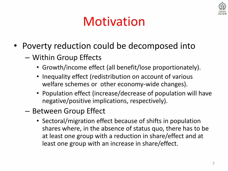
• Poverty reduction could be decomposed into – Within Group Effects

• Growth/income effect (all benefit/lose proportionately).

• Inequality effect (redistribution on account of various welfare schemes or other economy-wide changes).

• Population effect (increase/decrease of population will have negative/positive implications, respectively).

– Between Group Effect • Sectoral/migration effect because of shifts in population

shares where, in the absence of status quo, there has to be at least one group with a reduction in share/effect and at least one group with an increase in share/effect.

3

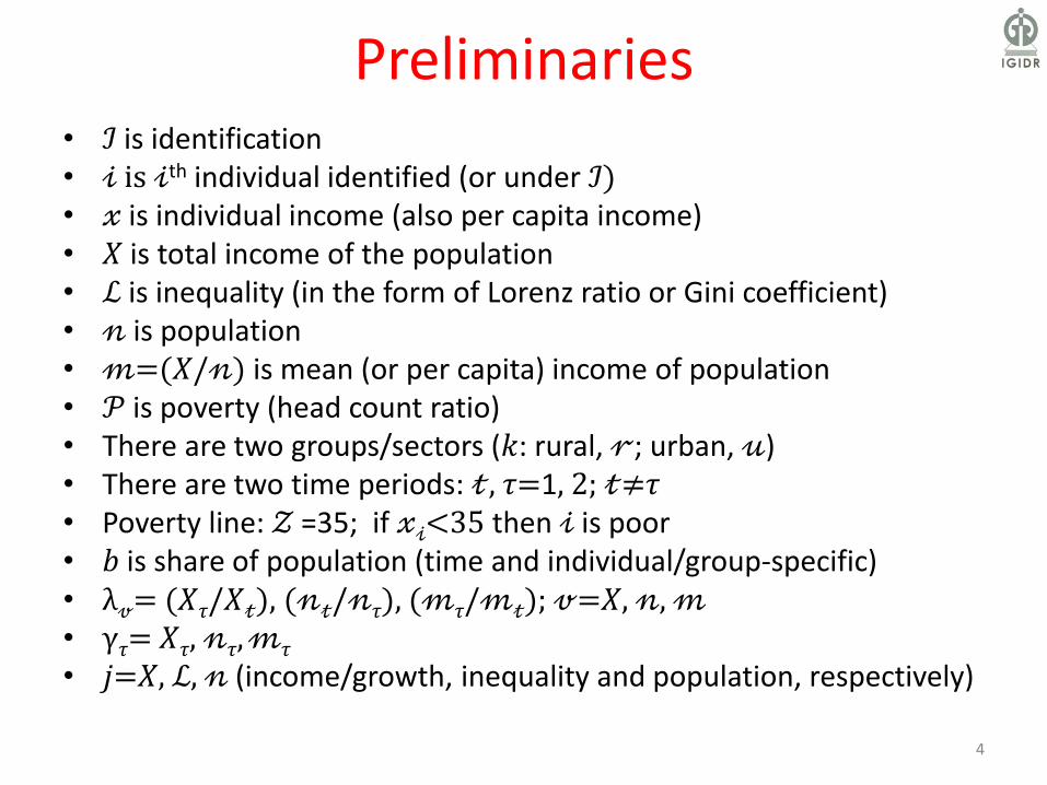
Preliminaries • ℐ is identification • 𝒾 is 𝒾th individual identified (or under ℐ) • 𝓍 is individual income (also per capita income) • 𝑋 is total income of the population • ℒ is inequality (in the form of Lorenz ratio or Gini coefficient) • 𝓃 is population • 𝓂=(𝑋/𝓃) is mean (or per capita) income of population • 𝒫 is poverty (head count ratio) • There are two groups/sectors (𝑘: rural, 𝓇; urban, 𝓊) • There are two time periods: 𝓉, 𝜏=1, 2; 𝓉≠𝜏 • Poverty line: 𝒵 =35; if 𝓍𝒾<35 then 𝒾 is poor • 𝑏 is share of population (time and individual/group-specific) • λ𝓋= (𝑋𝜏/𝑋𝓉), (𝓃𝓉/𝓃𝜏), (𝓂𝜏/𝓂𝓉); 𝓋=𝑋, 𝓃, 𝓂 • γ𝜏= 𝑋𝜏, 𝓃𝜏, 𝓂𝜏

• 𝑗=𝑋, ℒ, 𝓃 (income/growth, inequality and population, respectively)

4

Counting Poor

• In the next two slides, we will give examples of counting poor for two periods.

• One could consider the examples as sample observations or even actual population at two different time periods.

• One could also consider the two examples as two situations/locations, but we will keep that aside for the time being.

5

Counting Poor, Period 1

ℐ1 𝓍1 𝒫1

Su 10 1

Ma 20 1

El 30 1

Ki 40 0

𝓃1=4 25 3/4

6

.

Counting Poor, Period 2

7

.

ℐ2 𝓍2 𝒫2

Bh 20 1

Tu 30 1

Ka 40 0

Li 50 0

Ch 60 0

𝓃2=5 30 2/5

Change in Poverty

𝒫2-𝒫1 =(2/5)-(3/4)

=40%-75%

=-35%

Using the previous two slides, total poverty change is

8

Decomposing Poverty Change

• Poverty change can be decomposed to within- and between-group effects.

• Within-group has three broad effects: growth, inequality and population.

• The within-group effects will depend on the base period (we use period 2 as base).

• Given base, there will be six possible ways to compute three within-group effects (depends on sequence of each).

9

Six possible Sequences

10

• Growth-Inequality-Population • Growth-Population-Inequality • Inequality-Growth-Population • Inequality-Population-Growth • Population-Growth-Inequality • Population-Inequality-Growth

These six possible sequences have 12 possible specific attributions.

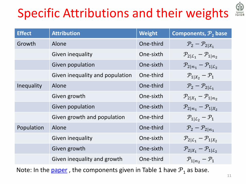
Specific Attributions and their weights

Effect Attribution Weight Components, 𝒫2 base

Growth Alone One-third 𝒫2 − 𝒫2|𝑋1

Given inequality One-sixth 𝒫2|ℒ1 − 𝒫1|𝓃2

Given population One-sixth 𝒫2|𝓃1 − 𝒫1|ℒ2

Given inequality and population One-third 𝒫1|𝑋2 − 𝒫1

Inequality Alone One-third 𝒫2 − 𝒫2|ℒ1

Given growth One-sixth 𝒫2|𝑋1 − 𝒫1|𝓃2

Given population One-sixth 𝒫2|𝓃1 − 𝒫1|𝑋2

Given growth and population One-third 𝒫1|ℒ2 − 𝒫1

Population Alone One-third 𝒫2 − 𝒫2|𝓃1

Given inequality One-sixth 𝒫2|ℒ1 − 𝒫1|𝑋2

Given growth One-sixth 𝒫2|𝑋1 − 𝒫1|ℒ2

Given inequality and growth One-third 𝒫1|𝓃2 − 𝒫1

11 Note: In the paper , the components given in Table 1 have 𝒫1 as base.

Counting poor with conditions

𝒫1 Poverty in period 1

𝒫1|𝑋2 Poverty in period 1 with income of period 2

𝒫1|ℒ2 Poverty in period 1 with inequality of period 2

𝒫1|𝓃2 Poverty in period 1 with population of period 2

𝒫2 Poverty in period 2

𝒫2|𝑋1 Poverty in period 2 with income of period 1

𝒫2|ℒ1 Poverty in period 2 with inequality of period 1

𝒫2|𝓃1 Poverty in period 2 with population of period 1

12

To obtain the 12 components indicated in the previous slide, we need the following:

Note: 𝒫1|ℒ2= 𝒫2|𝓂1 ; 𝒫2|ℒ1= 𝒫1|𝓂2 (see proposition 4 in paper).

Controlling growth and population

• For growth effect, one imposes the total income of the other period by increasing each individual’s income proportionately (by the same growth rate).

• For population, a proportionate change can be interpreted as a change in the multiplier or adult equivalence scale that each observation represents.

13

Note on controlling inequality

• For controlling inequality, one has to ensure that shares of population and shares of income are that of the other period. We do this by using the observation of the other period with total income and total population of the current period.

14

Computing Poverty with Conditions

15

𝒫𝓉|γ𝜏 = 𝑏𝑖𝓉𝑧 − λ𝑣𝑥𝑖𝓉𝑧

𝑛𝓉

𝑖𝓉=1

λ𝓋= (𝑋𝜏/𝑋𝓉), (𝓃𝓉/𝓃𝜏), (𝓂𝜏/𝓂𝓉) γ𝜏= 𝑋𝜏, 𝓃𝜏, 𝓂𝜏

Counting poor with conditions, period 1

ℐ1 𝓍1 𝒫1 𝓍1|𝑋2 𝒫1|𝑋2 𝓍1|𝓃2 𝒫1|𝓃2 𝓍1|𝓂2 𝒫1|𝓂2

Su 10 1 20 1 8 1 16 1

Ma 20 1 40 0 16 1 32 1

El 30 1 60 0 24 1 48 0

Ki 40 0 80 0 32 1 64 0

𝓃1 25 3/4 50 1/4 20 1 40 1/2

Total 100 75% 200 25% 100 100% 200 50%

16

.

Note: 𝓍1|𝓂2 = 𝓍2|ℒ1; 𝒫1|𝓂2 = 𝒫2|ℒ1 (see proposition 4 in paper).

Counting poor with conditions, period 2

ℐ2 𝓍2 𝒫2 𝓍2|𝑋1 𝒫2|𝑋1 𝓍2|𝓃1 𝒫2|𝓃1 𝓍2|𝓂1 𝒫2|𝓂1

Bh 20 1 10 1 25.0 1 12.50 1

Tu 30 1 15 1 37.5 0 18.75 1

Ka 40 0 20 1 50.0 0 25.00 1

Li 50 0 25 1 62.5 0 31.25 1

Ch 60 0 30 1 75.0 0 37.50 0

𝓃2 40 2/5 20 1 50.0 1/5 25.00 4/5

Total 200 40% 100 100% 200 20% 100 80%

17

.

Note: 𝓍2|𝓂1 = 𝓍1|ℒ2; 𝒫2|𝓂1= 𝒫1|ℒ2 (see proposition 4 in paper).

Attribution-specific Effects Effect Attribution Weight Components, 𝒫2 base

Growth Alone One-third 𝒫2 − 𝒫2|𝑋1 -1/5 -11/20

Given inequality One-sixth 𝒫2|ℒ1 − 𝒫1|𝓃2 -1/12

Given population One-sixth 𝒫2|𝓃1 − 𝒫1|ℒ2 -1/10

Given inequality and population One-third 𝒫1|𝑋2 − 𝒫1 -1/6

Inequality Alone One-third 𝒫2 − 𝒫2|ℒ1 -1/30 -1/40

Given growth One-sixth 𝒫2|𝑋1 − 𝒫1|𝓃2 0

Given population One-sixth 𝒫2|𝓃1 − 𝒫1|𝑋2 -1/120

Given growth and population One-third 𝒫1|ℒ2 − 𝒫1 1/60

Population Alone One-third 𝒫2 − 𝒫2|𝓃1 1/15 9/40

Given inequality One-sixth 𝒫2|ℒ1 − 𝒫1|𝑋2 1/24

Given growth One-sixth 𝒫2|𝑋1 − 𝒫1|ℒ2 1/30

Given inequality and growth One-third 𝒫1|𝓃2 − 𝒫1 1/12

Total (Growth + Ineq + Popn) 𝒫2 − 𝒫1 -7/20

18

Note: In the paper , the components given in Table 1 have 𝒫1 as base. The values given in column 5 are after applying weights of column 3.

Bringing Subgroups – rural and urban

• Now, we bring in groups – rural and urban.

• In period 1: Su, Ma and El are rural; Ki is urban.

• In period 2: Bh, and Tu are rural; Ka, Li and Ch are urban.

• We now count poor with conditions for the rural and urban subgroups.

19

Counting poor: sector-specific, period 1

ℐ1 𝓍1 𝒫1 𝓍1|𝑋2 𝒫1|𝑋2 𝓍1|𝓃2 𝒫1|𝓃2 𝓍2|ℒ1 𝒫2|ℒ1

Su 10 1 13.3 1 15 1 20 1

Ma 20 1 26.7 1 30 1 40 0

El 30 1 40.0 0 45 0 60 0

𝓃1𝓇 20 1 26.7 2/3 30 2/3 40 1/3

Tot1𝓇 60 100% 80 67% 60 67% 80 33%

Ki 40 0 120 0 13.3 1 35 0

𝓃1𝓊 40 0 120 0 13.3 1 35 0

Tot1𝓊 40 0% 120 0% 40 100% 105 0%

𝓃1* 25 3/4 50 1/2 20 13/15 30 2/15

Tot1* 100 75% 200 50% 100 87% 150 13%

20

.

Note: * weighted averages.

Counting poor: sector-specific, period 2 ℐ2 𝓍2 𝒫2 𝓍2|𝑋1 𝒫2|𝑋1 𝓍2|𝓃1 𝒫2|𝓃1 𝓍1|ℒ2 𝒫1|ℒ2

Bh 30 1 22.5 1 20.0 1 15 1

Tu 50 0 37.5 0 33.3 1 25 1

𝓃2𝓇 40 1/2 30 1/2 26.7 1 20.0 1

Tot2𝓇 80 50% 60 50% 80 100% 60 100%

Ka 20 1 6.7 1 60 0 20 1

Li 40 0 13.3 1 120 0 40 0

Ch 60 0 20.0 1 180 0 60 0

𝓃2𝓊 40 1/3 13.3 1 180 0 40 1/3

Tot2𝓊 120 33.3% 40 100% 120 0% 40 33%

𝓃2* 40 2/5 20 4/5 50 3/4 25 5/6

Tot2* 200 40% 100 80% 200 75% 100 83% 21

.

Note: * weighted averages.

Attributions: sector-specific Effect Attribution Weight Rural Urban Combined

Growth Alone One-third 0 -2/9 -2/15

Given inequality One-sixth -1/18 -1/6 -11/90

Given population One-sixth 0 -1/18 -1/72

Given inequality and population One-third -1/9 0 -1/12

Inequality Alone One-third 1/18 1/9 4/45

Given growth One-sixth -1/36 0 -1/90

Given population One-sixth 1/18 0 1/24

Given growth and population One-third 0 1/9 1/36

Population Alone One-third -1/6 1/9 -7/60

Given inequality One-sixth -1/18 0 -11/180

Given growth One-sixth -1/12 1/9 -1/180

Given inequality and growth One-third -1/9 1/3 7/180

22

Note: The values given in columns 4-6 are based on slides 20 and 21 after applying weights indicated in column 3.

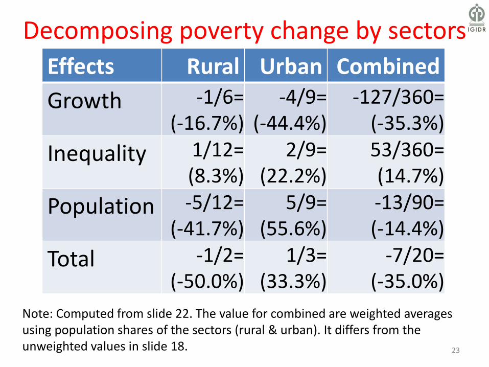
Decomposing poverty change by sectors

Effects Rural Urban Combined

Growth -1/6= (-16.7%)

-4/9= (-44.4%)

-127/360= (-35.3%)

Inequality 1/12= (8.3%)

2/9= (22.2%)

53/360= (14.7%)

Population -5/12= (-41.7%)

5/9= (55.6%)

-13/90= (-14.4%)

Total -1/2= (-50.0%)

1/3= (33.3%)

-7/20= (-35.0%)

23

Note: Computed from slide 22. The value for combined are weighted averages using population shares of the sectors (rural & urban). It differs from the unweighted values in slide 18.

Combining within- & between-groups

24

• Average of the group-specific population shares for the two periods multiplied by attribution-specific poverty change will give the within-group effects.

• Average of the group-specific poverty values for the two periods multiplied by group-specific change in population shares will give the between-group effect.

Within- and between-group effects: formula

25

∆𝒫 = 𝑏𝑘1 + 𝑏𝑘22𝑘=𝓇,𝓊

∆𝒫𝑗𝑘𝑗

+ 𝒫𝑘1 +𝒫𝑘22

∆𝑏𝑘𝑘=𝓇,𝓊

; 𝑗 = 𝑋, ℒ,𝓃

Within- and between-group effects: result (preliminary)

26

Effect Attribution Rural Urban Combin-ed (𝓇+𝓊)

Within Growth 2340∗−16 17

40∗−49 −41

144

Inequality 2340∗112

1740∗29

41288

Population 2340∗−512

1740∗59

−1288

Total within −2380 17

120 −748

Between Sectoral shift 34∗−720

16∗720

−49240

Total (within + between) −1120 1

5 −720

Within- and between-group effects: result (per cent)

27

Effect Attribution Rural Urban Combined (𝓇 + 𝓊)

Within Growth -9.6% -18.9% -28.5%

Inequality 4.8% 9.4% 14.2%

Population -24.0% 23.6% -0.3%

Total within -28.8% 14.2% -14.6%

Between Sectoral shift -26.3% 5.8% -20.4%

Total (within + between) -55.0% 20.0% -35.0%

Within- and between-group effects: result for India (2004-05 and 2009-10)

28

Effect Attribution Rural Urban Combined (𝓇 + 𝓊)

Within Growth -9.45% -4.32% -13.77%

Inequality -0.40% 0.53% 0.13%

Population 4.13% 2.39% 6.51%

Total within -5.72% -1.41% -7.13%

Between Sectoral shift -0.63% 0.39% -0.25%

Total (within + between) -6.35% -1.02% -7.37% Note: Table 4 of the paper.

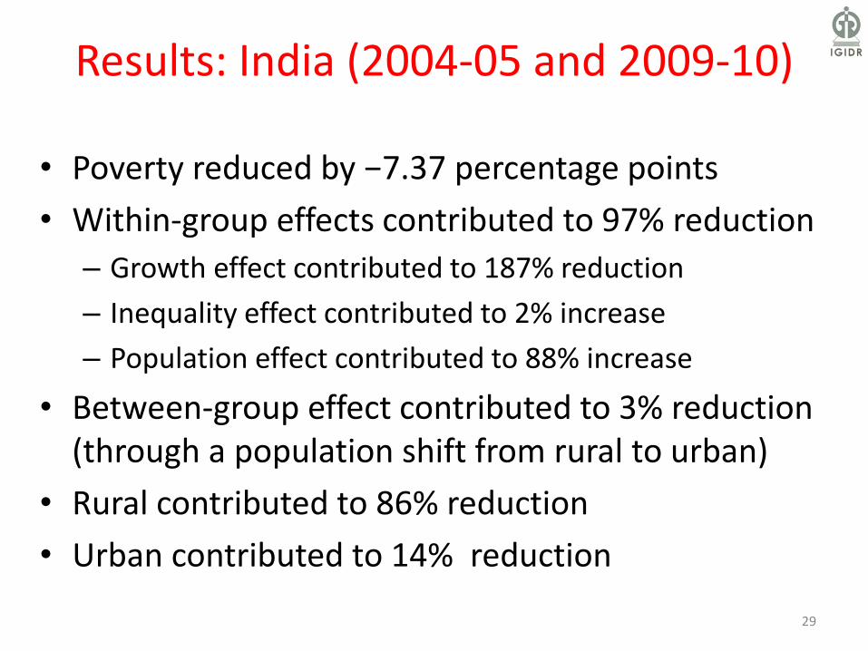
Results: India (2004-05 and 2009-10)

29

• Poverty reduced by −7.37 percentage points

• Within-group effects contributed to 97% reduction

– Growth effect contributed to 187% reduction

– Inequality effect contributed to 2% increase

– Population effect contributed to 88% increase

• Between-group effect contributed to 3% reduction (through a population shift from rural to urban)

• Rural contributed to 86% reduction

• Urban contributed to 14% reduction

30

For a detailed discussion see the paper

Decomposing Poverty Change: Deciphering Change in Total Population and Beyond, Review of Income and Wealth (available under open access).

See related blog, Growth, Inequality and Population Effects on Poverty Reduction

I thank Ram Nidhish and Durgesh C Pathak for their comments on an earlier version.