decomposing the luenberger-hicks-moorsteen total …

DECOMPOSING THE LUENBERGER-HICKS-MOORSTEEN

TOTAL FACTOR PRODUCTIVITY INDICATOR: AN

APPLICATION TO U.S. AGRICULTURE

FREDERIC ANG AND PIETER JAN KERSTENS

Abstract. This paper introduces a decomposition of the additively completeLuenberger-Hicks-Moorsteen Total Factor Productivity indicator into the usualcomponents: technical change, technical inefficiency change and scale ineffi-ciency change. Our approach is general in that it does not require differen-tiability or convexity of the production technology. Using a nonparametricframework, the empirical application focuses on the agricultural sector at thestate-level in the U.S. over the period 1960 − 2004. The results show thatLuenberger-Hicks-Moorsteen productivity increased substantially in the consi-dered period. This productivity growth is due to output growth rather thaninput decline, although the extent depends on the convexity assumption of thetechnology. Technical change is the main driver, while the role of technical in-efficiency change and scale inefficiency change also depends on the convexityassumption of the technology.Keywords Data Envelopment Analysis, Luenberger-Hicks-Moorsteen total fac-tor productivity indicator, decomposition, non-convex technology, additive com-pletenessJEL codes C43, D24, Q10

Department of Economics, Swedish University of Agricultural Sciences, Box7013, SE-750 07 Uppsala, Sweden

Center for Economic Studies, KU Leuven, E. Sabbelaan 53, B-8500 Kortrijk,Belgium, tel: +3216330765

The authors gratefully acknowledge two anonymous referees for their valuable comments andsuggestions. The authors also thank Laurens Cherchye for helpful comments and suggestions.Email [email protected] for correspondence. Both authors have contributed equallyto this paper. Any remaining errors are the responsibility of the authors.

1

2 F. ANG AND P. J. KERSTENS

1. Introduction

Assessing the drivers of productivity growth is important for business and eco-nomic policy. Their identification allows monitoring of industries and can guidepolicymakers in their decisions. Hence, an abundant literature has sought to de-compose various measures of productivity growth into components of technicalchange, efficiency change and scale efficiency change.1 The literature has largelyfocused on ratio-based productivity “indexes”. Yet, O’Donnell (2012a) recentlyshows that not all such decomposable indexes are “multiplicatively complete” (i.e.consisting of a ratio of an output aggregator to an input aggregator), while allmultiplicatively complete indexes are decomposable in this way. He demonstratesthat the class of multiplicatively complete productivity indexes includes Laspey-res, Paasche, Fischer, Tornqvist and Bjurek (1996)’s Hicks-Moorsteen indexes, butdoes not include the popular Malmquist index of Caves et al. (1982).Ratio-based productivity indexes are undefined when one or more of the vari-

ables are equal or close to zero (Balk et al., 2003). Difference-based productivity“indicators” do not suffer from this problem and are thus particularly useful inregulatory contexts.Difference-based indicators were developed to measure Total Factor Productivity

(TFP) growth based on Luenberger (1992)’s shortage function. This directionaldistance function, introduced by Chambers et al. (1996) in a production context,extends the Shephard input and output distance functions by allowing for simulta-neous contraction of inputs and expansion of outputs. Chambers (2002) introduceda general difference-based Luenberger productivity indicator which can be decom-posed in a technical change and efficiency change component (Chambers et al.,1996).2 Since its introduction, it has frequently been applied in empirical ap-plications (e.g. Nakano and Managi (2008)) and additional decompositions of itstechnical change component (e.g. Briec and Peypoch (2007)) and efficiency changecomponent (e.g. Epure et al. (2011)) have been proposed in the literature. Howe-ver, the Luenberger productivity indicator is not “additively complete” (i.e. con-sisting of a difference between an output aggregator and an input aggregator) andthus cannot be disentangled into components of output growth and input growth.Briec and Kerstens (2004) introduced the Luenberger-Hicks-Moorsteen (LHM)

TFP indicator, which is a difference-based, additively complete alternative to the

1See Fare et al. (1998) and Grosskopf (2003) for historical overviews.2The “economic” approach to productivity measurement requires price information and if

in addition (i) some assumptions can be made about firm behavior and (ii) the technology isapproximated by a known flexible functional form up to the second order, then one can use a“superlative” index as advocated by Diewert (1976). Chambers (2002) showed that the Bennet-Bowley indicators are exact and superlative approximations of the Luenberger productivity in-dicator under (i) profit-maximizing behavior and (ii) a quadratic technology directional distancefunction. A corresponding superlative indicator for the LHM TFP indicator is currently notknown.

DECOMPOSING THE LHM TFP INDICATOR 3

ratio-based, multiplicatively complete Hicks-Moorsteen index.3 Notwithstandingthe attractive properties of the LHM TFP indicator, only few empirical studiescan be found in the literature (e.g. Barros et al. (2008) and Managi (2010)). Onepossible reason for the limited number of applications is the fact that a full de-composition into components of technical change, technical inefficiency change andscale inefficiency change has hitherto not been developed. A first effort was madeby Managi (2010) who decomposed the LHM TFP indicator into components oftechnical change and (in)efficiency change. However, this decomposition lacksa scale inefficiency change component and does not correctly capture technicalchange and technical inefficiency change (see Appendix A). No full decompositionof a difference-based TFP indicator being additively complete is thus presentlyknown in the literature.The current paper contributes to the existing literature by introducing a de-

composition of the additively complete LHM TFP indicator into components oftechnical change, technical inefficiency change and scale inefficiency change. Ourdecomposition is general in that it does not require convexity or differentiability ofthe technology set. It is similar to Diewert and Fox (2014, 2017)’s decompositionof the ratio-based Hicks-Moorsteen TFP index.Using a nonparametric framework, we illustrate the decomposition with an em-

pirical application to state-level data of the U.S. agricultural sector over the period1960− 2004. Since our decomposition is suitable for non-convex as well as convextechnologies, we demonstrate its flexibility by using the Free Disposal Hull as wellas Data Envelopment Analysis. To the best of our knowledge, no other studiesusing the same dataset have investigated the issue of potential non-convexities.However, we believe that such an investigation is particularly relevant in the con-text of the agricultural sector. Inputs such as capital equipment are nondivisible,potentially leading to non-convexities.This paper is structured as follows. The next section describes Luenberger’s

directional distance function and the LHM TFP indicator. We then introduce ourcomplete decomposition and apply this to state-level data of the U.S. agriculturalsector over the period 1960− 2004. The final section concludes.

2. The Luenberger-Hicks-Moorsteen TFP indicator

Let xt ∈ Rn+ be the nonnegative inputs that are used to produce nonnegative

outputs yt ∈ Rm+ . We define the technology set in the usual way:

Y t ={

(xt,yt) ∈ Rn+m+ |xt can produce yt

}

.

Furthermore, we make the following minimal assumptions on the technology set(Chambers, 2002):

3See Briec et al. (2012) for exact relations between the Luenberger-Hicks-Moorsteen TFPindicator and the Hicks-Moorsteen TFP index.


Axiom 1 (Closedness). Y t is closed.

Axiom 2 (Free disposability of inputs and outputs). if (x′t,−y′

t) ≥ (xt,−yt) then(xt,yt) ∈ Y t ⇒ (x′

t,x′t) ∈ Y t.

Axiom 3 (Inaction). Inaction is possible: (0n,0m) ∈ Y t.

Convexity of the technology set is thus not a necessary condition for our decom-position.4 We illustrate this in our empirical application.Luenberger’s directional distance function is a measure of technical inefficiency

as it simultaneously contracts inputs and expands outputs. The directional dis-tance function proposed by Chambers et al. (1996) is:

(1) Dt(xt,yt;gt) = sup{

β ∈ R : (xt − βgit,yt + βgo

t ) ∈ Y t

}

,

if (xt − βgit,yt + βgo

t ) ∈ Y t for some β and Dt(xt,yt;gt) = −∞ otherwise. Here,gt = (gi

t,got ) represents the direction vector. The directional distance function is

a special case of Luenberger (1992)’s shortage function.We denote the time-related directional distance function for (a, b) ∈ {t, t+ 1}×

{t, t+ 1}:

Db(xa,ya;ga) = sup{

β ∈ R : (xa − βgia,ya + βgo

a) ∈ Yb

}

.

Next, we turn to the Luenberger-Hicks-Moorsteen (LHM) TFP indicator pro-posed by Briec and Kerstens (2004). This can be seen as the difference-basedequivalent of the ratio-based Hicks-Moorsteen (HM) TFP index. They define theLHM TFP indicator with base period t as the difference between a Luenbergeroutput quantity indicator and a Luenberger input quantity indicator:

LHMt(xt+1,yt+1,xt,yt;gt,gt+1)(2)

=[

Dt(xt,yt; (0,got ))−Dt(xt,yt+1; (0,g

ot+1))

]

−[

Dt(xt+1,yt; (git+1, 0))−Dt(xt,yt; (g

it, 0))

]

≡ LOt(xt,yt,yt+1;got ,g

ot+1)− LIt(xt,xt+1,yt;g

it,g

it+1).

Similarly, a base period t+ 1 LHM TFP indicator is defined as:

LHMt+1(xt+1,yt+1,xt,yt;gt,gt+1)(3)

=[

Dt+1(xt+1,yt; (0,got ))−Dt+1(xt+1,yt+1; (0,g

ot+1))

]

−[

Dt+1(xt+1,yt+1; (git+1, 0))−Dt+1(xt,yt+1; (g

it, 0))

]

≡ LOt+1(xt+1,yt+1,yt;got ,g

ot+1)− LIt+1(xt,xt+1,yt+1;g

it,g

it+1).

4In fact, the LHM TFP indicator and our decomposition are applicable to a wider rangeof non-convex models that satisfy the above axioms and for which the directional distancefunction can be defined. Examples of these non-convex models include the Constant-Elasticity-of-Substitution-Constant-Elasticity-of-Transformation model of Fare et al. (1988), relaxed con-vexity model of Petersen (1990) and Bogetoft (1996), selective convexity model of Podinovski(2005) and B-convexity model of Briec and Liang (2011).


O’Donnell (2012a) (p.258, footnote 5) defines additive completeness as follows:

Definition 1 (Additive completeness). Formally, let TFPI(xt, qt, xs, qs) denote

an index number that compares TFP in period s with TFP in period t using period

s as a base. TFPI(xt, qt, xs, qs) is additively complete if and only if it can be

expressed in the form TFPI(xt, qt, xs, qs) = Q(qt)−Q(qs)−X(xt) +X(xs) whereQ(·) and X(·) are non-negative non-decreasing functions satisfying the translation

property Q(q + λq) = Q(q) + λ and X(x+ λx) = X(x) + λ for λ > 0.

LHMt(·) and LHMt+1(·) are “additively complete” in O’Donnell’s sense. Thiscan be verified from their definitions above where the directional distance function,along with its corresponding direction vector, serves as the output (using (0,go

s))and input (using (gi

s, 0)) aggregator functions.5

Finally, one takes an arithmetic average of LHMt and LHMt+1 to avoid anarbitrary choice of base periods:6

LHMt,t+1(xt,yt,xt+1,yt+1;gt,gt+1) =1

2[LHMt + LHMt+1] .(4)

The HM TFP index is defined as the ratio of an output index to an input index.Similarly, we can show that the LHM TFP indicator equals the difference bet-ween an output indicator and an input indicator, which are themselves arithmeticaverages of two output and two input indicators:

LHMt,t+1 =1

2[LOt + LOt+1]−

1

2[LIt + LIt+1](5)

≡ LOt,t+1 − LIt,t+1.

5Luenberger (1992)’s shortage function differs from Chambers (2002)’ Luenberger productivityindicator. The shortage function satisfies the translation property. It is an aggregator functionthat can be used to compute components of an additively complete indicator (such as the LHMTFP indicator), but is not additively complete. Chambers (2002) defines the Luenberger pro-ductivity indicator as follows:

Lt,t+1(xt,yt,xt+1,yt+1;gt,gt+1)

=1

2

[

(Dt(xt,yt;gt)−Dt(xt+1,yt+1;gt+1))

+ (Dt+1(xt,yt;gt)−Dt+1(xt+1,yt+1;gt+1))]

,

All directional vectors are determined in the input direction as well as the output direction, i.e.ga = (gi

a,goa) > 0. This prevents us from disentangling the indicator into separate output and

input aggregator functions.6This average can be harder to interpret in regulatory and managerial contexts in which a

clearer target is required. This can easily be accounted for by a different choice of weights forboth periods: i.e. we can define LHMt,t+1 = ζLHMt + (1− ζ)LHMt+1 with weights ζ ∈ [0, 1].One can then for example set ζ = 0 or ζ = 1. These weights trickle down in the technical changeand scale inefficiency change components of our decomposition in a straightforward way.


3. Decomposition of the Luenberger-Hicks-Moorsteen indicator

This section introduces our LHM decomposition along with illustrative figuresin the one input - one output dimension to provide the intuition. We show anexample with a non-convex technology (i.e. Free Disposal Hull), as convexity isnot a necessary assumption for our decomposition. Note, however, that one canalso use our approach for a convex technology.In line with the decomposition of the HM TFP index, the LHM TFP indicator

can be decomposed using the output direction or input direction.7 We focus onthe decomposition using the output direction, but provide a similar decompositionusing the input direction in Appendix B. Our LHM decomposition is a specificcase (analogous to the multiplicatively complete case discussed in Section 3.7 ofO’Donnell (2012a)) of an additively complete indicator that uses the directionaldistance function as the aggregator function for both inputs and outputs. Hence,in our case the mix efficiency change components are all 0 and our decompositionconsists of three components:

(6) LHMt,t+1 = ∆T ot,t+1 +∆TEIot,t+1 +∆SECo

t,t+1,

representing technical change, technical inefficiency change and scale inefficiencychange respectively.8 Given the close relation to the HM TFP index, it is nosurprise that our decomposition is similar to Diewert and Fox (2014, 2017)’s de-composition of the HM TFP index.The technical change component is

∆T ot,t+1 =

1

2{[Dt+1(xt,yt; (0,g

ot ))−Dt(xt,yt; (0,g

ot ))](7)

+[

Dt+1(xt+1,yt+1; (0,got+1))−Dt(xt+1,yt+1; (0,g

ot+1))

]}

≡1

2

{

∆T ot +∆T o

t+1

}

.

Technical change ∆T ot,t+1 is the arithmetic average of ∆T o

t and ∆T ot+1. Figure 1

depicts these technical change components. The arithmetic average is used to avoidan arbitrary choice of the observation under evaluation. Here, ∆T o

t measures thedifference in efficiency for observation (xt,yt) evaluated against production frontiert + 1 and t. An upward (downward) shift of the production frontier between tand t + 1, indicating technical progress (regress), results in a positive (negative)

7The technical change and technical inefficiency change components in particular are comple-tely determined by this choice. The additive completeness property of the LHM TFP indicatorcan guide this decision by checking whether LHM TFP is mostly driven by LOt,t+1 or LIt,t+1.This contrasts with the Luenberger productivity indicator where both inputs and outputs con-tribute to its components.

8Managi (2010)’s decomposition lacks a scale inefficiency change component. We refer toAppendix A for a discussion.


difference. ∆T ot+1 is similar to ∆T o

t but evaluated for observation (xt+1,yt+1).Thus, technical change measures (local) shifts of the production frontier itself.

t+ 1

t

b

b

∆T ot+1

∆T ot

(xt,yt)

(xt+1,yt+1)

x

y

Figure 1. Technical change

The technical inefficiency change component is

∆TEIot,t+1 = Dt(xt,yt; (0,got ))−Dt+1(xt+1,yt+1; (0,g

ot+1)),(8)

and measures the change between period t and period t+1 in the relative position tothe production frontier. Positive (negative) values of ∆TEIot,t+1 indicate efficiencyimprovement (deterioration) over time: (xt+1,yt+1) is located closer (farther) tothe t + 1 frontier than (xt,yt) was to the t frontier. In Figure 2 this means thatDt+1(xt+1,yt+1) is smaller (larger) than Dt(xt,yt). Note that ∆TEIo only mea-sures the evolution in technical efficiency of the observation under considerationwithout taking into account changes of the production frontier over time.This technical inefficiency change component can be further decomposed in the

same way as done by Epure et al. (2011) for the Luenberger indicator into “pure”inefficiency and, for example, congestion changes.


t+ 1

t

b

b

Dt+1(·)

Dt(·)

(xt,yt)

(xt+1,yt+1)

x

y

Figure 2. Technical inefficiency change

Finally, from the residual

LHMt,t+1−∆T ot,t+1 −∆TEIot,t+1(9)

=1

2

{[

Dt(xt+1,yt+1; (0,got+1))−Dt(xt,yt+1; (0,g

ot+1))

]

+ [Dt+1(xt+1,yt; (0,got ))−Dt+1(xt,yt; (0,g

ot ))]}

−1

2

{[


it, 0))

]

+[


it, 0))

]}

,

we can distill the scale inefficiency change component as follows. First, we definethe projections of yt and yt+1 on the production frontier at time t using notationof Diewert and Fox (2017):

y∗t = yt +Dt(xt,yt; (0,g

ot ))g

ot(10a)

y∗∗t+1 = yt+1 +Dt(xt+1,yt+1; (0,g

ot+1))g

ot+1(10b)

Similarly, we define the projections of yt and yt+1 on the production frontier attime t+ 1:

y∗∗t = yt +Dt+1(xt,yt; (0,g

ot ))g

ot(11a)

y∗t+1 = yt+1 +Dt+1(xt+1,yt+1; (0,g

ot+1))g

ot+1(11b)


Then, respectively adding and subtractingDt(xt,yt; (0,got )) andDt+1(xt+1,yt+1; (0,g

ot+1))

to and from (9), and using the translation property of the directional distancefunction and the definitions of the projections above, we find the scale inefficiencychange component:

∆SECot,t+1 =

1

2

{[

Dt(xt,y∗t ; (0,g

ot ))−Dt(xt,y

∗∗t+1; (0,g

ot+1))

]

(12)

−[


it, 0))

]

+[

Dt+1(xt+1,y∗∗t ; (0,go

t ))−Dt+1(xt+1,y∗t+1; (0,g

ot+1))

]

−[


it, 0))

]}

≡1

2

{

SOCot − SICo

t + SOCot+1 − SICo

t+1

}

≡1

2

{

∆SECot +∆SECo

t+1

}

,

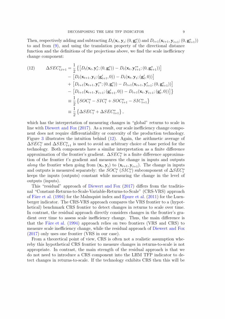
which has the interpretation of measuring changes in “global” returns to scale inline with Diewert and Fox (2017). As a result, our scale inefficiency change compo-nent does not require differentiability or convexity of the production technology.Figure 3 illustrates the intuition behind (12). Again, the arithmetic average of∆SECo

t and ∆SECot+1 is used to avoid an arbitrary choice of base period for the

technology. Both components have a similar interpretation as a finite differenceapproximation of the frontier’s gradient. ∆SECo

t is a finite difference approxima-tion of the frontier t’s gradient and measures the change in inputs and outputsalong the frontier when going from (xt,yt) to (xt+1,yt+1). The change in inputsand outputs is measured separately: the SOCo

t (SICot ) subcomponent of ∆SECo

t

keeps the inputs (outputs) constant while measuring the change in the level ofoutputs (inputs).This “residual” approach of Diewert and Fox (2017) differs from the traditio-

nal “Constant-Returns-to-Scale-Variable-Returns-to-Scale” (CRS-VRS) approachof Fare et al. (1994) for the Malmquist index and Epure et al. (2011) for the Luen-berger indicator. The CRS-VRS approach compares the VRS frontier to a (hypot-hetical) benchmark CRS frontier to detect changes in returns to scale over time.In contrast, the residual approach directly considers changes in the frontier’s gra-dient over time to assess scale inefficiency change. Thus, the main difference isthat the Fare et al. (1994) approach relies on two frontiers (VRS and CRS) tomeasure scale inefficiency change, while the residual approach of Diewert and Fox(2017) only uses one frontier (VRS in our case).From a theoretical point of view, CRS is often not a realistic assumption whe-

reby this hypothetical CRS frontier to measure changes in returns-to-scale is notappropriate. In contrast, the main strength of the residual approach is that wedo not need to introduce a CRS component into the LHM TFP indicator to de-tect changes in returns-to-scale. If the technology exhibits CRS then this will be


t+ 1

t

bb

b b

b

b

b

b

SOCot+1

SOCot

SICot+1

SICot(xt,yt) (xt+1,yt)

(xt,yt+1) (xt+1,yt+1)

(xt,y∗

t )

(xt,y∗∗

t+1)

(xt+1,y∗∗

t )

(xt+1,y∗

t+1)

x

y

Figure 3. Scale inefficiency change

automatically reflected in zero values for the ∆SECot,t+1 component even if we

use a VRS approximation. Of course, depending on the application at hand andresults of a preliminary test on returns-to-scale, the LHM TFP indicator and ourdecomposition can also be computed under other returns-to-scale assumptions.From a practical point of view, an obvious drawback to the “CRS-VRS” approachis that it is sensitive to outliers, because the CRS frontier can be spanned by afew (extreme) observations. This drawback can be reduced by using appropriatetechniques such as order-m (Cazals et al., 2002) or order-α (Aragon et al., 2005).The accuracy of the residual approach to approximate the gradient of the frontier

depends on the “step-size”, i.e. the gap SICot and SICo

t+1 between the frontierprojections of xt and xt+1 for the decomposition using output directions. Thelarger the step-size, the cruder the approximation.9 Thus, a big change in inputsfor a DMU from period t to period t + 1 can give a cruder approximation of thefrontier’s gradient.As a final remark, observe that both ∆T o

t,t+1 and ∆SECot,t+1 are the arithmetic

average of a Laspeyres (using base period t) and a Paasche (using base periodt+ 1) type indicator.

9This step-size is analogous to h in the commonly used definition of a derivative of a function

f : f ′(x) = limh→0f(x+h)−f(x)

h. The more h approaches zero, the better the approximation of

the derivative at the evaluated point. Likewise, the smaller SICot and SICo

t+1, the better the

approximation of the frontier’s gradient.


4. Empirical application: U.S. agriculture

We investigate LHM TFP growth of U.S. agriculture across 48 states10. Weuse our newly developed LHM decomposition to determine the main drivers ofproductivity growth. Specifically, we investigate the extent to which LHM TFPgrowth is driven by output growth and input growth, on the one hand, and techni-cal change, technical inefficiency change and scale inefficiency change, on the otherhand.

4.1. Data description. We use U.S. state-level agricultural panel data compiledby the U.S. Department of Agriculture (USDA). The data ranges from 1960 to 2004and includes prices and quantities for 3 outputs (crops, livestock and other) and 4inputs (land, intermediate, capital and labor). Table 1 contains mean values andthe coefficient of variation per subperiod of 11 years. A full description of the datacan be found in USDA (2016). The summary statistics suggest that aggregateproduction has substantially increased. Aggregate use of land, labor and to alesser extent capital have decreased, while aggregate intermediate input use hasincreased. The low coefficient of variation of land use reveals that this productionfactor cannot be adjusted instantaneously.

10The dataset does not include data from Alaska and Hawaii.

12

F.ANG

AND

P.J.KERSTENS

Period Pacific Mountain Northern Plains Southern Plains Corn Belt Southeast Northeast Lake States Appalachian Delta States1960/71 Mean 3300931.169 7255411.046 5840331.457 6292994.186 5004879.143 2215366.354 1768427.738 2444184.002 2356925.337 1520081.600

CV 0.041 0.039 0.007 0.010 0.007 0.070 0.107 0.043 0.056 0.0291971/82 Mean 2893980.439 6720070.751 5687708.224 5781558.555 4767466.397 1773007.009 1394621.216 2199276.592 1956513.091 1343990.332

Land CV 0.015 0.007 0.011 0.017 0.009 0.027 0.014 0.014 0.021 0.0161982/93 Mean 2710142.283 6508197.735 5544756.703 5535859.150 4632340.008 1484494.228 1267039.795 2112296.486 1818028.473 1206858.098

CV 0.029 0.011 0.004 0.004 0.011 0.067 0.055 0.024 0.030 0.0391993/04 Mean 2590402.638 5967026.474 5581123.690 5718432.955 4582192.192 1428024.529 1190460.233 2085066.363 1802684.458 1209153.491

CV 0.016 0.035 0.005 0.011 0.007 0.020 0.021 0.009 0.013 0.0181960/71 Mean 6388062.631 5374177.714 9020391.093 5551339.202 16939475.421 4322275.998 5303636.777 8170759.798 4824174.845 3346989.032

CV 0.047 0.125 0.092 0.126 0.048 0.119 0.034 0.027 0.064 0.1251971/82 Mean 7546312.374 7223653.517 11783582.906 7805959.230 18720865.969 5445467.048 5643208.149 9328635.249 5770043.712 4124055.132

Intermediate CV 0.111 0.091 0.128 0.094 0.074 0.112 0.090 0.112 0.093 0.0861982/93 Mean 8462752.863 6899795.667 12869397.188 7703305.897 16985319.256 5663158.403 5712198.784 9970093.780 5939957.239 4740621.090

CV 0.058 0.029 0.032 0.070 0.056 0.037 0.026 0.057 0.022 0.1301993/04 Mean 11556159.900 8073898.489 14492935.479 8891404.135 17845564.638 6924523.321 6077658.726 11068114.621 7896907.296 6121353.879

CV 0.082 0.070 0.078 0.064 0.047 0.066 0.054 0.059 0.119 0.0311960/71 Mean 2277278.160 1965743.390 3839212.101 2420531.367 7485812.020 1409850.653 2761049.666 4235861.165 2550447.895 1202072.627

CV 0.020 0.058 0.054 0.056 0.084 0.070 0.021 0.030 0.067 0.1151971/82 Mean 2583856.991 2443132.645 4662093.957 3052573.807 9993671.366 1854854.361 3040945.252 4891432.936 3233950.577 1718949.272

Capital CV 0.079 0.084 0.072 0.085 0.095 0.103 0.068 0.075 0.086 0.1061982/93 Mean 2340101.255 2292679.329 4213514.172 2901421.560 8602936.055 1665912.719 2711313.433 4626726.086 2817472.143 1619430.276

CV 0.128 0.114 0.108 0.108 0.159 0.147 0.124 0.131 0.141 0.1441993/04 Mean 1983069.814 1936337.760 3376963.177 2316924.548 6070538.603 1370479.997 1983837.703 3562676.158 2361032.305 1264252.022

CV 0.029 0.016 0.026 0.032 0.056 0.023 0.052 0.040 0.016 0.0201960/71 Mean 11826308.223 7251927.972 11451651.884 10457257.796 26640405.728 8806948.892 12416331.593 17517663.881 16278275.980 8020645.246

CV 0.124 0.089 0.134 0.141 0.164 0.117 0.182 0.141 0.171 0.1921971/82 Mean 10262405.279 6501263.073 10321361.426 7673646.814 20171125.527 6484264.056 9595326.458 13841201.345 9745925.952 4745991.646

Labor CV 0.059 0.033 0.062 0.096 0.066 0.101 0.040 0.030 0.137 0.1491982/93 Mean 9271807.049 6202223.028 9061470.223 6519170.104 16138668.519 4774474.559 8008139.689 12006149.317 7133646.807 3299937.462

CV 0.064 0.088 0.117 0.051 0.095 0.074 0.136 0.126 0.163 0.0901993/04 Mean 10210352.950 5202355.190 7081823.093 7023374.727 11939104.652 4363279.813 6389996.042 7731857.592 6268745.715 2921548.411

CV 0.083 0.043 0.056 0.047 0.097 0.042 0.052 0.136 0.050 0.0591960/71 Mean 9125685.221 4287806.931 7041572.037 4374994.511 14332254.967 4522798.287 4261514.605 5899717.197 5730387.079 3013945.475

CV 0.080 0.081 0.111 0.061 0.087 0.054 0.036 0.063 0.050 0.0931971/82 Mean 13188542.391 5597955.159 10329731.388 5405400.050 20625602.933 6242424.518 4699512.097 8385250.909 6594263.573 3872567.263

Crops CV 0.157 0.115 0.143 0.169 0.142 0.114 0.084 0.179 0.085 0.1341982/93 Mean 17643771.954 6701908.463 12996711.723 5879907.506 22994725.677 7229992.378 5461209.103 10186991.736 6992866.349 4664010.212

CV 0.084 0.061 0.138 0.089 0.170 0.056 0.048 0.134 0.120 0.1311993/04 Mean 23286483.981 7886660.357 16120799.908 6506193.595 27046336.520 8590499.524 5693994.670 12044270.033 7794004.214 5409819.779

CV 0.068 0.049 0.120 0.090 0.091 0.046 0.041 0.108 0.054 0.1101960/71 Mean 5327584.310 4919007.684 7454614.625 5173132.409 17052320.948 4112320.193 6257852.014 9324537.634 4515637.364 2939895.358

CV 0.057 0.129 0.098 0.101 0.026 0.158 0.014 0.030 0.063 0.1651971/82 Mean 6152491.657 6380074.865 9212170.296 7281860.962 15516508.437 5433833.885 6445471.439 9292008.630 5271046.811 3749067.268

Livestock CV 0.044 0.034 0.043 0.031 0.047 0.054 0.073 0.053 0.069 0.0281982/93 Mean 7493949.676 6568411.982 10365093.348 7989950.726 14086364.477 6324043.452 7531591.704 10371877.289 6873033.353 4410247.573

CV 0.082 0.043 0.050 0.063 0.025 0.071 0.025 0.021 0.077 0.1221993/04 Mean 9685007.165 8609192.715 11405247.563 9848376.630 14512438.991 8009618.671 8382637.716 10506374.382 9332273.382 6095279.863

CV 0.076 0.098 0.036 0.041 0.034 0.060 0.028 0.033 0.052 0.0481960/71 Mean 1505214.023 754115.275 763723.724 1373528.695 973630.348 1109452.294 542393.806 574042.980 631465.964 510886.261

CV 0.072 0.074 0.111 0.261 0.085 0.066 0.202 0.186 0.154 0.1231971/82 Mean 1287921.873 565772.514 619433.118 715874.669 779303.889 807393.456 366832.739 430656.260 433338.235 391387.399

Other CV 0.062 0.101 0.163 0.123 0.104 0.086 0.089 0.095 0.059 0.0651982/93 Mean 1666910.125 968193.737 1430545.782 1362035.393 843864.319 869125.637 491187.178 646790.108 588487.411 619379.070

CV 0.121 0.141 0.136 0.175 0.171 0.193 0.091 0.126 0.295 0.4081993/04 Mean 2550514.545 1351626.269 1934947.718 1728703.994 1218992.400 1394982.468 667759.874 904455.293 1049200.724 992821.059

CV 0.178 0.142 0.134 0.135 0.106 0.230 0.209 0.181 0.216 0.128

Table 1. Mean and coefficient of variation (CV) for quantities per subperiod in 1996 US dollars (×103).


The USDA identifies 10 regions of agricultural production in the U.S. An over-view is provided in Table 2.

Region StatesPacific CA, OR, WAMountain AZ, CO, ID, MT, NM, NV, UT, WYNorthern Plains KS, ND, NE, SDSouthern Plains OK, TXCorn Belt IA, IL, IN, MO, OHSoutheast AL, FL, GA, SCNortheast CT, DE, MA, MD, ME, NH, NJ, NY, PA, RI, VTLake States MI, MN, WIAppalachian KY, NC, TN, VA, WVDelta States AR, LA, MS

Table 2. Regions of agricultural production

We compute LHM TFP growth and its output-oriented decomposition for everystate over the selected time period. We compare across all 48 states when compu-ting the necessary distance functions and thus assume that all states have accessto a similar production technology. This is also the approach of Zofıo and Lovell(2001) and Ball et al. (2010). Alternatively, we could compare states within thesame agricultural region (see Table 2). However, this would limit the set of obser-vations to 2 or 3 for some regions, which may be insufficient.11

We first conduct the analysis for a non-convex technology (using Free DisposalHull under a variable-returns-to-scale assumption) and then repeat the analysis fora convex technology (using Data Envelopment Analysis under a variable-returns-to-scale assumption). This shows the applicability of our decomposition for bothtechnologies and highlights potential differences that can arise due to convexityassumptions of the production technology.

4.2. Non-convex technology. In practice, Y t is unknown and needs to be esti-mated from theK observations in the dataset. The smallest enveloping non-convexapproximation under variable-returns-to-scale (VRS) is given by:

Y t =

{

(x0t,y0t)|K∑

k=1

λkxkt ≤ x0t,

K∑

k=1

λkykt ≥ y0t,

K∑

k=1

λk = 1, λk ∈ {0, 1}

}

,(13)

and can be plugged in (1) to compute the directional distance function in practice.The resulting program is a mixed-integer program and can be computationallyharder to solve than the usual linear program. As first pointed out by Tulkens

11O’Donnell (2012b) applies window analysis to circumvent this problem, but uses rather largewindows for some regions. This can dampen the estimated rates of technical change.


(1993), there exists an equivalent formulation based on enumeration which is con-siderably easier to solve. The enumeration formulation for directional distancefunctions with gt > 0 proposed by Cherchye et al. (2001) is:

Db(x0a,y0a;ga) = maxk∈{1,...,K}

minj∈{1,...,m},v∈{1,...,n}

{

Y jkb − Y j

0a

goja,Xv

0a −Xvkb

giva

}

,(14)

with (a, b) ∈ {t, t+ 1} × {t, t+ 1}. This allows us to compute all distance functi-ons needed for the LHM TFP indicator and its decomposition. In line with theliterature, we choose gi

a = x0a and goa = y0a such that β can be interpreted as the

maximum proportional expansion (contraction) in the output (input) direction.12

Since we work with aggregate data, all of our chosen directional vectors are non-zero. Moreover, the data set only contains nonnegative outputs yt ∈ R

m+ . As a

result, we can use the simplified formula (14).13

4.2.1. Main findings for the U.S. We first present the results for the U.S. as a wholebefore presenting individual results for the agricultural regions. We first considerthe average LHM TFP change in Figure 4. This is computed in a given year bytaking the average LHM TFP of all states. This figure shows several considerableLHM TFP changes over time. Until 1979 − 1980, bad years offset good yearsresulting in only marginal cumulative LHM TFP growth over this period. Afterthis period, positive growth rates dominate negative growth rates resulting in apositive cumulative LHM TFP growth of 78.61% in 2004. This boils down to anaverage LHM TFP growth of 1.79% per year.Figure 5 also shows the underlying drivers of these trends. Up to 1979− 1980,

cumulative LHM TFP growth is driven by LIt,t+1. Subsequently, both input de-cline and output growth contribute to substantial LHM TFP growth. Cumulativeoutput growth is 44.10%, while cumulative input decline is 34.51%. This meansthat U.S. agricultural production simultaneously increases output production atan average rate of 1% per year while decreasing input use at an average rate of0.78% per year.We now turn to our LHM TFP decomposition. Technical progress is the main

driver of LHM TFP growth which is partly offset by scale inefficiency growth. Overthe entire period, technical progress increased with 139.57% on average while cu-mulative scale inefficiency change reached −60.63%. Technical inefficiency change

12This choice of the direction vector takes into account state heterogeneity and projects eachobservation in a different direction onto the frontier. Recently, more advanced data-driven appro-aches were developed that determine the direction vectors using the analyzed firm’s configuration(see Daraio and Simar (2016) for technical details and Epure (2016) for a management-orienteddiscussion). Finally, a homogeneous direction vector is more desirable, for example, for regulatorsin sectors where heterogeneity in input-output configurations is low.

13We use Bogetoft and Otto (2015)’s Benchmarking package in R to compute the distancefunctions.


plays virtually no role. Table 3 summarizes these results and also lists the minimaland maximal values of the LHM TFP indicator and its components per subperiodof 11 years. It also lists the corresponding states.

1960 1965 1970 1975 1980 1985 1990 1995 2000−0.08

−0.06

−0.04

−0.02

0

0.02

0.04

0.06

0.08

0.1

0.12

Year

TF

P

USA

LHMt,t+1

Figure 4. Mean TFP change in the U.S. using a non-convex technology

LHMt,t+1 LOt,t+1 LIt,t+1 ∆T ot,t+1

∆TEIot,t+1∆SECo

t,t+1∑2004t=1960

mean(states) 78.61 44.10 -34.51 139.57 -0.32 -60.63Avg growth rate 1.79 1.00 -0.78 3.17 -7.30 ×10−3 -1.38

min

1960/71 -5.72 (OK) -4.70 (OK) -6.61 (RI) -8.77 (FL) -1.45 (OK) -30.20 (RI)1971/82 -1.99 (WY) -1.18 (IN) -2.46 (SC) -13.81 (AZ) -0.57 (PA) -7.95 (DE)

1982/93 0.30 (FL) -2.02 (SD) -4.76 (NH) -1.22 (AR) -0.28 (MO) -14.44 (NH)

1993/04 -1.03 (VT) -0.60 (WY) -3.11 (MA) -3.38 (AL) -1.40 (OK) -10.13 (DE)

max

1960/71 3.29 (RI) 2.99 (NV) 2.02 (CO) 33.49 (RI) 0.00 (all but OK) 9.68 (FL)

1971/82 3.90 (OK) 4.12 (NE) 2.98 (ID) 7.64 (NH) 1.45 (OK) 14.60 (AZ)1982/93 7.45 (UT) 4.13 (AR) 1.42 (OK) 17.79 (NH) 0.57 (PA) 6.81 (UT)

1993/04 5.34 (MA) 5.42 (SC) 1.99 (TN) 13.76 (DE) 0.28 (MO) 7.61 (AL)

Table 3. LHM TFP growth and its components in the U.S. over1960− 2004 (in %) using a non-convex technology

4.2.2. Main findings per region. Figure 6 depicts the average cumulative LHMTFP and its components for every region over time. The mean is computed withrespect to all states in that particular agricultural production region. The highestcumulative TFP growth is achieved by the Northeast, Southeast, Corn Belt andDelta States with 84.47% − 95.62%. They are followed by the Pacific, NorthernPlains, Appalachian, Lake States and Mountain regions with 63.56% − 74.36%.


1960 1965 1970 1975 1980 1985 1990 1995 2000−1

−0.5

0

0.5

1

1.5

Year

TF

P

USA

LHMt,t+1

LOt,t+1

LIt,t+1

∆ Tt,t+1o

∆ TEIt,t+1o

∆ SECt,t+1o

Figure 5. Mean cumulative TFP growth in the U.S. and it com-ponents using a non-convex technology

Finally, the Southern Plains region is severely behind the other regions with acumulative TFP growth of 35.95%.Although almost all regions experience technical progress, there are diverging

trends among the different regions. Positive (negative) cumulative technical changeover the whole time period indicates progress (regress) in terms of productiontechnology. The Northeast experienced the largest cumulative technical progress(349%). The Pacific region is second with 162.2% and the Lake States are thirdwith 104.9%. The Mountain, Corn Belt, Appalachian, Northern Plains, Delta Sta-tes and Southeast experience milder technical progress between 49.23%− 83.65%.The Southern Plains is the only region with a cumulative technical regress of11.42%, mainly due to a severe dip in the period 1975 − 1980 from which it onlyslowly recovers.Technical inefficiency change generally plays a minor role. Positive (negative)

cumulative technical inefficiency change indicates that the distance to the frontierdecreases (increases) over the whole time period. Negative changes in cumulativetechnical inefficiency change are quickly followed by positive changes. These spikesare visible in the Southern Plains, Northern Plains, Corn Belt, Delta States andLake States. There is only a negative cumulative technical inefficiency change inthe Southern Plains, due to a drop in technical inefficiency by 7.71% in 2004.


The trend in the scale inefficiency change is the mirror image of the trend intechnical change: regions with positive (negative) technical change experience ne-gative (positive) scale inefficiency. Positive (negative) cumulative scale inefficiencychange indicates that the region operates at a more (less) optimal scale over thewhole time period. The Southern Plains, Southeast, Delta States, Northern Plains,Corn Belt experience the highest positive cumulative scale inefficiency change be-tween 4.48% − 55.07%. Cumulative scale inefficiency change is negative in theAppalachian, Mountain and Lake States (between −1.00% and −36.05%). Cu-mulative scale inefficiency change is most negative in the Pacific (−87.82%) andNortheast (−253.4%) regions.

1960 1970 1980 1990 2000−0.4

−0.2

0

0.2

0.4

0.6

0.8

1

Year

TF

P

TFP growth in the USA

PacificMountainNorthern PlainsSouthern PlainsCorn BeltSoutheastNortheastLake StatesAppalachianDelta States

(a) Mean TFP growth

1960 1970 1980 1990 2000−1

−0.5

0

0.5

1

1.5

2

2.5

3

3.5

Year

TF

P

Technical change in the USA


(b) Mean technical change

1960 1970 1980 1990 2000−0.12

−0.1

−0.08

−0.06

−0.04

−0.02

0

0.02

Year

TF

P

Technical inefficiency change in the USA


(c) Mean technical inefficiency change

1960 1970 1980 1990 2000−3

−2.5

−2

−1.5

−1

−0.5

0

0.5

1

Year

TF

P

Scale inefficiency change in the USA


(d) Mean scale inefficiency change

Figure 6. TFP and its decomposition per U.S. region using a non-convex technology

4.3. Convex technology. Since we only have 48 observations per year, a non-convex technology might provide limited discriminating power resulting in many


efficient observations. Therefore, we repeat the analysis for a convex VRS repre-sentation of the production technology using Data Envelopment Analysis (DEA).The smallest enveloping approximation is given by:

Y t =

{

(x0t,y0t)|K∑

k=1

λkxkt ≤ x0t,K∑

k=1

λkykt ≥ y0t,K∑

k=1

λk = 1, λk ≥ 0

}

,(15)

and can be plugged in (1) to compute the directional distance function in practice.The resulting linear program with (a, b) ∈ {t, t+ 1} × {t, t+ 1} is:

Db(x0a,y0a;ga) = maxβ,λk≥0

β s.t.K∑

k=1

λkxkb ≤ x0a − βgia,(16)

K∑

k=1

λkykb ≥ y0a + βgoa,

K∑

k=1

λk = 1.

This allows us to compute all necessary distance functions needed for all the com-ponents of the LHM TFP indicator. As for the FDH analysis, we choose gi

a = x0a

and goa = y0a.

4.3.1. Main findings for the U.S. We present the results for the U.S. as a wholebefore presenting individual results for the agricultural regions14. We first considerthe average annual LHM TFP change in Figure 7. This is computed in a givenyear by taking the average LHM TFP of all states. This figure shows considerablefluctuations in annual LHM TFP changes over time. Overall, years with LHMTFP growth dominate years with LHM TFP decline.Figure 8 shows the cumulative LHM TFP growth and the underlying drivers.

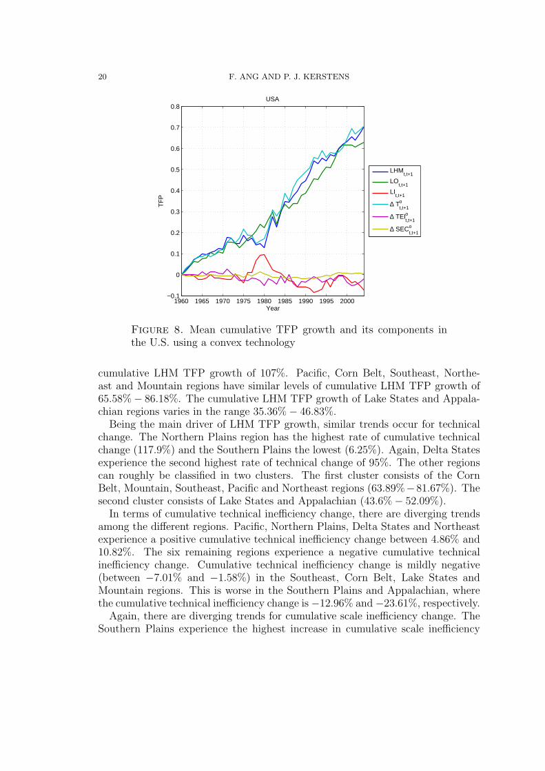
Our main finding for the U.S. as a whole is that LHM TFP clearly increases overtime. The LHM TFP indicator increases by 70.46% between 1960 and 2004. Thisboils down to an average LHM TFP growth of 1.60% per year. LHM TFP growthis driven by output growth (+62.98%) rather than input decline (−7.47%). In theperiod 1977 − 1982, LIt,t+1 contributes to a temporary slowdown in LHM TFPgrowth. LIt,t+1 only plays a minor role in the remaining periods.We now turn to our LHM decomposition. Our decomposition shows that techni-

cal change (+70.55%) is the main driver, while technical inefficiency change (−1.99%)and scale inefficiency change (+0.42%) only play a minor role. Table 4 summarizes

14Infeasibilities may arise for the components where the year of the observation differs fromthe year of the reference technology. As there is no easy solution to solve this problem,Briec and Kerstens (2009) recommend to report the infeasibilities. There were only infeasibi-lities for Rhode Island.


1960 1965 1970 1975 1980 1985 1990 1995 2000−0.06

−0.04

−0.02

0

0.02

0.04

0.06

0.08

Year

TF

P

USA

LHMt,t+1

Figure 7. Mean TFP change in the U.S. using a convex technology

these results and lists the minimal and maximal values of the LHM TFP indica-tor and its components per subperiod of 11 years. It also lists the correspondingstates.

LHMt,t+1 LOt,t+1 LIt,t+1 ∆T ot,t+1

∆TEIot,t+1∆SECo

t,t+1∑2004t=1960

mean(states) 70.46 62.98 -7.47 70.55 -1.99 0.42

Avg growth rate 1.60 1.43 -0.17 1.60 -0.05 9.50 ×10−3

min

1960/71 -4.37 (OK) -3.84 (NJ) -6.61 (RI) -3.83 (OK) -1.60 (OK) -3.32 (NV)

1971/82 -1.28 (WV) -1.55 (MO) -1.84 (RI) -0.67 (FL) -2.92 (WY) -1.65 (DE)

1982/93 -0.36 (TN) -1.53 (NH) -3.52 (KS) 0.64 (FL) -2.64 (MO) -1.63 (SD)1993/04 -2.41 (WY) -2.34 (WY) -2.70 (RI) -1.34 (KY) -3.65 (WY) -0.93 (LA)

max

1960/71 7.16 (ND) 7.21 (AR) 3.18 (AR) 5.42 (NV) 3.72 (ND) 1.76 (LA)1971/82 3.77 (IL) 3.51 (WA) 2.63 (DE) 4.05 (ND) 1.59 (OK) 1.33 (OR)

1982/93 5.64 (DE) 4.83 (WV) 1.99 (OK) 5.67 (DE) 3.62 (MT) 2.03 (IA)

1993/04 4.24 (AL) 4.11 (SD) 2.53 (KY) 4.38 (MS) 2.89 (MO) 2.54 (TN)

Table 4. TFP growth and its components in the U.S. covering theyears 1960− 2004 (in %) using a convex technology

4.3.2. Main findings per region. Figure 9 depicts the mean cumulative LHM TFPand its components for every region over time. The mean is computed with re-spect to all states in that particular agricultural production region. The NorthernPlains experienced the highest cumulative LHM TFP growth (119.3%) while theSouthern Plains experienced the lowest cumulative LHM TFP growth (8.96%)over the entire period. Between them, Delta States experience the second highest


1960 1965 1970 1975 1980 1985 1990 1995 2000−0.1

0

0.1

0.2

0.3

0.4

0.5

0.6

0.7

0.8

Year

TF

P

USA

LHMt,t+1

LOt,t+1

LIt,t+1

∆ Tt,t+1o

∆ TEIt,t+1o

∆ SECt,t+1o

Figure 8. Mean cumulative TFP growth and its components inthe U.S. using a convex technology

cumulative LHM TFP growth of 107%. Pacific, Corn Belt, Southeast, Northe-ast and Mountain regions have similar levels of cumulative LHM TFP growth of65.58%− 86.18%. The cumulative LHM TFP growth of Lake States and Appala-chian regions varies in the range 35.36%− 46.83%.Being the main driver of LHM TFP growth, similar trends occur for technical

change. The Northern Plains region has the highest rate of cumulative technicalchange (117.9%) and the Southern Plains the lowest (6.25%). Again, Delta Statesexperience the second highest rate of technical change of 95%. The other regionscan roughly be classified in two clusters. The first cluster consists of the CornBelt, Mountain, Southeast, Pacific and Northeast regions (63.89%−81.67%). Thesecond cluster consists of Lake States and Appalachian (43.6%− 52.09%).In terms of cumulative technical inefficiency change, there are diverging trends

among the different regions. Pacific, Northern Plains, Delta States and Northeastexperience a positive cumulative technical inefficiency change between 4.86% and10.82%. The six remaining regions experience a negative cumulative technicalinefficiency change. Cumulative technical inefficiency change is mildly negative(between −7.01% and −1.58%) in the Southeast, Corn Belt, Lake States andMountain regions. This is worse in the Southern Plains and Appalachian, wherethe cumulative technical inefficiency change is−12.96% and−23.61%, respectively.Again, there are diverging trends for cumulative scale inefficiency change. The

Southern Plains experience the highest increase in cumulative scale inefficiency


change (15.67%) followed closely by the Appalachian region (15.38%). The Nort-hern Plains experience a negative cumulative scale inefficiency change (−9.5%).Between these extremes, the Pacific, Corn Belt, Delta States, Southeast andLake States have a positive cumulative scale inefficiency change in the range of1.29%− 7.56%. In contrast, the cumulative scale inefficiency change of the Nort-heast and Mountain regions is negative (−6.64% and −7.88%, respectively).

1960 1970 1980 1990 2000−0.4

−0.2

0

0.2

0.4

0.6

0.8

1

1.2

Year

TF

P

TFP growth in the USA


(a) Average cumulative TFP growthper region

1960 1970 1980 1990 2000−0.4

−0.2

0

0.2

0.4

0.6

0.8

1

1.2

Year

TF

P

Technical change in the USA


(b) Average cumulative technicalchange per region

1960 1970 1980 1990 2000−0.4

−0.3

−0.2

−0.1

0

0.1

0.2

0.3

Year

TF

P

Technical inefficiency change in the USA


(c) Average cumulative technical inef-ficiency change per region

1960 1970 1980 1990 2000−0.15

−0.1

−0.05

0

0.05

0.1

0.15

0.2

Year

TF

P

Scale inefficiency change in the USA


(d) Average cumulative scale ineffi-ciency change per region

Figure 9. Cumulative TFP growth and its decomposition per U.S.region using a convex technology

Although all U.S. regions experienced LHM TFP growth in the period 1960 −2004, this analysis shows that the contribution of the underlying factors variesconsiderably per region. Technical change is the main driver of LHM TFP growthfor all U.S. regions. In addition, several U.S. regions partly increased TFP by


becoming more efficient over time and/or operating at a more optimal scale. Otherregions mainly relied on technical change to increase LHM TFP.

4.4. Discussion. The results depend on the convexity assumption of the techno-logy. We test the hypothesis whether the distributions of the LHM TFP indica-tor and its components for FDH and DEA are not significantly different using aKolmogorov-Smirnov test. This nonparametrically tests the hypothesis H0 whet-her two samples are drawn from the same underlying distribution. We conduct thetest for every year separately, resulting in 44 different test hypotheses for everycomponent. The results at the 10% significance level are presented in Table 5.For the majority of years, the distributions of the LHMt,t+1 and its componentsLOt,t+1 and LIt,t+1 are not statistically different using FDH and DEA. In contrast,the distributions of ∆T o

t,t+1 are statistically significant for a majority of years andthe distributions of ∆TEIot,t+1 and ∆SECo

t,t+1 under both technologies are signifi-cantly different for all years. These results in conjunction with Table 3 and Table 4lead us to the following qualitative conclusions.

LHMt,t+1 LOt,t+1 LIt,t+1 ∆T ot,t+1 ∆TEIot,t+1 ∆SECo

t,t+1

Reject H0 per year at 10% 9/44 12/44 8/44 25/44 44/44 44/44Reject H0 at 10% No Yes Yes Yes Yes Yes

Table 5. Results of Kolmogorov-Smirnov test testing equality ofdistributions under non-convex and convex technologies

Both results suggest there is substantial LHM TFP growth over the entire periodwhich is mainly driven by technical progress. Both the DEA and FDH resultsindicate that output growth dominates input decline, although this finding is muchmore pronounced for the DEA results. A possible explanation for the smallercontribution of input decline is that some quasi-fixed inputs (e.g. land) are notconstantly adjusted over time or that input reduction is not an objective for someinputs such as land and labor.We analyze LHM TFP growth and technical change across time, farm types and

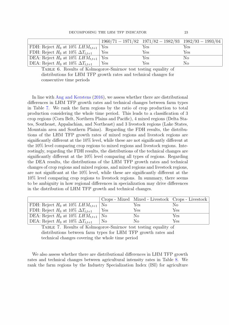
agricultural intensity rates. Table 6 shows the results of the Kolmogorov-Smirnovtest testing equality of distributions for LHM TFP growth rates and technicalchanges for consecutive subperiods of eleven years in line with Table 3. RegardingFDH, all distributions of consecutive LHM TFP growth rates and technical changesare significantly different at the 10% level. Regarding DEA, the distributions ofthe LHM TFP growth rates and technical changes between 1982/93 and 1993/04are not significantly different at the 10% level, while these are significantly differentcomparing the preceding time periods. This suggests that distributional differencesin productivity growth driven by shifts in technology may decrease in importancethroughout time.


1960/71− 1971/82 1971/82− 1982/93 1982/93− 1993/04FDH: Reject H0 at 10% LHMt,t+1 Yes Yes YesFDH: Reject H0 at 10% ∆Tt,t+1 Yes Yes YesDEA: Reject H0 at 10% LHMt,t+1 Yes Yes NoDEA: Reject H0 at 10% ∆Tt,t+1 Yes Yes No

Table 6. Results of Kolmogorov-Smirnov test testing equality ofdistributions for LHM TFP growth rates and technical changes forconsecutive time periods

In line with Ang and Kerstens (2016), we assess whether there are distributionaldifferences in LHM TFP growth rates and technical changes between farm typesin Table 7. We rank the farm regions by the ratio of crop production to totalproduction considering the whole time period. This leads to a classification of 3crop regions (Corn Belt, Northern Plains and Pacific), 4 mixed regions (Delta Sta-tes, Southeast, Appalachian, and Northeast) and 3 livestock regions (Lake States,Mountain area and Southern Plains). Regarding the FDH results, the distribu-tions of the LHM TFP growth rates of mixed regions and livestock regions aresignificantly different at the 10% level, while these are not significantly different atthe 10% level comparing crop regions to mixed regions and livestock regions. Inte-restingly, regarding the FDH results, the distributions of the technical changes aresignificantly different at the 10% level comparing all types of regions. Regardingthe DEA results, the distributions of the LHM TFP growth rates and technicalchanges of crop regions and mixed regions, and mixed regions and livestock regions,are not significant at the 10% level, while these are significantly different at the10% level comparing crop regions to livestock regions. In summary, there seemsto be ambiguity in how regional differences in specialization may drive differencesin the distribution of LHM TFP growth and technical changes.

Crops - Mixed Mixed - Livestock Crops - LivestockFDH: Reject H0 at 10% LHMt,t+1 No Yes NoFDH: Reject H0 at 10% ∆Tt,t+1 Yes Yes YesDEA: Reject H0 at 10% LHMt,t+1 No No YesDEA: Reject H0 at 10% ∆Tt,t+1 No No Yes

Table 7. Results of Kolmogorov-Smirnov test testing equality ofdistributions between farm types for LHM TFP growth rates andtechnical changes covering the whole time period

We also assess whether there are distributional differences in LHM TFP growthrates and technical changes between agricultural intensity rates in Table 8. Werank the farm regions by the Industry Specialization Index (ISI) for agriculture


considering 1963− 200415. The U.S. Bureau of Economic Analysis (BEA) compu-tes the ISI as the agricultural industry’s share of the state-level Gross DomesticProduct divided by the agricultural industry’s share of the U.S. total for the samestatistic. The complete dataset can be found in BEA (2016). We rank the regionsby ISI, which leads to a classification of 3 low ISI regions (Northeast, Lake Statesand Southeast), 4 medium ISI regions (Appalachian, Southern Plains, Pacific andCorn Belt) and 3 high ISI regions (Mountain area, Delta States and NorthernPlains). With respect to the FDH results, comparing distributions of the LHMTFP growth rates for all groups do not yield any significant difference at the 10%level. The distributions of the technical changes are significantly different at the10% level comparing low ISI regions to medium and high ISI regions. Regardingthe DEA results, the distributions of the LHM TFP growth rates and technicalchanges are significantly different at the 10% level comparing medium ISI regionsto high ISI regions. Similar to the preceding section, there thus seems to be am-biguity in how regional differences in agricultural intensity may drive differencesin the distribution of LHM TFP growth and technical changes.

Low - Medium Medium - High Low - HighFDH: Reject H0 at 10% LHMt,t+1 No No NoFDH: Reject H0 at 10% ∆Tt,t+1 Yes No YesDEA: Reject H0 at 10% LHMt,t+1 No Yes NoDEA: Reject H0 at 10% ∆Tt,t+1 No Yes No

Table 8. Results of Kolmogorov-Smirnov test testing equality ofdistributions between agricultural intensity rates for LHM TFP gro-wth rates and technical changes covering the whole time period

The contribution of technical inefficiency change to LHM TFP growth is lessclear-cut. Using FDH, technical inefficiency change is virtually nonexistent. Furt-her inspection reveals that most (contemporaneous) technical inefficiency scoresare zero using FDH. This drives the extremely low technical inefficiency change.Therefore, these remarkable results may be due to lower discriminatory power ofFDH in this case since there are relatively few observations per year comparedto the number of inputs and outputs. Using DEA, there is a small cumulativeincrease in technical inefficiency change.The results differ more for the scale inefficiency change component. There is

a substantial increase in cumulative scale inefficiency change using FDH, whereasthere is almost no cumulative scale inefficiency change using DEA. Again, thismay be due to the higher discriminatory power of DEA.Our DEA results are in line with other empirical studies that analyze the TFP

growth in the U.S. agricultural sector using the same data source. Zofıo and Lovell

15Data for 1960− 1962 are unavailable.


(2001), Ball et al. (2010), O’Donnell (2012b) and Ball et al. (2016) also find sub-stantial TFP growth16. It is driven by technical progress rather than efficiencychange in line with Zofıo and Lovell (2001) and Ball et al. (2016). FollowingBall et al. (2016), TFP growth is also due to output growth rather than chan-ges in the input level.

5. Conclusions

This paper decomposes the additively complete LHM TFP indicator into com-ponents of technical change, technical inefficiency change and scale inefficiencychange. Our approach is general in that it does not require differentiability orconvexity of the production technology. Using a nonparametric framework, theempirical application focuses on state-level data of the U.S. agricultural sectorover the period 1960−2004. We compute the scores using FDH and DEA to showthe flexibility of our decomposition and to investigate the potential issue of non-convexities in the agricultural sector. Furthermore, we analyze LHM TFP growthand technical change across time, farm types and agricultural intensity rates.The FDH results show that LHM TFP has increased by 78.61% in the consi-

dered period. This is due to output growth (+44.10%) as well as input decline(−34.51%). Technical change (+130.57%) and scale inefficiency change (−60.63%)are the main drivers, while technical inefficiency change (−0.32%) only plays a mi-nor role.Following the DEA results, LHM TFP has increased by 70.46% for the conside-

red period. This productivity growth is due to output growth (+62.98%) ratherthan changes in the input level (−7.47%). Technical change is the main dri-ver (+70.55%), while technical inefficiency change (−1.99%) and scale inefficiencychange (+0.42%) only play a minor role.The results thus depend on whether we use FDH or DEA. Although this may

partly be driven by the underlying true production technology, we note that FDHmay result in too low discriminatory power to compute the distance functionsgiven the relatively low number of observations for the number of variables in thisapplication.Following the Kolmogorov-Smirnov tests, there seem to be differences in the dis-

tributions of LHM TFP growth and technical change across time, farm types andagricultural intensity rates. We suspect that policy instruments and factor endo-wments (e.g. soil and weather conditions) may drive differences across time, farmtypes and agricultural intensity rates, potentially resulting in differing distributi-ons in LHM TFP growth and technical change. For instance, agricultural supportpayments with restrictions on land use (Just and Kropp, 2013) and ethanol subsi-dies (Motamed et al., 2016) likely have an impact on geographical specialization.

16Zofıo and Lovell (2001) only analyze TFP growth over the period 1960− 1990.


This information would be relevant for policy makers. Such an empirical investi-gation is left for future research.


References

Ang, F. and P. J. Kerstens (2016): “To Mix or Specialise? A CoordinationProductivity Indicator for English and Welsh farms,” Journal of Agricultural

Economics, 67, 779–798.Aragon, Y., A. Daouia, and C. Thomas-Agnan (2005): “NonparametricFrontier Estimation: A Conditional Quantile-Based Approach,” Econometric

Theory, 21, 358–389.Balk, B. M., R. Fare, and S. Grosskopf (2003): “The theory of economicprice and quantity indicators,” Economic Theory, 23, 149–164.

Ball, E., S. L. Wang, and R. Nehring (2016): “USDA ERS - AgriculturalProductivity in the U.S.” (Accessed on 2016-05-02).

Ball, V. E., R. Fare, S. Grosskopf, and D. Margaritis (2010): The

Economic Impact of Public Support to Agriculture, New York, NY: SpringerNew York, chap. Productivity and Profitability of US Agriculture: Evidencefrom a Panel of States, 125–139.

Barros, C. P., A. Ibiwoye, and S. Managi (2008): “Productivity changeof Nigerian insurance companies: 1994–2005,” African Development Review, 20,505–528.

BEA (2016): “BEA,” http://http://www.bea.gov/iTable/index_regional.

cfm, (Accessed on 2016-12-01).Bjurek, H. (1996): “The Malmquist total factor productivity index,” Scandina-

vian Journal of Economics, 303–313.Bogetoft, P. (1996): “DEA on relaxed convexity assumptions,” Management

Science, 42, 457–465.Bogetoft, P. and L. Otto (2015): Benchmarking with DEA and SFA, rpackage version 0.26.

Briec, W. and K. Kerstens (2004): “A Luenberger-Hicks-Moorsteen producti-vity indicator: its relation to the Hicks-Moorsteen productivity index and theLuenberger productivity indicator,” Economic Theory, 23, 925–939.

——— (2009): “Infeasibility and directional distance functions with applicationto the determinateness of the Luenberger productivity indicator,” Journal of

Optimization Theory and Applications, 141, 55–73.Briec, W., K. Kerstens, and N. Peypoch (2012): “Exact relations betweenfour definitions of productivity indices and indicators,” Bulletin of Economic

Research, 64, 265–274.Briec, W. and Q. B. Liang (2011): “On some semilattice structures for pro-duction technologies,” European Journal of Operational Research, 215, 740–749.

Briec, W. and N. Peypoch (2007): “Biased technical change and parallelneutrality,” Journal of Economics, 92, 281–292.

Caves, D. W., L. R. Christensen, and W. E. Diewert (1982): “The eco-nomic theory of index numbers and the measurement of input, output, andproductivity,” Econometrica, 1393–1414.

http://http://www.bea.gov/iTable/index_regional.cfm

http://http://www.bea.gov/iTable/index_regional.cfm


Cazals, C., J.-P. Florens, and L. Simar (2002): “Nonparametric frontierestimation: a robust approach,” Journal of Econometrics, 106, 1 – 25.

Chambers, R. G. (2002): “Exact nonradial input, output, and productivitymeasurement,” Economic Theory, 20, 751–765.

Chambers, R. G., R. Fare, and S. Grosskopf (1996): “Productivity growthin APEC countries,” Pacific Economic Review, 1, 181–190.

Cherchye, L., T. Kuosmanen, and T. Post (2001): “FDH directional dis-tance functions with an application to European commercial banks,” Journal of

Productivity Analysis, 15, 201–215.Daraio, C. and L. Simar (2016): “Efficiency and benchmarking with directi-onal distances: a data-driven approach,” Journal of the Operational Research

Society, 67, 928–944.Diewert, W. E. (1976): “Exact and superlative index numbers,” Journal of

Econometrics, 4, 115–145.Diewert, W. E. and K. J. Fox (2014): “Reference technology sets, Free Dis-posal Hulls and productivity decompositions,” Economics Letters, 122, 238–242.

——— (2017): “Decomposing productivity indexes into explanatory factors,” Eu-

ropean Journal of Operational Research, 256, 275 – 291.Epure, M. (2016): “Benchmarking for routines and organizational knowledge: amanagerial accounting approach with performance feedback,” Journal of Pro-

ductivity Analysis, 46, 87–107.Epure, M., K. Kerstens, and D. Prior (2011): “Bank productivity andperformance groups: A decomposition approach based upon the Luenbergerproductivity indicator,” European Journal of Operational Research, 211, 630–641.

Fare, R., S. Grosskopf, and D. Njinkeu (1988): “Note—On Piecewise Re-ference Technologies,” Management Science, 34, 1507–1511.

Fare, R., S. Grosskopf, M. Norris, and Z. Zhang (1994): “Productivitygrowth, technical progress, and efficiency change in industrialized countries,”American Economic Review, 66–83.

Fare, R., S. Grosskopf, and P. Roos (1998): “Malmquist productivity in-dexes: a survey of theory and practice,” in Index numbers: Essays in honour of

Sten Malmquist, Springer, 127–190.Grosskopf, S. (2003): “Some remarks on productivity and its decompositions,”Journal of Productivity Analysis, 20, 459–474.

Just, D. R. and J. D. Kropp (2013): “Production Incentives from Static De-coupling: Land Use Exclusion Restrictions,” American Journal of Agricultural

Economics, 95, 1049–1067.Luenberger, D. G. (1992): “New optimality principles for economic efficiencyand equilibrium,” Journal of optimization theory and applications, 75, 221–264.

Managi, S. (2010): “Productivity measures and effects from subsidies and trade:an empirical analysis for Japan’s forestry,” Applied Economics, 42, 3871–3883.


Motamed, M., L. McPhail, and R. Williams (2016): “Corn Area Responseto Local Ethanol Markets in the United States: A Grid Cell Level Analysis,”American Journal of Agricultural Economics, 98, 726–743.

Nakano, M. and S. Managi (2008): “Regulatory reforms and productivity:an empirical analysis of the Japanese electricity industry,” Energy Policy, 36,201–209.

O’Donnell, C. J. (2012a): “An aggregate quantity framework for measuringand decomposing productivity change,” Journal of Productivity Analysis, 38,255–272.

——— (2012b): “Nonparametric estimates of the components of productivity andprofitability change in US agriculture,” American Journal of Agricultural Eco-

nomics, 873–890.Petersen, N. C. (1990): “Data envelopment analysis on a relaxed set of as-sumptions,” Management Science, 36, 305–314.

Podinovski, V. (2005): “Selective convexity in DEA models,” European Journal

of Operational Research, 161, 552–563.Tulkens, H. (1993): “On FDH Efficiency Analysis: Some Methodological Issuesand Applications to Retail Banking, Courts, and Urban Transit,” Journal of

Productivity Analysis, 183–210.USDA (2016): “USDA,” http://www.ers.usda.gov/data-products/

agricultural-productivity-in-the-us.aspx, (Accessed on 2016-11-24).Zofıo, J. L. and C. A. K. Lovell (2001): “Graph efficiency and productivitymeasures: an application to US agriculture,” Applied Economics, 33, 1433–1442.

http://www.ers.usda.gov/data-products/agricultural-productivity-in-the-us.aspx

http://www.ers.usda.gov/data-products/agricultural-productivity-in-the-us.aspx


Appendix A. Managi (2010)’s decomposition

Managi (2010) decomposes the Luenberger-Hicks-Moorsteen indicator into techni-cal change (TC):

TC =[

Dt+1(xt+1,yt+1; (git+1, 0))−Dt(xt+1,yt+1; (g

it+1, 0))

]

−[

Dt+1(xt+1,yt+1; (0,got+1))−Dt(xt+1,yt+1; (0,g

ot+1))

]

,

and the residual being efficiency change (EC):

EC =1

2

{


ot+1))

− Dt(xt+1,yt; (git+1, 0)) +Dt(xt,yt; (g

it, 0))

+ Dt+1(xt+1,yt; (0,got )) +Dt+1(xt+1,yt+1; (0,g

ot+1))

− Dt+1(xt+1,yt+1; (git+1, 0)) +Dt+1(xt,yt+1; (g

it, 0))

}

−Dt(xt+1,yt+1; (0,got+1))−Dt+1(xt+1,yt+1; (g

it+1, 0)) +Dt(xt+1,yt+1; (g

it+1, 0))

However, this decomposition is incomplete. First, it lacks a scale (in)efficiencychange component. Second, there is no reason for TC to be defined as a differencebetween an output-oriented technical change component and an input-orientedtechnical change component. Furthermore, TC is only defined with respect toobservations in period t + 1, although there is no clear reason to favor those toobservations in period t. Finally, the EC component does not capture technical(in)efficiency change.

Appendix B. Decomposition using the input direction

The decomposition using the input direction is:

(B.1) LHMt,t+1 = ∆T i +∆TEI i +∆SEC i,

representing technical change, technical inefficiency change and scale inefficiencychange, respectively.The technical change component is defined as:

∆T i =1

2

{[

Dt+1(xt,yt; (git, 0))−Dt(xt,yt; (g

it, 0))

]

+[

Dt+1(xt+1,yt+1; (git+1, 0))−Dt(xt+1,yt+1; (g

it+1, 0))

]}

,(B.2)

and the same interpretation as before. Technical inefficiency change is:

∆TEI i = Dt(xt,yt; (git, 0))−Dt+1(xt+1,yt+1; (g

it+1, 0)).(B.3)


From the residual

LHMt,t+1−∆T i −∆TEI i =(B.4)

1

2

{[


ot+1))

]

+[


ot+1))

]}

−1

2

{[

Dt(xt+1,yt; (git+1, 0))−Dt(xt+1,yt+1; (g

it+1, 0))

]

+[

Dt+1(xt,yt; (git, 0))−Dt+1(xt,yt+1; (g

it, 0))

]}

,

we recover the scale inefficiency change component in a similar way as before.Define the projections of xt and xt+1 on the production frontier at time t:

x∗t = xt −Dt(xt,yt; (g

it, 0))g

it(B.5a)

x∗∗t+1 = xt+1 −Dt(xt+1,yt+1; (g

it+1, 0))g

it+1,(B.5b)

and the projections of xt and xt+1 on the production frontier at time t+ 1:

x∗∗t = xt −Dt+1(xt,yt; (g

it, 0))g

it(B.6a)

x∗t+1 = xt+1 −Dt+1(xt+1,yt+1; (g

it+1, 0))g

it+1.(B.6b)

Respectively adding and subtractingDt(xt,yt; (git, 0)) andDt+1(xt+1,yt+1; (g

it+1, 0))

to and from (B.4), and using the translation property of the directional distancefunction and the definitions of the projections above, we find the scale inefficiencychange component:

∆SEC i =1

2

{[


ot+1))

]

(B.7)

−[

Dt(x∗∗t+1,yt; (g

it+1, 0))−Dt(x

∗t ,yt; (g

it, 0))

]

+[


ot+1))

]

−[

Dt+1(x∗t+1,yt+1; (g

it+1, 0))−Dt+1(x

∗∗t ,yt+1; (g

it, 0))

]}

≡1

2

{

∆SEC it +∆SEC i

t+1

}

.

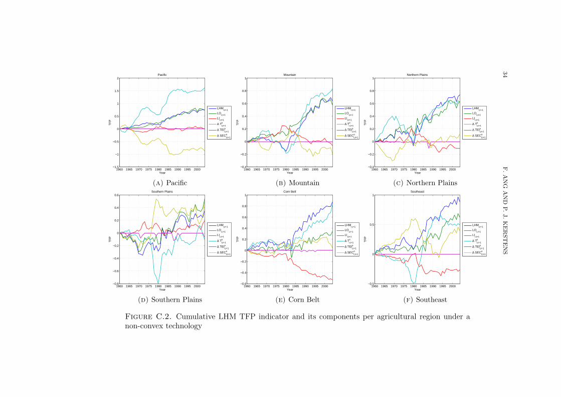
Appendix C. State-level TFP figures

This appendix includes the LHM TFP indicator and its components per agri-cultural region. Each figure is constructed by averaging over all states in thatparticular agricultural region in every year.

C.1. Convex technology.

32

F.ANG

AND

P.J.KERSTENS

1960 1965 1970 1975 1980 1985 1990 1995 2000−0.2

0

0.2

0.4

0.6

0.8

1

1.2

Year

TF

P

Pacific

LHMt,t+1

LOt,t+1

LIt,t+1

∆ Tt,t+1o

∆ TEIt,t+1o

∆ SECt,t+1o

(a) Pacific

1960 1965 1970 1975 1980 1985 1990 1995 2000−0.2

0

0.2

0.4

0.6

0.8

1

1.2

Year

TF

P

Mountain

LHMt,t+1

LOt,t+1

LIt,t+1

∆ Tt,t+1o

∆ TEIt,t+1o

∆ SECt,t+1o

(b) Mountain

1960 1965 1970 1975 1980 1985 1990 1995 2000−0.4

−0.2

0

0.2

0.4

0.6

0.8

1

1.2

Year

TF

P

Northern Plains

LHMt,t+1

LOt,t+1

LIt,t+1

∆ Tt,t+1o

∆ TEIt,t+1o

∆ SECt,t+1o

(c) Northern Plains

1960 1965 1970 1975 1980 1985 1990 1995 2000−0.4

−0.3

−0.2

−0.1

0

0.1

0.2

0.3

0.4

0.5

0.6

Year

TF

P

Southern Plains

LHMt,t+1

LOt,t+1

LIt,t+1

∆ Tt,t+1o

∆ TEIt,t+1o

∆ SECt,t+1o

(d) Southern Plains

1960 1965 1970 1975 1980 1985 1990 1995 2000−0.4

−0.2

0

0.2

0.4

0.6

0.8

1

Year

TF

P

Corn Belt

LHMt,t+1

LOt,t+1

LIt,t+1

∆ Tt,t+1o

∆ TEIt,t+1o

∆ SECt,t+1o

(e) Corn Belt

1960 1965 1970 1975 1980 1985 1990 1995 2000−0.1

0

0.1

0.2

0.3

0.4

0.5

0.6

0.7

0.8

0.9

Year

TF

P

Southeast

LHMt,t+1

LOt,t+1

LIt,t+1

∆ Tt,t+1o

∆ TEIt,t+1o

∆ SECt,t+1o

(f) Southeast

Figure C.1. Cumulative LHM TFP indicator and its components per agricultural region under aconvex technology


1960 1965 1970 1975 1980 1985 1990 1995 2000−0.6

−0.4

−0.2

0

0.2

0.4

0.6

0.8

Year

TF

P

Northeast

LHMt,t+1

LOt,t+1

LIt,t+1

∆ Tt,t+1o

∆ TEIt,t+1o

∆ SECt,t+1o

(g) Northeast

1960 1965 1970 1975 1980 1985 1990 1995 2000−0.2

−0.1

0

0.1

0.2

0.3

0.4

0.5

0.6

Year

TF

P

Lake States

LHMt,t+1

LOt,t+1

LIt,t+1

∆ Tt,t+1o

∆ TEIt,t+1o

∆ SECt,t+1o

(h) Lake States

1960 1965 1970 1975 1980 1985 1990 1995 2000−0.3

−0.2

−0.1

0

0.1

0.2

0.3

0.4

0.5

0.6

0.7

Year

TF

P

Appalachian

LHMt,t+1

LOt,t+1

LIt,t+1

∆ Tt,t+1o

∆ TEIt,t+1o

∆ SECt,t+1o

(i) Appalachian

1960 1965 1970 1975 1980 1985 1990 1995 2000−0.2

0

0.2

0.4

0.6

0.8

1

1.2

1.4

Year

TF

PDelta States

LHMt,t+1

LOt,t+1

LIt,t+1

∆ Tt,t+1o

∆ TEIt,t+1o

∆ SECt,t+1o

(j) Delta States

Figure C.1. Cumulative LHM TFP indicator and its componentsper agricultural region under a convex technology

C.2. Non-convex technology.

34

F.ANG

AND

P.J.KERSTENS

1960 1965 1970 1975 1980 1985 1990 1995 2000−1.5

−1

−0.5

0

0.5

1

1.5

2

Year

TF

P

Pacific

LHMt,t+1

LOt,t+1

LIt,t+1

∆ Tt,t+1o

∆ TEIt,t+1o

∆ SECt,t+1o

(a) Pacific

1960 1965 1970 1975 1980 1985 1990 1995 2000−0.4

−0.2

0

0.2

0.4

0.6

0.8

1

Year

TF

P

Mountain

LHMt,t+1

LOt,t+1

LIt,t+1

∆ Tt,t+1o

∆ TEIt,t+1o

∆ SECt,t+1o

(b) Mountain

1960 1965 1970 1975 1980 1985 1990 1995 2000−0.4

−0.2

0

0.2

0.4

0.6

0.8

1

Year

TF

P

Northern Plains

LHMt,t+1

LOt,t+1

LIt,t+1

∆ Tt,t+1o

∆ TEIt,t+1o

∆ SECt,t+1o

(c) Northern Plains

1960 1965 1970 1975 1980 1985 1990 1995 2000−0.8

−0.6

−0.4

−0.2

0

0.2

0.4

0.6

Year

TF

P

Southern Plains

LHMt,t+1

LOt,t+1

LIt,t+1

∆ Tt,t+1o

∆ TEIt,t+1o

∆ SECt,t+1o

(d) Southern Plains

1960 1965 1970 1975 1980 1985 1990 1995 2000−0.6

−0.4

−0.2

0

0.2

0.4

0.6

0.8

1

Year

TF

P

Corn Belt

LHMt,t+1

LOt,t+1

LIt,t+1

∆ Tt,t+1o

∆ TEIt,t+1o

∆ SECt,t+1o

(e) Corn Belt

1960 1965 1970 1975 1980 1985 1990 1995 2000−0.5

0

0.5

1

Year

TF

P

Southeast

LHMt,t+1

LOt,t+1

LIt,t+1

∆ Tt,t+1o

∆ TEIt,t+1o

∆ SECt,t+1o

(f) Southeast

Figure C.2. Cumulative LHM TFP indicator and its components per agricultural region under anon-convex technology


1960 1965 1970 1975 1980 1985 1990 1995 2000−3

−2

−1

0

1

2

3

4

Year

TF

P

Northeast

LHMt,t+1

LOt,t+1

LIt,t+1

∆ Tt,t+1o

∆ TEIt,t+1o

∆ SECt,t+1o

(g) Northeast

1960 1965 1970 1975 1980 1985 1990 1995 2000−0.6

−0.4

−0.2

0

0.2

0.4

0.6

0.8

1

1.2

Year

TF

P

Lake States

LHMt,t+1

LOt,t+1

LIt,t+1

∆ Tt,t+1o

∆ TEIt,t+1o

∆ SECt,t+1o

(h) Lake States

1960 1965 1970 1975 1980 1985 1990 1995 2000−0.6

−0.4

−0.2

0

0.2

0.4

0.6

0.8

Year

TF

P

Appalachian

LHMt,t+1

LOt,t+1

LIt,t+1

∆ Tt,t+1o

∆ TEIt,t+1o

∆ SECt,t+1o

(i) Appalachian

1960 1965 1970 1975 1980 1985 1990 1995 2000−0.4

−0.2

0

0.2

0.4

0.6

0.8

1

Year

TF

PDelta States

LHMt,t+1

LOt,t+1

LIt,t+1

∆ Tt,t+1o

∆ TEIt,t+1o

∆ SECt,t+1o

(j) Delta States

Figure C.2. Cumulative LHM TFP indicator and its componentsper agricultural region under a non-convex technology

decomposing the luenberger-hicks-moorsteen total …

Documents