Indian Journal or Pure & A ppli ed Phys ics Vol. 37. September 1999. pp. 667-675

Decomposition of dielectric dispersion into debye domains

B Hemalatha * . V G R aul & Y P Singh2

Department of Electrical Engineer ing. Indian Institute or Technology. Kharagpur 721 302

Received 23 October I 99l:i: rev ised 29 December 1998: accepted 26 July 199LJ

Th is paper presents a Genera l M ode l. based on a systems approach for representing the dielectric response or a system

possessi ng two or more distinct absorpti on regions. A novel method for determining the minimum number of secti ons in the

model and the estimati on of the model parameters bas been proposed. First the minimum number of model secti ons which can

best descr ibe the response data is round either by using Levy ' s complex curve fitting technique or a M onte Carlo search procedure.

With thi s information, the model parameters are accurately es timated by the minimization of an error function. using the Neider

- M ead Simplex algorithm. The proposed methodology includes two important cases. namely. when both the real and imaginary

part or the response is kn own and whcn onl y the imaginnry part of thc response is known. Several illustra ti ve ex amples arc

presented.

1 Introduction The di e lectri c re laxati on spectrum of seve ral linear

d ie lectri cs , parti cul arl y the die lectri c liquids and liquid

mi xtures in the mi c rowave range are known to possess

di stinct absorpti on regions I . In such cases, the re laxati on

spectrum is decomposed into di stinct number of Debye

domains. When two absorption regio ns are known to

ex ist, g raphical me th ods like that due to Davidson and

Co le2.:l ha ve been used fo r separation of the loss peaks.

For three di spe rs ion regions. the use of Fl etcher-Powell

al go rithm for separatio n of the loss peaks was described

by Salefran4 The di sad vantage of thi s method is that it

requires both £, and £= to be kn own apri o ri . In additi on,

the nume rical methods';'(' proposed so far for deco mpo­

siti on are hi ghl y sensiti ve to the initi a l values used . Based on a systems approach, thi s pape r proposes a

gene ral mode l fo r describin g the die lectric respon se of

a syste m hav ing 11 d isti nct absorpti on regions 7 Thi s

pape r desc ribes a syste matic procedure for decompos in g

the response data into appropriate number of Debye

do main s . The f irst step decides the numbe r of Debye

sections and the approx imate magnitudes of the parame­

te r values. The second step performs the minimi zati on

whi ch es timates the magnitudes of the re fined di spe r­

sion paramete rs. T wo impo rt ant cases have been cons id­

e reel , th at is, when both £' ( real part of pe rmitti v ity) and

£" (i mag i nary pa rt of pe rmitti v ity) a re ava i lable and that

whe n onl y £" is a vailable.

2 Model for a Dielectric Possessing Multiple

Absorptions

For a linear die lectri c system in gene ra l, £*(s) can be

re presented in the Laplace domain as :

P ( S) £* ( 5) =--

Q (.I' ) ... ( I )

where pes) and Q (s ) are polynomial s of the complex

ope rator 5: 2 z· 1 z pes) = ao + al s + a 2S + ... . +az. ls + azs .

Q( .) - I l b .2 b jI·1 I JI .\ - + 'h~ + 2·\ + .. .. . + /1. 1.1 + )//.1

.. (2) .. .(3)

The roots of the denominator po lyno mi a l g i ve the

trans iti on frequenc ies and hence the re laxati on times.

For phys ical syste m p 2:::.. Since di e lec tri c systems have

finite £, and ~, the numerato r and denominator polyno­

mia l have the same order. Thus, p = z = n and the

permitti vity functi on of the die lectri c is of the fo rm :

2 1/ - I /I

( ao + al s + a2S + ... + all- IS + (I"S

£ * s) = -------------- ... (4) 2 /1 - I /I

I+bls + b2s + .. .+ b,,_IS + b"s

Therefore, the paramete rs £, and £N. are writren as:

E, = lim £ * ( s ) = on ... (5) .1-->0

. ) a £~ = 11m £ * ( s =.....l!. .1'-)000 17"

... (6)

2.1 Block diagram representation

Writing the denominator po lynomi a l, Qls) of Eq. (3 )

as:

...(7)

66R INDIAN J PURE & APPL PHYS. VOL 37. SEPTEMBER 1 999

The complex permittivity £*(j0) can be expressed in partial fraction form as:

A I A2 An £ * ( j Ul ) = Eoo + + ---- + . . . + ----

I + j Ul 't I I + j Ul 't2 I + j Ul 'tn . . . (8)

where. £.,." (A I , A2 . . .An) and (1 1 , 12, . . . . , 111) are the

dispersion parameters, Aj = £,j - £.,." £,j and £.,., being the permittivities for the i

th section in the low and h igh

frequency regions respectively, and 1 1 • . . . . . . • 1n are the n discrete relax

·ation times. Therefore,

i=n

i= 1

I=n

E, = L £x i ;=1

. . . (9)

. . . ( 1 0)

, £, = £.,., + A I + A2 + A1 + . . . . . . + An . . . ( 1 1 ) The complex permittivity of die lectrics possessing

multiple absorption regions can thus be represented by the block diagram shown in Fig. �. This system com­prises of one feed forward element and n closed loop first order (Debye) systems . Dill is the dielectric dis­placement due to induced polarization and Dor; is the dielectric displacement due to orientational polarization of the /h section.

3 Estimation of Dispersion Parameters

For a given £*(j0) , over a range of frequencies, the determination of dispersion parameters i nvolves the fol­lowing two steps :

(a) The determination of the number of Debye sec­tions and the approximate values of corresponding co­efficients. In most cases the choice is between two or three Debye sections . Each section must, however, have a relation to the physical processes.

(b) Refining the approximate values of the dispersion parameters by the minimization of an appropriate error function.

From Eq. (8) it is seen that 2n+ I parameters are to be determined for a system with n relaxation time con­stants.

3.1 Case A : Only E" is available

From Eq. (8) £"(0) can be written as:

£ " ( E., ) __ A I (J)'t I + A2 ffi'try A (J)'t UJ + . . . + ---",,-' _tL." -

1 + j 0)2 1; I + j 0)2 1i I +.i 0)2 1� . . . ( 1 2)

In this case, 2n unknown parameters have to be determined for a system with n discrete relaxation t ime constants.

3. 1. 1 Estimation of Initial Values by Monte-Carlo method

Since, the number of Debye sections n i s not known

aoriori. the lowest value of n = I is chosen. Let £" (O)k)

o(s)

Fig. I - B lock diagram representation for a dielectric with mUlt iple absorption regions

'""' .

,. \

HEMALATHA l't al DECOMPOSITION OF DI ELECTRIC DISPERSION <169

1\

be the actual va lue and E " (Wk) be the estimated value of

E" (w), at a particular sampling frequency Wk Since:

~ " = A I Wk1 , + Ary wk 1~ + ... + AI! Wk1" ... ( 13) J I ") " ') ')

I + WZ 1; I + Wi "; I + Wi "~

The error, Ei (Wk), at the frequency Wk would be : 1\

e, wl• =E"(Wk )- E"(Wk ) ... ( 14)

" { A I w,." , A ry W, L~ A W/ I } = E W - . , . + " + ... + I! ,,, A,),) ') J ') .,

I + w; 1; I + Wi Tz I + Wi 1~ ... ( 15)

Summing up the square of the error Ei (Wk) over the entire range of M available 'frequ encies ei an object ive fun cti on J I is defined as :

M

... ( 16)

k~ 1

A random sea rch proced ure is employed to determine

. the va lues of the coefficients, (A I, A1 ... , An) and "1 ,11,

.. ·'tn, which yield a minimum value for J I •

In order [0 initiate the random search procedure, a region of search for eac h one of the coeffic ients must be defined. If the frequency response data covers a wide range offrequencies above and below the loss peak, then

the area of the E" versus In (w) curve gives the approxi­

mate va lu e of E" since

E, oc f E" ( W ) d ( In W ) ... ( 17) ()

From Eq. (II ) it is c lear that , and each of the coeffi ­

cients A 1, 1\1, .. .. , All must be pos iti ve but less than En. A reg ion for searching the coeffic ients A I , A1, .... , An is thus defined. The region of search for the relaxation time constants is spec ified to cover the entire range of fre­

quencies. With the limit s fo r E=, A and" spec ified , a Monte-Ca rl o search is initi ated. For each va ri ab le, a rand om vari ab le is pi cked from the co rres pond ing search region, and the obj ec ti ve functi on J I is co mputed. The lowcst va lue of J I , and the corresponding variab le va lues, ari sin g from WOO run s is determin ed.

The procedure is then repeated fo r II = 2 ,3, ... and the mi nimum va lue or J I is tabul ated in each case. The order 11 corres pondi ng to the lowest value oU I from thi s tab le i:-. reckoned as the Illodel order. and the corres pond­ing paramete r va lue~ are taken as the initi al va lues for subsequent minillli za ti on usin g the Ne ldcr- Mead Silll-

. x C)

plex algo rithm ' .

3.2 Case R: When both E' and EN are availahle

3.2. 1 NUlI1ber a/sections and illitial values 17.1' Lev,' '.I' l17ethod

Determination of the number of Debye sections and the approximate va lues of correspondin g coeffi cients, is accompli shed by usin g Levy 's complex curve fitting technique lO

, which is briefl y described in the Appendi x. The objecti ve functi on J I is computed for several values of II , and the number n corresponding to the minimum value of J I is reckoned as the system order and the corresponding model coefficients are determined and used as initi al va lues in subsequent minimi zat ion. For hi gher order systems, Levy's technique yie lds a poor fit at lower frequenci es, the coeffi cient va lues thus ob­tained have to be refined by a subsequent min imizati on tec hnique.

3.2.2 Objectivl'.ji.lllctioll fo r lIIinilll i:{/tioll

After ascertaining the number of Debye secti ons and the approximate va lues of the coeffic ients fo r each De­bye secti on by Levy's method, a minimi zati on tec hnique is empl oyed for a more accurate est imation of the dis­persion parameters. For a given order, 11, at each sam­

pi i ng frequ ency, Wk, the error E( Wk) between the actual

value of permitti vity, E':', and its est imated counterpart

E* is given by : 1\

e wk = E* ( wk ) - E * ( wk )

and the rea I part of the error Er (Wk) is gi ven by:

er ( wk ) =

... ( 18)

... ( 19)

, ) [A I Wktl A? wk t ? A"wkt" 1 E (wk - £ - + + .. . + ~ 7 ? ? ? , ?

I + Wi; "C, I + Wi; "C2 I + (J)i; t~

.. . (20)

whil e the imaginary part of the error, E;(wd i:-. defin ed by Eq. ( 15). Thus the magn it ucle of squared error, E2( w;), .

is obtained as:

E\ Wk) = Er 2( Wk) + Ei "( w,) ... (2 1)

By summin g the squared error ove r the entire range of M ava ilable frequencies, an objec ti ve functi on J is defined as

, ~Al

J = I. e2 ( w, ) ... (22)

,=1

If in add ition to the compl ex response data, the value

of E~ is known apriori, then onl y the co mponent E;(wd

670 INDIAN J PURE & APPL PHYS, VOL 37, SEPTEMBER 1 999

i s considered for minimization of the objective function J 1 as defined in Eq. ( 1 6) by employing the NeIder-Mead

algorithm. Subsequently, £, is then determined using Eq. ( I I ) .

4 Illustrative Examples The methods described above have been appl ied to

data drawn from avai lable l i terature. A l l computations have been done using MA TLAB 4.2c (Ref. I I ) on a 75 MHz, Pentium machine. The functions FMINS avai lable in the opt imization toolbox!) of MAT LAB has been used for Neider Mead min imization. The minimization is terminated when the change in the value of the variables and a change in the value of the objective function between two iterations is less than 1 0-4.

The errors between the estimated and actual values are defi ned as:

k=M . . . (23)

. . . (24)

and final ly , the square of the absolute error, E is obtained as: E2 = E � + E ; . . . (25)

Thi s equation is employed for estimating the error, when only the i maginary component is avai lable E, = O.

The errors in the final values of Ai and 1:;' S depend upon the accuracy of the measured data'

-That the pro­

posed methodology can yield acceptable estimates of Ai and 1:i i s i l lustrated i n the fol lowing example by consid­ering a known system corrupted with measurement nOIse.

S ince the estimation of Ai and 1:i' S involves con­strained opti mization of a set of non l i near equations the decomposition may not be mathematically unique, but for a given set of data under the above mentioned con­straints the methodology yields the best solution which is physical ly admissible.

4.1 Ideal case corrupted with noise

In order to examine the efficacy of the proposed technique data were computed for the ideal case of a system having three d ispersion regions. S ince the ex­perimental data are i nvariably affected by noise, the effectiveness of the method is examined by corrupting the s imulated data with 1 0% measurement noise, corre­

sponding to the worst case. If £* is the complex permit­

t i v i t y , then £n* , correspond i n g to 1 0% no i se at

frequency, 00, i s s imulated as :

£,,* = £* + O. I £*x . . . (26)

where x i s random number sampled from a uniform distribution i n the i nterval from - I to I .

Assuming £00 = 2, A I = 0.2, Az = 0.35, A3 = 7 .5 , 1:1 = 0. 1 85 ps, 1:2 = 1 .7 ps and 1:3 = 1 70 ps in the frequency ranrre 1 0 MHz- l OOO GHz. data are !!enerated with 4

7�--------�----------------�------------�-r o Experimental response

6 ---. Model response

5

I.

3

2

dis�rsion 0 2nd 0 10 lO00 GHz o MHz

0 2 3 I. 5 6 7 8 9 .1 0 1 1 0 E o) t s

€'

Fig. 2 - Complex p lane plot for an ideal system with 3 dispersion regions corrupted with 1 0% noise

HEMALATHA e/ al: DECOMPOSITION OF DIELECTRIC DISPERSION 671

points/decade, and corrupted with 10% noise. The cor­responding complex plane plot is shown in Fig. 2. Since, both the real and the imaginary pat1S of the data are avai lable, the' number of Debye sections and the corre­sponding initial values are found using Levy 's tech­nique . The error, E for the first four orders is shown in Table I .

From Table I it is seen that the third o rder model has the lowest error. It is thus, appropriate to decompose the system into three Debye domains. The initial values

corresponding to the third order are£.,., = 1.92, A 1 = 0 . 11 2,

A] = 0.235. A, = 10.0,11 = 0.51 ps, 1] = 0.7 ps and 1, = 203.22 ps. Using these initial values, minimization of equation (22) leads to AI = 0. 186 1, A2 = 0.3512, A, = 7.4517,11 = 0. 1494 ps, 12 = 1.63 ps, 1, = 170.64 ps and

= f.~ = 1.96. The model is thus : 1\ 0. 1861 0.3512 7.4517 E ( .\' ) = 1.96 + + ---.++----

1+0. I 494s 1.+1.63s 1+170.64s

... (27) The error E is 0.1194. The I % error in the estimation

of the final values of £.,." A I, A2, A" 11, 12 and 1, are 2, 6.95,0.3,0.6, 6,4 and 0.38 respectively. The method has thus succeeded not on ly in identifying the correct order but also in yielding good est imates of the model parameters . The actua l response and the model re­sponse, which consists of one large di spersion region and two small dispers ion regions are also shown in Fig. 2.

The following examples illustrate the use of the pro­posed methodology for decomposi ng the response spec­trum of die lectric liquids and liquid mixtures. In all the examp les data has been drawn from li terature.

4.2 Example-I

The complex permittivity data for n-propyl alcohol at

200 e and 400 e (Ref. 12) are presented in Table 2(a). The aim is to determine the number of Debye sections, along with the corresponding coefficients, representing the best fit for the data at each temperature.

Levy's complex curve fitting is used for determining the model order and the initial values, at each of the temperatures. The error E for first, second , third and fourt h order i. shown in Table 2(b).

Thus, both at 200 e and 4()Oe the third order mode l has the lowest error. The coefficients at each tempe ra­ture are shown in Table 2(c).

Making use of these coeffic ients as initial va lues for minim iza tion of the objecti ve fun cti on of Eq. (22), the

estimates of the tran sfer functions are : At 20oe:

Table I - Error for tirst four orders for the ideal system corrupted with IO"A, noise

Order 2 3

E(Error) 0.896 0.3378 O.22IX

Table 2(a) - Complex permittivity of n-propyl alcohol

I 20°C 40°C

(GHz) E' En E' En

O,CXII 21.10 0.0015 18.52 O.(lO I

0.01 21 .00 0.56 18.56 0.5 1

(1.025 21.00 1.14 18.50 0.97 .. 0.05 20.79 2.21 18.42 1.40

0.075 20.50 3.20 18.29 I.X6

0. 10 20,ClO 4.20 18. 12 2.33

0. 125 19.50 5.07 17.95 2.76

0.15 IS .80 5.83 17.62 2.93

0. 175 18. 10 6.53 17.71 3. 18

0.20 17.40 7.27 17.49 3.64 _/ 0.225 16.50 7.86 17.29 4.()()

0.25 15.70 8.42 170 I 4.5X

2.97 4.35 2.70 5.36 3.50

9.32 3.53 1.16 3.66 1. 64

24.01 3.20 0.72 3.28 0.95

136.36 2.48 0.57 2.53 0.57

Table 2(b) - Error E for varioll s orders for propyl alcohol

Temp. (0C) First order Second Third order FOLirt h order order

20 14.631 3.729 1.21 J 1.66H

40 7.958 2.11 7 1.5 15 5.258

~* ( s) = 2.24 + 0.978 + 0.8870 + 17.0537

1.+1.9326.1' 1+30.043s 1+429.3 12.1' .. . (28)

and at 406C:

~*( s ) = 2.2 1 + 1.0805 + 1.6778 + 13.565

1+1.7076\' 1+29.94Ss 1+239.02 1I s .. .(29)

where, s = jw 10- 12 Of the three d ispe rsion regions at

200 e and 40oe, two are very small and are located in

IN DI AN .J PURE & APPL PH YS. VOL 37. SEPTEMB ER 1999

4.3 Example-II the hi gh frequency region. The di spersion regions are thu s made up of one large re laxation time and two small re laxation times. The large re laxati on times decrease

with inc rease in te mperature. w hi Ie the short re laxati on times show very little temperature dependence .

T he dispersion curve of p-to luya lde in dilute solut ion

The actual respollse and the mode l response are com­

pared in Figs . 3(a) and 3(b) w hich show very good

agreeme nt .

of cyc lohexane at 20°C at six di screte frequency po in ts('

is considered . T here is no ex plic it constra int in thi s case

as both £, and £00 are unknown. The a rea Of£"(CD) versus

In (CD) curve obta ined by Ilumeri cal integration is 14.3.

The indi vidua l values of A I and A:1 and the ir sum should

Temperature ( 0C)

2()

.:j()

[ =

2. 1 (,

2. 12

Table 2(c) - Initia l values for the Debye sections for /1- propy l alcohol

Ini ti al val ues

AI A:1 A3 'I ' 2 ps ps

I.O(iX5 1 0675 16.1\7 17 1.7891\ 32.6(,7

1.0:>7<) 2. 1261 1 :>.09') 2.002 :1 <) .0:>57

1~'-----------------------------------------=l r For .' d isp erSion ° £ x ptr imen l al ; espon ..

11 S econd d ispers ion - Hodel r espon ..

" 1 Th ir d d i s pe rsion

I 10

\

13 6 . 6 o GHz 1 MH z

15 20 25 o 111 5

8 I Fir" di<{ll?l' s iln II Second di~siln

6 III Third di~persion

2 .

° 2.91GH z

10 E '

w _ __

----o Expl. r.spon«

- Model rupon ..

136.0 GHz lMHz O~~~~P-~--~6~--~8----~'0~--~1~2 --~1~4----~'6~--~1~6~~20 o 2 €'

'3 ps

457. 74:>

274. X(,5

Fig. :1 - (a) Complex plane for II -propy l alcohol at 20°C along w ith their dispersion reg ions: (b) Complex plane fo r n-propy l

alcohol at 40°C along w ith thei r uispersion regions

HEMALATHA l'1 (1/ DECOMPOSITION OF DIELECTRIC DISPERSION 673

be less than 14.3. Cons idering the samplin g space for

the re lax at ion time constants to span one decade above

and one decade be low the loss peak frequenc y, the

minimum va lues of e rror E obtained from 1000 Monte­

Carl o run s, for various mode l orders, are shown in Table

3. Since, the second order mode l has the lowest e rror,

the data are decomposed into two Debye syste ms. The

coeffici ent va lues corresponding to this order are A I =

5.6237, A2 = 6 .371 , 1:1 = 0.831 ns, 1:2 = 2.404 ns, and are

used as initial va lues for subsequent minimizati on of the

objective function of Eq . ( 16), which leads to final

values of A I = 1.4243, A2 = 9 .894, 1: 1 = 2.91 ns and 1:2 =

1702 ns. The mode l is thu s:

£ OJ = III + -1\,,( ) I [1.4243 9.984]1 1+2.9 Is 1+ 17.02s 1.1=;1"

... (30)

. -9 where , s =.Iw 10

Fig. 4 graphically compares the computed values and

the actual values. The two di spe rsion regions are also

indi cated.

6.----

5

4

E II 3

' 2

1

4.4 Example-III

The variation of £" with frequency for n-butyl alco-

hol 12 is considered. The area of £"(w) versus In (OJ) is

26.7, therefore AI + A2 + A, < 26.7. Using the Monte­

Carlo method, it is seen from Table 4 that decomposing

the data into three Debye syste ms y ie lds the lowest error. The coefficient values corres.ponding to third order

areAl = 0.46, A2 = 1.25,A , = 9. 16, 1: 1 = 2.23 PS.1:2 = 19.0

ps, and 1:, = 654.46 ps. Minimi zation of objective func­

tion of Eq . ( 16) leads to A I = 0 .362, A2 = 0.5759, A, =

16.3033 , 1:1 = I .0534ps, 1:2 = 5.5939 ps, and 1:, = 550.9 14 1

ps . Thus the mode l is:

Tablc 3 - Minimum valuc of /~. from 1000 Montc-ell-Io run~ for !I-toluya ldc

Firsl order Second ordcr

0.7434 0.6765

10 1

• Actual respor,s€' t.1od~1 response Dis~rsion rfgion 1

_ . - Disp~rsion region 2

Th ird order

09296

W x 10 7 (rad isec )

Fig . 4 - Deco l1lposit ioll 01" loss characteristics of /Ho luyalde in lI-cycJohexane into two Debye domains

674 INDIAN J PURE & APPL PHYS. VOL 37, SEPTEMBER 1999

9~------~----------------------------------------·

It

7

6

2 . . 0 16' 10 7 10i 10'

W ( rod /s)

O.lIctliDI rtlpons. - Hodel rlspons~

1. Oisparsion region 1 2. Dispersion fltian 2 1. Dispel'tiGn region "3

10 10 1011

---

1012

--_._.----- ---- ----

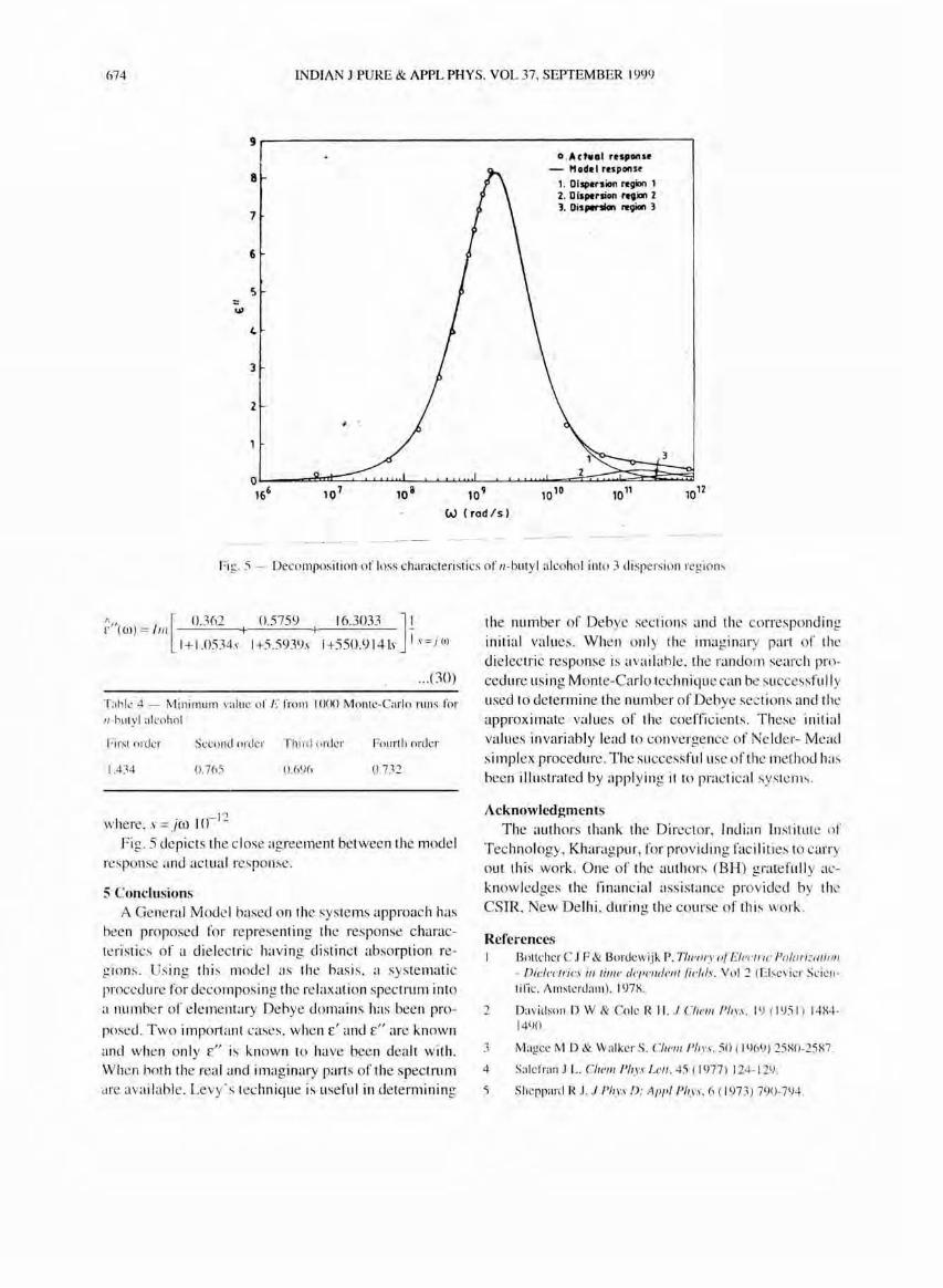
fi g . ."i - Decomposition of loss characteri sti cs o f II-butyl alcohol into 3 dispersion regions

f {J) = m + 1 -1\,,( ) I [ <U62 0.5759 16.3033] I

1+ 1.0534.1' 1+5.5939.1' 1+550.914h Is =) O)

... (30)

T;lhlc 4 - Minimuill value or I :' rroll! 1000 Monte-Carl o runs ror II-hutyl alcohol

First order Second order Th ird order Fourth order

1.434 0732

where, s =jw 10- 12

Fig. 5 depicts the c lose agreement between the mode l response and actual response .

5 Conclusions A General Model based on the systems approach has

been proposed fo r representing the response charac­teristics of a die lectri c having di stinct absorption re­g ions. Us ing thi s mode l as the basis , a systematic procedure for deco mpos ing the relaxation spectrum into a number of e le mentary De bye domains has been pro­

posed . Two important cases, when £' and £0 are known

and when only £0 is known to have been dealt with . Whe n both the real and imaginary parts of the spectrum are availabie. Levy's technique is useful in determining

the number of Debye sectio ns and the corresponding initial values. Whe n onl y the imaginary part of the dielectric response is ava il ab le. the random search pro­cedure using Monte-Carlo technique can be successfull y used to determine the number of Debye sec ti ons and the approximate values of the coefficients. These initi a l va lues invariably lead to convergence of Nelder- Mead

si mpl ex procedure. The successfu l use of the method has been illustrated by applying it to practical syste ms.

Acknowlcdgments The authors thank the Directo r, Indian In st itute of

Technology, Kharagpur, for providing faci I it ies to carry out (his work , One of the authors (BH) gratefull y ac­knowledges the financial assistance prov ided by the CSIR, New Delhi, during the course o f this work .

Rcfcl'cnccs I Bottcher C .I F & Bordewijk P. Th eory o/Electric Pol{/ri~{/t ioll

- Dielectrics ill tilJl e ticlIl'lulellt ./ieltls. Vol 2 (Ebevier Seiell ­Ii ri c. Amsterdam). 19711.

2 Davidson D W & Co le R I-I . .I Cllell! Pln·s. 19 ( 195 I ) 14114-14!)O.

3 Magee M D & Walker S. Cllelll Pin'.\' . 50 ( 1969) 25XO-25X7.

4 Salcl'ran J L . ChclII Pllys L"I/ , 45 ( 1977) 124- 129.

5 Shepparci R J . .1 PhI'S f): AJlII! PhI'S. 6 ( 1973) 790-794.

::..-

1

HEMALATH A l'1 ((I: DECOMPOSITION OF DIELECTRIC DISPERSION 675

6 Grosse C. J Mo/l'c Liq. 33 ( 19X6) 71-7R.

7 Hemalmha B. Frequellcy DOlllain Modelling ojLinear Dielec· Irics and Deve/oPIII('11I ()/ lechniques .fiJI' Idenlification (~/

Model Paramelers, Ph.D. thesis. 1997. liT Kharagpur. Inuia.

X Levy E C. IRE TrailS AlllOm COlllrol. 4 ( 1959) 37-43.

I) Press William H. Flannery Brinn P. Teukolsky Snul A & Yetterling William T . Nllmerical Recipe.~ in C. (Cnmbridge University Press. Oxford). 1988.

10 Grace Andy. Oplimization Toolhox For Use wilh MATLAB. Users's Guide. (The Math Works Inc. USA). 1996.

II MATLAB. Yersion4.2c. (The Math Work Inc. USA). 1996.

12 Garg S K & Smyth C P . .I Ph\'s Chelll . (1) (1986) 1294-130 , .

Appendix Levy's technique

The dielectric permitti vity, E*(S) can be represented in the Laplace domain as a transfer function:

p (s ) E * ( .1 ) = -- ... (1)

Q (.1)

where, pes) and Q(s) are polynomial s of the complex operator s.

P( ) 1 1.- 1 z (11 ) s = On + OIS + 0 2.1' + .. .. +0 /. . 1.1' + ({z.l· . . .

Q( .) - I I . 1 .2 I }I -I I ]I (Ill ) .1 - + )1.1 + 72.1 + .. ... + ) ,,_1.1 + )1" \ .. .

The roots of the denominator po lynomial give the transition frequencies and hence the relaxat ion times .

For phys ical systems p ~ :::. Si nce, dielectric systems

ha ve a finite E., and £.." the order of the numerator and denominator pol ynomial is same, that is p = ::: = n. Therefore

E, = an .. . (TV)

(f

... (V) E.C>'> =~ hll

If E':' (jOJ) is known over a wiele range of frequencies, the problem is to find the order of the numerator and the denominator polynomials and the corresponding coeffi ­cients which fit the data with a minimum error. In the frequency domain s =jOJ and E*(jOJ) ca n be written as:

. N? + iN I £* (.JOJ) = - . ...(VI ) D2 +jD I

where

N 1 5 1= (/ 1 OJ - (Il OJ + 0 , OJ + ...

:2 4 Nc = (to - {/ 2 OJ + (f~ OJ + ...

... (V II )

...(VlIl )

... (IX)

:2 . 4 D2 = I - b2 OJ + h4 CJ.) +.. . ...(X)

Therefore, the real and imaginary parts of E* (jOJ) are

E' ( OJ) = [Nl DI + N2 D?] D~+D~

E" ( CJ.) = (NI D~ + N: DI] DI+D"2

. ... (XI)

...(XII)

The error of fit at any specific frequency (0" is :

e( OJ" ) = ['E1 ( OJ" ) _ NI" D~" + N??" D? ,, ]

Dlk + D 2"

. ["(' ) N I" D?k +N?k Dl kJ .- .1 'E OJ" + ? 0

D1" + D 2" ... (X lII )

MUltiplying the above equation by D" (OJ,,) = DCIA +

D22k, and resolving into real and imaginary parts yields:

D\ OJk)e «(0,,) = A( OJ,,) - j B( OJ,,) . ..(XIV)

where , ??

A( OJ,,) = E ( OJ,, ) (D;A + D ; k ) - (N lk D I " + N2A D1k )

. .. (XV)

1/ 2 ~ B ( OJ,, ) = E (OJ,, ) (D " + D 2k ) + ( N ib D2" - N:'A DI A)

...( XVI)

By squaring the magnitude of the weighted error function, and summing it over the entire range of sam­pling frequencies, an objecti ve function} is obta ined as:

} = L.. ID" ( OJ. ) e ( OJ. ) I:'

A ~ I

M

"~ I

.. . (XVII )

Minimization oU with res pect to the unkn own pa-rameters would lead to an appropriat model repre­senting a good overall fit to the experi menta l data. Differentiating} with respect to each of the unk nown parameters and equating them to zero results in a set of linear simultaneous e(}u <1 ti ons, whose solution yields the va lues of the coe ffi cient s. S ince the system order is not known apri ori , the procedure is carri ed out for several assumed values of system order, and the oreler which corresponds to a minimum va lue of } is reckoned as the system order.