decomposition techniques for computational limit analysis
TRANSCRIPT

Universitat Politecnica deCatalunya
Departament de MatematicaAplicada III
Programa de Doctorat de MatematicaAplicada
Decomposition Techniques ForComputational Limit Analysis
Author:
Nima Rabiei
Supervisor:
Pro.Jose J.Munoz
PhD Thesis
Barcelona,September 22,
2014


ACKNOWLEDGEMENTS
This thesis becomes a reality with the kind support and help of many
individuals. I would like to extend my sincere thanks to all of them.
First of all, I would like to extend my special gratitude and thanks to my
supervisor, professor Jose J Munoz for tremendous support and
imparting his knowledge and expertise in this study.
I would like to express my deepest gratitude towards my beloved and
supportive wife, Bahar who is always by my side when times I needed her
most and helped me a lot in making this study. Also I would like to
express my gratitude to my supportive brother-in-law, Bijan Ebrahimi.
Deepest gratitude is also due to my parents for the encouragement and
endless love which helped me in completion of this thesis. Special thanks
also go to my sister and brothers who shared the burden with me.
I am highly in indebted to the Technical University of Catalonia,
department of Applied Mathematics III, the research group LaCaN
for giving me all facilities and work environment required for my study.
Finally, My thanks and appreciation also go to my colleagues Arjuna
Castrillon, Nina Asadipour and people who have willingly helped me out
with their abilities.
3


ABSTRACT
Limit analysis is relevant in many practical engineering areas such as
the design of mechanical structure or the analysis of soil mechanics. The
theory of limit analysis assumes a rigid, perfectly-plastic material to model
the collapse of a solid that is subjected to a static load distribution.
Within this context, the problem of limit analysis is to consider a contin-
uum that is subjected to a fixed force distribution consisting of both volume
and surfaces loads. Then the objective is to obtain the maximum multiple
of this force distribution that causes the collapse of the body. This multiple
is usually called collapse multiplier. This collapse multiplier can be obtained
analytically by solving an infinite dimensional nonlinear optimisation prob-
lem. Thus the computation of the multiplier requires two steps, the first
step is to discretise its corresponding analytical problem by the introduc-
tion of finite dimensional spaces and the second step is to solve a nonlinear
optimisation problem, which represents the major difficulty and challenge
in the numerical solution process.
Solving this optimisation problem, which may become very large and
computationally expensive in three dimensional problems, is the second im-
portant step. Recent techniques have allowed scientists to determine upper
and lower bounds of the load factor under which the structure will collapse.
Despite the attractiveness of these results, their application to practical ex-
amples is still hampered by the size of the resulting optimisation process.
Thus a remedy to this is the use of decomposition methods and to parallelise
5

6
the corresponding optimisation problem.
The aim of this work is to present a decomposition technique which can
reduce the memory requirements and computational cost of this type of
problems. For this purpose, we exploit the important feature of the un-
derlying optimisation problem: the objective function contains one scaler
variable λ. The main contributes of the thesis are, rewriting the constraints
of the problem as the intersection of appropriate sets, and proposing efficient
algorithmic strategies to iteratively solve the decomposition algorithm.

Contents
1. Introduction 15
1.1. Optimisation Problems in Limit Analysis . . . . . . . . . . . 16
1.1.1. Lower Bound Theorem . . . . . . . . . . . . . . . . . 19
1.1.2. Upper Bound Theorem . . . . . . . . . . . . . . . . . 19
1.1.3. Saddle Point Problem . . . . . . . . . . . . . . . . . 19
1.2. Lower Bound (LB) Problem . . . . . . . . . . . . . . . . . . 20
1.2.1. The Finite Element Triangulation . . . . . . . . . . . 20
1.2.2. Discrete Spaces for Lower Bound Problem . . . . . . 21
1.2.3. Implementation . . . . . . . . . . . . . . . . . . . . . 21
2. Cone Programs 27
2.1. Cone Programming Duality . . . . . . . . . . . . . . . . . . 28
2.2. Method of Averaged Alternating Reflection
(AAR Method) . . . . . . . . . . . . . . . . . . . . . . . . . 30
2.2.1. Best Approximation Operators . . . . . . . . . . . . 30
2.2.2. Nonexpansive Operators . . . . . . . . . . . . . . . . 32
2.2.3. Averaged Alternating Reflections (AAR) . . . . . . . 34
3. Decomposition Techniques 37
3.1. Introduction . . . . . . . . . . . . . . . . . . . . . . . . . . . 37
3.1.1. Complicating Constraints . . . . . . . . . . . . . . . 38
3.1.2. Complicating Variables . . . . . . . . . . . . . . . . . 40
3.2. Projected Subgradient Method . . . . . . . . . . . . . . . . . 41
7
8 Contents
3.3. Decomposition of Unconstrained Problems . . . . . . . . . . 41
3.3.1. Primal Decomposition . . . . . . . . . . . . . . . . . 41
3.3.2. Dual Decomposition . . . . . . . . . . . . . . . . . . 44
3.4. Decomposition with General Constraints . . . . . . . . . . . 46
3.4.1. Primal Decomposition . . . . . . . . . . . . . . . . . 46
3.4.2. Dual Decomposition . . . . . . . . . . . . . . . . . . 48
3.5. Decomposition with Linear Constraints . . . . . . . . . . . . 51
3.5.1. Splitting Primal and Dual Variables . . . . . . . . . . 51
3.5.2. Primal Decomposition . . . . . . . . . . . . . . . . . 51
3.5.3. Dual Decomposition . . . . . . . . . . . . . . . . . . 53
3.5.4. Benders Decomposition . . . . . . . . . . . . . . . . . 55
3.6. Simple Linear Example . . . . . . . . . . . . . . . . . . . . . 57
3.6.1. Primal Decomposition . . . . . . . . . . . . . . . . . 57
3.6.2. Dual Decomposition . . . . . . . . . . . . . . . . . . 58
3.6.3. Benders Decomposition . . . . . . . . . . . . . . . . . 60
3.7. Decomposition of Limit Analysis Optimisation Problem . . . 60
3.7.1. Decomposition of LB Problem . . . . . . . . . . . . . 61
3.7.2. Primal Decomposition (LB) . . . . . . . . . . . . . . 64
3.7.3. Dual Decomposition (LB) . . . . . . . . . . . . . . . 65
3.7.4. Benders Decomposition(LB) . . . . . . . . . . . . . . 66
4. AAR-Based Decomposition Algorithm 71
4.1. Alternative Definition of Global Feasibility Region . . . . . . 71
4.2. Definition of Subproblems . . . . . . . . . . . . . . . . . . . 74
4.3. Algorithmic Implementation of AAR-based Decomposition
Algorithm . . . . . . . . . . . . . . . . . . . . . . . . . . . . 78
4.3.1. Master Problem . . . . . . . . . . . . . . . . . . . . . 79
4.3.2. Subproblems . . . . . . . . . . . . . . . . . . . . . . 80
4.3.3. Justification of Update U2 for ∆k . . . . . . . . . . . 84
4.4. Mechanical Interpretation of AAR-based Decomposition Method 87
4.5. Numerical Results . . . . . . . . . . . . . . . . . . . . . . . . 89
4.5.1. Illustrative Example . . . . . . . . . . . . . . . . . . 89
4.5.2. Example 2 . . . . . . . . . . . . . . . . . . . . . . . . 91
5. Conclusions and Future Research 99
5.1. Conclusions . . . . . . . . . . . . . . . . . . . . . . . . . . . 99
5.2. Future Work . . . . . . . . . . . . . . . . . . . . . . . . . . . 101

Contents 9
A. Deduction of Lower Bound Discrete Problem 103
A.1. Equilibrium Constraint . . . . . . . . . . . . . . . . . . . . . 103
A.2. Inter-element Equilibrium Constraints . . . . . . . . . . . . 104
A.3. Boundary Element Equilibrium Constraints . . . . . . . . . 106
A.4. Membership Constraints . . . . . . . . . . . . . . . . . . . . 107
B. Background on Convex Sets 113
B.1. Sets in <n . . . . . . . . . . . . . . . . . . . . . . . . . . . . 113
B.2. The Extended Real Line . . . . . . . . . . . . . . . . . . . . 114
B.3. Convex Sets and Cones . . . . . . . . . . . . . . . . . . . . . 114
B.3.1. The Ice Cream Cone in <n(The Quadratic Cone) . . 115
B.3.2. The Rotated Quadratic Cone . . . . . . . . . . . . . 115
B.3.3. Polar and Dual Cones . . . . . . . . . . . . . . . . . 116
B.4. Farkas Lemma, Cone Version . . . . . . . . . . . . . . . . . 118
B.4.1. A Separation Theorem for Closed Convex Cones . . . 118
B.4.2. Adjoint Operators . . . . . . . . . . . . . . . . . . . 119
B.4.3. Farkas Lemma . . . . . . . . . . . . . . . . . . . . . . 121


List of Figures
1.1. Number of elements and corresponding number of degrees of
freedom (dof) in two- and three-dimensional analysis . . . . 17
1.2. Illustration of Neumann and Dirichlet parts of the domain Ω. 18
1.3. Scheme of the lower bound discrete spaces XLB and Y LB
used for the stresses and velocities, respectively. [37] . . . . . 21
2.1. Projection onto a nonempty closed convex set C in the Eu-
clidean plane. The characterization (2.2.2) states that p ∈C is the projection of x onto C if and only if the vectors
x − p and y − p form a right or obtuse angle for every
y ∈ C.([6],page 47) . . . . . . . . . . . . . . . . . . . . . . . 31
2.2. Illustration of reflection operator, RC = 2PC − I. . . . . . . 33
3.1. Convergence of global objective function using primal decom-
position for different rules of the step-size b. . . . . . . . . . 58
3.2. Convergence of global objective function using dual decom-
position for different rules of the step-size b. . . . . . . . . . 59
3.3. Dual decomposition using dynamic step size rule. . . . . . . 60
3.4. Evolution of upper and lower bound using Benders decompo-
sition. . . . . . . . . . . . . . . . . . . . . . . . . . . . . . . 61
3.5. Decomposition of global problem into two subproblems. The
global variables are the boundary traction t at the fictitious
Neumann condition and global load factor λ. . . . . . . . . 62
3.6. Benders decomposition, apply to the LB limit analysis problem. 70
11

12 List of Figures
4.1. Illustration of the iterative process . . . . . . . . . . . . . . 76
4.2. Illustration of the sets W (λ) and Z(λ) for the case λ ≤ λ∗
and λ > λ∗. . . . . . . . . . . . . . . . . . . . . . . . . . . . 78
4.3. Illustration of the sets W (λ) and Z(λ) on the (λ, t) plane. . 79
4.4. Updating parameter ∆k. (a): λk is considered as an upper
bound, (b): λk is considered as a lower bound. . . . . . . . . 83
4.5. Updating parameter ∆k, when λk is an upper bound. . . . . 86
4.6. Decomposition of global problem into two subproblems. The
global variables are the boundary traction t at the fictitious
Neumann condition and global load factor λ. . . . . . . . . 88
4.7. Evolution of λk for the toy problem. . . . . . . . . . . . . . . 92
4.8. (a) Evolution of λk for Problem 3, and (b) βn as a func-
tionofthe total numberof subiterations. . . . . . . . . . . . . 97
4.9. Evolution of the relative error for each master iteration. . . . 98
B.1. The ice cream cone [20] . . . . . . . . . . . . . . . . . . . . . 116
B.2. (a) A set C and its dual cone C∗, (b) A set C and its polar
cone C . . . . . . . . . . . . . . . . . . . . . . . . . . . . . 118
B.3. A point b not contained in a closed convex cone K ⊂ <2 can
be separated from K by a hyperplane h = x ∈ <2|y ·x = 0through the origin (left). The separating hyperplane resulting
from the proof of Theorem B.1(right). . . . . . . . . . . . . . 119

List of Tables
1.1. Number of elements and corresponding number of degrees of
freedom (dof) in two- and three-dimensional analysis. . . . . 17
3.1. Size and total master iterations of each problem solved using
SDPT3 [47]. . . . . . . . . . . . . . . . . . . . . . . . . . . . 69
4.1. Results of toy problem by using AAR-based decomposition
method. Number in bold font indicate upper bounds of λ∗. . 91
4.2. Size, CPU time and total subiterations of each problem solved
using Mosek [1] and SDPT3 [47]. . . . . . . . . . . . . . . . 93
4.3. Numerical results of Problem 1 . . . . . . . . . . . . . . . . 94
4.4. Numerical results of Problem 2 . . . . . . . . . . . . . . . . 94
4.5. Numerical results of Problem 3 . . . . . . . . . . . . . . . . 95
4.6. Numerical results of Problem 4 . . . . . . . . . . . . . . . . 95
4.7. Numerical results of Problem 5 . . . . . . . . . . . . . . . . 96
13


1Introduction
Limit analysis aims to directly determine the collapse load of a given
structural model without resorting to iterative and incremental analysis.
Computational techniques in limit analysis are based on the so-called limit
theorems, which are based on the minimization of the dissipation energy
and the maximization of the load factor, and they furnish lower and upper
bounds of the collapse load [14]. Assuming a rigid-perfectly plastic solid
subject to static load distribution, the problem of limit analysis consists in
finding the maximum multiple of this load distribution that will cause the
collapse of the body. As it will be explained in Section 1.1, the analytical
load factor results from solving an infinite dimensional saddle point problem,
where the internal work rate is minimized over the linear space of kinemat-
ically admissible velocities for which the external work rate equals unity.
Then load factor be also obtained by the maximum load over an admissible
set of stresses in equilibrium with the applied loads [33, 34, 37].
The aim of this work is to first present a general methodology to decom-
pose optimisation problems, and to apply this methodology to the optimi-
sation problems encountered in limit analysis.
The second part is to propose a decomposition technique which can al-
leviate the memory requirements and computational cost of this type of
problems.
This work has been motivated by the computational cost of the optimisa-
tion program in practical applications. It has been found that the memory
requirements and CPU time of the up-to-date available software to solve
optimisation problems, such as MOSEK[2], SDPT3[46], SeDuMi[45] or spe-
cific oriented software [32] are still not affordable if we want to analyse other
15

16 CHAPTER 1. INTRODUCTION
than academical problems. Then using decomposition methods seems an ap-
pealing technique for these analyses. For instance, Table 1.1 and Figure 1.1
show the number of elements and corresponding number of degrees of free-
dom (dof) for the lower bound (LB)1 and upper bound (UB) problem, in
two and three dimensions. As it can be observed, the number of dof in three
dimensions is always higher than in two dimensions for similar number of
elements, and becomes prohibitive for not so large meshes.
One of the possible solution is to parallelise the solution of the systems
of equations, which is inherent in all optimisation process. Although this
venue may alleviate the CPU time of the resolution process, the memory
requirements may still remain too large. For this reason, we propose to
partition ab initio the domain of the structure, and solve the optimisation
process in a decomposed manner. In doing this, there is no need to solve
nor to store the system of equations of the optimisation problem for the full
domain.
In this Chapter, we introduce limit analysis of structures and briefly de-
scribe discrete forms that give rise to the lower bound optimisation problem.
1.1. Optimisation Problems in Limit Analysis
Let Ω denote the domain of a body assumed to be made of a rigid-
perfectly plastic material, subjected to load volumetric load λf(gravity),
with λ an unknown load factor to be determined. Its boundary ∂Ω, consists
of a Neumann part ΓN and a Dirichlet part ΓD, which are such that ∂Ω =
ΓN ∪ ΓD and ΓN ∩ ΓD = ∅.The body velocities are equal to zero at the Dirichlet boundary, while the
Neumann boundary is subjected to the traction field λg, see Figure 1.2.
The objective of limit analysis is to compute the maximum value λ∗ of the
load factor at which the structure will collapse, and if possible, the velocity
1Discretisation of the problem in a particular fashion, i.e. combination of appro-priately selected interpolations for both the stresses and velocities results inestimating of the maximum multiple of the load factor that causes the collapseof the body, either from below or from above. The optimisation problem thatapproaches to the solution from below is so-called Lower Bound (LB) prob-lem and also the optimisation problem which approaches to the solution fromabove is called Upper Bound (UB) problem [34, 37].

CHAPTER 1. INTRODUCTION 17
2D 3D
# elements dof(LB) dof(UB) # elements dof(LB) dof(UB)
267 3309 4005 542 15719 25619
321 3989 4861 679 3433 2848
408 5097 6241 1144 32033 50597
598 7505 9265 3089 89582 154772
1723 21629 27205 4185 100441 95995
3110 39033 49369 8730 211672 360163
5644 70945 89897 24133 579193 565801
9283 84637 111665
24654 223588 296398
Table 1.1.: Number of elements and corresponding number of degrees of free-
dom (dof) in two- and three-dimensional analysis.
0 0.5 1 1.5 2 2.5
x 104
0
1
2
3
4
5
6x 10
5
Number of elements in two and three dimension space
dof
dof (LB) 2Ddof (UB) 2Ddof (LB) 3Ddof (UB) 3D
Figure 1.1.: Number of elements and corresponding number of degrees of
freedom (dof) in two- and three-dimensional analysis
field u∗ and tensor stress field σ∗, which allow us to identify the collapse
mechanism. The admissibility condition for the stress field is expressed by
the membership condition σ ∈ B, where the set B depends on the plastic

18 CHAPTER 1. INTRODUCTION
Figure 1.2.: Illustration of Neumann and Dirichlet parts of the domain Ω.
criteria adopted, and will be defined by the following general form:
B := σ|q(σ) ≤ 0.
The work rate of external loads associated with a velocity u = u(x) is
given by the following linear functional:
L(u) =
∫
Ω
f · u dΩ +
∫
ΓNg · u dΓ.
The velocity belongs to an appropriate space Y , to be specified in Sub-
section 1.1.1.
The work rate of the symmetric stress field σ associated with u is given
by the bilinear form:
a(σ,u) =
∫
Ω
σ : ε(u) dΩ +
∫
Γ
JuK · σn dΓ
=
∫
Ω
σ : ε(u) dΩ +
∫
Γ
JuK⊗n : σ dΓ,
where ε(u) = 12 [(∇u) + (∇u)T ], is the symmetric velocity gradient, and the
operator ⊗ is a symmetrized dyadic product: a⊗b = 12(a ⊗ b + b ⊗ a),
and Γ denotes the internal surface of domain Ω where the velocity field is
discontinuous. The symbol JuK, denotes the jump of field u on dΓ. The rate
of dissipated energy D(u) is defined as:
D(u) = supσ∈B
a(σ,u).
With these definitions at hand the upper and lower bound theorems may
be stated as follows:
CHAPTER 1. INTRODUCTION 19
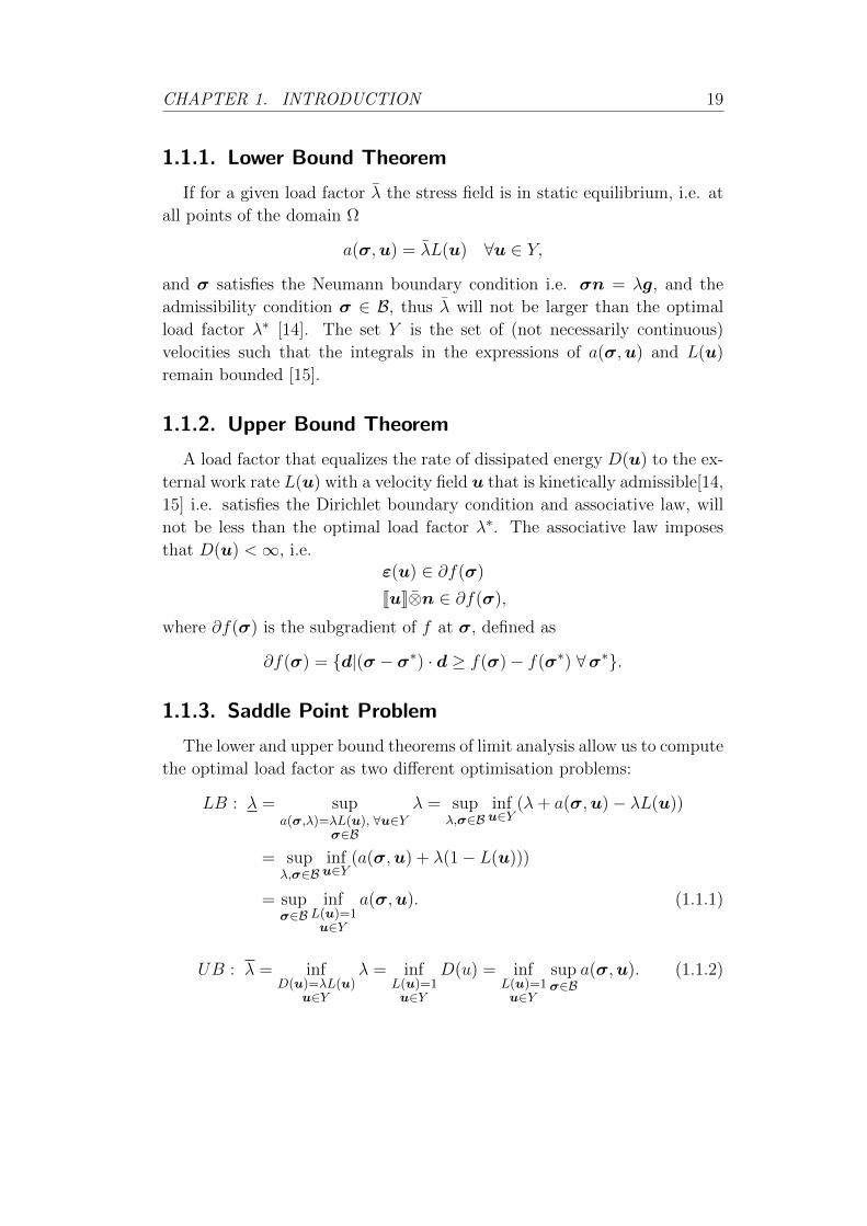
1.1.1. Lower Bound Theorem
If for a given load factor λ the stress field is in static equilibrium, i.e. at
all points of the domain Ω
a(σ,u) = λL(u) ∀u ∈ Y,
and σ satisfies the Neumann boundary condition i.e. σn = λg, and the
admissibility condition σ ∈ B, thus λ will not be larger than the optimal
load factor λ∗ [14]. The set Y is the set of (not necessarily continuous)
velocities such that the integrals in the expressions of a(σ,u) and L(u)
remain bounded [15].
1.1.2. Upper Bound Theorem
A load factor that equalizes the rate of dissipated energy D(u) to the ex-
ternal work rate L(u) with a velocity field u that is kinetically admissible[14,
15] i.e. satisfies the Dirichlet boundary condition and associative law, will
not be less than the optimal load factor λ∗. The associative law imposes
that D(u) <∞, i.e.ε(u) ∈ ∂f(σ)
JuK⊗n ∈ ∂f(σ),
where ∂f(σ) is the subgradient of f at σ, defined as
∂f(σ) = d|(σ − σ∗) · d ≥ f(σ)− f(σ∗) ∀σ∗.
1.1.3. Saddle Point Problem
The lower and upper bound theorems of limit analysis allow us to compute
the optimal load factor as two different optimisation problems:
LB : λ = supa(σ,λ)=λL(u), ∀u∈Y
σ∈B
λ = supλ,σ∈B
infu∈Y
(λ+ a(σ,u)− λL(u))
= supλ,σ∈B
infu∈Y
(a(σ,u) + λ(1− L(u)))
= supσ∈B
infL(u)=1u∈Y
a(σ,u). (1.1.1)
UB : λ = infD(u)=λL(u)
u∈Y
λ = infL(u)=1u∈Y
D(u) = infL(u)=1u∈Y
supσ∈B
a(σ,u). (1.1.2)

20 CHAPTER 1. INTRODUCTION
The comparison of the results in (1.1.1) and (1.1.2) shows that the UB
problem is the dual of the LB problem. Consequently, due to weak duality
we have:
λ = supσ∈B
infL(u)=1u∈Y
a(σ,u) ≤ infL(u)=1u∈Y
supσ∈B
a(σ,u) = λ.
If strong duality holds, the inequality above turns into equality. In this
case, we denote λ∗ = λ = λ = a(σ∗,u∗), where σ∗ and u∗ are the optimal
values of the stress and velocity field at the optimum. In addition, we can
obtain bounds of the optimum value λ∗ by evaluating the bilinear form
a(σ,u) at nonoptimal fields.
To be more specific, let us assume that the following optimisation problem
are computed exactly:
supσ∈B
a(σ,u) = a(σ∗,u), ∀u ∈ Y s.t L(u) = 1, (1.1.3)
infu∈YL(u)=1
a(σ,u) = a(σ,u∗), ∀σ ∈ B. (1.1.4)
In terms of equations (1.1.3) and (1.1.4) we have:
λ− = a(σ,u∗) ≤ a(σ∗,u∗) ≤ a(σ∗,u) = λ−, (1.1.5)
where σ is in static equilibrium and σ ∈ B, while L(u) = 1 and u satisfies
the associative law, that is, the fields σ and u are primal and dual feasible,
respectively.
1.2. Lower Bound (LB) Problem
1.2.1. The Finite Element Triangulation
When analysing the problem above in plane stress or plane strain, we will
consider the following triangular finite element discretisetion. Let τh denote
the triangulation, where h represent the typical size of the elements. The
mesh τh consists of ne (number of elements) triangular elements Ωe that
form a partition of the body, such that Ω = ∪nee=1Ωe, with all the element
being pairwise disjoint: Ωe ∩ Ωe′ = ∅ ∀ e, e′ ∈ τh. The boundary of the
element Ωe is denoted by ∂Ωe. Let ξ be the set of all the edges in the mesh,
which is decomposed into the following three disjoint sets: ξ = ξO ∪ ξD ∪ ξNwhere ξO, ξD and ξN are sets of interior edges, Dirichlet boundary and

CHAPTER 1. INTRODUCTION 21
Neumann boundary respectively. Mixed boundary, (edges with Dirichlet
and Neumann conditions), are not considered here, but the extension of the
problem statement to these situations dose not pose any further complexity.
1.2.2. Discrete Spaces for Lower Bound Problem
We will introduce a set of statically admissible spaces, that is, discrete
spaces σLB ∈ XLB and uLB ∈ Y LB that preserve the first inequality in
(1.1.5).
• XLB : Piecewise linear stress field interpolated from the nodal values
σi,e, i = 1, · · · , nn; e = 1, · · · , ne (nn is the number of nodes per ele-
ment, and ne the number of elements). Each element has a distinct set
of nodal values, and thus discontinuities at each elemental boundary
∂Ωe−e′(between element e and e′) are permitted.
• Y LB : constant velocity µe,LB at each element. Additionally, a linear
velocity field νξ,LB is introduced at each interior boundary ξO and
external boundary of ξN . We denote by uLB the complete set of
velocities, i.e. uLB = (µLB,νLB).
These spaces are depicted in Figure 1.3.
3.2 Lower bound (LB)
3.2.1 Statically admissible spaces
We will introduce a set of statically admissible spaces, that is, discrete spacesΣLB ∋ σLB and VLB ∋ µLB that preserve the first inequality in (23). Re-calling the derivations in (20), this is equivalent to satisfy the following in-equality:
supa(σLB ;µLB)=yℓ(µLB), ∀uLB∈VLB
σLB∈BLB
y ≤ supa(σ;µ)=yℓ(µ), ∀µ∈V
σ∈B
y (24)
This inequality is guaranteed if the following two conditions hold:
a) σ ∈ B ⇒ σLB ∈ BLB
b) a(σLB;µLB) = yℓ(µLB), ∀uLB ∈ VLB ⇒ a(σ;µ) = yℓ(µ), ∀µ ∈ V.
We will show that these conditions are indeed satisfied when resort-ing to the following interpolation spaces (see their representation in a two-dimensional case in Figure 1),
• ΣLB: Piecewise linear stress field interpolated from the nodal valuesσe,LB
i , i = 1, . . . , nn; e = 1, . . . , ne, with a set of complete Lagrangianfunctions I i, i.e.
∑nni Ii = 1 (nn is the number of nodes per ele-
ment, and ne the number of elements). Each element has a distinct setof nodal values, and thus discontinuities at each elemental boundary∂Ωe−e′ (between elements e and e′) are permitted.
• VLB: Constant velocity µe,LB at each element e. Additionally, a linearvelocity field νe−e′,LB is introduced at each interior boundary ∂Ωe−e′
and external boundary of ΓN .
µLB νLB
YLB :XLB :
σLB
(linear)
(constant)
+
(linear)
Figure 1: Interpolation spaces ΣLB and VLB.
In the plasticity criteria considered here, we will use a set BLB = B, withB convex, and impose the condition at the nodes, i.e. σLB ∈ B. Therefore,
17
Figure 1.3.: Scheme of the lower bound discrete spaces XLB and Y LB used
for the stresses and velocities, respectively. [37]
1.2.3. Implementation
The static equilibrium condition
a(σLB;uLB) = λL(uLB), ∀ uLB ∈ Y LB, (1.2.1)

22 CHAPTER 1. INTRODUCTION
is rewritten, after using the integration rules for discontinuous functions1:
a(σLB;µLB,νLB) = −∫
Ω
µLB · (∇ · σLB) dΩ
+∑
∂Ωξe′e
∫
∂Ωξe′e
νLB · JσKLB · n dΓ +
∫
ΓN
νLB · σLB · n dΓ,
L(µLB,νLB) =
∫
Ω
µLB · f dΩ +
∫
ΓN
νLB · g dΓ.
(1.2.2)
Consequently, due to the arbitrariness of the constant velocity µLB and
the linear velocity νLB the static equilibrium condition is equivalent to the
following equations:
∇ · σLB + λf = 0, in Ω
σLB · n = 0, in Γ
σLB · n = λg, in ΓN
σLB ∈ B.
(1.2.3)
The primal and dual LB problems may be obtained by inserting the
discrete space XLB and Y LB in primal optimisation problems and using
the bilinear and linear forms a(σLB,uLB) and L(uLB). In this case the
condition in (1.2.1), is equivalent to the following equations:
∇ · σe,LB + λf e = 0 in Ωe , ∀ e = 1, · · · , ne(σe,LB − σe′,LB) · nξe
′e = 0, ∀ ξe′e ∈ ξO
σe,LB · nξNe = λgξNe ∀ ξNe ∈ ξN
σe,LB ∈ B in Ωe, ∀ e = 1, · · · , ne
(1.2.4)
In Appendix A, it is shown that the equations in (1.2.4) may be trans-
formed into a set of linear constraints. The membership condition be also
rewritten, using a change of variable into a Lorentz cone membership. The
1We recall that whenever the product of functions fg is discontinuous, we havethat,
∫Ω(f ′g + g′f) =
∫∂Ω fg dΓ +
∑e−e′
∫∂Ωe−e′ JfgK dΓ, where the sum is
performed on all the boundaries where fg discontinuous.

CHAPTER 1. INTRODUCTION 23
resulting discrete optimisation problem is deduced in (A.4.9) and recast here:
λ∗LB = maxλ,x4,x1:3
λ
Aeq1P F 1 Aeq1P
Aeq2P 0 Aeq2P
Aeq3P F 3 Aeq3P
0 0 R
x4
λ
x1:3
=
0
0
0
b
,
x4 is free, λ ≥ 0, x1:3 ∈ K,|x4| = 3ne, |λ| = 1, |x1:3| = 9ne,
(1.2.5)
where
σ = Px4 + Qx1:3. (1.2.6)
The first, second, third and fourth rows of the matrix are respectively
the equilibrium constraints, inter-element equilibrium equations, boundary
Neumann conditions and the membership constraints given in (1.2.3). K is
the outer product of Lorentz cones Ln with n = 3, that is K = Ln1 × Ln2 ×· · · × Lnr . It follows that K is a convex cone. The matrices appearing in
(1.2.5) are explicitly deduced in Appendix A.
The size of the optimisation problem in (1.2.5) as it has been explained,
is proportional to the number of elements. If we want to obtain an accurate
value of λ∗LB, (i.e. value of λ∗LB that is close to λ∗), we must increase the
number of elements, which causes the increase of the size of the problem.
Since our sources like memory are limited, we are not able to increase the
number of elements as mush as we want to. Consequently, to solve larger
problem, we resort here to decomposition methods.
The development of general decomposition techniques has given rise to
numerous approaches, which include Benders decomposition [19, 26], prox-
imal point strategies [13], dual decomposition [10, 25], subgradient and
smoothing methods [38, 39], or block decomposition [36], among many oth-
ers. In the engineering literature, some common methods inherit either
decomposition methods for elliptic problems [29], or proximal point strate-
gies [30], or methods that couple the solutions from overlapping domains
[41], which reduce their applicability.
The accuracy of dual decomposition and subgradient techniques strongly
depend on the step-size control, while the accuracy of proximal point and
smoothing techniques depend on the regularisation and smoothing param-
eters, which are problem dependent and not always easy to choose. Also,

24 CHAPTER 1. INTRODUCTION
and from the experience of the authors, Benders methods have slow converge
rates in non-linear optimisation problems due to the outer-linearisation pro-
cess. These facts have motivated the development of the method presented
here, which is specially suited for nonlinear optimisation, and in particular
exploits the structure of the problems encountered in engineering applica-
tions. We aim to solve a convex optimisation problems that can be written
in the following form:
λ∗ = maxx1,x2,λ
λ
f1(x1, λ) = 0 (1.2.7a)
f2(x2, λ) = 0 (1.2.7b)
g1(x1) + g2(x2) = 0 (1.2.7c)
x1 ∈ K1 ⊆ <n1 , x2 ∈ K2 ⊆ <n2 , λ ∈ <, (1.2.7d)
where f1 : <n1 × < → <m1 ,f2 : <n2 × < → <m2 , g1 : <n1 → <m and
g2 : <n2 → <m are given affine functions, and K1, K2 are nonempty closed
convex sets.
The optimisation problem in (1.2.7) has one important feature, which is
a requirement of the method presented here: the objective function con-
tains one scalar variable λ. We remark though that other problems with
more complicated objectives may be also posed in the form given above,
and therefore may be also solved with the method proposed in this thesis.
We also point out that this particular form is a common feature in some
problems in engineering such as limit analysis [33, 35, 37] or general plastic
analysis [29, 30, 31], where λ measures the bearing capacity of a structure
or the dissipation power when it collapses. The primal problem in (1.2.7)
is written as a maximisation of the objective function, in agreement with
the engineering applications, but in contrast to the standard notation in
optimisation. We will keep the form in (1.2.7), but of course, the algorithm
explained in this thesis may be also described using standard notation.
The main contributions of the thesis are: (i) rewriting the constraints in
(1.2.7) as the intersection of appropriate sets, (ii) decomposing this form of
the algorithm into a master problem and two subproblems, (iii) applying
some results of proximal point theory to this new form of the optimisation
problem, and (iv) proposing efficient algorithmic strategies to iteratively
solve the decomposition algorithm. We prove the convergence properties of
the algorithm, and numerically test its efficiency.

CHAPTER 1. INTRODUCTION 25
The structure of the thesis is as follows. Some requisite background re-
sults are presented in Chapter 2. Chapter 3 describes some common method-
ologies to decompose general optimisation problems, and to particularise
them to the problems encountered in limit analysis, which have the struc-
ture of second order conic programming. Chapter 4 address the main con-
tributions and numerical results. Chapter 5 presents the main conclusions
and future work.


2Cone Programs
Here is the definition of a cone program, in a somewhat more general
format than we would need for our work. This will introduce symmetry
between the primal and the dual program.
Remark 2.1 Refer to Appendix B for definition of cone.
Definition 2.1 Let K ⊂ <n, L ⊂ <m be closed convex cones, b ∈ <m,
c ∈ <n, A : <n → <m a linear operator. A cone program is a constrained
optimisation problem of the form:
minxc · x
Ax− b ∈ Lx ∈ K.
(2.0.1)
For L = 0, we get cone programs in equality form.
Following the linear programming case, we call the cone program feasible
if there is some feasible solution, a vector x with Ax− b ∈ L, x ∈ K. The
value (optimal value) of a feasible cone program is defined as
infc · x : Ax− b ∈ L, x ∈ K, (2.0.2)
which includes the possibility that the value is +¯∞.
An optimal solution is a feasible solution x∗ such that c ·x∗ ≤ c ·x for all
feasible solutions x. Consequently, if there is an optimal solution, the value
of the cone program is finite, and that value is attained, meaning that the
infinitum (2.0.2) is a minimum.
27
28 CHAPTER 2. CONE PROGRAMS
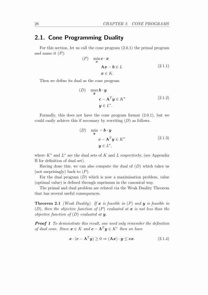
2.1. Cone Programming Duality
For this section, let us call the cone program (2.0.1) the primal program
and name it (P ):(P ) min
xc · x
Ax− b ∈ Lx ∈ K.
(2.1.1)
Then we define its dual as the cone program
(D) maxyb · y
c−ATy ∈ K∗
y ∈ L∗.(2.1.2)
Formally, this does not have the cone program format (2.0.1), but we
could easily achieve this if necessary by rewriting (D) as follows.
(D) miny− b · y
c−ATy ∈ K∗
y ∈ L∗,(2.1.3)
where K∗ and L∗ are the dual sets of K and L respectively, (see Appendix
B for definition of dual set).
Having done this, we can also compute the dual of (D) which takes us
(not surprisingly) back to (P ).
For the dual program (D) which is now a maximisation problem, value
(optimal value) is defined through suprimum in the canonical way.
The primal and dual problem are related via the Weak Duality Theorem
that has several useful consequences.
Theorem 2.1 (Weak Duality). If x is feasible in (P ) and y is feasible in
(D), then the objective function of (P ) evaluated at x is not less than the
objective function of (D) evaluated at y.
Proof 1 To demonstrate this result, one need only remember the definition
of dual cone. Since x ∈ K and c−ATy ∈ K∗ then we have
x · (c−ATy) ≥ 0⇒ (Ax) · y ≤ cx. (2.1.4)

CHAPTER 2. CONE PROGRAMS 29
On the other hand, since y ∈ L∗ and Ax− b ∈ L then
(Ax− b) · y ≥ 0⇒ b · y ≤ (Ax) · y, (2.1.5)
consequently, in view of (2.1.4) and (2.1.5) we have
b · y ≤ c · x.
One consequence is that any feasible solution of (D) provides a lower
bound on the optimal value of (P ); and any feasible solution of (P ) provides
an upper bound on the optimal value of (D). This can be useful in es-
tablishing termination or error control criteria when devising computational
algorithms addressed to (P ) and (D) ; if at some iteration feasible solutions
are available to both (P ) and (D) that are close to one another in value,
then they must be close to being optimal in their respective problems.
From Theorem 2.1, it also follows that (D) must be infeasible if the
optimal value of (P ) is −∞ and, similarly, (P ) must be infeasible if the
optimal value of (D) is +∞.
Definition 2.2 An interior point (or Slater point) of the cone program
(2.0.1) is a point x ∈ K with the property that
Ax− b ∈ int(L).
Let us remind the reader that int(L) is the set of all points of L that have
a small ball around it that is completely contained in L.
Theorem 2.2 (Strong Duality). If the primal program (P ) is feasible, has
finite optimal value γ, and has an interior feasible point x0, then the dual
program (D) is feasible and has finite optimal value β = γ.
Proof 2 See [27].
The strong Duality Theorem 2.2 is not applicable if the primal cone pro-
gram (P ) is in equality form (L = 0), since the cone L = 0 has no
interior points. But there is a different variant constraint qualification that
we can use in this case.

30 CHAPTER 2. CONE PROGRAMS
Theorem 2.3 If the primal program
(P ) minxc · x
Ax− b = 0
x ∈ K,
is feasible, has finite value γ and has a point x0 ∈ int(K) such that Ax0 = b,
the dual program
(D) maxyb · y
c−ATy ∈ K∗,
is feasible and has finite value β = γ.
Proof 3 See [27].
We remark that for general L, just requiring a point x0 ∈ int(K) with
Ax0 − b ∈ L is not enough to achieve strong duality.
In the next section, we consider the problem of finding a best approxima-
tion pair, i.e., two points which achieve the minimum distance between two
closed convex sets in <n. The method under consideration is termed AAR
for averaged alternating reflections and produces best approximation pairs
provided that they exist.
2.2. Method of Averaged Alternating Reflection
(AAR Method)
2.2.1. Best Approximation Operators
Definition 2.3 Let C be a subset of <n, let x ∈ <n, and let p ∈ C. Then
p is a best approximation to x from C (or a projection of x onto C) if
‖x− p‖ = dC(x) := inf‖z − x‖ : z ∈ C. (2.2.1)
If every point in <n has at least one projection onto C, then C is prox-
imal. If every point in <n has exactly one projection onto C, then C is a
Chebyshev set. In this case, the projector (or projection operator) onto C
is the operator, denoted by PC , that maps every point in <n to its unique
projection onto C.

CHAPTER 2. CONE PROGRAMS 31
Theorem 2.4 Let C be a nonempty closed convex subset of <n. Then C is
a Chebyshev set and, for every x and p in <n,
p = Pcx⇔ [p ∈ C and (∀y ∈ C), (x− p) · (y − p) ≤ 0]. (2.2.2)
Proof 4 See [24].
3.2 Best Approximation Properties 47
which establishes the characterization. ⊓⊔
•
•
•
C
x
y
p
Fig. 3.1 Projection onto a nonempty closed convex set C in the Euclidean plane. The
characterization (3.6) states that p ∈ C is the projection of x onto C if and only if thevectors x− p and y − p form a right or obtuse angle for every y ∈ C.
Remark 3.15 Theorem 3.14 states that every nonempty closed convex setis a Chebyshev set. Conversely, as seen above, a Chebyshev set must benonempty and closed. The famous Chebyshev problem asks whether everyChebyshev set must indeed be convex. The answer is affirmative if H is finite-dimensional (see Corollary 21.13), but remains an open problem otherwise.For a discussion, see [100].
The following example is obtained by checking (3.6) (further examples willbe provided in Chapter 28).
Example 3.16 Let C = B(0; 1). Then
(∀x ∈ H) PCx =1
max‖x‖, 1 x. (3.9)
Proposition 3.17 Let C be a nonempty closed convex subset of H, and letx and y be in H. Then Py+Cx = y + PC(x− y).Proof. It is clear that y+PC(x− y) ∈ y+C. Using Theorem 3.14, we obtain
(∀z ∈ C) 〈(y + z)− (y + PC(x− y)) | x− (y + PC(x− y)〉= 〈z − PC(x− y) | (x− y)− PC(x − y)〉≤ 0,
Figure 2.1.: Projection onto a nonempty closed convex set C in the Eu-
clidean plane. The characterization (2.2.2) states that p ∈ C is
the projection of x onto C if and only if the vectors x− p and
y−p form a right or obtuse angle for every y ∈ C.([6],page 47)
Remark 2.2 Theorem 2.4 states that every nonempty closed convex set is
a Chebyshev set.
Example 2.1 Let C = x : ‖x‖ ≤ 1. Then
(∀x ∈ <n) PCx =1
max‖x‖, 1x. (2.2.3)
A natural extension of the Definition 2.3 is to find a best approximation
pair relative to (C,W ) where C and W are subsets of <n. i.e., to
find (c, w) ∈ C ×W such that ‖c− w‖ = infc∈Cw∈W
‖c−w‖ := d(C,W ).
(2.2.4)

32 CHAPTER 2. CONE PROGRAMS
If W = w, (2.2.4) reduces to (2.2.1) and its solution is PCw. On the
other hand, when the problem is consistent, i.e., W ∩ C 6= ∅, then (2.2.4)
reduces to the well-known convex feasibility problem for two sets [5, 18] and
its solution set is (x,x) ∈ <n×<n|x ∈ W ∩C. The formulation in (2.2.4)
captures a wide range of problems in applied mathematics and engineering
[17, 28, 43].
2.2.2. Nonexpansive Operators
Nonexpansive operators play a central role in applied mathematics, be-
cause many problems in nonlinear analysis reduce to finding fixed points of
nonexpansive operators. In this section, we discuss nonexpansiveness and
several variants. The properties of the fixed point sets of nonexpansive op-
erators are investigated, in particular in terms of convexity.
Definition 2.4 Let D be a nonempty subset of <n and let T : D → <n.
Then T is
(i) firmly nonexpansive if
(∀x ∈ D), (∀y ∈ D) : ‖T (x)− T (y)‖2+‖(I − T )(x)− (I − T )(y)‖2
≤ ‖x− y‖2,
(ii) nonexpansive if
(∀x ∈ D), (∀y ∈ D) : ‖T (x)− T (y)‖ ≤ ‖x− y‖.
It is clear that firm nonexpansiveness implies nonexpansiveness.
Proposition 2.1 Let C be a nonempty closed convex subset of <n. Then
(i) the projector PC is firmly nonexpansive,
(ii) 2PC − I is nonexpansive.
See [6] for a proof of this lemma. The transformation 2PC − I is named
the reflection operator with respect to C and will be denoted by RC . See
Figure 2.2 for an illustration of the reflection operator .

CHAPTER 2. CONE PROGRAMS 33
Figure 2.2.: Illustration of reflection operator, RC = 2PC − I.
Definition 2.5 The set of fixed points of an operator T : X → X is denoted
by Fix T , i.e.,
Fix T = x ∈ X|T (x) = x. (2.2.5)
It is convenient to introduce the following sets, which we will use through-
out this section,
C = Z −W = z −w|z ∈ Z,w ∈ W,v = PC(0), G = W ∩ (Z − v), H = (W + v) ∩ Z,
(2.2.6)
where Z and W are nonempty closed convex subsets of <n and Z −Wdenotes the closure of Z −W . See Appendix B for a brief introduction to
convex sets.
Note also that if W ∩ Z 6= ∅, then G = H = W ∩ Z. However, even
when W ∩ Z = ∅, the sets G and H may be nonempty and they serve as
substitutes for the intersection. In words, vector v joins the two sets Z and
W at the point that are at the minimum distance and ‖v‖ measures the gap
between the sets W and Z.
Proposition 2.2 From the definitions in (2.2.5)-(2.2.6), the following iden-
tities hold:
(i) ‖v‖ = inf ‖W − Z‖.
(ii) G = Fix (PWPZ) and H = Fix (PZPW ).
(iii) G+ v = H.

34 CHAPTER 2. CONE PROGRAMS
The proof can be found in [4], Section 5.
Proposition 2.3 Suppose that (wn)n∈N and (zn)n∈N are sequences in W
and Z, respectively. Then
zn −wn → v ⇐⇒ ‖zn −wn‖ → ‖v‖.
Also, assume that zn −wn → v. Then the following identities hold:
(i) zn − PW (zn)→ v, and PZ(wn)−wn → v.
(ii) The weak cluster points of (wn)n∈N and (PW (zn))n∈N (resp.(zn)n∈Nand (PZ(wn))n∈N ) belong to G (resp.H). Consequently, the weak clus-
ter points of the sequences
((wn, zn))n∈N , ((wn), PZ(wn))n∈N ((PW (zn), zn)n∈N )
are best approximation pairs relative to (W,Z).
(iii) If G = ∅ or, equivalently, H = ∅, then
min‖wn‖, ‖zn‖, ‖PW (zn)‖, ‖PZ(wn)‖ → ∞.
These results are proved in [7].
Proposition 2.4 Let T1 : <n → <n and T2 : <n → <n be firmly nonexpan-
sive and set
T3 =(2T1 − I)(2T2 − I) + I
2.
Then the following results hold:
(i) T3 is firmly nonexpansive.
(ii) Fix T3 = Fix (2T1 − I)(2T2 − I).
2.2.3. Averaged Alternating Reflections (AAR)
Definition 2.6 We define the so-called Averaged Alternating Reflections
(AAR) operator, denoted by T and given by,
T =RWRZ + I
2, (2.2.7)

CHAPTER 2. CONE PROGRAMS 35
with RW and RZ the reflection operations illustrated in Figure 2.2.
Note that throughout this section, we assume thatW and Z are nonempty
closed convex subsets of <n.
In view of Proposition 2.1 and 2.4, and since RZ and RW are firmly
nonexpansive, we infer that T is firmly nonexpansive and
Fix T = Fix RWRZ .
Proposition 2.5 Let W and Z be nonempty closed convex subsets of <nand let T be the operator in (2.2.7). Then the following results hold:
(i) I − T = PZ − PWRZ .
(ii) W ∩ Z 6= ∅ if and only if Fix T 6= ∅.
Proof 5 (i):
T =RWRZ + I
2=
2PWRZ −RZ + I
2=
2PWRZ − 2PZ + I + I
2= PWRZ − PZ + I ⇒ I − T = PZ − PWRZ .
(ii): Assume that x ∈ W ∩ Z. Clearly, we then have that PW (x) = x and
PZ(x) = x, which in turn imply that RW (x) = x and RZ(x) = x. Using
the definition in (2.2.7), it follows that
T (x) = x,
so that Fix T 6= ∅.Conversely, if x ∈ Fix T , then T (x) = x, and then according to (i), we
have, that PZ(x) = PWRZ(x), and therefore PZ(x) ∈ Z and PZ(x) ∈ W ,
which is equivalent to PZ(x) ∈ W ∩ Z.
We now recall the well known convergence results for the method of Av-
eraged Alternating Reflections (AAR).
Proposition 2.6 (Convergence of AAR method). Consider the following
successive approximation method: Take t0 ∈ <n, and set
tn = Tn(t0) = T (tn−1), n = 1, 2, . . .
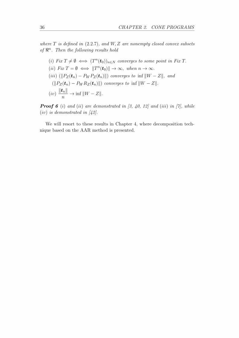
36 CHAPTER 2. CONE PROGRAMS
where T is defined in (2.2.7), and W,Z are nonempty closed convex subsets
of <n. Then the following results hold
(i) Fix T 6= ∅ ⇐⇒ (Tn(t0))n∈N converges to some point in Fix T.
(ii) Fix T = ∅ ⇐⇒ ‖Tn(t0)‖ → ∞, when n→∞.(iii) (‖PZ(tn)− PWPZ(tn)‖) converges to inf ‖W − Z‖, and
(‖PZ(tn)− PWRZ(tn)‖) converges to inf ‖W − Z‖.
(iv)‖tn‖n→ inf ‖W − Z‖.
Proof 6 (i) and (ii) are demonstrated in [3, 40, 12] and (iii) in [7], while
(iv) is demonstrated in [42].
We will resort to these results in Chapter 4, where decomposition tech-
nique based on the AAR method is presented.

3Decomposition Techniques
3.1. Introduction
The size of an optimisation problem can be very large and it is not hard to
encounter practical problems with several hundred thousands of equations or
unknowns (see Table 1.1). In order to solve such problems, it is convenient
to design some special techniques. Decomposition is a general approach to
solving a problem by breaking it up into smaller ones and solving each of
the smaller ones separately, either in parallel or sequentially in conjunction
with a master problem that couples the subproblems. (When it is done
sequentially, the advantage comes from the fact that problem complexity
grows more than linearly). Decomposition in optimisation is an old idea,
and appears in the early works on large-scale linear problems (LPs) in the
1960s [23]. A good reference on decomposition methods is Chapter 6 of
Bertsekas [9]. The original primary motivation for decomposition methods
was to solve very large problems that where beyond the reach of standard
techniques, possibly using multiple processors.
The idea of decomposition comes up in the context of solving linear equa-
tions, but goes by other names such as block elimination, Schur complement
methods, or (for special cases) matrix inversion lemma (see [11]). The core
idea, i.e., using efficient methods to solve subproblems, and combining the
results in such a way as to solve the larger problem, is the same as the one
exploited here when decomposing an optimisation problem, although the
techniques are slightly different.
The original primary motivation for decomposition methods was to solve
very large problems that were beyond the reach of standard techniques,
37

38 CHAPTER 3. DECOMPOSITION TECHNIQUES
possibly using multiple processors [23, 8]. This remains a good reason to use
decomposition methods for some problems. But other reasons are emerging
as equally (or more) important. In many cases decomposition methods
yield decentralized solution methods. Even if the resulting algorithms are
slower (in some cases, much slower) than centralized methods, decentralized
solutions might be prefered for other reasons. For example, decentralized
solution methods can often be translated into, or interpreted as, simple
protocols that allow a collection of subsystems to coordinate their actions
to achieve global optimality [44].
Problems for which the variables can be decomposed into uncoupled sets
of equations are called separable. As a general example of such a problem,
suppose that variable x can be partitioned into subvectors x1,x2, · · · ,xk,the cost function is a sum of functions of xi, and each constraint only involves
the local subvectors xi. Then, evidently we can solve each problem involving
xi separately, and re-assemble the solutions into x.
A more interesting situation occurs when there is some coupling or inter-
action between the subvectors, so the problems cannot be solved indepen-
dently. For these cases there are techniques that solve the overall problem
by iteratively solving a sequence of smaller problems. There are many ways
to do this. In this Chapter we review some well-known decomposition tech-
niques [19, 8, 23] and illustrate their efficiency with some simple examples
and some problems in limit analysis. These results will motivate the pro-
posed method in Chapter 4.
The efficiency and applicable of a decomposition technique depends on
the structure of the problem at hand. Two basic structures arise in prac-
tice, problems with complicating constraints and problems with complicat-
ing variables structures to be described next.
3.1.1. Complicating Constraints
Let us assume a linear optimisation problem where the primal variables
have been partitioned into different blocks. Complicating constraints involve
variables from different blocks, which drastically complicate the solution of
the problem and prevent its solution by blocks. The following example illus-
trates how complicating constraints impede a solution by blocks. Consider

CHAPTER 3. DECOMPOSITION TECHNIQUES 39
the problem:
minxi,yi
a1x1 +a2x2 +a3x3 +b1y1 +b2y2
a11x1 +a12x2 +a13x3 = e1
a21x1 +a22x2 +a23x3 = e2
b11y1 +b12y2 = g1
b21y1 +b22y2 = g2
d11x1 +d12x2 +d13x3 +d14y1 +d15y2 = h1
x1 ≥ 0, x2 ≥ 0, x3 ≥ 0, y1 ≥ 0, y2 ≥ 0.
(3.1.1)
If the last equality is not enforced, i.e., it is relaxed, the above problem
decomposes into the following two subproblems:
Subproblem 1:
minx1,x2,x3
a1x1 + a2x2 + a3x3
a11x1 + a12x2 + a13x3 = e1
a21x1 + a22x2 + a23x3 = e2
x1 ≥ 0, x2 ≥ 0, x3 ≥ 0
Subproblem 2:
miny1,y2
b1y1 + b2y2
b11y1 + b12y2 = g1
b21y1 + b22y2 = g2
y1 ≥ 0, y2 ≥ 0
Since the last equality constraint in (3.1.1) involves all variables, prevent-
ing a solution by blocks, this equation is a complicating constraint.
Decomposition procedures are computational techniques that indirectly
consider the complicating constraints and solve a set of problems with smaller
size. The price that has to be paid for such a size reduction is the amount
of subproblems to be solved. In other words, instead of solving the original
problem with complicating constraints, two problems are solved iteratively:
a simple so-called master problem, and a set of subproblems, similar to those
included in the original one but without complicating constraints.

40 CHAPTER 3. DECOMPOSITION TECHNIQUES
3.1.2. Complicating Variables
In linear problems, the complicating variables are those variables prevent-
ing a solution of the problem by independent blocks. For instance, let us
consider the following problem:
minxi,yi,λ
a1x1 +a2x2 +a3x3 +b1y1 +b2y2
a11x1 +a12x2 +a13x3 +d11λ = e1
a21x1 +a22x2 +a23x3 +d21λ = e2
b11y1 +b12y2 +d31λ = g1
b21y1 +b22y2 +d41λ = g2
x1 ≥ 0, x2 ≥ 0, x3 ≥ 0, y1 ≥ 0, y2 ≥ 0, λ ≥ 0
If variable λ is given the fixed value λfixed ≥ 0 the problem decomposes
into the two subproblems:
Subproblem 1:
miny1,y2
a1x1 + a2x2 + a3x3
a11x1 + a12x2 + a13x3 = e1 − d11λfixed
a21x1 + a22x2 + a23x3 = e2 − d21λfixed
x1 ≥ 0, x2 ≥ 0, x3 ≥ 0.
Subproblem 2:
miny1,y2
b1y1 + b2y2
b11y1 + b12y2 = g1 − d31λfixed
b21y1 + b22y2 = g2 − d41λfixed
y1 ≥ 0, y2 ≥ 0.
In the subsequent sections we will describe some decomposition methods:
primal decomposition, dual decomposition, and Benders decomposition. We
apply these techniques to some illustrative toy problems.
Before, we introduce an iterative method for solving optimisation prob-
lems called projected subgradient method. This method will be employed
in the reminder of the present Chapter.

CHAPTER 3. DECOMPOSITION TECHNIQUES 41
3.2. Projected Subgradient Method
We aim to solve the following constrained optimisation problem:
minxf(x)
x ∈ C,where f : Rn → R, and C ⊆ Rn are convex. The projected subgradient
method consists on given a feasible candidate xk, obtain a feasible next
iterate xk+1 as,
xk+1 = P(xk − αkgk), (3.2.1)
where P is an operator that projects its argument on C, and gk ∈ ∂f(xk),
with ∂f(xk) the set of all subgradients of function f at point xk. For
instance if C is the set of linear equality constraints, that is C = x|Ax =
b, then the projection of z onto C reads,
P(z) = z −AT (AAT )−1(Az − b)= (I−AT (AAT )−1A)z + AT (AAT )−1b.
(3.2.2)
In this case, after using Axk = b, the update process in (3.2.1) yields,
xk+1 = P(xk − αkgk)= xk − αk(I−AT (AAT )−1A)gk,
where αk is a step size. There are some rules for choosing appropriately αkwhich will be considered below.
Note that if P is the identity projection, then the method turns into the
subgradient method, which does not enforce the feasibility of xk+1.
3.3. Decomposition of Unconstrained Problems
3.3.1. Primal Decomposition
We will consider the simplest possible case, an unconstrained optimisa-
tion problem that splits into two subproblems. (But note that the most
impressive applications of decomposition occur when the problem is split
into many subproblems.) In our first example, we consider an unconstrained
minimization problem, of the form :
minxf(x) = min
x1,x2,yf1(x1,y) + f2(x2,y) (3.3.1)

42 CHAPTER 3. DECOMPOSITION TECHNIQUES
where the variable is x = (x1,x2,y). Although the dimensions do not
matter here, it is useful to think of x1 and x2 as having relatively high
dimension, and y having relatively small dimension. The objective is almost
block separable in x1 and x2; indeed, if we fix the subvector y, the problem
becomes separable in x1 and x2, and therefore can be solved by solving the
two subproblems independently. For this reason, y is called the complicating
variable, because when it is fixed, the problem splits or decomposes. In
other words, the variable y complicates the problem. It is the variable that
couples the two subproblems. We can think of x1(x2) as the private variable
or local variable associated with the first (second) subproblem, and y as the
public variable or interface variable or boundary variable between the two
subproblems. Indeed, by rewriting (3.3.1) as:
miny
(minx1
f1(x1,y) + minx2
f2(x2,y)
), (3.3.2)
we observe that the problem becomes separable when y is fixed. This sug-
gests a method for solving the problem (3.3.1). Let gi(y) denote the inner
optimum in the previous expression,
gi(y) = minxi
fi(xi,y) (i = 1, 2). (3.3.3)
Note that if f1 and f2 are convex, so are g1 and g2. We refer to (3.3.3)
as subproblem(i), (i = 1, 2).
Then the original problem in (3.3.1) is equivalent to the following master
problem:
minyg1(y) + g2(y).
If the original problem is convex, so is the master problem. The variables
of the master problem are the complicating or coupling variables of the
original problem. The objective of the master problem is the sum of the
optimal values of the subproblems.
A decomposition method solves the problem (3.3.1) by solving the mas-
ter problem, using an iterative method such as the subgradient method de-
scribed in Section 3.2. Each iteration requires solving the two subproblems
in order to evaluate g1(y) and g2(y) and their gradients and subgradients.
This can be done in parallel, but even if it is done sequentially, there will be

CHAPTER 3. DECOMPOSITION TECHNIQUES 43
substantial savings if the computational complexity of the problems grows
more than linearly with problem size.
Lets see how to evaluate a subgradient of g1 at y, assuming the problem
is convex. We first solve the associated subproblem, i.e., we find x1(y) that
minimizes f1(x1,y). Thus, there is a subgradient of f1 of the form (0, q1),
and not surprisingly, q1 is a subgradient of g1 at y. We can carry out
the same procedure to find a subgradient q2 ∈ ∂g2(y). Then q1 + q2 is a
subgradient of g1 + g2 at y.
We can solve the master problem by a variety of methods, including
subgradient method (if the functions are nondifferentiable). This basic de-
composition method is called primal decomposition because the master al-
gorithm manipulates (some of the) primal variables.
When we use a subgradient method to solve the master problem, we
obtain the following primal decomposition algorithm:
Repeat
• Solve the subproblems in (3.3.3), possibly in parallel. Set y = yk.
– Find x1 that minimizes f1(x1,yk), and a subgradient q1 ∈ ∂g1(yk).
– Find x2 that minimizes f2(x2,yk), and a subgradient q2 ∈ ∂g2(yk).
• Update complicating variable,
yk+1 = yk − αk(qk1 + qk2).
Here αk is a step length that can be chosen in any of the standard
ways [9].
When a subgradient method is used for the master problem, and both g1
and g2 are differentiable, the update has a very simple interpretation. We
interpret q1 and q2 as the gradients of the optimal value of the subproblems,
with respect to the complicating variable y. The update simply moves the
complicating variable in a direction of improvement of the overall objective.
The basic primal decomposition method described above can be extended
in several ways. We can add separable constraints, i.e., constraints of the
form x1 ∈ C1 and x2 ∈ C2. In this case (and also, in the case when domfiis not all vectors) we have the possibility that gi(y) = ∞ (i.e., y /∈ domgi)
for some choices of y. In this case we find a cutting-plane that separates y
from dom gi, to use in the master algorithm.

44 CHAPTER 3. DECOMPOSITION TECHNIQUES
3.3.2. Dual Decomposition
We can apply decomposition to the problem (3.3.1) after introducing
some new variables, and working with the dual problem. We first rewrite
the problem as
minx1,x2,y
f1(x1,x2,y) + f2(x1,x2,y) = minx1,x2,y1=y2
f1(x1,y1) + f2(x2,y2)
We have introduced a local version of the complicating variable y, along
with a consistency constraint that requires the two local versions to be equal.
Note that the objective is now separable, with the variable partition (x1,y1)
and (x2,y2). Now we form the dual problem. The Lagrangian is equal to:
L(x1,y1,x2,y2,v) = f1(x1,y1) + f2(x2,y2) + v · (y1 − y2)
= f1(x1,y1) + f2(x2,y2) + v · y1 − v · y2,
which is separable. The dual function is given by
q(v) = q1(v) + q2(v),
where
q1(v) = infx1,y1
f1(x1,y1) + v · y1,
q2(v) = infx2,y2
f2(x2,y2)− v · y2.(3.3.4)
Note that q1 and q2 can be evaluated completely independently, e.g, in
parallel. The dual problem reads:
maxv
q1(v) + q2(v), (3.3.5)
with the dual variable v. This is the master problem in dual decomposition.
The master algorithm solve this problem using a subgradient method or
other methods.
To evaluate a subgradient of −q1 or −q2 is easy. We find x1 and y1 that
minimize f1(x1,y1)+v ·y1 over x1 and y1. Then a subgradient of −q1 at v
is given by −y1. Similarly, if x2 and y2 minimize f2(x2,y2)−v ·y2 over x2
and y2 , then a subgradient of −q2 at v is given by y2. Thus, a subgradient
of the negative dual function −q is given by y2− y1, which is nothing more
than the consistency constraint residual.
If we use a subgradient method to solve the master problem, the dual
decomposition algorithm has the following form:
Repeat
CHAPTER 3. DECOMPOSITION TECHNIQUES 45
• Solve the subproblems in (3.3.4), possibly in parallel. Set v = vk.
– Find xk1 and yk1 that minimize f1(x1,y1) + vk · y1.
– Find xk2 and yk2 that minimize f2(x2,y2)− vk · y2.
• Update dual variables.
vk+1 = vk + βk(yk1 − yk2).
Here βk is a step size which can be chosen in several ways.
If the dual function q is differentiable, then we can choose a constant step
size, provided it is small enough. Another choice in this case is to carry out
a line search on the dual objective. If the dual function is nondifferentiable,
we can use a diminishing nonsummable step size, such as βk = αk [8], which
satisfies the following properties.
limk→∞
βk = 0,
∞∑
k=1
βk =∞.
At each step of the dual decomposition algorithm, we have a lower bound
on P ∗, the optimal value of the original problem, given by
P ∗ ≥ q(v) = f1(x1,y1) + v · y1 + f2(x2,y2)− v · y2,
where x1, y1, x2 and y2 are the iterates. Generally, the iterates are not
feasible for the original problem, i.e., we have y2 − y1 6= 0. (If they are
feasible, we have maximized q.) A reasonable guess of a feasible point can be
constructed from this iterate as (x1, y), (x2, y), where y =(y1+y2)
2 . In other
words, we replace y1 and y2 (which are different) with their average value.
(The average is the projection of (y1,y2) onto the feasible set y1 = y2).
This gives an upper bound on P ∗, given by P ∗ ≤ f1(x1, y) + f2(x2, y).
A better feasible point can be found by replacing y1 and y2 with their
average, and then solving the two subproblems (3.3.3) encountered in primal
decomposition, i.e., by evaluating g1(y) + g2(y). This gives the bound
P ∗ ≤ g1(y) + g2(y).
There is one subtlety in dual decomposition. Even if we do find the
optimal dual solution v∗, there is the question of finding the optimal values

46 CHAPTER 3. DECOMPOSITION TECHNIQUES
of x1, x2, and y. When f1 and f2 are strictly convex, the points found in
evaluating q1 and g2 are guaranteed to converge to optimal, but in general
the situation can be more difficult. (For more on finding the primal solution
from the dual, see ([11], section 5.5.5).
As in the primal decomposition method, we can encounter infinite values
for the subproblems. In dual decomposition, we can have qi(v) = ∞. This
can occur for some values of v, if the functions fi grow only linearly in yi. In
this case we generate a cutting-plane that separates the current price vector
from domgi(y), and use this cutting-plane to update the price vector.
3.4. Decomposition with General Constraints
Up to now, we have considered the case where two problems are separable,
except for some complicating variables that appear in both problems. We
can also consider the case where the two subproblem are coupled through
constraints that involve both set of variables. As a simple example, suppose
our problem has the form :
min f1(x1) + f2(x2)
x1 ∈ C1, x2 ∈ C2
h1(x1) + h2(x2) ≤ 0.
(3.4.1)
Here C1 and C2 are feasible sets of the subproblems. The function h1 :
<n → <p and h2 : <n → <p have components that are convex. The
subproblems are coupled through p constraints that involve both x1 and
x2. We refer to these as complicating constrains (since without them, the
problem involving x1 and x2 can be solved separately).
3.4.1. Primal Decomposition
To use primal decomposition, we can introduce a variable t ∈ <p that
represent the amount of the resources allocated to the first subproblem. As
a result, −t is allocated to the second subproblem. Then subproblems are,
minxifi(xi)
hi(xi) ≤ (−1)i+1t (i = 1, 2),
xi ∈ Ci.(3.4.2)

CHAPTER 3. DECOMPOSITION TECHNIQUES 47
Let gi(t) denote the optimal value of the subproblem (3.4.2). Evidently
the original problem (3.4.1) is equivalent to the master problem of
mintg(t) = g1(t) + g2(t),
over the allocation vector t. Subproblems in (3.4.2) can be solved separately,
when t is fixed.
We can find a subgradient for the optimal value of each subproblem from
an optimal dual variable associated with the coupling constraints. Let p(z)
be the optimal value of the convex optimisation problem
p(z) = minx
f(x)
h(x) ≤ zx ∈ X, (X is a closed convex set),
and suppose z ∈dom(p). Let µ be an optimal dual variable associated with
the constraint h(x) ≤ z. Then, −µ is a subgradient of p(z) at z. To see
this, we consider the value of p at an arbitrary point z such that z ∈dom(p):
p(z) = maxµ≥0
minx∈X
(f(x) + µ · (h(x)− z))
≥ minx∈X
(f(x) + µ · (h(x)− z))
= minx∈X
(f(x) + µ · (h(x)− z − z + z))
= minx∈X
(f(x) + µ · (h(x)− z)) + µ · (z − z)
= p(z) + (−µ) · (z − z).
It follows that −µ is a subgradient of p at z (see[8]). Consequently, in
order to find a subgradient of g, we solve the two subproblems, we find the
optimal vectors x1 and x2, as well as the optimal dual variables µ1 and µ2,
associated with the constraints h1(x1) ≤ t and h2(x2) ≤ −t, respectively.
Then we have that µ2 − µ1 ∈ ∂g(t). It is also possible that t /∈ dom(g). In
this case we can generate a cutting plane that separates t from dom(g), for
use in the master algorithm.
Primal decomposition, using a subgradient method algorithm, can be
achieved following the next steps:
Repeat
• Solve the subproblems in (3.4.2), possibly in parallel.

48 CHAPTER 3. DECOMPOSITION TECHNIQUES
– Find an optimal x1 and µk1.
– Find an optimal x2 and µk2.
• Update resource allocation,
tk+1 = tk − αk(µk2 − µk1).
with αk an appropriate step size. At every step of this algorithm we
have points that are feasible for the original problem.
3.4.2. Dual Decomposition
Dual decomposition for this example is straightforward. We form the
partial Lagrangian,
L(x1,x2;µ) = f1(x1) + f2(x2) + µ · (h1(x1) + h2(x2))
= (f1(x1) + µ · h1(x1)) + (f2(x2) + µ · h2(x2)),
which is separable for a some µ, so we can minimize over x1 and x2 sepa-
rately, given the dual variable µ to find q(µ) = q1(µ) + q2(µ). For example,
to find qi(µ); (i = 1, 2), we solve the subproblem
qi(µ) = min fi(xi) + µ · hi(xi)xi ∈ Ci.
(3.4.3)
A subgradient of q at µ is h1(x1) + h2(x2), where x1 and x2 are any
solutions of subproblems. The master algorithm updates µ based on this
subgradient.
If we use a projected subgradient method to update µ we get a very
simple algorithm.
Repeat
• Solve the subproblems in (3.4.3), possibly in parallel.
– Find an optimal xk1
– Find an optimal xk2
• Update dual variables:
µk+1 = (µk + βk(h1(xk1) + h2(xk2)))+.

CHAPTER 3. DECOMPOSITION TECHNIQUES 49
At each step we have a lower bound on P ∗, given by
q(µ) = q1(µ) + q2(µ) = f1(x1) + f2(x2) + µ · (h1(x1) + h2(x2)).
The iterates in the dual decomposition method need not be feasible, i.e.,
we can have h1(x1) + h2(x2) ≤ 0. At the cost of solving two additional
subproblems, however, we can (often) construct a feasible set of variables,
which will give us an upper bound on P ∗. When h1(x1) + h2(x2) 0, we
define
t =h1(x1)− h2(x2)
2, (3.4.4)
and solve the primal subproblems (3.4.2). As in primal decomposition, it
can happen that t /∈ domg. But when t ∈ domg, this method gives a feasible
point, and an upper bound on P ∗.
Note that for the dual problem we can find a subgradient as follows.
Consider the following optimisation problem in general:
minx
f(x)
g(x) ≤ 0
h(x) = 0
x ∈ X, X is a nonempty set.
Its dual problem is given by,
maxµ,λ
q(µ,λ)
µ ≥ 0,λ free,
where q(µ,λ) is defined as follows:
q(µ,λ) = minx∈X
L(x;µ,λ)
with
L(x;µ, λ) = f(x) + µ · g(x) + λ · h(x) = f(x) +
µ
λ
·g(x)
h(x)
.
Assume that for (µ, λ), some vector x minimizes L(x, µ, λ) over X that
is:
q(µ, λ) = minx∈X
L(x; µ, λ) = f(x) +
µ
λ
·g(x)
h(x)
,
50 CHAPTER 3. DECOMPOSITION TECHNIQUES
then we have:
q(µ,λ) ≤ f(x) +
µ
λ
·g(x)
h(x)
= f(x) +
µ
λ
·g(x)
h(x)
+
µ
λ
·g(x)
h(x)
−µ
λ
·g(x)
h(x)
= q(µ, λ) +
g(x
h(x
· (µ
λ
−µ
λ
).
It means that: g(x)
h(x)
∈ ∂q(µ, λ).
Except for the details of computing the relevant subgradients, primal
and dual decomposition for problems with coupling variables and coupling
constraints seem quite similar. In fact, we can readily transform each into the
other. For example, we can start with the problem with coupling constraints
(3.4.1), and introduce new variables y1 and y2, that bound the subsystem
coupling constraint functions, to obtain
minx1,y1,x2,y2
f1(x1) + f2(x2)
h1(x1) ≤ y1
h2(x2) ≤ y2
y1 + y2 = 0
x1 ∈ C1, x2 ∈ C2.
(3.4.5)
We now have a problem that is separable, except for a consistency con-
straint, that requires two (vector) variables of the subproblems to be equal.
Any problem that can be decomposed into two subproblems that are
coupled by some common variables, or equality or inequality constraints,
can be put in this standard form, i.e., two subproblems that are independent
except for one consistency constraint, that requires a subvariable of one to
be equal to a subvariable of the other. Primal or dual decomposition is then
readily applied; only the details of computing the needed subgradients for
the master problem vary from problem to problem.

CHAPTER 3. DECOMPOSITION TECHNIQUES 51
3.5. Decomposition with Linear Constraints
In this section we apply decomposition methods described previously for
a toy linear problem and we compare our results for different choices of the
step sizes (α or β).
3.5.1. Splitting Primal and Dual Variables
Let us consider the parallelisation of the following linear optimisation
problem:
(P ) c · x∗ = minxc · x
Ax = b
x ≥ 0,
(3.5.1)
whose dual is:
(D) b · y∗ = maxyb · y
ATy ≤ c.
3.5.2. Primal Decomposition
We split the primal x variables as x = (x1,x2) which allows us to rewrite
the problem in (3.5.1) as,
minx1,x2
c1 · x1 + c2 · x2
A1x1 + A2x2 = b = b1 + b2
x1 ≥ 0 , x2 ≥ 0.
(3.5.2)
The problem above is equivalent to
mint
minx1,x2
c1 · x1 + c2 · x2
A1x1 − t = b1
A2x2 + t = b2
x1 ≥ 0, x2 ≥ 0, t is free.
(3.5.3)
This problem can be written as mint f1(t) + f2(t) where f1(t) and f2(t)

52 CHAPTER 3. DECOMPOSITION TECHNIQUES
are the solution of the following subproblems:
f1(t) = minx1
c1 · x1 f2(t) = minx2
c2 · x2
A1x1 = b1 + t A2x2 = b2 − tx1 ≥ 0, x2 ≥ 0,
(3.5.4)
the Lagrangian functions of these subproblems are given by:
L1(x1, t;y1,w1) = c1 · x1 + y1 · (b1 + t−A1x1)−w1 · x1,
L2(x2, t;y2,w2) = c2 · x2 + y2 · (b2 − t−A2x2)−w2 · x2.
For a fixed master variables t, the optimum values of the slave variables ximay be obtained as the solution of the following two subproblems, (i = 1, 2),
fi(t) = minxici · xiAixi = bi + (−1)i+1t
xi ≥ 0.
The Lagrangian function of problem (3.5.3) is given by:
L(x1,x2;y1,y2,w1,w2) = c1 · x1 + c2 · x2 + y1 · (b1 + t−A1x1)
+ y2 · (b2 − t−A2x2)−w1 · x1 −w2 · x2
= c1 · x1 + y1 · (b1 −A1x1) + c2 · x2
+ y2 · (b2 −A1x1) + t · (y1 − y2)
= L1(x1, t;y1,w1) + L2(x2, t;y2,w2),
with
Li(xi, t;yi,wi) = ci · x1 + yi · (bi + (−1)i+1t−A1x1)−wi · xi, (i = 1, 2).
It then follows that we can rewrite the optimum primal objective c · x∗as,
c · x∗ = c1 · x∗1 + c2 · x∗2 = mint
2∑
i=1
minxi
maxyi,wi
Li(xi, t;yi,wi).
After observing the equation above, we have that ∇tL = (y1−y2), which
allows us to update the master variables with the following descent method,
tk+1 = tk − αk(yk1 − yk2) = tk + αk(yk2 − yk1).

CHAPTER 3. DECOMPOSITION TECHNIQUES 53
We point out that the feasibility of the subproblems in (3.5.4) may be
affected by the value of αk. Given a descent direction yk2−yk1, the maximum
of αk that preserves the feasibility of each subproblem may be obtained by
solving the following optimisation problems, (i = 1, 2):
αki = maxα
α
Aixi = bi + (−1)i+1(tk + α(yk2 − yk1))
xi ≥ 0, α ≥ 0,
and use α = min(αk1 , αk2).We can set αk = bα where b is the step size
coefficient.
3.5.3. Dual Decomposition
We recall the same problem in (3.5.1) with the splitting in (3.5.2). Dual
decomposition for this example is straightforward. We form the Lagrangian
as,
L(x1,x2;y,w1,w2) = c1 · x1 + c2 · x2 + y · (b1 −A1x1 + b2 −A2x2)
−w1 · x1 −w2 · x2
= (c1 · x1 + y · (b1 −A1x1)−w1 · x1)
+ (c2 · x2 + y · (b2 −A2x2)−wT2 x2),
so we can minimize over x1 and x2 separately given the dual variable y, to
find g(y) = g1(y) + g2(y) where g(y) is given as,
g(y) = minx1,x2
L(x1,x2;y,w1,w2) = minx1,x2
L1(x1;y,w1) + L2(x2;y,w2).
In order to find g1(y) and g2(y), respectively, we solve the following two
subproblems:
g1(y) = minx1≥0
c1 · x1 + y · (b1 −A1x1) = minx1≥0
(c1 −AT1 y)x1 + y · b1.
g2(y) = minx2≥0
c2 · x2 + y · (b2 −A2x2) = minx2≥0
(c2 −AT2 y)x2 + y · b2.
The master algorithm updates y based on subgradient as follows
yk+1 = yk + βk(b1 −A1x1 + b2 −A2x2) = yk + βk(b−Ax).

54 CHAPTER 3. DECOMPOSITION TECHNIQUES
As before, this update may yield infeasible dual variables yk+1. For this
reason, the value of βk may be found by solving the following optimisation
problems:maxβi
0
cTi −ATi (yk + βi(b−Ax)) ≥ 0, i = 1, 2,
and choose β = bmin(β1, β2) where b is a coefficient,(b ∈ (0, 1)). We point
out that in fact, the optimal solution of the problem above can be simply
obtained by computing βki as,
βki = minj
(ci −ATi y
k)j(b−Ax)j
(3.5.5)
where (a)j denotes component j of vector a and ATi is row i of matrix AT .
Subgradient methods are the simplest and among the most popular meth-
ods for dual optimisation. As it is known they generate a sequence of dual
feasibility points, using a single subgradient at each iteration. As explained
in previous sections, the simplest type of subgradient method is given by:
µk+1 = PX(µk + βkgk),
where gk denotes the subgradient g(xµk), PX(.) denotes projection on the
closed convex set X, and βk is a positive scalar step size. Note that when
the dual function is differentiable, the new iteration improve the dual cost
but when it is not differentiable, the new iteration may not improve the dual
cost for all values of step size; i.e. for some k, we may have
q(PX(µk + βgk)) < q(µk), ∀ β > 0.
However, if the step size is small enough, the distance of the current
iterate to the optimal solution set is reduced.
The following provides a formal proof and also provides an estimate for
the range of appropriate step sizes. We have
‖µk+1 − µ∗‖2 = ‖µk + βkgk − µ∗‖2
= ‖µk − µ∗‖2 − 2βk(µ∗ − µk)Tgk + (βk)2‖gk‖2,
and by using the subgradient inequality,
(µ∗ − µk)kgk ≥ q(µ∗)− q(µk),

CHAPTER 3. DECOMPOSITION TECHNIQUES 55
we obtain
‖µk+1 − µ∗‖2 ≤ ‖µk − µ∗‖2 − 2βk(q(µ∗)− q(µk)) + (βk)2‖gk‖2.
If −2βk(q(µ∗)− q(µk)) + (βk)2‖gk‖2 < 0 that is:
0 < βk <2(q(µ∗)− q(µk))
‖gk‖2 ,
where q(µ∗) = q∗ is the optimal dual value, we have that:
‖µk+1 − µ∗‖ < ‖µk − µ∗‖.
In practice the value of q∗ is not known, in which case we estimate q∗
with value qk, and choose βk:
βk = γkqk − q(µk)‖gk‖2 + 1
0 < γ1 ≤ γk ≤ γ2 < 2, ∀ k ≥ 1.
(3.5.6)
The value qk is equal to the best function value max1≤j≤k q(µj) achieved
up to the kth iteration plus a positive amount δk which is adjusted based
on the progress of the algorithm, i.e. qk = max1≤j≤k q(µj) + δk.
The parameter δk is updated according to
δk+1 =
ρδk if q(µk+1) > qk,
maxbδk, δ if q(µk+1) ≤ qk,(3.5.7)
where δ, b and ρ are fixed positive constants with b < 1 and ρ ≥ 1. This step
size rule is called Dynamic step size rule [9].
3.5.4. Benders Decomposition
Benders decomposition is a method for solving certain largescale optimi-
sation problems. Instead of considering all decision variables and constraints
of a largescale problem simultaneously, Benders decomposition partitions
the problem into multiple smaller problems. Benders decomposition is a
useful technique when dealing with complication variables. We recall the

56 CHAPTER 3. DECOMPOSITION TECHNIQUES
partitioned problem in (3.5.3),
(P ) mint
minx1,x2
c1 · x1 + c2 · x2 (D) maxy1,y2
b1 · y1 + b2 · y2
A1x1 = b1 + t AT1 y1 ≤ c1
A2x2 = b2 − t AT2 y2 ≤ c2
x1 ≥ 0, x2 ≥ 0, t is free. y1 = y2.
(3.5.8)
and rewrite it as the following master problem:
mint free
α1(t) + α2(t) = α(t)(3.5.9)
and the two following subproblems,(i = 1, 2)
αi(t) = minxici · xi = max
yi(bi + (−1)i+1t) · yi
Aixi = bi + (−1)i+1t ATi yi ≤ cixi ≥ 0 yi free.
(3.5.10)
For a given (nonoptimal) tk ∈ domα, we find optimal values xki and ykiof the subproblems in (3.5.10). Since we are minimizing on t, we have that∑
i ci · xki = α1(tk) + α1(tk) = α(tk) is an upper bound of c · x∗, i.e.
c · x∗ ≤∑
i
ci · xi· = α1(tk) + α1(tk) = α(tk). (3.5.11)
For given values of xki and yki , we compute optimal values of the master
problem in (3.5.9), but imposing only the feasibility of the dual subproblems.
Since the dual variables yki are feasible, and the feasibility region of the dual
subproblem is independent of t, the master problem is rewritten as:
minα1,α2,t
α1 + α2
(b1 + t) · yk1 ≤ α1
(b2 − t) · yk2 ≤ α2
t free.
(3.5.12)
Since we are minimizing on αi, and the feasibility of dual subproblems is
retained, the optimal values of (bi + (−1)i+1) · yki are lower bounds of the

CHAPTER 3. DECOMPOSITION TECHNIQUES 57
subproblems, and consequently,∑
i αi is a lower bound of c·x∗. The process
is then stopped whenever∑
i ci · xki −∑
i αi ≤ TOl. The fact that∑
i αiis a lower bound can be also verified by analyzing the lagrangian function:
c · x∗ = maxwi,yi
mint
minx1,x2
ci · xi + yi · (bi −Aixi + (−1)i+1t)−wi · xi
≥ mint
minx1,x2
ci · xi + (bi −Aixi + (−1)i+1t) · yki − xi ·wki
∣∣wki≥0
= mint
(bi + (−1)i+1t) · yki∣∣ci≥AT
i yki
.
(3.5.13)
Therefore in view of (3.5.13), we have that,
maxAT
1 y1≤c1AT
2 y2≤c2
mint∈domα
yi · (bi + (−1)i+1t) =
maxAT
1 y1≤c1AT
2 y2≤c2
mint∈domα
y1·(b1+t)≤α1
y2·(b2−t)≤α1
α1 + α2 = c · x∗ (3.5.14)
In practice, in order to increase the lower bound, the conditions in (3.5.10)
are completed for all the values of yki found throughout the iterations. This
is a relatively small increase on the size of the master problem.
3.6. Simple Linear Example
In the following, we illustrate through an example how the step size men-
tioned in the previous sections affects the progress of convergence. Let us
consider the parallelisation of the following linear optimisation problem:
minx
[1 1 1 1 1 1
]x
[4 4 3 2 1 1
1 2 3 4 1 1
]x =
[1
1
]
x ≥ 0.
(3.6.1)
3.6.1. Primal Decomposition
We solve this problem through primal decomposition method described in
Section 3.5.2 and update the t through subgradient method using different
step sizes αk. Figure 3.1 shows exact global optimal solution with a black

58 CHAPTER 3. DECOMPOSITION TECHNIQUES
dash line, and the global optimal solution at each iteration with squares. As
it may be observed, for b = 1 we have oscillation, and for b = 110 , oscillation
is removed but the rate of convergence is severely affected.
0 5 10 15 20 25 30
0.4
0.5
0.6
0.7
0.8
0.9
1
k
b =1
Optimal solutionMaster problem solution
(a)
0 5 10 15 20 25 30
0.35
0.4
0.45
0.5
0.55
0.6
0.65
0.7b = 0.1
k
Optimal solutionMaster problem solution
(b)
0 5 10 15 20 25 30
0.35
0.4
0.45
0.5
0.55
0.6
0.65
0.7
k
b = 0.5
Optimal solutionMaster problem solution
(c)
0 5 10 15 20 25 30
0.35
0.4
0.45
0.5
0.55
0.6
0.65
0.7b = 1/k, (k = 1,2,...)
k
Optimal solutionMaster problem solution
(d)
Figure 3.1.: Convergence of global objective function using primal decom-
position for different rules of the step-size b.
3.6.2. Dual Decomposition
Now we illustrate dual decomposition explained in Section 3.5.3, with the
same example used earlier. Like in the previous example, we choose different
values for coefficient b for updating y in the master problem and compare

CHAPTER 3. DECOMPOSITION TECHNIQUES 59
with each others. Figure 3.2 shows exact global optimal solution with a
0 2 4 6 8 10−0.8
−0.6
−0.4
−0.2
0
0.2
0.4
0.6b = 1
k
Optimal solutionMaster problem solution
0 2 4 6 8 100
0.05
0.1
0.15
0.2
0.25
0.3
0.35b = 0.1
k
OPtimal solutionMaster problem solution
0 2 4 6 8 100
0.05
0.1
0.15
0.2
0.25
0.3
0.35
k
b = 0.5
Optimal solutionMaster problem solution
0 2 4 6 8 100
0.05
0.1
0.15
0.2
0.25
0.3
0.35
k
b = 1 / k, (k=1,2,...)
Optimal solutionMaster problem solution
Figure 3.2.: Convergence of global objective function using dual decomposi-
tion for different rules of the step-size b.
black dash line, and global optimal solution at each iteration with squares.
As it can be observed the convergence is strongly affected by the value of
b, the larger it is, the more oscillations are obtained, and the smaller it is,
the slower is the convergence rate. For b = 12 has been found a reasonable
compromise, although the value b = 1j ensure convergence [9].
We illustrate the use of the dynamic step size rule with the same exam-
ple shown in Section 3.6. In figure 3.3 the black dash line indicates global
optimal solution for the original problem, the white squares indicate the
global optimal solution at each iteration obtained from the sum of the opti-
mal solutions of subproblems, i.e. q(µ) = q1(µ) + q2(µ), and black squares
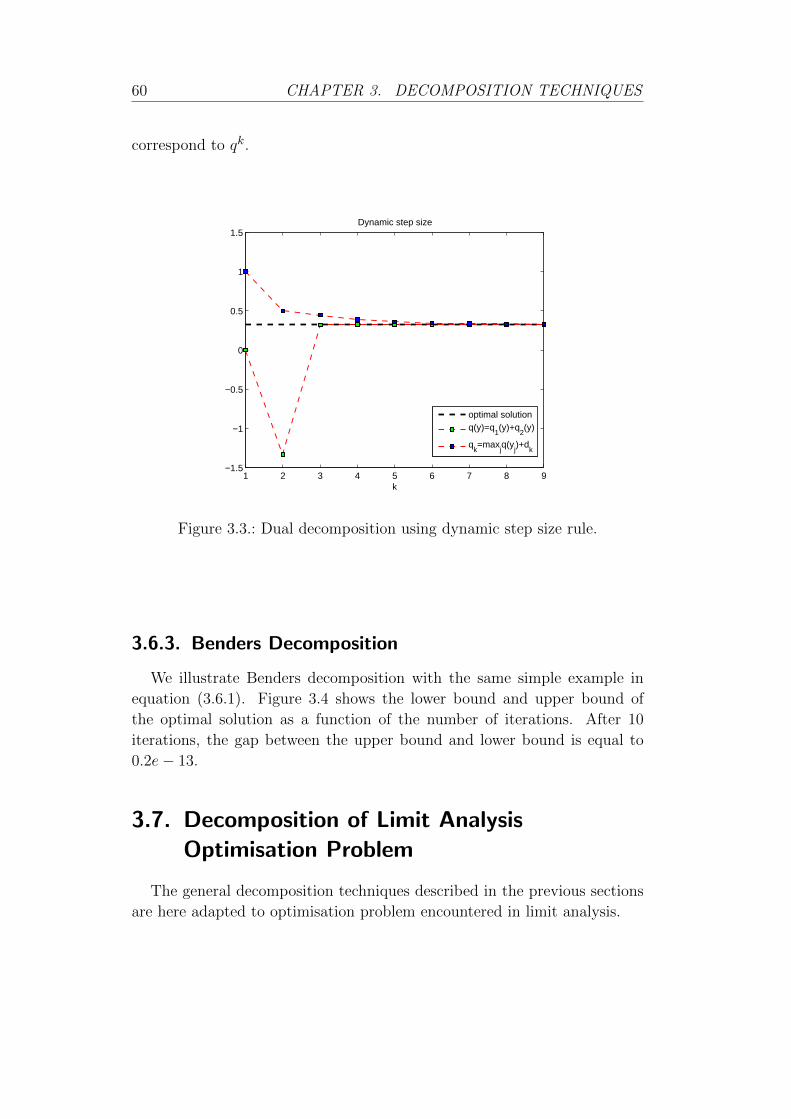
60 CHAPTER 3. DECOMPOSITION TECHNIQUES
correspond to qk.
1 2 3 4 5 6 7 8 9−1.5
−1
−0.5
0
0.5
1
1.5
k
Dynamic step size
optimal solutionq(y)=q
1(y)+q
2(y)
qk=max
jq(y
j)+d
k
Figure 3.3.: Dual decomposition using dynamic step size rule.
3.6.3. Benders Decomposition
We illustrate Benders decomposition with the same simple example in
equation (3.6.1). Figure 3.4 shows the lower bound and upper bound of
the optimal solution as a function of the number of iterations. After 10
iterations, the gap between the upper bound and lower bound is equal to
0.2e− 13.
3.7. Decomposition of Limit Analysis
Optimisation Problem
The general decomposition techniques described in the previous sections
are here adapted to optimisation problem encountered in limit analysis.

CHAPTER 3. DECOMPOSITION TECHNIQUES 61
1 2 3 4 5 6 7 8 9 10−250
−200
−150
−100
−50
0
50
100
Number of iteration
optimal solutionupper boundlower bound
Figure 3.4.: Evolution of upper and lower bound using Benders
decomposition.
3.7.1. Decomposition of LB Problem
As described in Chapter 1, the lower bound (LB) problem of limit analysis
may be stated as the following optimisation problem (see (1.2.5)):
minσ,λ− λ
Aeq1σ + F eq1 = 0
Aeq2σ = 0
Aeq3σ + λF eq3 = 0
σ ∈ B.
(3.7.1)
We translate the ideas of decomposition techniques explained in the previous
sections to (LB) problem of limit analysis.
Decomposition of LB problem corresponds to the split of the stress vari-
ables σ into two sets σ1 and σ2. In view of equation (1.2.6), it means
that the variable x = (x4,x1:3) is split into two variables x1 and x2 where
x1 = (x14,x
11:3) and x2 = (x2
4,x21:3).
As described in Chapter 1 the equation Aeq1σ + λF eq1 = 0 in (1.2.5) is
related to the equilibrium constraint. In view of the structure of matrix Aeq1
in (A.1.4) and how it is built, we can decompose the matrix Aeq1 into two

62 CHAPTER 3. DECOMPOSITION TECHNIQUES
−t
σ1, λ1
t
σ2, λ2
Figure 3.5.: Decomposition of global problem into two subproblems. The
global variables are the boundary traction t at the fictitious
Neumann condition and global load factor λ.
matrixes Aeq1,1 and Aeq1,2. In other words the equality Aeq1σ+λF eq1 = 0
can be split into two equalities as follows:
Aeq1,1σ1 + λF eq1,1 = 0,
Aeq1,2σ2 + λF eq1,2 = 0.(3.7.2)
The split of σ into two vectors σ1 and σ2, it leads to the decomposition
of the domain into two parts, with a common boundary that couples the
common nodes. It means that the vectors σ1 and σ2 are decomposed into
two vectors σ1 = (σ1,1,σ1,2) and σ2 = (σ2,1,σ2,2) such that the vectors
σ1,1 and σ2,2 are coupled. In other words, in view of the structure of matrix
Aeq2 the equation Aeq2σ = 0 in (1.2.5), which is related to the inter-element
equilibrium constraint, can be decomposed into three equations as follows:
Aeq2,1σ1 = 0,
Aeq2,2σ2 = 0,
Beq2,1σ1 + Beq2,2σ2 = 0.
(3.7.3)
We note that the last equation in (3.7.3) is a complicating constraint.
The equation A3σ + λF eq3 = 0, in view of the structure of matrix Aeq3 in

CHAPTER 3. DECOMPOSITION TECHNIQUES 63
equation (A.3.1) can be decomposed as,
Aeq3,1σ1 + λF eq3,1 = 0,
Aeq3,2σ2 + λF eq3,2 = 0.(3.7.4)
Consequently, we can rewrite the optimisation problem in (1.2.5) as,
minxi,λ− λ
(Aeq1,iP)xi4 + (Aeq1,iQ)xi1:3 + λF eq1,i = 0
(Aeq2,iP)xi4 + (Aeq2,iQ)xi1:3 = 0
(Aeq3,iP)xi4 + (Aeq3,iQ)xi1:3 + λF eq3,i = 0
Rixi1:3 = bi
(Beq2,1P)x14 + (Beq2,1Q)x1
1:3 + (Beq2,2P)x24 + (Beq2,2Q)x2
1:3 = 0
xi1:3 ∈ Ki,
xi4, λ are free, (i = 1, 2).(3.7.5)
The last equation in the previous optimisation problem (3.7.5) is a com-
plicating constraint. The variables x1 and x2 can be regarded as local
variables, while the variable λ can be regarded as a global variable. In order
to decompose the problem in (3.7.5) we first introduce a variable t such that
(Beq2,1P)x14 + (Beq2,1Q)x1
1:3 = t,
Then, we can rewrite the optimisation problem in the following form:
mint,xi,λ
− λ
(Aeq1,iP)xi4 + (Aeq1,iQ)xi1:3 + λF eq1,i = 0
(Aeq2,iP)xi4 + (Aeq2,iQ)xi1:3 = 0
(Aeq3,iP)xi4 + (Aeq3,iQ)xi1:3 + λF eq3,i = 0
Rixi1:3 = bi
(Beq2,iP)xi4 + (Beq2,iQ)xi1:3 = (−1)i+1t
xi1:3 ∈ Ki
xi4, t, λ are free, (i = 1, 2).
(3.7.6)
Note that since the complicating constraint in optimisation problem (3.7.5)
is built through the common boundary, the coupling constraint can be in-
terpreted as a fictitious Neumann condition for each subdomain.

64 CHAPTER 3. DECOMPOSITION TECHNIQUES
Let y = (t, λ), xi = (xi4, xi1:3) and Ci, (i = 1, 2) be local constraints that
are defined as follows:
Ci =
[xi
y
]:
(Aeq1,iP)xi4 + (Aeq1,iQ)xi1:3 + λF eq1,i = 0
(Aeq2,iP)xi4 + (Aeq2,iQ)xi1:3 = 0
(Aeq3,iP)xi4 + (Aeq3,iQ)xi1:3 + λF eq3,i = 0
Rixi1:3 = bi
(Beq2,iP)xi4 + (Beq2,iQ)xi1:3 = (−1)i+1t
xi1:3 ∈ Ki, xi4; t, λ are free.
(3.7.7)
Then, problem (3.7.6) reads:
minx1,x2,y
f1(x1,y) + f2(x2,y)
(x1,y) ∈ C1, (x2,y) ∈ C2,
(3.7.8)
where fi(xi,y) = −λ2 .
In the above problem, The variable y is a public or so to speak a com-
plicating variable and the variable xi is called a private variable or local
variable.
We now apply primal and dual decomposition for the optimisation prob-
lem in (3.7.8).
3.7.2. Primal Decomposition (LB)
In primal decomposition, at each iteration we fix the public variable y.
Thus by fixing the variable y, the optimisation problem (3.7.8) is separable.
Each subproblem can separately find optimal values for its local variables
xi. Let us denote, qi(y) the optimal value of the following subproblem:
qi(y) = minxifi(x
i,y)
(xi,y) ∈ Ci,(3.7.9)
with variable xi, as a function of y. The original problem (3.7.8) is equiva-
lent to the primal master problem
minyq(y) = q1(y) + q2(y), (3.7.10)
with variable y. In order to find a subgradient of q, we find gi ∈ ∂qi(y)(which
can be done separately), then we have
g = g1 + g2.

CHAPTER 3. DECOMPOSITION TECHNIQUES 65
3.7.3. Dual Decomposition (LB)
By introducing the new variables ti, λi, yi = (ti, λi), i = 1, 2, and z =
(t, λ) we can rewrite the optmisation problem at (3.7.8) in the following
form:min
x1,x2,y1,y2,zf1(x1,y1) + f2(x2,y2)
y1 − z = 0
y2 − z = 0
(x1,y1) ∈ C1, (x2,y2) ∈ C2.
(3.7.11)
We form the partial Lagrangian of problem (3.7.11),
L(x1,x2,y1,y2, z;v1,v2) =f1(x1,y1) + f2(x2,y2) + v1 · (−y1 + z)+
v2 · (−y2 + z) = (f1(x1,y1)− v1 · y1)+
(f2(x2,y2)− v2 · y2) + (v1 + v2) · z,
where vi is the Lagrangian multiplier associated with yi − z = 0. To find
the dual function, we first minimize over z, which results in the condition
v1 + v2 = 0. In other words,
q(v1,v2) = minx1,x2,y1,y2
(x1,y1)∈C1
(x2,y2)∈C2
minz
(f1(x1,y1)− v1 · y1) + (f2(x2,y2)− v2 · y2) + (v1 + v2) · z,
then
q(v1,v2) = minx1,y1,x2,y2
(x1,y1)∈C1
(x2,y2)∈C2
v1+v2=0
(f1(x1,y1)− v1 · y1) + (f2(x2,y2)− v2 · y2).
We define qi(vi), (i = 1, 2) as the optimal value of the subproblem
qi(vi) = min
xi,yi(fi(x
i,yi)− vi · yi)
(xi,yi) ∈ Ci,(3.7.12)
as a function of vi. A subgradient of qi at vi is just −yi, an optimal value
of yi in the subproblem (3.7.12).
66 CHAPTER 3. DECOMPOSITION TECHNIQUES
Therefore the dual of the original problem (3.7.11) is
max q(v1,v2) = q1(v1) + q2(v2)
ET
v1
v2
= 0,
with variable v1, v2 and ET = [I I]. We can solve this dual decomposition
master problem using a projected subgradient method. The projection onto
the feasible set
(v1,v2)|v1 + v2 = 0
, is using expression in (3.2.2) given
by:
P = I− E(ETE)−1ET .
It can be verified that
P
v1
v2
=
1
2
v1 − v2
v2 − v1
.
3.7.4. Benders Decomposition(LB)
As it can be verified, the lower bound (LB) problem of limit analysis
could be stated as the following structure:
min− λA1x1 + λF 1 = b1
A2x2 + λF 2 = b2
B1x1 + B2x2 = 0
x1 ∈ K1,x2 ∈ K2, λ is free,
(3.7.13)
where K1 and K2 are closed convex cones.
As before, we shall use a free complicating variable t to rewrite the pre-
vious equations as the following two sets of coupled equations,
minx1,x2,λ
− λ
A1x1 + λF 1 = b1
B1x1 + t = 0
x1 ∈ K1
A2x2 + λF 2 = b2
B2x2 − t = 0
x2 ∈ K2.
(3.7.14)

CHAPTER 3. DECOMPOSITION TECHNIQUES 67
The LB optimisation problem can be then restated as the two subprob-
lems,
(Pi) minxi
0 (Di) max(bi − λkF i) · yiλ + (−1)itk · yityiλ : Aixi = bi − λkF i −(AT
i yiλ + BTi yit) ∈ K∗i
yit : Bixi = (−1)itk
xi ∈ Ki.
(i = 1, 2)
(3.7.15)
where tk and λk are the solution of the following master problem:
mint,λ,α1,α2
− λ+ α1 + α2
α1 ≥ (b1 − λF 1) · yk1λ − t · yk1tα2 ≥ (b2 − λF 2) · yk2λ + t · yk2t
, k = 1, 2, . . .(3.7.16)
The inequality constraints in the previous optimisation problem are ap-
plied for all the available optimal dual variables yit and yiλ of the sub-
problems obtained by using different values of tk and λk, k = 1, 2, . . . in
subproblem (3.7.15). The initial values t0 = 0 and λ0 = 0 may be em-
ployed.
The inequality constraint αi ≥ (bi − λF i) · ykiλ + (−1)it · ykit in (3.7.16)
which is obtained by optimal dual variables yit and yiλ of subproblem
(3.7.15) is so called optimality cut. The optimality cut is obtained when
the primal subproblem (Pi) (3.7.15) is feasible and finite. If primal subprob-
lem (Pi) for (λk, tk) is not feasible then in term of the Frakas Lemma B.5,
the dual subproblem (Di) (3.7.15) is infinite, it means that, there exists ykitand ykiλ such that
−(ATi y
kiλ + BT
i ykit) ∈ K∗i and (bi − λkF i) · ykiλ + (−1)itk · ykit > 0.
(3.7.17)
Since K∗i is a cone then we have
β(bi − λkF i) · ykiλ + β(−1)itk · ykit > 0, ∀β > 0,
− β(ATi y
kiλ + BT
i ykit) ∈ K∗i .

68 CHAPTER 3. DECOMPOSITION TECHNIQUES
Thus, when β tends to +∞, the objective function of dual subproblem
(Di) (3.7.15) tends to +∞. In other words, dual subproblem (Di) (3.7.15)
is finite if and only if
(bi − λkF i) · yiλ + (−1)itk · yit ≤ 0, when − (ATi yiλ + BT
i yit) ∈ K∗i .
Consequently we append these constraints which are so called feasibility
cuts to the master problem to ensure that the dual is always bounded.
By modifying the primal subproblem (Pi) in (3.7.15) as follows, we obtain
either feasibility cut or optimality cut :
(Pi) : min s+i + s−i + e ·w+
i + e ·w−iyiλ : Aixi + s+
i F i − s−i F i = bi − λkF i
yit : BTi xi + Iw+
i − Iw−i = (−1)itk
xi ∈ Ki, s+i ≥ 0, s−i ≥ 0,w+
i ≥ 0,w−i ≥ 0
(3.7.18)
(Di) : max(bi − λkF i) · yiλ + (−1)itk · yit− (AT
i yiλ + BTi yit) ∈ K∗i
− 1 ≤ F iyiλ ≤ 1
− e ≤ yit ≤ e
(3.7.19)
where e is a vector that all components are equal 1.
If the optimal solution of primal problem (Pi) (3.7.18) is zero, then we
have optimality cut, and if it is strictly positive, we have feasibility cuts.
The full master problem with feasibility and optimality cuts is obtained as
follows :
mint,λ,α1,α2
− λ+ α1 + α2
α1 ≥ (b1 − λF 1) · yk1λ − t · yk1tα2 ≥ (b2 − λF 2) · yk2λ + t · yk2t
, k = 1, 2, . . .
0 ≥ (b1 − λF 1) · yl1λ − t · yl1t0 ≥ (b2 − λF 2) · yl2λ + t · yl2t
, l = 1, 2, . . .
(3.7.20)
Now we apply the Benders decomposition method for the following differ-
ent sizes of LB problem with the same structure defined in (3.7.13). The size
of the problems are given in Table 3.1, where n and m denote the number
of rows and and columns of matrix A in (1.2.5), and nT is the total number

CHAPTER 3. DECOMPOSITION TECHNIQUES 69
Problem n m nTa 96 97 20
b 368 385 101
c 2240 2401 700
Table 3.1.: Size and total master iterations of each problem solved using
SDPT3 [47].
of master iterations. The problems have been solved using the optimisation
software SDPT3 [47]. Figure 3.6 shows exact global optimal solution and
optimal solution of master problem at each iteration respectively.
As it can be observed, the number of iteration increases dramatically due
to nonlinearity of the conic constraints, which can not be properly repre-
sented with the linear feasibility and optimality cuts. This fact motivates,
the use of the proposed method in the next Chapter.

70 CHAPTER 3. DECOMPOSITION TECHNIQUES
0 5 10 15 20−4.5
−4
−3.5
−3
−2.5
−2
−1.5
Number of master iterations
Optimal valueSolutions of master problem
(a)
0 20 40 60 80 100 120−4.5
−4
−3.5
−3
−2.5
−2
Number of master iterations
solutions of master problemOptimal value
(b)
0 200 400 600 800−5
−4
−3
−2
−1
0
Number of master iterations
Optimal valueSolutions of master problem
(c)
Figure 3.6.: Benders decomposition, apply to the LB limit analysis problem.

4AAR-Based Decomposition Algorithm for
Non-linear Convex Optimisation
4.1. Alternative Definition of Global Feasibility
Region
The objective of this section is to provide a description of a decomposition
method that exploits the results of the AAR method given in Chapter 2. The
method is suitable for convex optimisation problems that have the structure
given in (1.2.7), which we aim to transform into the computation of the
minimal distance between two feasible sets. For this aim, we rewrite problem
(1.2.7) by introducing a new complicating variable t as follows:
λ∗ = maxx1,x2,λ,t
λ
f1(x1, λ) = 0
f2(x2, λ) = 0
g1(x1) = t
g2(x2) = −tx1 ∈ K1, x2 ∈ K2, λ ∈ <.
(4.1.1)
We next define the feasibility region of this problem with the help of the
following definitions:
Definition 4.1 Consider the following two feasibility regions:
X1(λ) = x1|f1(x1, λ) = 0 ∩K1,
X2(λ) = x2|f2(x2, λ) = 0 ∩K2,(4.1.2)
71

72 CHAPTER 4. AAR-BASED DECOMPOSITION ALGORITHM
and also let λ = λ be a given real value. Then, we define the following
feasibility sets for variable t:
Z(λ) = g1(X1(λ)) = g1(x1)|x1 ∈ X1(λ),W (λ) = −g2(X1(λ)) = −g2(x2)|x2 ∈ X2(λ).
(4.1.3)
Throughout the subsequent sections, the sets Z(λ) and W (λ) defined in
(4.1.3) are assumed closed and convex. In addition, the functions f1,f2, g1
and g2 are affine maps.
By using definitions (4.1.2) and (4.1.3), the optimisation problem in
(4.1.1) may be recast as,
λ∗ = maxλλ
Z(λ) ∩W (λ) 6= ∅.(4.1.4)
The algorithm proposed in this Chapter is based on the form (4.1.4). In
brief, the algorithm consists on updating the value of λ (master problem)
and analysing in the subproblems whether the intersection between the sets
Z(λ) and W (λ) is empty or not, or equivalently, whether d(W (λ), Z(λ)) > 0.
According to the definitions in Section 2.2 we have that:
d(W (λ), Z(λ)) = infx1∈X1(λ)x2∈X2(λ)
||g1(x1) + g2(x2)|| (4.1.5)
where Xi(λ), i = 1, 2 is defined in (4.1.2).
In order to determine this and compute upper bounds of the global prob-
lem in (4.1.1), we will need the following two propositions:
Proposition 4.1 Let λ0 and λ be given real values such that (x01,x02, t0, λ0)
is a feasible solution for problem (4.1.1), and λ0 < λ. After using the defi-
nition in (4.1.3), the following relation holds:
Z(λ) ∩W (λ) 6= ∅ ⇐⇒ λ ≤ λ∗.
Proof 7 First suppose that Z(λ)∩W (λ) 6= ∅ and t belongs to Z(λ)∩W (λ),
thus there exist x1 ∈ X1(λ) and x2 ∈ X2(λ) such that g1(x1) = t and
−g2(x2) = t. Therefore, in view of (4.1.2), (x1,x2, λ, t) is a feasible solu-
tion for problem (4.1.1), and consequently λ ≤ λ∗.
Conversely, let λ0 < λ < λ∗. Hence, there exists γ ∈ (0, 1) such that
λ = (1− γ)λ0 + γλ∗. Since (x01,x02, t0, λ0) and (x∗1,x∗2, t∗, λ∗) are feasible

CHAPTER 4. AAR-BASED DECOMPOSITION ALGORITHM 73
solutions for problem (4.1.1) and since the feasible region of problem (4.1.1)
is convex, it follows that the convex combination of these two points is a
feasible solution for problem (4.1.1). Formally, we have that
(1− γ)(x01,x02, t0, λ0) + γ(x∗1,x∗2, t∗, λ∗)
= ((1− γ)x01 + γx∗1, (1− γ)x02 + γx∗2, (1− γ)t0 + γt∗, (1− γ)λ0 + γλ∗))
= ((1− γ)x01 + γx∗1, (1− γ)x02 + γx∗2, (1− γ)t0 + γt∗, λ),
which shows that (1− γ)t0 + γt∗ belongs to Z(λ) ∩W (λ), i.e.
Z(λ) ∩W (λ) 6= ∅.
Proposition 4.2 Let (t, λ) be an arbitrary given vector and ∆si, i = 1, 2,
be optimal solutions of the following optimisation problems:
∆si = maxxi,∆w,∆si
∆si
f i(xi, λ+ ∆si) = 0
gi(xi) = (−1)i+1(t+ ∆wi)
xi ∈ Ki, ∆wi ∈ <nm , ∆si ∈ <,
(4.1.6)
with i=1,2. Then λ∗ ≤ λ+ ∆si.
Proof 8 There exists a real value ∆s∗ and a vector ∆w∗ such that
λ∗ = λ+ ∆s∗;
t∗ = t+ ∆w∗.(4.1.7)
Since (x∗1,x∗2, t∗, λ∗) is a feasible solution for problem (4.1.1), and in view
of (4.1.7) we have that
f i(x∗i , λ∗) = 0
gi(x∗i ) = (−1)i+1t∗
x∗i ∈ Ki
⇒
f i(x∗i , λ+ ∆s∗) = 0
gi(x∗i ) = (−1)i+1(t+ ∆w∗)
x∗i ∈ Ki, ∆w∗ ∈ <nm , ∆s∗ ∈ <.
But since ∆si is an optimal solution of problem (4.1.6), it follows from
(4.1.7) that
∆s∗ ≤ ∆si ⇒ λ+ ∆s∗ ≤ λ+ ∆si ⇒ λ∗ ≤ λ+ ∆si.
74 CHAPTER 4. AAR-BASED DECOMPOSITION ALGORITHM
It will become convenient to consider the dual form of the global problem
(1.2.7),
q∗ = infy1,y2,y3
q(y1,y2,y3) (4.1.8)
where
q(y1,y2,y3) = supx1,x2,λ
y1 · f1(x1, λ) + y2 · f2(x2, λ)
+ y3 · (g1(x1) + g2(x2)) + λ
x1 ∈ K1, x2 ∈ K2, λ ∈ <.
(4.1.9)
4.2. Definition of Subproblems
Let λ0 and λ be given real values such that (x01,x02, λ0) is a feasible
solution for (1.2.7) and λ0 < λ, which means that W (λ) and Z(λ) are
nonempty (closed convex) sets. Take t0 and set
tn = Tn(t0) = T (tn−1), n = 1, 2, 3, · · · ,
where
T =RWRZ + I
2= PWRZ − PZ + I, (4.2.1)
is the transformation of the AAR method described in Section 2.2.
We next define the optimisation subproblems that will allow us to retrieve
the projections PZ and PW , required for computing the transformation T . In
view of (2.2.1), PZ(tn) can be obtained by solving the following optimisation
problem:
minz‖z − tn‖
z ∈ Z(λ),
which is equivalent to the following so-called Subproblem 1 :
minx1,d
1‖d1‖
f1(x1, λ) = 0
g1(x1)− d1 = tn
x1 ∈ K1.
(4.2.2)

CHAPTER 4. AAR-BASED DECOMPOSITION ALGORITHM 75
From the optimal solution of Subproblem 1, d1n, we can compute the
projection PZ(tn) and reflection RZ(tn) as,
PZ(tn) = g1(x1n) = tn + d1n, with x1n ∈ X1(λ),
RZ(tn) = 2PZ(tn)− tn = tn + 2d1n.
(4.2.3)
From PZ(tn), the point PWRZ(tn) = PW (tn+2d1n) is obtained by solving
the following optimisation problem:
minw‖w −RZ(tn)‖
w ∈ W (λ),
which is equivalent to the following so-called Subproblem 2:
minx2,d
2‖d2‖
f2(x2, λ) = 0
g2(x2) + d2 = −RZ(tn)
x2 ∈ K2,
(4.2.4)
with RZ(tn) = tn + d1n, (see 4.2.3).
After solving this problem we have that,
PWRZ(tn) = −g2(x2n) = RZ(tn) + d2n = tn + 2d1
n + d2n, with x2n ∈ X2(λ)
RWRZ(tn) = 2PW (RZ(tn))−RZ(tn) = tn + 2d1n + 2d2
n,(4.2.5)
and according to (4.2.1),(4.2.3) and (4.2.5),
tn+1 = T (tn) = tn + d1n + d2
n, (4.2.6)
with d1n and d2
n optimal solutions of (4.2.2) and (4.2.4), respectively. This
iterative process and the associated projections and reflections are illustrated
in Figure 4.1. Since T is nonexpansive, and in view of (4.2.1), (4.2.3),(4.2.5)
and (4.2.6), we have the following results,
(i) tn+1 − tn = d1n + d2
n = T (tn)− tn =
PW (RZ(tn))− PZ(tn) = −g2(x2n)− g1(x1n). (4.2.7)
(ii) ‖d1n + d2
n‖ = ‖tn+1 − tn‖ = ‖T (tn)− T (tn−1)‖ ≤‖tn − tn−1‖ = ‖d1
n−1 + d2n−1‖. (4.2.8)

76 CHAPTER 4. AAR-BASED DECOMPOSITION ALGORITHM
Figure 4.1.: Illustration of the iterative process
According to (4.2.8), the sequence (‖d1n + d2
n‖)n∈N is decreasing. There-
fore, we can define the following parameter:
α = infn≥1‖d1
n + d2n‖ = lim
n→∞‖d1
n + d2n‖ ∈ [0,∞), (4.2.9)
which measures the distance d(W (λ), Z(λ)). The next theorem relates α to
the optimal objective λ∗:
Theorem 4.1 Consider Subproblem 1 and Subproblem 2 defined in (4.2.2)
and (4.2.4) respectively. Let λ0 < λ, with (x01,x0,2, λ0) a feasible solution
of the global problem in (1.2.7) and λ∗ its optimal solution. Then, with α
defined in (4.2.9), and if λ∗ = q∗, i.e. there is no duality gap in (4.1.8), the
following implications hold:
(i) α = 0 if and only if λ ≤ λ∗.
(ii) α > 0 if and only if λ > λ∗.
Proof 9 (i): If α = 0, we have from (4.2.7) that
limn→∞
‖d1n + d2
n‖ = limn→∞
‖g1(x1n) + g2(x2n)‖ = 0. (4.2.10)
CHAPTER 4. AAR-BASED DECOMPOSITION ALGORITHM 77
Since (x1n,x2n) ∈ X1(λ) × X2(λ), the vector (x1n,x2n, λ) satisfies the
following conditions:f1(x1n, λ) = 0
f2(x2n, λ) = 0
x1n ∈ K1, x2n ∈ K2.
(4.2.11)
Suppose that (y1,y2,y3) is an arbitrary feasible solution for the dual prob-
lem in (4.1.8). Since (x1n,x2n, λ) ∈ X1(λ)×X2(λ)×<, according to (4.1.9)
we have that
q(y1,y2,y3) ≥y1 · f1(x1n, λ) + y2 · f2(x2n, λ)+
y3 · (g1(x1n) + g2(x2n)) + λ =
y3 · (g1(x1n) + g2(x2n)) + λ,
and then
q(y1,y2,y3) ≥ limn→∞
y3 · (g1(x1n) + g2(x2n)) + λ.
Therefore, in view of (4.2.10), we have that q(y1,y2,y3) ≥ λ. On the
other hand, since (y1,y2,y3) is an arbitrary feasible solution for the dual
problem, and due to assumption q∗ = λ∗, we have the following result :
λ ≤ infy1,y2,y3
q(y1,y2,y3) = q∗ = λ∗ ⇒ λ ≤ λ∗.
Conversely, assume λ ≤ λ∗. Thus, in view of Lemma 2.6 and Propo-
sitions 2.5 and 4.1, we can infer that the sequence (tn)n∈N converges to a
point in Fix T , i.e.
limn→∞
tn = t ∈ Fix T.
Since tn+1 − tn = d1n + d2
n, we deduce that,
limn→∞
d1n + d2
n = limn→∞
tn+1 − tn = t− t = 0⇒ α = limn→∞
‖d1n + d2
n‖ = 0.
(ii) Since α ≥ 0, the result in (ii) follows from (i).
The result of Theorem 4.1 is illustrated in Figure 4.2, which represents
the distance of the sets Z(λ) and W (λ) for the cases λ ≤ λ∗ and λ > λ∗.
Figure 4.3 also shows the same idea but on the (λ, t) plane. Consequently,
the optimisation problem in (4.1.4) also reads:
λ∗ = maxλλ
d(W (λ), Z(λ)) = 0(4.2.12)

78 CHAPTER 4. AAR-BASED DECOMPOSITION ALGORITHM
Note that for a given value of λ, from the result in Theorem 4.1(ii),
Proposition 4.1, and Lemma 2.6, we infer the following corollary :
Corollary 1 α > 0 ⇐⇒ ‖tn‖ → ∞.
According to this corollary and Lemma 2.6 (iv), the values of ‖ tnn ‖ and
‖tn‖ could be used to monitor the gap between Z(λ) and W (λ). We will
though use other parameters to monitor this distance, as explained in the
next section.
Figure 4.2.: Illustration of the sets W (λ) and Z(λ) for the case λ ≤ λ∗ and
λ > λ∗.
4.3. Algorithmic Implementation of AAR-based
Decomposition Algorithm
As it has been explained in the previous sections, the objective is to solve
an optimisation problem with the structure in (1.2.7), recasted in the form
in (4.1.1).
The master problem computes at each master iteration k a new value of
λk, while the subproblems determine whether this value λk is an upper or

CHAPTER 4. AAR-BASED DECOMPOSITION ALGORITHM 79
Figure 4.3.: Illustration of the sets W (λ) and Z(λ) on the (λ, t) plane.
lower bound of λ∗. To determine this, a set of nk subiterations, n = 1, . . . , nkare required at each master iteration k.
The procedure of the master and subproblems are detailed in next two
subsections, which use the following notation:
• αn = ‖d1n + d2
n‖, βn = ‖d1n‖+ ‖d2
n‖.
• ∆αn = αn − αn−1.
Also λklb, λkub denote algorithmic lower and upper bounds of λ∗ in the
master iteration k, respectively.
4.3.1. Master Problem
The steps that define the master problem are given in Box 1.
M0. Find real values λ0lb and λ0
ub such that λ∗ ∈ [λ0lb, λ
0ub]. Set k = 1.
M1. Set λk = (1− s)λk−1lb + sλk−1
ub , s ∈ (0, 1) (k = 1, 2, · · · ).
M3. Solve Subproblems in Box 2 to determine whether λk ≤ λ∗ or
λ∗ < λk.

80 CHAPTER 4. AAR-BASED DECOMPOSITION ALGORITHM
M4. If |λkub − λklb| ≤ ελ
• λ∗ ≈ λk,
• Stop.
Else
• k = k + 1,
• Go to M1,
End.
Box 1. Master problem
In step M1, λ0lb is a feasible solution for problem (4.1.1), which means that
it exists a vector t such that t ∈ Z(λ0lb) ∩W (λ0
lb), with W (λ0lb) and Z(λ0
lb)
defined in (4.1.3). λ0ub is an arbitrary upper bound for λ∗ that can be ob-
tained via any possible way. In this article, we use Proposition 4.2 to obtain
an upper bound of λ∗: we solve two subproblems defined in (4.1.6), and we
obtain two upper bounds λ01ub and λ0
2ub. Then we set λ0ub = min(λ0
1ub, λ02ub).
In step M1, if X1(λk−1ub ) 6= ∅ and X2(λk−1
ub ) 6= ∅ defined in (4.1.2), we
clearly have that X1(λk) 6= ∅ and X2(λk) 6= ∅, since f1,f2, g1, g2 are affine
functions and K1, K2 are convex sets. The constant value s = 12 has been
employed for the update of λk in Box 1, Step M1.
4.3.2. Subproblems
The iterative process of each subproblem is summarised in Box 2.
S1. Set λ = λk, tk0 = tk−1, n = 0.
S2. Solve Subproblem 1 defined in (4.2.2). Obtain d1n and set tkn =
tkn + 2d1n.
S3. Solve Subproblem 2 defined in (4.2.4). Obtain d2n and set tkn =
tkn + 2d2n.
S4. Set βn = ‖d1n‖+ ‖d2
n‖ and αn = ‖d1n + d2
n‖.

CHAPTER 4. AAR-BASED DECOMPOSITION ALGORITHM 81
S5. If βn < βn−1 or αn ≤ ε0, then λk ≤ λ∗:
• λklb = λk, λkub = λk−1ub . Update ∆k.
• Go to Box 1.M1.
Else if βn > βn−1 and αn >∆k−1
k and|∆αn||αn| < ε1, then λk > λ∗:
• λklb = λk−1lb , λkub = λk. Update ∆k.
• Go to Box 1.M1.
Else
• tkn =tkn−1+tkn
2 , n = n+ 1,
• Go to S2.
End
Box 2. Subproblems 1 and 2.
The algorithm in Box 2 uses the control parameters βn, αn and ∆k to
detect whether λk is an upper bound or a lower bound of λ∗ . Indeed, the
numerical results show that βn decreases when λk is a lower bound of λ∗.
The values of βn satisfy in fact the following corollary:
Corollary 2 Assume that λ is a given real value and W = W (λ), Z = Z(λ)
defined in (4.1.3). Then the following relations hold.
(i) : If 0 ∈ int(W ∩ Z) then limn→∞ βn = 0.
(ii) : If limn→∞ βn = 0 then W ∩ Z 6= ∅.
Proof 10 (i) : Since 0 ∈ int(W ∩ Z), then W ∩ Z 6= ∅, and it follows that
Fix PW 6= ∅,Fix PZ 6= ∅, and also Fix PWPZ = Fix PW ∩Fix PZ . According
to the AAR method, since W ∩ Z 6= ∅, we have that
limn→∞
tn = t ∈ Fix T.
On the other hand, since 0 ∈ int(W ∩ Z), then Fix T = W ∩ Z [7], and
therefore we have in turn that,
PZ(t) = t, PW (t) = t, RZ(t) = 2PZ(t)− t = t. (4.3.1)

82 CHAPTER 4. AAR-BASED DECOMPOSITION ALGORITHM
In view of (4.2.3), (4.2.6) and (4.3.1) , the following results can be de-
rived:limn→∞
d1n = lim
n→∞PZ(tn)− tn = PZ(t)− t = 0
limn→∞
d2n = lim
n→∞tn+1 − tn − d1
n = 0.(4.3.2)
Consequently, in view of (4.3.2), we infer that
limn→∞
βn = limn→∞
‖d1n‖+ ‖d2
n‖ = 0. (4.3.3)
(ii) : For each iteration n we have that αn = ‖d1n+d2
n‖ ≤ ‖d1n‖+‖d2
n‖ = βn.
Therefore,
0 = limn→∞
βn ≥ limn→∞
αn = α ≥ 0, (4.3.4)
which implies that α = 0. Consequently, in view of Proposition 4.1 and
Theorem 4.1, we infer that W ∩ Z 6= ∅.
We note that the update of λk in step M1 of the master problem mimics
the update process of the bisection method. Other faster updates could be
envisaged, but at the expense of estimating more accurately the distance be-
tween the sets W (λk) and Z(λk). In our implementation of the subproblems,
we just detect from the trends of βn and αn whether the set W (λk)∩Z(λk)
is empty or not, but do not actually compute the distance d(W (λk), Z(λk)).
The accurate computation of the distance would require far more subiter-
ations, and in the authors experience, this extra cost does not compensate
the gain when more sophisticated updates for λk are implemented.
The algorithms in Box 1 and 2 use three tolerance parameters: ελ, ε0 and
ε1. Their meaning is the following:
• ελ: this is the desired tolerance for the objective λ, and it is such that
λ∗ ∈ [λlb, λub], with |λub − λlb| < ελ.
• ε0: is a tolerance for d(W (λk), Z(λk)). If d(W (λk), Z(λk)) < ε0, we
will consider that W (λk) ∩ Z(λk) 6= ∅.
• ε1 is used to detect when the sequence αn (generated by the solution
of subproblems) has converged

CHAPTER 4. AAR-BASED DECOMPOSITION ALGORITHM 83
In all our numerical tests, we have used the values (ελ, ε0, ε1) = (10−3, 5∗10−4, 10−2). The vectors (tk,xk1,x
k2) resulting from the subproblems for
the highest (latest) value of λklb furnish the algorithmic approximations of
(t∗,x∗1,x∗2). In addition, the algorithm in Box 2 uses the parameter ∆k to
control the convergence of αn, which is an approximation to d(W (λk), Z(λk).
We suggest two possible updates:
U1:
• If λk ≤ λ∗, then ∆k = λk−1ub − λk.
• If λk > λ∗, then ∆k = λk − λk−1lb .
U2:
• If λk ≤ λ∗, then ∆k = ∆k−1.
• If λk > λ∗, then ∆k = s||d1n − d2
n||.
Figure 4.4 illustrates the update proposed in U1. The update given in U2,
will be justified in the next section.
(a)
(b)
Figure 4.4.: Updating parameter ∆k. (a): λk is considered as an upper
bound, (b): λk is considered as a lower bound.

84 CHAPTER 4. AAR-BASED DECOMPOSITION ALGORITHM
4.3.3. Justification of Update U2 for ∆k
The aim of the update suggested here is to avoid obtaining false lower
bounds, false upper bounds, or endless loops. Indeed, large values of ∆k, will
prevent the algorithm from stopping when λk is an upper bound (endless
loop), and small values of ∆k may give false upper bounds, i.e. a value
λk < λ∗ that is detected as an upper bound.
Throughout this subsection, λlb and λub denote a feasible lower bound
and an upper bound of problem (4.1.1) respectively. Note that we may have
that λlb = λ∗.
Proposition 4.3 Let us denote by α(λ) the distance between two sets Z(λ)
and W (λ) defined in (4.1.3), as a function of λ i.e.
α(λ) = d(Z(λ),W (λ)) = infx1∈X1(λ)x2∈X2(λ)
||g1(x1) + g2(x2)||, (4.3.5)
where X1(λ) and X2(λ) are defined in (4.1.2). Then the following hold:
(i) If λs = (1− s)λlb + sλub with s ∈ (0, 1), then α(λs) ≤ sα(λub).
(ii) α(λ) is strictly increasing on [λ∗, λub].
(iii) limλ→λ∗ α(λ) = 0 with λ ∈ (λ∗, λub].
(iv) Let s ∈ (0, 1) be a constant parameter that has been used to generate
a sequence (λkub)k∈N of upper bounds of λ∗ in the following manner:
λ0ub = λub
λkub = (1− s)λlb + sλk−1ub , k = 1, 2, · · ·
(4.3.6)
Then α(λkub) ≤ (s)kα(λub).
(v) α(λ) is a convex function on [λ∗, λub].
Proof 11 (i) :Let (x1ub,x2ub) ∈ X1(λub)×X2(λub) and (x1lb,x2lb) ∈ X1(λlb)×X2(λlb) with g1(x1lb) + g2(x2lb) = 0. Set :
(xi, λs) = (1− s)(xilb, λlb) + s(xiub, λub) (i = 1, 2). (4.3.7)
According to the definition of the set Xi(λs), the vector xi obviously be-
longs to Xi(λs), (i = 1, 2).

CHAPTER 4. AAR-BASED DECOMPOSITION ALGORITHM 85
Since the functions g1 and g2 are both affine maps then we have:
g1(x1) + g2(x2) =
g1((1− s)x1lb + sx1ub) + g2((1− s)x2lb + sx2ub) =
(1− s)(g1(x1lb) + g2(x2lb)) + s(g1(x1ub) + g2(x2ub)) =
s(g1(x1ub) + g2(x2ub)).
(4.3.8)
Thus in view of (4.3.8) and (4.3.5) we have that :
α(λs) ≤ ||g1(x1) + g2(x2)|| = s||g1(x1ub) + g2(x2ub)||,
and since xiub is an arbitrary element of Xi(λub),
α(λs) ≤ sα(λub).
(ii) Assume that λ∗ < λ1 < λ2 ≤ λub. Then there exists s ∈ (0, 1)
such that λ1 = (1 − s)λ∗ + sλ2, and according to (i) we have that α(λ1) ≤sα(λ2) < α(λ2), i.e. α(λ) is strictly increasing on [λ∗, λub].
(iii) The results in (iii) and (iv) easily follow from (i).
(v) Fix λ1 and λ2 in (λ∗, λub], and t ∈ (0, 1). Set λ = (1 − t)λ1 + tλ2.
Now let (z1, z2) ∈ X1(λ1)×X2(λ1) and (w1,w2) ∈ X1(λ2)×X2(λ2). Then
according to the definition of the set Xi(λj) :
(1− t)zi + twi ∈ Xi(λ), (i = 1, 2). (4.3.9)
It follows from definition of α(λ) in (4.3.5), that
α(λ) ≤ ||g1((1− t)z1 + tw1) + g2((1− t)z2 + tw2)||. (4.3.10)
Since gi, (i = 1, 2) is an affine map, we have that:
||g1((1− t)z1 + tw1) + g2((1− t)z2 + tw2)|| =||(1− t)(g1(z1) + g2(z2)) + t(g1(w1) + g2(w2))|| ≤(1− t)||g1(z1) + g2(z2)||+ t||g1(w1) + g2(w2)||.
(4.3.11)
Thus, in view of (4.3.10) and (4.3.11),
α(λ) = α((1− t)λ1 + tλ2) ≤ (1− t)α(λ1) + tα(λ2),
i.e. α(λ) is convex.
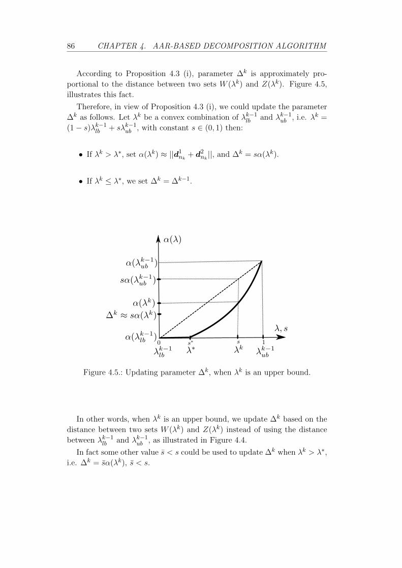
86 CHAPTER 4. AAR-BASED DECOMPOSITION ALGORITHM
According to Proposition 4.3 (i), parameter ∆k is approximately pro-
portional to the distance between two sets W (λk) and Z(λk). Figure 4.5,
illustrates this fact.
Therefore, in view of Proposition 4.3 (i), we could update the parameter
∆k as follows. Let λk be a convex combination of λk−1lb and λk−1
ub , i.e. λk =
(1− s)λk−1lb + sλk−1
ub , with constant s ∈ (0, 1) then:
• If λk > λ∗, set α(λk) ≈ ||d1nk + d2
nk ||, and ∆k = sα(λk).
• If λk ≤ λ∗, we set ∆k = ∆k−1.
Figure 4.5.: Updating parameter ∆k, when λk is an upper bound.
In other words, when λk is an upper bound, we update ∆k based on the
distance between two sets W (λk) and Z(λk) instead of using the distance
between λk−1lb and λk−1
ub , as illustrated in Figure 4.4.
In fact some other value s < s could be used to update ∆k when λk > λ∗,
i.e. ∆k = sα(λk), s < s.

CHAPTER 4. AAR-BASED DECOMPOSITION ALGORITHM 87
4.4. Mechanical Interpretation of AAR-based
Decomposition Method
Consider the following global form of the problem in (1.2.5):
λ∗ = maxσ,λ
λ
∇ · σe,LBi + λf ei = 0 in Ωei ,∀ e = 1, · · · , nei
(σe,LBi − σe′,LBi ) · nξ
e′e
i = 0, ∀ ξe′e ∈ ξOiσe,LBi · nξ
Ne
i = λgξNe ∀ ξNe ∈ ξNi
σe,LBi · nξNe
i = (−1)it ∀ ξNe ∈ ξNiσe,LBi ∈ B in Ωe
i , ∀ e = 1, · · · , nei
(i = 1, 2)
(4.4.1)
where ξNi indicates the fictitious Neumann, at each subdomain that is, the
common domain of the two subdomains (see Figure 4.6). t is in fact the
traction vector t = σ · n along this common boundary. By solving the
following two subproblems, where t is left as a free variable, not necessarily
equal of each subdomain, we obtain upper bounds for λ∗ :
λ∗i = maxσ,λ,t
λ
∇ · σe,LBi + λf ei = 0 in Ωei ,∀ e = 1, · · · , nei
(σe,LBi − σe′,LBi ) · nξ
e′e
i = 0, ∀ ξe′e ∈ ξOiσe,LBi · nξ
Ne
i = λgξNe ∀ ξNe ∈ ξNi
σe,LBi · nξNe
i = (−1)it ∀ ξNe ∈ ξNiσe,LBi ∈ B in Ωe
i , ∀ e = 1, · · · , nei,
(4.4.2)
that is, λ∗ ≤ λ∗i , i = 1, 2. At each master iteration, we choose a value of
the load factor λk, and detect whether, there exists a common value of the
traction t such that the global domain is in equilibrium. In other words,
we detect whether the two subdomain can be in equilibrium for the given
load factor λk. More specifically, we set λ = λ and solve the following two
optimisation problems sequentially, in order to detect if λ ≤ λ∗ or λ∗ < λ.

88 CHAPTER 4. AAR-BASED DECOMPOSITION ALGORITHM
Figure 4.6.: Decomposition of global problem into two subproblems. The
global variables are the boundary traction t at the fictitious
Neumann condition and global load factor λ.
Subproblem 1
‖d1n‖ = min
σ,d1‖d1‖
∇ · σe,LB1 + λf e1 = 0 in Ωe1 ,∀ e = 1, · · · , ne1
(σe,LB1 − σe′,LB
1 ) · nξe′e
1 = 0, ∀ ξe′e ∈ ξO1σe,LB1 · nξ
Ne
1 = λgξNe ∀ ξNe ∈ ξN1
σe,LB1 · nξNe
1 = tn + d1 ∀ ξNe ∈ ξN1σe,LB1 ∈ B in Ωe
1, ∀ e = 1, · · · , ne1.
(4.4.3)
CHAPTER 4. AAR-BASED DECOMPOSITION ALGORITHM 89
Subproblem 2
‖d2n‖ = min
σ,d2‖d2‖
∇ · σe,LB2 + λf e2 = 0 in Ωe2 ,∀ e = 1, · · · , ne2
(σe,LB2 − σe′,LB
2 ) · nξe′e
2 = 0, ∀ ξe′e ∈ ξO2σe,LB2 · nξ
Ne
2 = λgξNe ∀ ξNe ∈ ξN2
σe,LB2 · nξNe
2 = −tn − 2d1n − d2 ∀ ξNe ∈ ξN2
σe,LB2 ∈ B in Ωe2, ∀ e = 1, · · · , ne2.
(4.4.4)
Update t :
tn+1 = tn + d1n + d2
n.
If tn+1 = tn i.e. ||d1n−d2
n|| = 0, then a common traction field t = tn that
equilibrates the two subdomains has been found and λk ≤ λ∗. Otherwise, if
for all n, ||d1n + d2
n|| > 0, no common value of t can be found for the chosen
load factor λk and therefore λ∗ < λk.
Note: The algorithm that computes the approximate value of λ∗ has
been implemented both in MATLAB and FORTRAN90.
In the next section the AAR-based decomposition method is illustrated
and is applied for problems in limit analysis.
4.5. Numerical Results
4.5.1. Illustrative Example
We illustrate the AAR-based decomposition technique explained in pre-
vious section with a toy nonlinear convex problem given by,
λ∗ = maxλ,x1,x2
λ
A1x1 + λF 1 = b1
A2x2 + λF 2 = b2
G1x1 + G2x2 = b
x1 ∈ K1, x2 ∈ K2, λ ∈ <,
(4.5.1)
where K1 and K2 are second-order cones and x1 ∈ <4, x2 ∈ <4. The values
of matrix Ai,Gi and vectors F i, bi and b are given next, and the optimal

90 CHAPTER 4. AAR-BASED DECOMPOSITION ALGORITHM
value of this problem is λ∗ = 1.1965.
maxλ,x1,x2
λ
A1︷ ︸︸ ︷[1 −1 0 0
1 0 0 1
]x1 + λ
F 1︷︸︸︷1
1
=
b1︷ ︸︸ ︷1.2
2.4
A2︷ ︸︸ ︷[−1 1 0 0
1 0 0 1
]x2 + λ
F 2︷︸︸︷1
1
=
b2︷ ︸︸ ︷3.2
0.2
G1︷ ︸︸ ︷[0 2 1 0
0 2 0 1
]x1 +
G2︷ ︸︸ ︷[0 2 1 1
0 2 0 1
]x2 =
b︷ ︸︸ ︷1.2
6.2
=
b3︷ ︸︸ ︷−0.8
3.2
+
b4︷︸︸︷2
3
x1 ∈ K1,x2 ∈ K2, λ ∈ <
By selecting arbitrary vectors b3 and b4 such that b = b3 + b4 and
introducing a new variable t, the problem (4.5.1) is written in the following
form,max
λ,x1,x2,λ,tλ
A1x1 + λF 1 = b1
G1x1 − b3 = t
A2x2 + λF 2 = b2
G2x2 − b4 = −tx1 ∈ K1, x2 ∈ K2, λ ∈ <, t ∈ <m.
(4.5.2)
In view of (4.5.2), for any given λ = λ, we have the two feasible sets
defined in (4.1.3), which now take the following form :
Z(λ) = t |G1x1 − b3 = t, A1x1 + λF 1 = b1 for some x1 ∈ K1,W (λ) = t |G2x2 − b4 = −t, A2x2 + λF 2 = b2 for some x2 ∈ K2.
For solving this problem we first take (λ0lb, t) = (0,0) and, according to
Proposition 4.2, after solving the two optimisation problem in (4.1.6), we
obtain two upper bounds (λ1ub, λ2ub) = (1.2000, 3.2000). Then we set λ0ub =
minλ1ub, λ2ub = 1.2000, and consequently λ∗ ∈ [λ0lb, λ
0ub] = [0, 1.2000].
The algorithm comes to an end when |∆k| = |λkup − λklb| < ελ = 10−3.

CHAPTER 4. AAR-BASED DECOMPOSITION ALGORITHM 91
The numerical results of the algorithm are reported in Table 4.1. It can
be observed that after a total of 24 subiterations, the gap between the λ∗ and
the approximate value of λ∗ is 3×10⁻⁴. Figure 4.7 shows the optimal solution
of the toy problem and λk as a function of the number of subiterations.
Toy Problem
λ∗ = 1.1965
k λk−1lb λk−1
ub λk|λ∗−λk||λ∗| nk ∆k−1
1 0 1.2000 0.6000 0.4985 2 1.2000
2 0.6000 1.2000 0.9000 0.2478 2 0.6000
3 0.9000 1.2000 1.0500 0.1224 2 0.3000
4 1.0500 1.2000 1.1250 0.0597 2 0.1500
5 1.1250 1.2000 1.1625 0.0284 2 0.0750
6 1.1625 1.2000 1.1812 0.0127 3 0.0375
7 1.1812 1.2000 1.1906 0.0049 2 0.0187
8 1.1906 1.2000 1.1953 0.0010 2 0.0094
9 1.1953 1.2000 1.1977 0.0010 2 0.0047
10 1.1953 1.1977 1.1965 0.0000 2 0.0023
11 1.1965 1.1977 1.1971 0.0005 3 0.0012
12 1.1965 1.1971 λ∗ ' 1.1968 0.0003∑12
k=1 nk = 24 0.0007
Table 4.1.: Results of toy problem by using AAR-based decomposition
method. Number in bold font indicate upper bounds of λ∗.
4.5.2. Example 2
We consider an optimisation problem with the same structure as in (4.5.1):
λ∗ = maxλ,x1,x2
λ
A1x1 + λF 1 = b1
A2x2 + λF 2 = b2
G1x1 + G2x2 = 0
x1 ∈ K1, x2 ∈ K2, λ ≥ 0.
(4.5.3)

92 CHAPTER 4. AAR-BASED DECOMPOSITION ALGORITHM
0 5 10 15 20 250.5
0.6
0.7
0.8
0.9
1
1.1
1.2
1.3
Number of iterations
λk
λk, k=1,2,3,...,11Optimal value = 1.1965
Figure 4.7.: Evolution of λk for the toy problem.
In this case, K1 and K2 are given by
K1 = <n1 ×K11 ×K12 × · · · ×K1p, p ≥ 1,
K2 = <n2 ×K21 ×K22 × · · · ×K2q, q ≥ 1,
where Kij are three-dimensional second-order cones, and matrices Ai, and
vectors F i, bi are those resulting from a discretised limit analysis problem
similar to those in [33, 37]. The problem (4.5.3) can be written in the general
standard form:λ∗ = max
xc · x
Ax = b
x ∈ K,(4.5.4)
where K is a convex cone and x = (x1,x2, λ).
Now we apply the AAR-based decomposition method for problems with
different size given in Table 4.2, where n,m denote the number of rows
and columns of matrix A in (4.5.4), and∑
k=1 nk is the total number of
subiterations.
The problems have been solved using the optimisation software Mosek
[1] and SPT3 [47]. In all the cases, the former required less CPU time
and yielded more accurate results (smaller gap between primal and dual

CHAPTER 4. AAR-BASED DECOMPOSITION ALGORITHM 93
problems). For the larger problem 5, SDPT3 failed to give accurate results
after the master iteration k = 2.
Problem n mCPU Time [s]
∑k=1 nk
SDP3 MOSEK SDP3 MOSEK
1 2240 2401 163 30 45 45
2 4368 4705 281 84 43 42
3 8880 9601 913 243 40 42
4 12768 13825 1754 543 47 49
5 14979 16225 * 707 * 48
Table 4.2.: Size, CPU time and total subiterations of each problem solved
using Mosek [1] and SDPT3 [47].
Like in the toy problem, we have used Proposition 4.2 in order to obtain
an upper bound of λ∗ at the master iteration zero λ0ub. The numerical results
of problems 1-5 are reported in Tables 4.3-4.7, respectively. Figure 4.8 shows
λ∗, λk and βn related to Problem 3 as a function of number of subiterations.
For the other problems, similar trends of these variables have been obtained.
Figure 4.9 shows the error of the objective λk as a function of the master
iterations. The linear convergence trend is characteristic of the bisection
method employed for the update of λk in step M1, Box 1. Other more
sophisticated updates have been tested (secant method for instance), but
their efficient implementation required far more subiterations. Despite this
more sophisticated updates gave rise to fewer master iterations, the total
number of iteration, (master and subiterations) was much larger than those
reported in the examples. We note that the use of Benders decomposition,
and for the same convergence tolerance, these nonlinear problems required
more than 200 iterations in all cases, for example, Problem 3 needed more
than 800 iterations. Furthermore, in contrast to our method, the number of
iterations of the Benders implementation scaled with the problem size.
We finally highlight that although the detection of upper bounds required
in general more than four iterations, the detection of lower bounds only

94 CHAPTER 4. AAR-BASED DECOMPOSITION ALGORITHM
Problem 1
λ∗ = 0.5008
k λk−1lb λk−1
ub λk |λ∗−λk||λ∗|
nk ∆k−1
SDPT3 MOSEK
1 0 0.7071 0.3536 0.2940 2 2 0.7071
2 0.3536 0.7071 0.5303 0.0589 13 13 0.3536
3 0.3536 0.5303 0.4419 0.1176 2 2 0.1768
4 0.4419 0.5303 0.4861 0.0293 2 2 0.0884
5 0.4861 0.5303 0.5082 0.0148 5 4 0.0442
6 0.4861 0.5082 0.4972 0.0073 2 2 0.0221
7 0.4972 0.5082 0.5027 0.0038 10 10 0.0110
8 0.4972 0.5027 0.4999 0.0017 2 2 0.0055
9 0.4999 0.5027 0.5013 0.0010 5 6 0.0028
10 0.4999 0.5013 0.5006 0.0004 2 2 0.0014
0.5006 0.5013 λ∗ ' 0.5010 0.0003 45 45 0.0007
Table 4.3.: Numerical results of Problem 1
Problem 2
λ∗ = 0.5044
k λk−1lb λk−1
ub λk |λ∗−λk||λ∗|
nk ∆k−1
SDPT3 MOSEK
1 0 0.7071 0.3536 0.2990 2 2 0.7071
2 0.3536 0.7071 0.5303 0.0514 14 14 0.3536
3 0.3536 0.5303 0.4419 0.1238 2 2 0.1768
4 0.4419 0.5303 0.4861 0.0362 2 2 0.0884
5 0.4861 0.5303 0.5082 0.0076 6 6 0.0442
6 0.4861 0.5082 0.4972 0.0143 2 2 0.0221
7 0.4972 0.5082 0.5027 0.0033 2 2 0.0110
8 0.5027 0.5082 0.5055 0.0021 5 5 0.0055
9 0.5027 0.5055 0.5041 0.0006 2 2 0.0028
10 0.5041 0.5055 0.5048 0.0008 6 5 0.0014
0.5041 0.5048 λ∗ ' 0.5044 0.0001 43 42 0.0007
Table 4.4.: Numerical results of Problem 2

CHAPTER 4. AAR-BASED DECOMPOSITION ALGORITHM 95
Problem 3
λ∗ = 0.5063
k λk−1lb λk−1
ub λk |λ∗−λk||λ∗|
nk ∆k−1
SDPT3 MOSEK
1 0 0.7071 0.3536 0.3017 2 2 0.7071
2 0.3536 0.7071 0.5303 0.0475 14 15 0.3536
3 0.3536 0.5303 0.4419 0.1271 2 2 0.1768
4 0.4419 0.5303 0.4861 0.0398 2 2 0.0884
5 0.4861 0.5303 0.5082 0.0039 8 7 0.0442
6 0.4861 0.5082 0.4972 0.0180 2 2 0.0221
7 0.4972 0.5082 0.5027 0.0071 2 2 0.0110
8 0.5027 0.5082 0.5055 0.0016 2 2 0.0055
9 0.5055 0.5082 0.5069 0.0011 4 6 0.0028
10 0.5055 0.50569 0.5062 0.0002 2 2 0.0014
0.5062 0.5069 λ∗ ' 0.5065 0.0004 40 42 0.0007
Table 4.5.: Numerical results of Problem 3
Problem 4
λ∗ = 0.5071
k λk−1lb λk−1
ub λk |λ∗−λk||λ∗|
nk ∆k−1
SDPT3 MOSEK
1 0 0.7071 0.3536 0.3028 2 2 0.7071
2 0.3536 0.7071 0.5303 0.0458 14 15 0.3536
3 0.3536 0.5303 0.4419 0.1285 2 2 0.1768
4 0.4419 0.5303 0.4861 0.0414 2 2 0.0884
5 0.4861 0.5303 0.5082 0.0022 15 16 0.0442
6 0.4861 0.5082 0.4972 0.0196 2 2 0.0221
7 0.4972 0.5082 0.5027 0.0087 2 2 0.0110
8 0.5027 0.5082 0.5055 0.0032 2 2 0.0055
9 0.5055 0.5082 0.5069 0.0005 2 2 0.0028
10 0.5069 0.5082 0.5075 0.0008 4 4 0.0014
0.5069 0.5075 λ∗ ' 0.5072 0.0002 47 49 0.0007
Table 4.6.: Numerical results of Problem 4

96 CHAPTER 4. AAR-BASED DECOMPOSITION ALGORITHM
Problem 5
λ∗ = 0.5074
k λk−1lb λk−1
ub λk |λ∗−λk||λ∗|
nk ∆k−1
MOSEK
1 0 0.7071 0.3536 0.3032 2 0.7071
2 0.3536 0.7071 0.5303 0.0452 14 0.3536
3 0.3536 0.5303 0.4419 0.1290 2 0.1768
4 0.4419 0.5303 0.4861 0.0419 2 0.0884
5 0.4861 0.5303 0.5082 0.0017 16 0.0442
6 0.4861 0.5082 0.4972 0.0201 2 0.0221
7 0.4972 0.5082 0.5027 0.0092 2 0.0110
8 0.5027 0.5082 0.5055 0.0038 2 0.0055
9 0.5055 0.5082 0.5069 0.0011 2 0.0028
10 0.5069 0.5082 0.5075 0.0003 4 0.0014
0.5069 0.5075 λ∗ ' 0.5072 0.0004 48 0.0007
Table 4.7.: Numerical results of Problem 5
required two iterations in most of the case. This would justify the choice of
low value of s in the update of λk in Box 1, step M1.

CHAPTER 4. AAR-BASED DECOMPOSITION ALGORITHM 97
0 10 20 30 40 500.35
0.4
0.45
0.5
0.55
Number of sub−iterations
λk
λk, k=1,2,3,...10
λ* = 0.5063
(a) Problem 3
0 10 20 30 40 50−0.2
0
0.2
0.4
0.6
0.8
1
1.2
Number of sub−iterations
Log1
0(β n)
(b) Problem 3
Figure 4.8.: (a) Evolution of λk for Problem 3, and (b) βn as a functionofthe
total numberof subiterations.

98 CHAPTER 4. AAR-BASED DECOMPOSITION ALGORITHM
0 2 4 6 8 10 12−6
−5
−4
−3
−2
−1
0
Number of stages
Log(
| λ* −
λk |/| λ
* |)
Toy ProblemProblem 1Problem 2Problem 3Problem 4Problem 5
Figure 4.9.: Evolution of the relative error for each master iteration.

5Conclusions and Future Research
5.1. Conclusions
This thesis has focused on the study of decomposition techniques for prob-
lems encountered in limit analysis. Some techniques have been introduced,
such as primal, dual and Benders decomposition. We have applied and
compared these techniques using a toy problem and optimisation problem
in limit analysis.
We have also tested these techniques in the lower bound problem of limit
analysis, with some reduced domains. The Benders decomposition can be
easily adapted to limit analysis but, the number of iterations of Benders
method appears to scale with the dimension of the interface.
In this thesis we have proposed a method to decompose convex nonlin-
ear problems that contain only one complicating variable in the objective
function. This type of problems includes many engineering applications in
plastic structural analysis.
The method consists on interpreting the optimisation problem as the
maximisation (or minimisation) of the variable subjected to a nonempty
intersection set. The numerical results show that the total number of iter-
ations does not scale with the number of variables. The extension of the
method for a larger number of subproblems requires the application of the
AAR method for a larger number of sets.
Working on this thesis gave rise to the flowing publications :
Articles
99

100 CHAPTER 5. CONCLUSIONS AND FUTURE RESEARCH
• N. Rabiei, J.J. Munoz. AAR-based decomposition method for lower
bound limit analysis. International Journal for Numerical Methods in
Engineering (INT J NUMER METH ENG). (In preparation)
• J.J. Munoz, N. Rabiei. Solution of lower bound limit analysis with
AAR-based decomposition method. Engineering and Computational
Mechanics (ICE). (Submitted)
• N. Rabiei, J.J. Munoz. AAR-based decomposition algorithm for non-
linear convex optimisation. Computational Optimization and Appli-
cations.(Springer). (Submitted)
Book Chapters
• J.J. Munoz, N. Rabiei, A. Lyamin and A. Huerta. Computation of
bounds for anchor problems in limit analysis and decomposition tech-
niques. Book title: Direct Methods for Limit States in Structures
and Materials. Spiliopoulos, Konstantinos; Weichert, Dieter (Eds).
Springer , 2014.
Presentations
• N. Rabiei, J.J. Munoz. AAR-based decomposition method for limit
analysis. 11th World Congress on Computational Mechanics (WCCM
XI), Barcelona, Spain, July 2014.
• N. Rabiei, J.J. Munoz. AAR-based decomposition algorithm for non-
linear convex optimisation. 20th Conference of the international feder-
ational of operational research societies (IFORS), Barselona,Spain,13th-
18th july 2014.
• N. Rabiei, A. Huerta and J.J. Munoz. Decomposition techniques
in computational limit analysis. (COMPLAS XII), 3-5 Sept 2013,
Barcelona, Spain.
• N. Rabiei,J.J. Munoz. Decomposition techniques for computational
limit analysis. Conference on numerical methods in engineering (CNM),
Bilbao,spain,Jun.2013.
• J.J. Munoz, N. Rabie. A. Lyamin, A. Huerta. Computation of bounds
for anchor problems in limit analysis and decomposition techniques.

CHAPTER 5. CONCLUSIONS AND FUTURE RESEARCH 101
Third International workshop on Direct Methods . Feb. 2012, Athens,
Greece.
• N. Rabiei, J.J. Munoz. Decomposition techniques for computational
limit analysis. 12th conference on Numerical Methods in Applied
Mathematics, Science and Engineering (NMASE), Barcelona, Spain,
2013.
• N. Rabiei, J.J. Munoz. Computation of bounds for anchor problems
in limit analysis and decomposition techniques. 11th conference on
Numerical Methods in Applied Mathematics, Science and Engineering
(NMASE), Barcelona, Spain, 2012
5.2. Future Work
We next discuss some open ideas for future research derived form the
work performed:
Extension the algorithm to three dimensions.
In order to apply the AAR-based decomposition technique in real
three-dimensional cases, we propose the following stages:
• Implementation of the AAR-based decomposition technique to
an existent three-dimensional lower problem.
• Apply the technique to simple three-dimensional cases such as
the plane vertical cut.
• Consider more realistic and complex three-dimensional problems
already analysed in the literature [21, 22].
We note that the extension of the algorithm does not require any substan-
tial modifications, since the structure of the optimisation problem remains
unaltered.
Finding more robust stopping criteria.
According to Proposition 4.3, when the distance between λlb and λubis small, depending on the tolerances employed, the method may give
us wrong lower bounds. In other words, it is possible that the method
considers an upper bound λk as a lower bound (false lower bound
candidate for some values of the parameters). For this reason, we aim

102 CHAPTER 5. CONCLUSIONS AND FUTURE RESEARCH
to obtaining robust stopping criteria, which will result in an improved
accuracy.
Obtaining optimal dual variables for global problem.
In order to apply the adaptive remeshing strategy described in [16, 37],
the stress and velocity fields (σ,u) are both required, which cor-
respond to the primal and dual variables, respectively. Thus using
AAR-based decomposition method, could not shed information about
optimal dual variables which correspond to velocity field. Possible
solutions to this is to consider the primal solution in order to build
a reduced global problem, which does not contain the inactive con-
straints, or to employ the AAR-based technique presented here, but
updated to the dual problem.
Early detection of upper bound λubFrom the trends of the convergence plots in Figure 4.8, it seems de-
sirable to either reduce the number of iterations when λ∗ < λk, or
to approach λ∗ from below, that is, to obtain as many lower bounds
as possible. This is equivalent to using small values of s in the up-
date process of λ. Further study of optimal value of s are therefore
necessary.

ADeduction of Lower Bound Discrete Problem
A.1. Equilibrium Constraint
Since we are in a two-dimensional problem, in each point of the domain
the stress tensor is defined by 3 components: σ11,σ22,σ12. to simplify
future expressions,we will use the following convention σ1 = σ11,σ2 =
σ22,σ3 = σ12. within each triangle Ωe, a local expression of the interpolation
XLB is given by:
σe =
3∑
i=1
σi,eNei , ∀ e = 1, · · · , ne (A.1.1)
with ne the number of elements, and
σi,e =
[σi,e1 σi,e3
σi,e3 σi,e2
], σe =
[σe1 σe3σe3 σe2
]∀ e = 1, · · · , ne , (i = 1, 2, 3).
Henceforth we will use the alternative form of the stress tensors, i.e.
σi,e = (σi,e1 , σi,e2 , σi,e3 )T . The equation ∇ · σe + λf e = 0 results in the
following equation:∂σe1(X)∂x1
+∂σe3(X)∂x2
∂σe3(X)∂x1
+∂σe2(X)∂x2
+ λ
fe1fe2
=
0
0
. (A.1.2)
Using the linear interpolation in (A.1.1), we obtain:
3∑a=1
(σa,e1∂Ne
a(X)∂x1
+ σa,e3∂Ne
a(X)∂x2
)
3∑a=1
(σa,e3∂Ne
a(X)∂x1
+ σa,e2∂Ne
a(X)∂x2
)
+ λ
fe1
fe2
=
0
0
. (A.1.3)
103

104
APPENDIX A. DEDUCTION OF LOWER BOUND DISCRETE
PROBLEM
In order to simplify this expression, we use the following notation Naa,i =
∂Nea(X)∂xi
, i = 1, 2. Note that, since the shape functions are linear, their deriva-
tives are constant on each element. In matrix form, and grouping all the
nodal stress components in a single vector, the equation in (A.1.3) reads:
[Ne
1,1 0 Ne1,2 Ne
2,1 0 Ne2,2 Ne
3,1 0 Ne3,2
0 Ne1,2 Ne
1,1 0 Ne2,2 Ne
2,1 0 Ne3,2 Ne
3,1
]σ1,e
σ2,e
σ3,e
+ λ
fe1fe2
=
0
0
,
or equivalently,
Beσe + λF eq1,e,
with σe = (σ1,e,σ2,e,σ3,e)T .
Let σ denote the vector collecting the nodal stress components for all the
elements in the mesh and F eq1 be a global volume force vector. The vector σ
has 9×ne dimensions and F eq1 is a 2×ne dimensional vector. Likewise, we
construct a global matrix Aeq1, with dimensions (2×ne, 9×ne), that consists
of the elemental matrices Be. The assembly process is straightforward since
the equation for the elements are uncoupled. Consequently, Aeq1 results in
a very sparse block diagonal matrix, where 0 is a zero matrix of dimensions
(2, 9).
Aeq1 =
B1 0 · · · · · · 0
0 B2 0 · · · 0...
. . ....
.... . .
...
0 · · · · · · · · · Bne
(A.1.4)
Then the first constraint in equation (1.2.4) is given by:
Aeq1σ + Feq1λ = 0. (A.1.5)
A.2. Inter-element Equilibrium Constraints
In this section we address the practical implementation of equation (σe−σe′) · nξe
′e = 0, ∀ ξe′e ∈ ξ0. Note that the equations must hold for all the

APPENDIX A. DEDUCTION OF LOWER BOUND DISCRETE
PROBLEM 105
points in the edge ξ under consideration. The stress at each side of the the
edge is given by,
σe = σe,1Ne1 + σe,2Ne
2 ,
σe′= σe
′,3Ne′1 + σe
′,4Ne′2 .
(A.2.1)
Inserting this interpolation into the equation (σe − σe′) · nξe′e = 0 for a
given ξe′e ∈ ξO, we obtain the following two scalar equations:
[(σe,11 − σe′,31 )n1 + (σe,13 − σ
e′,33 )n2]Ne
1 + [(σe,21 − σe′,41 )n1 + (σe,23 − σ
e′,43 )n2]Ne
2 = 0
[(σe,13 − σe′,33 )n1 + (σe,12 − σ
e′,32 )n2]Ne′
1 + [(σe,23 − σe′,43 )n1 + (σe,22 − σ
e′,42 )n2]Ne′
2 = 0
Clearly, a sufficient condition for the above equation to hold over all the
points in the edge ξe′e is to nullify the 4 coefficients of Ne
i and Ne′
i :
(σe,11 − σe′,31 )n1 + (σe,13 − σ
e′,33 )n2 = 0,
(σe,21 − σe′,41 )n1 + (σe,23 − σ
e′,43 )n2 = 0,
(σe,13 − σe′,33 )n1 + (σe,12 − σ
e′,32 )n2 = 0,
(σe,23 − σe′,43 )n1 + (σe,22 − σ
e′,42 )n2 = 0,
or in the matrix form:
n1 0 n2 0 0 0 −n1 0 −n2 0 0 0
0 0 0 n1 0 n2 0 0 0 −n1 0 −n2
0 n2 n1 0 0 0 0 −n2 −n1 0 0 0
0 0 0 0 n2 n1 0 0 0 0 −n2 −n1
σe,1
σe,2
σe′,3
σe′,4
= 0,
If we permute row 2 and row 3 and as well we define
N =
[n1 0 n2
0 n2 n1
], Be′
e =
[N 0
0 N
], (A.2.2)
then we have
[N 0 −N 0
0 N 0 −N
]
σe,1
σe,2
σe′,3
σe′,4
= 0,
Be′e
σe,1
σe,2
−Be′
e
σe′,3
σe′,4
= 0 ∀ξe′e ∈ ξO.
(A.2.3)

106
APPENDIX A. DEDUCTION OF LOWER BOUND DISCRETE
PROBLEM
Therefore the second constraint in equation (1.2.4) is given by
Aeq2σ + 0λ = 0. (A.2.4)
A.3. Boundary Element Equilibrium Constraints
Exactly the same procedure is followed for the third equation σe ·nξNe =
λgξNe , ∀ξNe ∈ ξN , which after using discretisation in (A.2.1) reads
(σe,11 n1 + σe,13 n2)Ne1 + (σe,21 n1 + σe,23 n2)Ne
2 = λge1,
(σe,13 n1 + σe,12 n2)Ne1 + (σe,23 n1 + σe,22 n2)Ne
2 = λge2.
Now, in order to guarantee the satisfaction of the equations above at all
points of the edge, it is sufficient to force the four coefficients to be equal to
λge. That is:
σe,11 n1 + σe,13 = λge1,
σe,21 n1 + σe,23 = λge1,
σe,13 n1 + σe,12 = λge2,
σe,23 n1 + σe,22 = λge2.
In matrix form, and using the previous definitions of N and B in (A.2.2),
[N 0
0 N
]σe,1
σe,2
+ λ
−ge1−ge2−ge1−ge2
= 0,
Be
σe,1
σe,2
+ λ
−ge1−ge2−ge1−ge2
= 0, ∀ ξNe ∈ ξN .
Consequently the third equilibrium constraint in equation (1.2.4) may be
expressed as,
Aeq3σ + λF eq3 = 0. (A.3.1)
APPENDIX A. DEDUCTION OF LOWER BOUND DISCRETE
PROBLEM 107
A.4. Membership Constraints
In this work we consider von Mises type in plane strain, which is given
by the following membership constraint:
(σ1 − σ2)2 + 4σ23 ≤
4
3σ2y ,
where σy is a material parameter. We use this constraint for each node, i.e.
σe,i,LB ∈ B in Ωe, (∀ e = 1, · · · , ne, i = 1, 2, 3),
with B = σ|(σ2 − σ2)2 + 4σ23 ≤ 4
3σ2y.
On the whole we have 3 × ne inequalities. A convenient way to impose
the inequality above is to force the vector ( 2√3σy, 2σ
e,i3 , σe,i1 − σ
e,i2 ) to belong
to the Lorentz cone Ln with n = 3. Since second-order cone constraints are
directly imposed through the decision variables, we can introduce a vector
xe,i of additional variables as follows:
xe,i1 =2√3σy
−2σe,i3 + xe,i2 = 0
−σe,i1 + σe,i2 + xe,i3 = 0
(A.4.1)
We will force each vector xe,i to belong to Ln such that Ln is:
Ln =
x ∈ <
n|x1 ≥
√√√√n∑
j=2
x2j
.
The imposition of (A.4.1) over all the mesh requires 9×ne equations. In
matrix notation, for each node we have:
0 0 0
0 0 −2
−1 1 0
σe,i1
σe,i2
σe,i3
+
1 0 0
0 1 0
0 0 1
xe,i1
xe,i2
xe,i3
=
√2σy
0
0
,
then the global system can be written as follows:
Asocσ + Ix1:3 = bsoc,

108
APPENDIX A. DEDUCTION OF LOWER BOUND DISCRETE
PROBLEM
where σ is the usual vector of known nodal stresses, I is a (9× ne, 9× ne)identity matrix, x1:3 is a vector of 9×ne additional variables ordered in the
same way as σ. The 9 × ne dimensional vector bsoc and (9 × ne, 9 × ne)
block diagonal matrix Asoc have the following forms:
bsoc =
b
b......
b
, Asoc =
M 0 · · · · · · 0
0 M 0 · · · 0...
. . ....
.... . .
...
0 · · · · · · · · · M
,
where
b =
√2σy
0
0
, M =
0 0 0
0 0 −2
−1 1 0
. (A.4.2)
By recasting all the previous matrix constraints in a single matrix equa-
tion, we obtain the discrete lower bound problem:
λLB = maxλ
Aeq1 ... F eq1 ... 0
Aeq2 ... 0... 0
Aeq3 ... F eq3 ... 0
Asoc ... 0... I
σ
λ
x1:3
=
0
0
bsoc
σ free λ ≥ 0, x1:3 ∈ K
,(A.4.3)
where K = Ln×· · ·×Ln. The solution of (A.4.3) corresponds to the desired
lower bound λ∗LB. Note that, this problem is a conic program and has the
standard form required by most optimisation packages.
The global lower bound matrix defined in (A.4.3) has dimensions 2ne +
4|ξ0|+4|ξN |+9ne; 9ne+1+9ne, and involves the vector of nodal stresses σ,
the collapse multiplier λ and the vector of additional variables xsoc. While
it was natural and easy to build the linear system of equation using those
variable, they are not optimal for solving the lower bound problem since they
lead to matrices that are much larger than strictly required. This increases
unnecessarily the computational time and memory requirements involved in
the solution process. with the purpose of optimisation the computational

APPENDIX A. DEDUCTION OF LOWER BOUND DISCRETE
PROBLEM 109
cost od solving the problem, we have introduced a change of variables that
enables us to reduce substantially the number of equations and variables
involved. Note that σ in (A.4.3) is a free vector, that is, nothing is im-
posed directly on the nodal stresses, which are not required to belong to any
particular cone. On the other hand, the imposition of the yield condition
requires that, for each node, some affine combinations of the stresses belongs
to Lorentz cone Ln. This is the reason why we introduced the additional
variables xsoc. So we get rid of the nodal stress variables σ by directly
formulating the equilibrium equations in terms of the additional variables
xsoc. For plane strain our goal can be achieved as follows:
xe,i1 =2√3
−2σe,i3 + xe,i2 = 0
−σe,i1 + σe,i2 + xe,i3 = 0
−σe,i1 + xe,i4 = 0
∀ e = 1, · · · , ne, i = 1, 2, 3
(A.4.4)
Considering (A.4.4), we can write an equivalent expression for plane
strain:
σe,i1
σe,i2
σe,i3
=
1
1
0
xe,i4 +
0 0 0
0 0 −1
0 12 0
xe,i1
xe,i2
xe,i3
σe,i = pxe,i4 + Qxe,i1:3,
(A.4.5)

110
APPENDIX A. DEDUCTION OF LOWER BOUND DISCRETE
PROBLEM
and write σ = Px4 + Qx1:3 where:
P =
p 0 · · · · · · 0
0 p 0 · · · 0...
. . ....
.... . .
...
0 · · · · · · · · · p
, x4 = (xe,i4 )
(e = 1, · · · , ne; i = 1, 2, 3)
Q =
Q 0 · · · · · · 0
0 Q 0 · · · 0...
. . ....
.... . .
...
0 · · · · · · · · · Q
, x1:3 = (xe,i1:3), xe,i1:3 =
xe,i1
xe,i2
xe,i3
,
(e = 1, · · · , ne; i = 1, 2, 3).
Using the matrix notation, the equilibrium constraints can be written as:
Aeq1Px4 + Aeq1Qx1:3 + λF eq1 = 0,
Aeq2Px4 + Aeq2Qx1:3 = 0,
Aeq3Px4 + Aeq3Qx1:3 + λF 3 = 0.
(A.4.6)
To impose the membership constraints in the three nodes of all the ele-
ments, it is still necessary to add the remaining nodal equation in (A.4.4)
for plane strain. This is accomplished as follows:
xe,i1 =2√3σy =⇒
[1 0 0
]
xe,i1
xe,i2
xe,i3
=2√3,
Rxe,i1:3 =2√3, where R =
1
0
0
, xe,i1:3 =
xe,i1
xe,i2
xe,i3
,
(A.4.7)
which results in the following global matrix equation:
Rx1:3 = b,

APPENDIX A. DEDUCTION OF LOWER BOUND DISCRETE
PROBLEM 111
where
R =
R 0 · · · · · · 0
0 R 0 · · · 0...
. . ....
.... . .
...
0 · · · · · · · · · R
, x1:3 =
xe,i1:3
, b =
2√3
2√3......2√3
. (A.4.8)
Finally, the transformed version of (A.4.3) results in the following opti-
misation problem, which is the one we will actually solve. For plane strain:
λLB = maxλ
Aeq1P F 1 Aeq1P
Aeq2P 0 Aeq2P
Aeq3P F 3 Aeq3P
0 0 R
x4
λ
x1:3
=
0
0
0
b
x4 is free, λ ≥ 0, x1:3 ∈ K|x4| = 3ne, |λ| = 1, |x1:3| = 9ne.
(A.4.9)
As the reader will observe, the size of problem above depends on number
of elements and dimension of space. By increasing the number of elements
or dimension of space, the size of the problem to become greater.

BBackground on Convex Sets
B.1. Sets in <n
Throughout this thesis, <n is a real linear space with scalar (or inner)
product. The associated norm is denoted by ‖.‖ and the associated distance
by d, i.e.,
(∀x ∈ <n)(∀y ∈ <n) ‖x‖ = (x · x)12 and d(x,y) = ‖x− y‖. (B.1.1)
The identity operator on <n is denoted by I.
Let C and D be subsets of <n, and let z ∈ <n. Then C+D = x+y|x ∈<n,y ∈ <n, z + C = z + C, C − z = C − z, and, for every λ ∈ <,
λC = λx|x ∈ C. If Λ is a nonempty subset of <, then ΛC =⋃λ∈Λ λC
and Λz = Λz = λz|λ ∈ Λ. In particular, C is a affine subspace if
C 6= ∅ and (∀λ ∈ <), C = λC + (1− λ)C. (B.1.2)
The four types of line segments between two points x and y in <n are
[x,y] = (1− α)x+ αy|0 ≤ α ≤ 1,(x,y] = (1− α)x+ αy|0 < α ≤ 1,[x,y) = (1− α)x+ αy|0 ≤ α < 1,(x,y) = (1− α)x+ αy|0 < α < 1,
(B.1.3)
and (x,y] = [y,x).
113

114 APPENDIX B. BACKGROUND ON CONVEX SETS
B.2. The Extended Real Line
One obtains the extended real line [−∞,+∞] = < ∪ −∞ ∪ +∞ by
adjoining the elements −∞ and +∞ to the real line < and extending the
order via (∀ ξ ∈ <) −∞ < ξ < +∞. Given ξ ∈ <, (ξ,+∞] = (ξ,+∞) ∪+∞; the other extended intervals are defined similarly.
Throughout this thesis, for extended real numbers, positive means ≥ 0,
strictly positive means > 0, negative means ≤ 0, and strictly negative means
< 0. Moreover <+ = [0,+∞) = ξ ∈ <|ξ ≥ 0 and <++ = (0,+∞) = ξ ∈<|ξ > 0. Likewise, if n is a strictly positive integer, the positive orthant is
<n+ = [0,+∞)n and the strictly positive orthant is <n++ = (0,+∞)n. The
sets <− and <−−, as well as the negative orthants, <n− and <n−−, are defined
similarly.
B.3. Convex Sets and Cones
Definition B.1 A subset C of <n is convex if ∀α ∈ (0, 1), αC+(1−α)C =
C or, equivalently, if
(∀x ∈ C) (∀y ∈ C) (x,y) ∈ C, (B.3.1)
where (x,y) is the line segments between two points x and y. In particular,
<n and ∅ are convex.
Example B.1 In each of the following cases, C is a convex subset of <n.
(i) C is a ball.
(ii) C is an affine subspace.
(iii) C =⋂j∈J Cj , where (Cj)j∈J is a family of convex subsets of <n.
Definition B.2 A subset K of <n is called a cone if it is closed under
strictly positive scalar multiplication, i.e.
K = <++K. (B.3.2)
Hence, <n is a cone and the intersection of family of cones is a cone. A
convex cone is a cone which is a convex set.

APPENDIX B. BACKGROUND ON CONVEX SETS 115
Fact B.1 Let K ⊂ <n, L ⊂ <m be closed convex cones. Then
K ⊕ L := (x,y) ∈ <n ⊕<m|x ∈ K,y ∈ L,is again a closed convex cone, the direct sum of K and L.
Remark B.1 If not stated otherwise,(x,y) denotes the direct sum of spaces,
and not the segment.
Let us remind the reader that <n⊕<m is the set <n×<m, turned into a
Hilbert space via
(x,y) + (x, y) := (x+ x,y + y),
λ(x,y) := (λx, λy),
(x,y) · (x, y) := x · y + y · y.Two of the most important convex cones are the positive orthant and
the strictly positive orthant of <n. These cones are useful in the theory of
inequalities.
In the following we describe two concrete closed convex cone.
B.3.1. The Ice Cream Cone in <n(The Quadratic Cone)
This cone is defined as
Cq = (x1,x) ∈ < × <n−1 : ‖x‖ ≤ x1, (B.3.3)
and is also known as the quadratic cone, Lorenz cone, and the second-order
cone. See Figure B.1 for an illustration in <3 that (hopefully) explains the
name. It is closed because of the ≤, and its convexity follows from the the
triangle inequality ‖x+ y‖ ≤ ‖x‖+ ‖y‖.
B.3.2. The Rotated Quadratic Cone
Another important closed convex cone that appears in conic optimisation
formulation is the rotated quadratic cone, which is defined as follows:
Crq = (x1, x2,x) ∈ < × <× <n−2|2x1x2 ≥n∑
j=3
x2j , x1, x2 ≥ 0 (B.3.4)
Remark B.2 x = (x1, x2, x3, · · · , xn) ∈ Crq if and only if y = (y1, y2.y3, · · · , yn) ∈Cq where y1 = x1+x2√
2, y2 = x1−x2√
2, and yi = xi, j = 3, · · · , n. In other
words, the rotated quadratic cone is identical to the quadratic cone under a
linear transformation.
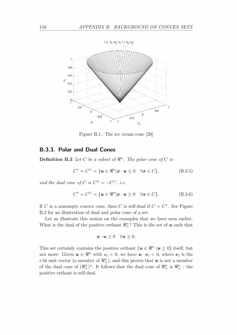
116 APPENDIX B. BACKGROUND ON CONVEX SETS
Figure B.1.: The ice cream cone [20]
B.3.3. Polar and Dual Cones
Definition B.3 Let C be a subset of <n. The polar cone of C is
C = C = u ∈ <n|x · u ≤ 0 ∀x ∈ C, (B.3.5)
and the dual cone of C is C⊕ = −C, i.e.
C∗ = C⊕ = u ∈ <n|x · u ≥ 0 ∀x ∈ C. (B.3.6)
If C is a nonempty convex cone, then C is self-dual if C = C∗. See Figure
B.2 for an illustration of dual and polar cone of a set.
Let us illustrate this notion on the examples that we have seen earlier.
What is the dual of the positive orthant <n+? This is the set of u such that
x · u ≥ 0 ∀x ≥ 0.
This set certainly contains the positive orthant u ∈ <n |u ≥ 0 itself, but
not more: Given u ∈ <n with ui < 0, we have u · ei < 0, where ei is the
i-th unit vector (a member of <n+), and this proves that u is not a member
of the dual cone of (<n+)∗. It follows that the dual cone of <n+ is <n+ : the
positive orthant is self-dual.

APPENDIX B. BACKGROUND ON CONVEX SETS 117
For the even more trivial cones, the situation is as follows.
C = 0 ⇒ C∗ = <n,C = <n ⇒ C∗ = 0.
Proposition B.1 The quadratic and rotated quadratic cone are self-dual
i.e.
(i) (Cq)∗ = Cq.
(ii) (Crq )∗ = Crq .
Proof 12 We first will show that the quadratic code is contained in the dual
cone. Since all vectors in the quadratic cone have first component nonnega-
tive we have:
z · x ≥ 0⇔ z1x1 ≥ −z2x2 − · · · − znxn
−z2x2 − · · · − znxn ≤ |(z2, · · · , zn) · (x2, · · · , xn)|= ‖(z2, · · · , zn)‖‖(x2, · · · , xn)‖|cos(θ)|≤ z1x1,
thus Cq ⊂ (Cq)∗. Next we show that the dual cone is contained in the
quadratic cone. If z ∈ (Cq)∗ then for all x ∈ C:
z1x1 ≥ −z2x2 − · · · − znxn= −(z2, · · · , zn) · (x2, · · · , xn)cos(θ)
= −‖(z2, · · · , zn)‖‖(x2, · · · , xn)‖cos(θ),now choose the member x∗ of C so that |x∗1| = 1, sign(x∗1) = sign(z1),
‖(x∗2, · · · , x∗n)‖ = 1 and cos(θ) = −1 then z1x1 = |z1| and we obtain:
|z1| ≥ ‖(z2, · · · , zn)‖,thus z ∈ Cq and (Cq)
∗ ⊂ Cq, Therefore (Cq)∗ = Cq.
(ii). In view of Remark B.2, since the rotated quadratic cone is identical
to the quadratic cone under a linear operator then is self-dual.
We conclude this section with the following intuitive fact: the dual of a
direct sum of cones is the direct sum of the dual cones. This fact is easy but
not entirely trivial. It actually requires a small proof, see [27].
Proposition B.2 Let K ⊂ <n, L ⊂ <m. Then
(K ⊕ L)∗ = K∗ ⊕ L∗.

118 APPENDIX B. BACKGROUND ON CONVEX SETS
(a) (b)
Figure B.2.: (a) A set C and its dual cone C∗, (b) A set C and its polar
cone C
B.4. Farkas Lemma, Cone Version
Under any meaningful notion of duality, you expect the dual of the dual
to be the primal (original) object. For cone duality (Definition B.3), this
indeed works.
Proposition B.3 Let K ⊂ <n be a closed convex cone. Then (K∗)∗ = K.
Maybe surprisingly, the proof of this innocent-looking fact already re-
quires the machinery of separation theorems that will also be essential for
cone programming duality below. Separation theorems generally assert that
disjoint convex sets can be separated by a hyperplane.
B.4.1. A Separation Theorem for Closed Convex Cones
Theorem B.1 Let K ⊂ <n be a closed convex cone, b ∈ <n\K. Then
there exists a vector y ∈ <n such that
y · x ≥ 0,∀x ∈ K, b · y < 0.
The statement is illustrated in Figure B.3 (left) for <2. The hyperplane
h = x ∈ <2|y · x = 0 (that passes through the origin) strictly separates b
from K. We also say that y is a witness for b /∈ K.

APPENDIX B. BACKGROUND ON CONVEX SETS 119
Proof 13 See [27].
Figure B.3.: A point b not contained in a closed convex cone K ⊂ <2 can
be separated from K by a hyperplane h = x ∈ <2|y · x = 0through the origin (left). The separating hyperplane resulting
from the proof of Theorem B.1(right).
Using this result, we can now show that (K∗)∗ = K for any closed convex
cone.
Proof of Proposition B.3.
For the directionK ⊂ (K∗)∗, we just need to apply the definition of
duality: Let us choose b ∈ K. By definition of K∗, y · b = b · y,∀y ∈K∗; this in turn shows that b ∈ (K∗)∗. For the other direction, we let
b /∈ K. According to Theorem B.1, we find a vector y such y · x ≥0,∀x ∈ K and b · y < 0. The former inequality shows that y ∈ K∗,but then the latter inequality witnesses that b /∈ (K∗)∗.
B.4.2. Adjoint Operators
We will now bring a linear operator into the game. Let V and W be
Hilbert spaces and let A : V → W be a linear operator from V into W . If
V and W are finite dimension, then A can be represented as a matrix. But
even in the general case, A behaves like a matrix for our purposes, and we
will write Ax instead of A(x) for x ∈ V . Here is the generalization of the
transpose of a matrix.

120 APPENDIX B. BACKGROUND ON CONVEX SETS
Definition B.4 Let A : V → W be a linear operator. A linear operator
AT : W → V is called an adjoint of A if
y ·Ax = ATy · x ∀x ∈ V,y ∈ W
If V and W are finite dimension, there is an adjoint AT of A. In general,
if there is an adjoint, then it is easy to see that it is unique which justifies
the notation AT .
In order to stay as close as possible to the familiar matrix terminol-
ogy, we will also introduce the following notation. If V1, V2, · · · , Vn and
W1,W2, · · · ,Wm are Hilbert spaces with linear operators Aij : Vj → Wi,
then we write the matrix
A11 A12 · · · A1n
A21 A22 · · · A2n...
.... . .
...
Am1 Am2 · · · Amn
(B.4.1)
for the linear operator A : V1⊕V2⊕· · ·⊕Vn → W1⊕W2⊕· · ·⊕Wm defined
by
A(x1,x2, · · · ,xn) = (
n∑
j=1
A1jxj ,
n∑
j=1
A2jxj , · · · ,n∑
j=1
Amjxj).
A simple calculation then shows that
AT =
AT11 AT
21 · · · ATm1
AT12 AT
22 · · · ATm2
......
. . ....
AT1n AT
2n · · · ATmn
(B.4.2)
just as with matrices.
Proposition B.4 Let A be a linear operator from <n into <m, and let C
be a nonempty closed convex cone in <m. Then the following hold :
(i) (A−1(C)) = AT (C).
(ii) (AT )−1(C) = (A(C)).
Proof 14 See [6].

APPENDIX B. BACKGROUND ON CONVEX SETS 121
B.4.3. Farkas Lemma
Proposition B.5 Let K ⊂ <n be a closed convex cone, and C = Ax|x ∈K. Then C, the closure of C, is a closed convex cone.
Proof 15 By definition, the closure of C is the set of all limit points of C.
Formally, b ∈ C if and only if there exists a sequence (yk)k ∈ N such that
yk ∈ C for all k and limk→∞ yk = b. This yields that C is a convex cone,
using that C is a convex cone. In addition, C is closed.
The fact b ∈ C can be formulated without reference to the cone C, and
this will be more convenient in what follows.
Definition B.5 Let K ⊂ <n be a closed convex cone. The system
Ax = b,x ∈ K,
is called subfeasible if there exists a sequence (xk)k∈N such that xk ∈ K for
all k ∈ N and
limk→∞
Ax = b.
Here is Farkas lemma for equation systems over closed convex cones.
Proposition B.6 Let K ⊂ <n be a closed convex cone, and b ∈ <m. The
system Ax = b,x ∈ K is subfeasible if and only if every y ∈ <m with
ATy ∈ K∗ also satisfies b · y ≥ 0.
Proof 16 See [27].


Bibliography
[1] E.D. Andersen, C. Roos, and T. Terlaky. On implementing a primal-
dual interior-point method for conic quadratic optimization, volume
95:249–277. 2003.
[2] MOSEK ApS. The mosek optimization tools version 3.2 (revision 8).
Avail. http://www.mosek.com, 2005.
[3] J.B. Baillon, R.E. Bruck, and S. Reich. On the asymptotic behavior of
nonexpansive mappings and semigroups in Banach spaces. Houston J.
Math., 4:1–9, 1978.
[4] H.H. Bauschke and J.M. Borwein. On the convergence of von Neumanns
alternating projection algorithm for two sets. Set-Valued. Anal., 1:185–
212, 1993.
[5] H.H. Bauschke and J.M. Borwein. On projection algorithms for solving
convex feasibility problems. SIAM Review., 38:367–426, 1996.
[6] H.H. Bauschke and P.L. Combettes. Convex analysis and monotone
operator theory in Hilbert spaces. Springer, 2010.
[7] H.H. Bauschke, P.L. Combettes, and D. Russel Lukel. Finding best
approximation pairs relative to two closed convex sets in Hilbert spaces.
J. Approx. Theory., 127:178–192, 2004.
[8] D.P. Bertsekas. Nonlinear programming. Athena Scientific, second edi-
tion, 1999.
123

124 Bibliography
[9] D.P. Bertsekas. Convex analysis and optimization. Athena Scientific,
2003.
[10] D.P. Bertsekas and Tsitsiklis. Parallel and Distributed Computation:
Numerical Methods. Prentice Hall, New York, 1989.
[11] S. Boyd and L. Vandenberghe. Convex optimisation. Cambridge Uni-
versity Press, 2004.
[12] R.E. Bruck and S. Reich. Nonexpansive projections and resolvents of
accretive operators in Banach spaces. Houston J. Math., 3:459–470,
1977.
[13] G. Chen and M. Teboulle. A proximal-based decomposition method for
convex minimization problems. Math. Progr. Ser. A, 64:81–101, 1994.
[14] W.F. Chen. Limit analysis in soil mechanics. Elsevier, 1990.
[15] E. Christiansen. Handbook of Numerical Analysis, volume IV, chapter
Limit Analysis of Collapse States. North Holland Amsterdam, 1996.
[16] H. Ciria. Computational of upper and lower bounds in limit analysis
using second cone programming and mesh adaptivity, May 14 2004.
MSc thesis.
[17] P.L. Combettes. Inconsistent signal feasibility problems: least-squares
solutions in a product space. IEEE Trans. Signal Process., 42:2955–
2966, 1994.
[18] P.L. Combettes. Hilbertian convex feasibility problem: convergence of
projection methods. Appl. Mathl. Optim, 35:311–330, 1997.
[19] A.J. Conejo, E. Castillo, R.Mınguez, and R. Garcıa-Bertrand. Decom-
position Techniques in Mathematical Programming. Springer, 2006.
[20] G. Cornuejols and R. Tutuncu. Optimisation methods in finace. Cam-
bridge, 2007.
[21] M. Vicente da Silva and A.N. Antao. A non-linear programming method
approch for upper bound limit analysis. Int. J. Numer. Meth. Eng.,
72:1192–1218, 2007.

Bibliography 125
[22] M. Vicente da Silva and A.N. Antao. Upper bound limit analysis with a
parallel mixed fnite element formulation. Int. J. Solids Struct., 45:5788–
5804, 2008.
[23] G.B. Dantzig and P. Wolfe. Decomposition principle for linear pro-
gramming. Math. Oper. Res., 8:101–111, 1960.
[24] F. Deutsch. Best Approximation in Inner Product Spaces. Springer,
2001.
[25] Q.T. Dinh, C. Savorgnan, and M. Diehl. Combining Lagrangian decom-
position and excessive gap smoothing technique for solving larg-escale
separable convex optimization problems. Comput. Optim. Appl., 55:75–
111, 2013.
[26] S.A. Gabriel, Y. Shim, A.J. Conejo, S. de la Torre, and R. Garca-
Bertrand. A Benders decomposition method for discretely-constrained
mathematical programs with equilibrium constraints. J. Oper. Res.
Soc. , 61(9):1404–1419, 2010.
[27] B. Gartner and J. Matousek. Approximation Algorithms and Semidef-
inite Programming. Springer, 2012.
[28] M. Goldburg and R.J. Marks II. Signal synthesis in the presence of an
inconsistent set of constraints. IEEE Trans. Circuits Syst., 32:647–663,
1985.
[29] J. Huang, W. Xu, P. Thomson, and S. Di. A general rigid-plastic/rigid-
viscoplastic FEM for metal-forming processes based on the potential
reduction interior point method. Int. J. Mach. Tool. Manuf., 43:379–
389, 2003.
[30] I. Kaneko. A decomposition procedure for large-scale optimum plastic
design problems. Int. J. Numer. Meth. Eng., 19:873–889, 1983.
[31] K. Krabbenhøft, A.V. Lyamin, and S.W. Sloan. Formulation and so-
lution of some plasticity problems as conic programs. Int. J. Solids
Struct., 44:1533–1549, 2007.
[32] A.V. Lyamin. Sonic. Solver for second order conic programing. 2004.

126 Bibliography
[33] A.V. Lyamin and S.W. Sloan. Lower bound limit analysis using non-
linear programming. Int. J. Numer. Meth. Eng., 55:576–611, 2002.
[34] A.V. Lyamin, S.W. Sloan, K. Krabbenhft K, and M. Hjiaj. Lower
bound limit analysis with adaptive remeshing. Int. J. Numer. Meth.
Eng., 63:1961–1974, 2005.
[35] A. Makrodimopoulos and C.M. Martin. Lower bound limit analysis of
cohesive-frictional materials using second-order cone programming. Int.
J. Numer. Meth. Eng., 66:604–634, 2006.
[36] R.D.C. Monteiro, C. Ortiz, and B.F. Svaiter. Implementation of a
block-decomposition algorithm for solving large-scale conic semidefinite
programming problems. Comput. Optim. Appl., 2013.
[37] J.J. Munoz, J. Bonet, A. Huerta, and J. Peraire. Upper and lower
bounds in limit analysis: adaptive meshing strategies and discontinuous
loading. Int. J. Numer. Meth. Eng., 77:471–501, 2009.
[38] I. Necoara and J.A.K. Suyken. Application of a smoothing technique
to decomposition in convex optimization. IEEE. T. Automat. Contr.,
pages 2674–3679, 2008.
[39] Y. Nesterov. Smooth minimization of non-smooth functions. Math.
Progr. Ser. A, 103(1):127–152, 2005.
[40] Z. Opial. Weak convergence of the sequence of successive approxima-
tions for nonexpansive mappings. Bull. Amer. Math. Soc., 73:591–597,
1967.
[41] F. Pastor, E. Loute, J. Pastor, and M. Trillat. Mixed method and con-
vex optimization for limit analysis of homogeneous Gurson materials:
a kinematical approach. Eur. J. Mech. A/Solids, (28):25–35, 2009.
[42] A. Pazy. Asymptotic behavior of contractions in Hilbert space. Israel.
J. Math., 9:235–240, 1971.
[43] J.C. Pesquet and P.L. Combettes. Wavelet synthesis by alternating
projections. IEEE Trans. Signal Process., 44:728–732, 1996.

Bibliography 127
[44] R.L. Raffard, C.J. Tomlin, and S.P. Boyd. Distributed optimization for
cooperative agents, application to formation flight. 43rd IEEE Confer-
ence on Decision and Contro, December 2004.
[45] J. F. Sturm. Using SeDuMi 1.02, a MATLAB toolbox for optimization
over symmetric cones. Optim. Method. Softw, 11–12:625–653, 1999.
Version 1.05 available from http://http://sedumi.ie.lehigh.edu.
[46] K.C. Toh, M.J. Todd, and R.H. Tutuncu. On the implementation and
usage of SDPT3 a Matlab software package for semidefinite-quadratic
linear programming. Version 4.0. Technical report,National University
of Singapore, july 2006.
[47] R.H. Tutuncu, K.C. Toh, and M.J. Todd. Solving semidefinite-
quadratic-linear programs using SDPT3. MPB, 95:189–217, 2003.
Avail. http://www.math.nus.edu.sg/ mattohkc/sdpt3.html.