decompression wave speed in co2 mixtures: cfd modelling
TRANSCRIPT

University of Wollongong University of Wollongong
Research Online Research Online
Faculty of Engineering and Information Sciences - Papers: Part A
Faculty of Engineering and Information Sciences
31-12-2014
Decompression wave speed in CO2 mixtures: CFD modelling with the Decompression wave speed in CO2 mixtures: CFD modelling with the
GERG-2008 equation of state GERG-2008 equation of state
Alhoush Elshahomi University of Wollongong, [email protected]
Cheng Lu University of Wollongong, [email protected]
Guillaume Michal University of Wollongong, [email protected]
Xiong Liu University of Wollongong, [email protected]
Ajit R. Godbole University of Wollongong, [email protected]
See next page for additional authors
Follow this and additional works at: https://ro.uow.edu.au/eispapers
Part of the Engineering Commons, and the Science and Technology Studies Commons
Recommended Citation Recommended Citation Elshahomi, Alhoush; Lu, Cheng; Michal, Guillaume; Liu, Xiong; Godbole, Ajit R.; and Venton, Phillip, "Decompression wave speed in CO2 mixtures: CFD modelling with the GERG-2008 equation of state" (2014). Faculty of Engineering and Information Sciences - Papers: Part A. 3310. https://ro.uow.edu.au/eispapers/3310
Research Online is the open access institutional repository for the University of Wollongong. For further information contact the UOW Library: [email protected]
Decompression wave speed in CO2 mixtures: CFD modelling with the GERG-2008 Decompression wave speed in CO2 mixtures: CFD modelling with the GERG-2008 equation of state equation of state
Abstract Abstract The development of CO2 pipelines for Carbon Capture and Storage (CCS) raises new questions regarding the control of ductile fracture propagation and fracture arrest toughness criteria. The decompression behaviour in the fluid must be determined accurately in order to estimate the proper pipe toughness. However, anthropogenic CO2 may contain impurities that can modify the fluid decompression characteristics quite significantly. To determine the decompression wave speed in CO2 mixtures, the thermodynamic properties of these mixtures must be determined by using an accurate equation of state. In this paper we present a new decompression model developed using the Computational Fluid Dynamics (CFD) package ANSYS Fluent. The GERG-2008 Equation of State (EOS) was implemented into this model through User Defined Functions (UDF) to predict the thermodynamic properties of CO2 mixtures. The model predictions were in good agreement with the experimental data of two 'shock tube' tests. A range of representative CO2 mixtures was examined in terms of the changes in fluid properties from the initial conditions, with time and distance, immediately after a sudden pipeline opening at one end. Phase changes that may occur within the fluid due to condensation of 'impurities' in the fluid were also investigated. Simulations were also conducted to examine how the initial temperature and impurities would affect the decompression wave speed.
Keywords Keywords CO2 pipeline, decompression wave speed, equation of state, computational fluid dynamics, fracture propagation arrest
Disciplines Disciplines Engineering | Science and Technology Studies
Publication Details Publication Details Elshahomi, A., Lu, C., Michal, G., Liu, X., Godbole, A. & Venton, P. (2015). Decompression wave speed in CO2 mixtures: CFD modelling with the GERG-2008 equation of state. Applied Energy, 140 20-32.
Authors Authors Alhoush Elshahomi, Cheng Lu, Guillaume Michal, Xiong Liu, Ajit R. Godbole, and Phillip Venton
This journal article is available at Research Online: https://ro.uow.edu.au/eispapers/3310
Decompression wave speed in CO2 mixtures: CFD modelling with the
GERG-2008 equation of state
Alhoush Elshahomia, Cheng Lua*, Guillaume Michala, Xiong Liua, Ajit Godbolea, Philip Ventonb
a School of Mechanical, Materials and Mechatronic Engineering, University of Wollongong,
Wollongong, NSW 2522, Australia
b Venton and Associates Pty Ltd, Bundanoon, NSW 2578, Australia
Abstract
The development of CO2 pipelines for Carbon Capture and Storage (CCS) raises new questions
regarding the control of ductile fracture propagation and fracture arrest toughness criteria. The
decompression behaviour in the fluid must be determined accurately in order to estimate the proper
pipe toughness. However, anthropogenic CO2 may contain impurities that can modify the fluid
decompression characteristics quite significantly. To determine the decompression wave speed in CO2
mixtures, the thermodynamic properties of these mixtures must be determined by using an accurate
equation of state. In this paper we present a new decompression model developed using the
Computational Fluid Dynamics (CFD) package ANSYS Fluent. The GERG-2008 Equation of State
(EOS) was implemented into this model through User Defined Functions (UDF) to predict the
thermodynamic properties of CO2 mixtures. The model predictions were in good agreement with the
experimental data of two ‘shock tube’ tests. A range of representative CO2 mixtures was examined in
terms of the changes in fluid properties from the initial conditions, with time and distance,
immediately after a sudden pipeline opening at one end. Phase changes that may occur within the
fluid due to condensation of ‘impurities’ in the fluid were also investigated. Simulations were also
conducted to examine how the initial temperature and impurities would affect the decompression
wave speed.
Keywords: CO2 pipeline; decompression wave speed; equation of state; computational fluid
dynamics; fracture propagation arrest
* Corresponding author. Tel.: +61-2-4221-4639; Fax: +61-2-4221-5474.
E-mail address: [email protected] (C. Lu).
Nomenclature
c Speed of sound (m s-1)
E Fluid energy (kJ)
h Enthalpy (kJ kg-1)
M Molecular weight (kg)
p Pressure (Pa)
s Entropy (kJ kg-1 K-1)
t Time (s)
T Temperature (K)
u Outflow velocity (m s-1)
Pi Initial pressure (Pa)
Ti Initial temperature (K)
Vc Fracture velocity (m s-1)
Wave Average decompression wave speed (m s-1)
Wexp Measured decompression wave speed (m s-1)
Wlocal Local decompression wave speed (m s-1)
keff Effective thermal conductivity (W m-1 K-1)
cp Specific Heat (kJ kg-1 K-1)
ρ Fluid density(kg m-3)
vx Axial velocity (m s-1)
vy Radial velocity (m s-1)
µ Dynamic viscosity (Pa s)
Abbreviations
2D Two-dimensional
AGA American Gas Association
AS Australian Standard
AUSM Advection upstream splitting method
BTCM Battelle Two-Curve Model
BWRS Benedict-Webb-Rubin-Starling
CCS Carbon Capture and Storage
CFD Computational fluid dynamics
CO2 Carbon dioxide
CVN Charpy V-Notch
EOS Equation of State
FDM Finite Difference Method
FVM Finite Volume Method
GERG Groupe Européen de Recherches Gazières
GHG Green House Gases
ID Internal Diameter
UDF User Defined Functions
MOC Method of Characteristics
PR Peng-Robinson
RKS Redlich-Kwong-Soave
1. Introduction
The burning of fossil fuels and biomass continues to be the main source of energy worldwide [1, 2].
Such processes emit significant quantities of Green House Gases (GHG), particularly Carbon Dioxide
(CO2), which has been identified as the major contributor to global warming and climate change [3,
4]. Carbon Capture and Storage (CCS) technology was introduced as a key CO2 abatement option to
mitigate emissions of GHG by 50% by 2050, while populations and economies are expected to
continue to grow globally [5]. This technology will necessitate substantial quantities of CO2 to be
conveyed, predominantly by pipelines, over long distances from source to storage sites [6]. In terms
of operational and economic motivations, the best way to transport CO2 mixtures via pipes will be in

a liquid and/or supercritical state because a purely gaseous phase transmission would necessitate
significantly larger diameter pipelines for the same mass flow rate [7, 8]. Under these operational
conditions, the possibility of running fractures in the pipeline is a major concern, so arresting and/or
preventing them is important for the integrity and safety of the pipeline’s operation [5, 7].
Fracture propagation in gas pipelines is commonly treated using the semi-empirical Battelle Two-
Curve Model (BTCM) [9, 10] where the aim is to estimate the required toughness to arrest crack
propagation. This method involves the superposition of two independently determined curves: the
fluid decompression wave speed and the fracture propagation speed (the ‘J curve’), each expressed as
a function of pressure. Fig. 1 shows a schematic representation of the BTCM. The shape of the fluid
decompression wave speed curve depends on the phase of the fluid, as shown by the red and green
curves in Fig. 1. Curves 1, 2, and 3 represent the fracture speed curves for different toughness values.
Fig. 1. Schematic of the BTCM [11]
When fracture curves 2 and 3 intersect with the two-phase decompression characteristic, the fracture
and the gas decompression wave move at the same speed, but here the gas pressure at the tip of the
fracture no longer decreases, implying that the fracture will continue to propagate. The boundary

between arrest and propagation of a running fracture is represented by tangency between the gas
decompression wave speed curve and the fracture speed curve (curve 1 with the two-phase
decompression wave speed curve and curve 3 with the single phase decompression wave speed
curve). According to the BTCM, the minimum toughness required to arrest the propagation of fracture
is the value of toughness corresponding to this tangency condition [9, 11].
Several numerical models have been proposed to predict the decompression wave speed, mainly in
natural gas mixtures. One of these models is GASDECOM [12]. This model uses an analytical
expression for the propagation of an infinitesimal decompression front to determine the
decompression wave speed. The main assumptions in such models include: one-dimensional,
frictionless, isentropic, and homogeneous-equilibrium fluid flow. GASDECOM uses the Benedict-
Webb-Rubin-Starling (BWRS) Equation of State (EOS) [13] with modified constants to estimate the
thermodynamic properties during isentropic decompression. GASDECOM has suffered from
numerical instabilities when dealing with mixtures containing higher fractions of CO2. It should be
mentioned that the instabilities are due to the implementation in the code, and are not fundamental.
GASDECOM cannot be used for mixtures containing hydrogen, oxygen and argon, which are often
mixed with CO2 in CCS-related operations. This is because these components were not originally
included in the BWRS EOS [14, 15]. Several other models also use assumptions similar to
GASDECOM [16], and only differ in the choice of EOS. DECOM [17] was developed to predict the
decompression wave speed in CO2 mixtures, and is also based on assumptions similar to those in
GASDECOM. The only difference was use of the NIST Standard Reference Database 23 (REFPROP
version 9.0) [18], along with the built-in Span and Wagner EOS [19] for pure CO2 and the GERG-
2004 EOS [20] for multi-component CO2 mixtures.
Other more complex decompression models that can account for non-isentropic effects using the
Computational Fluid Dynamics (CFD) technique have been developed. Examples include: Picard and
Bishnoi [21, 22], PipeTech [23, 24] and CFD-DECOM [25]. These are based entirely on assumptions
of one-dimensional homogeneous-equilibrium fluid flow. In these models the effects of friction, heat
transfer, and pipe diameter can be considered, which is particularly relevant for smaller diameter and
longer pipelines where friction could lead to a range of complex effects on local flow conditions,
temperature, and pressure within the pipeline [24, 26-29]. CFD-based techniques involve discretising
the governing partial differential equations of fluid flow. The Finite Difference Method FDM [30, 31],
the Method Of Characteristics (MOC) [32], and the Finite Volume Method (FVM) [25] are examples
of discretisation methods. The MOC solves the fluid flow conservation equations by following the
Mach-line characteristics inside the pipe. It is claimed that numerical diffusion related to the finite
difference approximation of partial derivatives is reduced by this method [33, 34], but the MOC needs
much longer computation runtimes and cannot predict non-equilibrium or heterogeneous flows [25,
35], while the FVM is better at dealing with multi-dimensional flow. In the existing CFD models, the
cubic Peng-Robinson (PR) EOS [36] is often used due to its relatively simple mathematical form
compared to other more complex (but more accurate) EOS such as AGA-8 [37], BWRS [13] and
GERG[20].
To accurately predict the decompression behaviour of CO2 mixtures, accurate means of predicting the
thermodynamic properties of these mixtures using accurate EOS is essential. To date, no EOS is
specifically recommended for CO2 mixtures, but the ability to accurately predict the Vapour Liquid
Equilibrium (VLE), density and speed of sound is considered the best way to gauge any weaknesses
or strengths of EOS [2, 8, 38, 39]. Li et al. [2, 8] have evaluated eight cubic EOS, including Peng–
Robinson (PR) [36], Patel–Teja (PT) [40], Redlich–Kwong (RK) [41], Redlich–Kwong–Soave (SRK)
[42], modified SRK (MRK) [43], modified PR (MPR) [44], 3P1T EOS [45], and Improved SRK
(ISRK) [46], in terms of predicting the VLE and specific volumes of binary CO2 mixtures containing
CH4, H2S, SO2, Ar and N2, based on the comparisons with experimental data. Generally, PR is
recommended for calculations involving CO2/CH4 and CO2/H2S; PT is recommended for CO2/O2,
CO2/N2 and CO2/Ar; 3P1T is recommended for CO2/SO2. Liu et al. [47] have implemented the PR
EOS into ANSYS Fluent using real gas User-Defined Functions (UDFs) in order to simulate the
dispersion of pure CO2 releases from high-pressure pipelines. Reasonable results were obtained when
using the real gas models in conjunction with the CFD method. Botros [48, 49] conducted a

comparative study of five different EOSs: GERG, AGA-8, BWRS, PR and Redlich-Kwong-Soave
(RKS) and compared the predicted densities in the dense phase region using those EOS with
measured values for different hydrocarbon mixtures. It was determined that the GERG EOS
outperformed the other EOS in the region up to P = 30 MPa and T > -8 °C. However, the GERG EOS
has not been implemented in CFD models of decompression or outflow models to date , though it is
currently the reference EOS for natural gas [50].
In this paper we present a CFD model for a full-bore depressurisation of a CO2 mixture pipeline
developed using the versatile CFD software ANSYS Fluent (v 14.5). The built-in EOS in ANSYS
Fluent cannot predict the fluid properties of CO2 mixtures accurately. The GERG-2008 EOS was
successfully implemented into ANSYS Fluent to accurately predict the thermodynamic properties of
CO2 mixtures, for the first time. The method used to implement the GERG-2008 EOS into ANSYS
Fluent is described. The results were validated against experimental data from two separate ‘shock
tube’ tests, and a number of simulations were also conducted to examine the effect of different initial
conditions and different components in the CO2 mixture.
2. Methodology
The CFD package ANSYS-Fluent was used to develop the CFD decompression model because it
satisfies the three main demands required for gas decompression analysis:
Ability to solve transient flows;
Possibility of invoking an accurate EOS through user-defined subroutines;
Ability to handle multi-dimensional geometries.
2.1. Computational domain and boundary conditions
The physical flow domain in the shock tube tests consisted of the initially pressurised gas in a
horizontal pipe, which undergoes a ‘full-bore’ opening at one end using a rupture disc as

schematically depicted in Fig. 2. The axial symmetry made it possible to construct a two-dimensional
computational domain and thus reduce the computational runtime.
Fig. 2. Flow domain and computational domain – schematic
The following assumptions are made to develop this model: unsteady, two-dimensional flow; the
rupture is instantaneous and represented by a full bore opening, non-isentropic flow conditions (the
friction effect is considered); the gas velocity before the rupture of the pipe is negligible compared
with the conditions post-rupture; the fluid is considered homogenous so equilibrium conditions
prevail during condensation; and the ‘no slip’ condition is satisfied at the pipe wall.
Four boundary conditions were defined: two ‘wall’ boundaries defined at the top (y = D/2) and the
end (x = L) of the computational domain; a ‘symmetry’ boundary (at y = 0) on the axis and a pressure
outlet (zero gauge pressure) to model the rupture disk (sudden opening to the ambient) at x = 0. Based
on the above assumptions, the unsteady, two-dimensional form of the governing differential equations
of conservation of mass, momentum and energy are solved in this model.
2.2. Numerical Method
The FVM is used in ANSYS Fluent to discretise the fluid conservation equations. The implicit first
order spatial and temporal formulations were used with the Advection Upstream Splitting Method
(AUSM) for the density-based solver [51]. This solver is designed for high-speed compressible flows
and allows the use of a user defined real gas model. The governing flow equations of mass,
momentum, and energy conservation, supplemented by the auxiliary equation (i.e. EOS) were solved
simultaneously while the turbulence equations were treated sequentially. In the density-based solver,
the momentum equations were used to obtain the velocity field, while the continuity equation was
used to determine the density field and the pressure field was determined from the EOS.
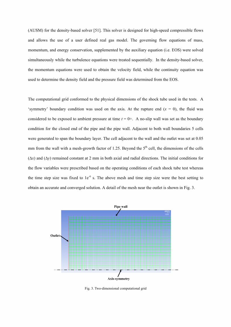
The computational grid conformed to the physical dimensions of the shock tube used in the tests. A
‘symmetry’ boundary condition was used on the axis. At the rupture end (x = 0), the fluid was
considered to be exposed to ambient pressure at time t = 0+. A no-slip wall was set as the boundary
condition for the closed end of the pipe and the pipe wall. Adjacent to both wall boundaries 5 cells
were generated to span the boundary layer. The cell adjacent to the wall and the outlet was set at 0.05
mm from the wall with a mesh-growth factor of 1.25. Beyond the 5th cell, the dimensions of the cells
(∆x) and (∆y) remained constant at 2 mm in both axial and radial directions. The initial conditions for
the flow variables were prescribed based on the operating conditions of each shock tube test whereas
the time step size was fixed to 1e-6 s. The above mesh and time step size were the best setting to
obtain an accurate and converged solution. A detail of the mesh near the outlet is shown in Fig. 3.
Fig. 3. Two-dimensional computational grid

The speed of the decompression wave was obtained by first calculating the local decompression wave
speed using Eq. (1), i.e., by monitoring the speed of sound ‘c’ and the ‘outflow’ velocity ‘u’ against
time during the decompression process. The decompression wave speed was then determined by
subtracting the outflow velocity from the speed of sound for several pressures below the initial
pressure.
ucWlocal (1)
However, experimental tests such as the shock tube test did not provide the local gas decompression
wave speed directly because the gas decompression wave speed w was calculated by determining the
times at which a certain pressure level was recorded at several pressure transducers at known
locations on the pipe wall. By plotting these locations against time, the decompression wave speed
was obtained by performing a linear regression of each isobar curve. The slope of each regression
represents the average decompression wave speed for each isobar.
dt
dxWave (2)
3. Implementation of GERG-2008 EOS into ANSYS Fluent
To simulate the real behaviour of gas flow, the thermodynamic properties must be predicted using an
accurate real gas EOS. The modern multi-component GERG-2008 EOS [20, 52] was used to provide
the thermodynamic properties of CO2 mixtures. This EOS covers the gas phase, liquid phase,
supercritical region, and vapour-liquid equilibrium states for mixtures consisting of up to 21
components: methane, nitrogen, carbon dioxide, ethane, propane, n-butane, isobutane, n-pentane,
isopentane, n-hexane, n-heptane, n-octane, hydrogen, oxygen, carbon monoxide, water, helium,
argon, n-nonane, n-decane, and hydrogen sulphide. The normal range of validity of this EOS covers
temperatures from 90 K to 450 K and pressures up to 35 MPa. Currently, GERG-2008 EOS is
considered to be a reference EOS for natural gas pipelines [14].
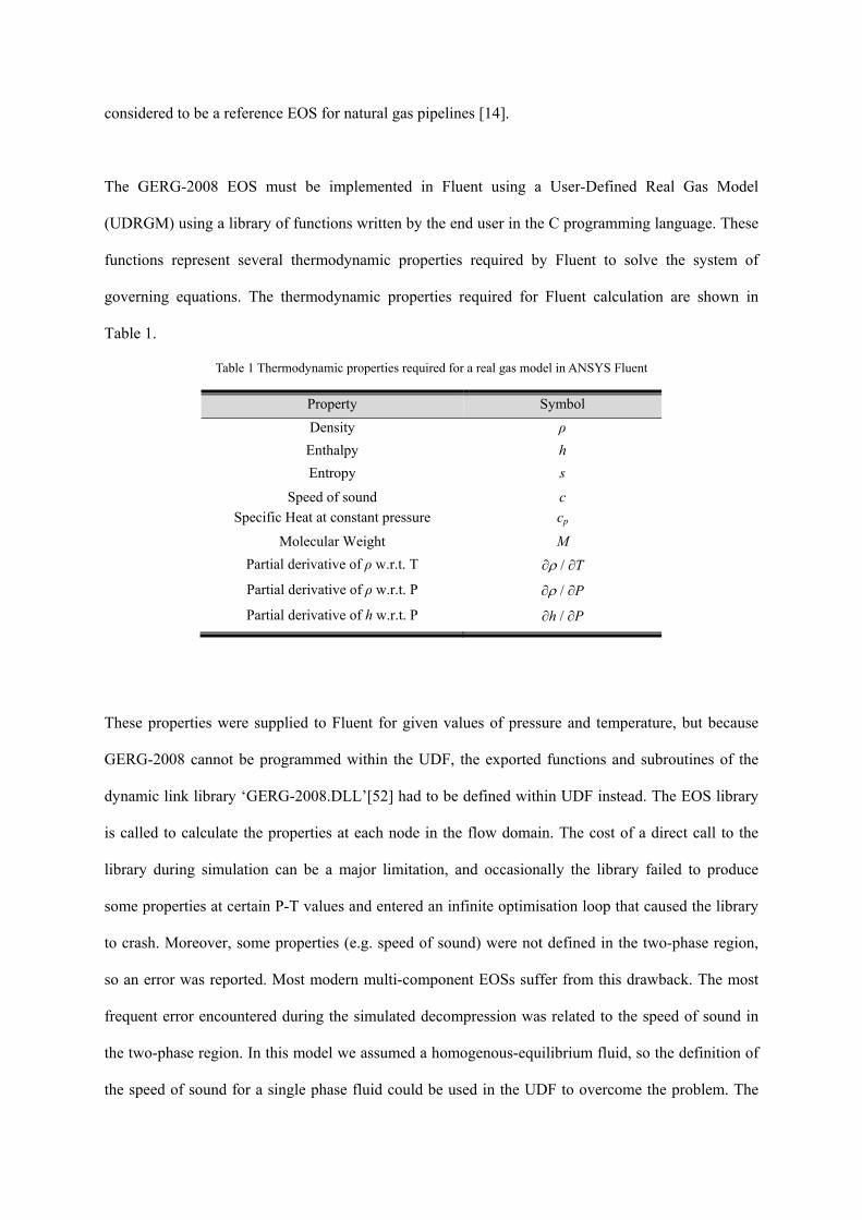
The GERG-2008 EOS must be implemented in Fluent using a User-Defined Real Gas Model
(UDRGM) using a library of functions written by the end user in the C programming language. These
functions represent several thermodynamic properties required by Fluent to solve the system of
governing equations. The thermodynamic properties required for Fluent calculation are shown in
Table 1.
Table 1 Thermodynamic properties required for a real gas model in ANSYS Fluent
Property Symbol
Density ρ
Enthalpy h
Entropy s
Speed of sound c
Specific Heat at constant pressure cp
Molecular Weight M
Partial derivative of ρ w.r.t. T ∂/ ∂T
Partial derivative of ρ w.r.t. P ∂/ ∂P
Partial derivative of h w.r.t. P ∂h/ ∂P
These properties were supplied to Fluent for given values of pressure and temperature, but because
GERG-2008 cannot be programmed within the UDF, the exported functions and subroutines of the
dynamic link library ‘GERG-2008.DLL’[52] had to be defined within UDF instead. The EOS library
is called to calculate the properties at each node in the flow domain. The cost of a direct call to the
library during simulation can be a major limitation, and occasionally the library failed to produce
some properties at certain P-T values and entered an infinite optimisation loop that caused the library
to crash. Moreover, some properties (e.g. speed of sound) were not defined in the two-phase region,
so an error was reported. Most modern multi-component EOSs suffer from this drawback. The most
frequent error encountered during the simulated decompression was related to the speed of sound in
the two-phase region. In this model we assumed a homogenous-equilibrium fluid, so the definition of
the speed of sound for a single phase fluid could be used in the UDF to overcome the problem. The
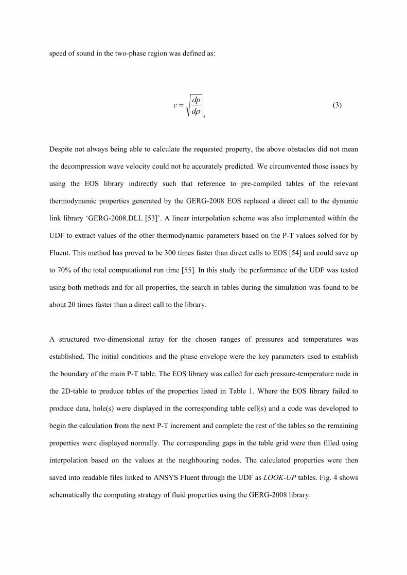
speed of sound in the two-phase region was defined as:
sd
dpc
(3)
Despite not always being able to calculate the requested property, the above obstacles did not mean
the decompression wave velocity could not be accurately predicted. We circumvented those issues by
using the EOS library indirectly such that reference to pre-compiled tables of the relevant
thermodynamic properties generated by the GERG-2008 EOS replaced a direct call to the dynamic
link library ‘GERG-2008.DLL [53]’. A linear interpolation scheme was also implemented within the
UDF to extract values of the other thermodynamic parameters based on the P-T values solved for by
Fluent. This method has proved to be 300 times faster than direct calls to EOS [54] and could save up
to 70% of the total computational run time [55]. In this study the performance of the UDF was tested
using both methods and for all properties, the search in tables during the simulation was found to be
about 20 times faster than a direct call to the library.
A structured two-dimensional array for the chosen ranges of pressures and temperatures was
established. The initial conditions and the phase envelope were the key parameters used to establish
the boundary of the main P-T table. The EOS library was called for each pressure-temperature node in
the 2D-table to produce tables of the properties listed in Table 1. Where the EOS library failed to
produce data, hole(s) were displayed in the corresponding table cell(s) and a code was developed to
begin the calculation from the next P-T increment and complete the rest of the tables so the remaining
properties were displayed normally. The corresponding gaps in the table grid were then filled using
interpolation based on the values at the neighbouring nodes. The calculated properties were then
saved into readable files linked to ANSYS Fluent through the UDF as LOOK-UP tables. Fig. 4 shows
schematically the computing strategy of fluid properties using the GERG-2008 library.

4. Mode
The foll
2008 EO
tests. Th
el results an
lowing parag
OS. This mo
he first test (
NO
In
Se
C(ρ, h,
For the tw
C
d validation
graphs presen
odel was val
(Case A) was
S
nput the mixtu
et Pmin, Tmin, P
Calccom
Plot pha
Call GERG-li, s, cp, M, c, dρ
wo-phase regio
Library cr
Calculate from
Calccom
Fig. 4. Prop
n
nt the results
lidated by a
s conducted
NO
Start
ure compositio
max, Tmax, ∆P &
culation mpleted?
ase envelope
brary to calcudρ/dT, dρ/dp &
on calculate c
rash detected
m next P-T inte
culation mpleted?
perty calculatio
s of the 2D C
comparison
at the Trans
YES
on, Pi & Ti
& ∆T
ulate & dh/dP)
using Eq. (3)
erval
on flow chart
CFD decomp
with the re
sCanada pipe
YES
Save
Loc
Deter
pression mod
sults of two
eline Gas Dy
e properties in
cate missing p
End
rmine missingusing interpo
del using the
o separate sh
ynamics Test
nto txt-files
properties
g properties olation
e GERG-
hock tube
t Facility

in Didsbury, Alberta, Canada [56]. The second test (Case B) was commissioned by the National Grid
at GL Noble Denton’s Spadeadam Test Site in Cumbria, UK [17]. In the first test, the main section of
the shock tube was 42 m long, the internal diameter (ID) was 38.1 mm and the tube wall thickness
was 11.1 mm. In the second test the pipe was 144 m long, the ID was 146.36 mm, and the pipe wall
thickness was 10.97 mm. In Case A, a ‘smooth’ pipe surface was used, while in Case B the pipe has
an average surface roughness ranging between 5 and 6.3µm. The smoothest pipe was placed nearest
the rupture disk. Table 2 lists model parameters used in the current simulations.
Table 2 Model parameters setting for the current study
Case Pipe length
(m) Diameter
(mm) Surface
roughness(µm) Turbulence
model
Case A 42 38.1 Smooth Realisable k-ɛ
Case B 144 146.36 5 Realisable k-ɛ
CFD simulations were carried out for two mixtures: a binary mixture for Case A and a 5-component
mixture for Case B. Table 3 shows the gas compositions and initial conditions of the two tests.
Table 3 Mixture composition and initial conditions of shock tube tests
Shock Tube Test
Mixture components (mole %) Pi (MPa) Ti (K) CO2 H2 N2 O2 CH4
Case A 72.6 0 0 0 27.4 28.568 313.65
Case B (T31) 91.03 1.15 4 1.87 1.95 14.95 283.15
A mesh-dependence study was carried out for both cases using several element sizes (2, 3, 5, 10, 20,
50, 100 mm). An optimum element size was found to be 2mm, although for decompression wave
speed calculation, an element size up to 10 mm was found acceptable.
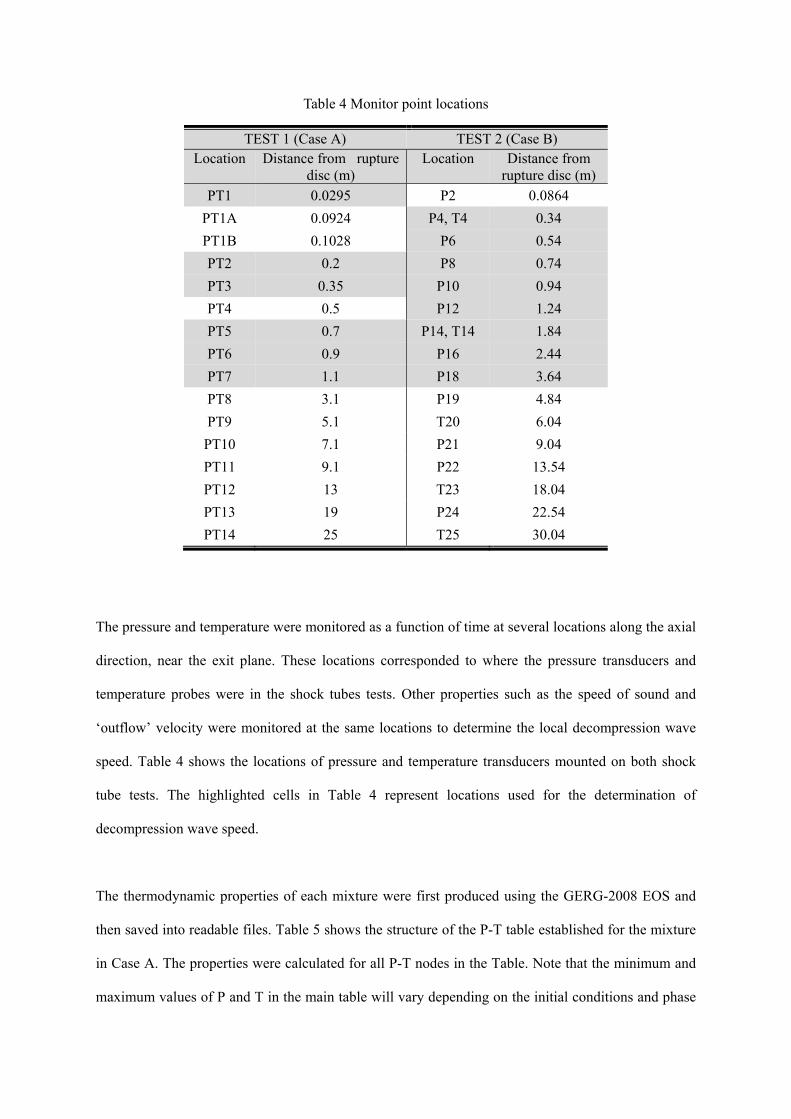
Table 4 Monitor point locations
TEST 1 (Case A) TEST 2 (Case B) Location Distance from rupture
disc (m) Location Distance from
rupture disc (m)
PT1 0.0295 P2 0.0864
PT1A 0.0924 P4, T4 0.34
PT1B 0.1028 P6 0.54
PT2 0.2 P8 0.74
PT3 0.35 P10 0.94
PT4 0.5 P12 1.24
PT5 0.7 P14, T14 1.84
PT6 0.9 P16 2.44
PT7 1.1 P18 3.64
PT8 3.1 P19 4.84
PT9 5.1 T20 6.04
PT10 7.1 P21 9.04
PT11 9.1 P22 13.54
PT12 13 T23 18.04
PT13 19 P24 22.54
PT14 25 T25 30.04
The pressure and temperature were monitored as a function of time at several locations along the axial
direction, near the exit plane. These locations corresponded to where the pressure transducers and
temperature probes were in the shock tubes tests. Other properties such as the speed of sound and
‘outflow’ velocity were monitored at the same locations to determine the local decompression wave
speed. Table 4 shows the locations of pressure and temperature transducers mounted on both shock
tube tests. The highlighted cells in Table 4 represent locations used for the determination of
decompression wave speed.
The thermodynamic properties of each mixture were first produced using the GERG-2008 EOS and
then saved into readable files. Table 5 shows the structure of the P-T table established for the mixture
in Case A. The properties were calculated for all P-T nodes in the Table. Note that the minimum and
maximum values of P and T in the main table will vary depending on the initial conditions and phase

envelope of each mixture.
Table 5 P-T table
Pressure (MPa) Temperature (K)
Min 0.05 180
Max 30 320
Increment 0. 1 0.5
No. of nodes 300 281
A MATLAB code was written to generate plots of the required properties as a function of pressure
and temperature. The calculated properties for Case A are presented in Fig. 5. A smooth distribution
was observed for all properties, including the region under the two-phase boundary. This occurred
because the main P-T table was made dense enough to account for changes near the phase boundary.
This makes for very large files, but it ensured that the calculations were accurate. An acceptable
accuracy was achieved using the property tables: the interpolated properties deviated from values
obtained directly using the EOS library by approximately 0.001% outside the two-phase region, and
0.1% within the two-phase region.
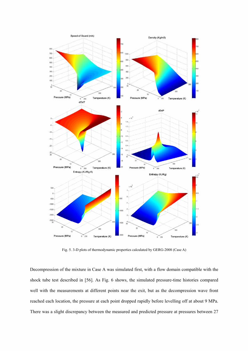
Fig. 5. 3-D plots of thermodynamic properties calculated by GERG-2008 (Case A)
Decompression of the mixture in Case A was simulated first, with a flow domain compatible with the
shock tube test described in [56]. As Fig. 6 shows, the simulated pressure-time histories compared
well with the measurements at different points near the exit, but as the decompression wave front
reached each location, the pressure at each point dropped rapidly before levelling off at about 9 MPa.
There was a slight discrepancy between the measured and predicted pressure at pressures between 27

and 26 MPa. Apart from that, the predicted change in pressure agreed satisfactorily with the
experimental results.
Fig. 6. Comparison between predicted and measured pressure-time traces (Case A).
Fig. 7 shows the transient behaviour of the fluid temperature at the four locations closest to the outlet
boundary (rupture disc). The variations in the speed of sound and the outflow velocity are shown in
Fig. 8 and Fig. 9 respectively. The forms of the pressure-time and temperature-time curves were
similar. The fluid temperature suddenly dropped from its initial value to 276 K. The temperature
remained steady at this value for several time steps, creating a temperature plateau, before continuing
to drop steadily.
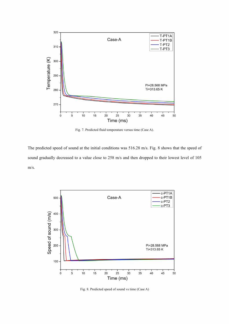
Fig. 7. Predicted fluid temperature versus time (Case A).
The predicted speed of sound at the initial conditions was 516.28 m/s. Fig. 8 shows that the speed of
sound gradually decreased to a value close to 258 m/s and then dropped to their lowest level of 105
m/s.
Fig. 8. Predicted speed of sound vs time (Case A)

Fig. 9. Predicted ‘outflow’ velocity versus time (Case A)
Before the rupture disk ruptured, the entire body of gas in the pipeline was at rest. In the simulation,
as the outlet boundary was subjected to ambient pressure at time t = 0+, an expansion
(decompression) wave was set off. As the wave propagated away from the opening, the exit velocity
was seen to increase. Like the other properties, the outlet velocity remained steady for a short time at
85 m/s before continuing to increase again.
Fig. 10 shows a comparison between the predicted and experimentally obtained decompression wave
speed. The predicted average decompression wave speed was obtained based on readings at the 6
pressure transducers listed in Table 3, whereas the local decompression wave speed was determined
using the predicted speed of sound and the ‘outflow’ velocity at 200 mm from the exit. Initially
(before the flow commenced), the speed of the decompression wave was equal to the predicted speed
of sound in the mixture because the ‘outflow’ speed was zero. The model predicted the initial
decompression wave speed well, differing by only 0.4% from the measured data. As the pressure
decreased the predicted average decompression wave speed agreed with the measured data, while the
local decompression wave speed varied slightly to the right of the experimental curve because the
‘local’ decompression wave speed was obtained using the formulation in Eq. (1), while the average
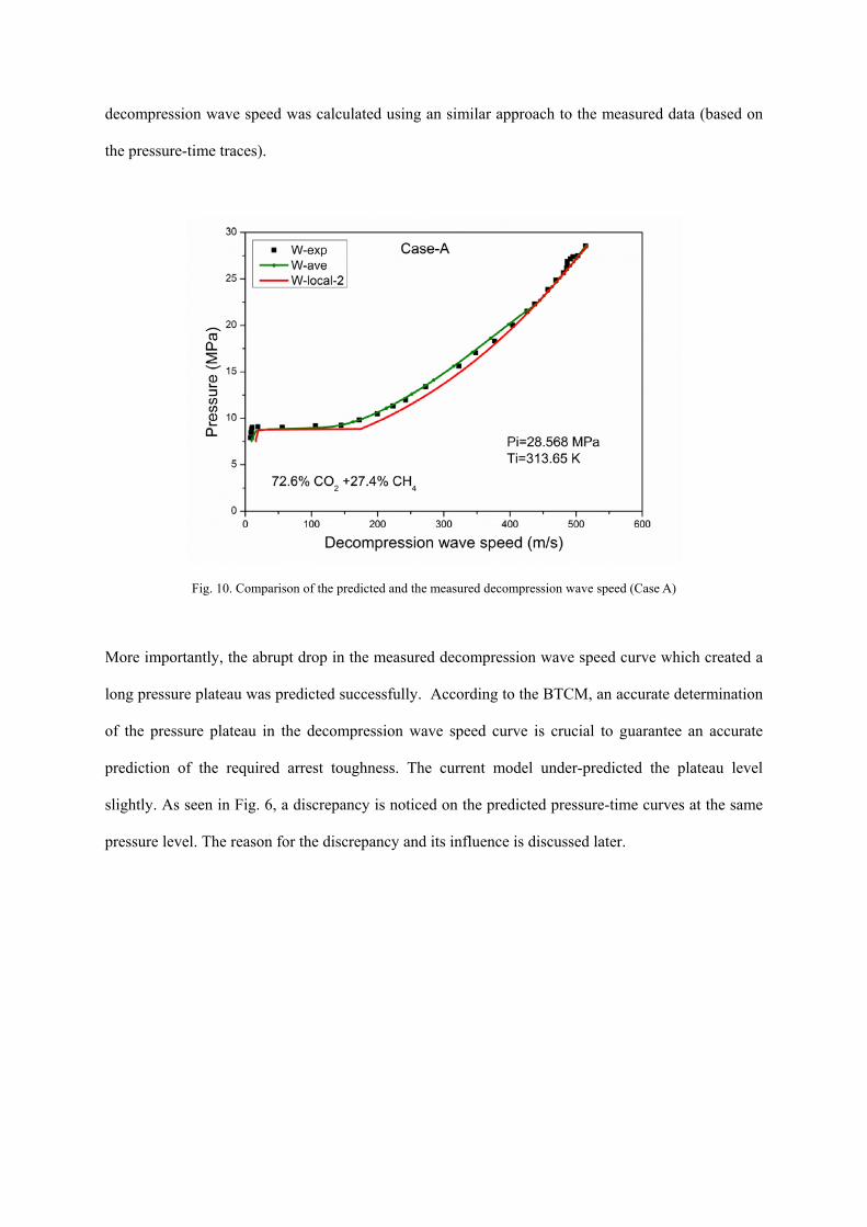
decompression wave speed was calculated using an similar approach to the measured data (based on
the pressure-time traces).
Fig. 10. Comparison of the predicted and the measured decompression wave speed (Case A)
More importantly, the abrupt drop in the measured decompression wave speed curve which created a
long pressure plateau was predicted successfully. According to the BTCM, an accurate determination
of the pressure plateau in the decompression wave speed curve is crucial to guarantee an accurate
prediction of the required arrest toughness. The current model under-predicted the plateau level
slightly. As seen in Fig. 6, a discrepancy is noticed on the predicted pressure-time curves at the same
pressure level. The reason for the discrepancy and its influence is discussed later.

Fig. 11. The pressure-temperature curve and the phase envelope (Case A)
The appearance of the plateau can be explained by superimposing the pressure-temperature gradient
on the phase envelope as depicted in Fig. 11. As the fluid crosses the phase boundary (at T=276 K, P
= 8.8 MPa), the decompression wave speed experiences a sharp drop which can be attributed to the
drop in the speed of sound, while simultaneously the monitored properties remained constant for
several time steps. Clearly, the trend that appeared in all properties stemmed from the discontinuity at
the phase boundary. Such outcomes demonstrate that the current CFD model can successfully deal
with the phase change predicted implicitly in the property tables.
The second simulation was for the mixture in Case B. The computational domain here was based on
the physical dimensions of the shock tube test described in [17]. Fig. 12 shows the CFD prediction of
pressure-time traces at 8 different pressure transducer locations along the pipe. A rapid drop in
pressure occurred as the decompression wavefront passed each location. The appearance of a plateau
at about 8 MPa can be ascribed to the phase change that occurred due to the decompression process.

Fig. 12. Predicted pressure-time traces (Case B)
Fig. 13 shows the drop in fluid temperature as a function of time at five different locations on the
tube. The temperature dropped rapidly from its initial value before flattening out for several time steps
at 277 K, creating a plateau in all curves. After this stage, the temperature steadily decreased to its
lowest value of 260 K which is predicted at the closest location towards the rupture disc. A
comparison with Fig. 14 shows that the plateaus occurred at the same pressure level as the point of
intersection of the pressure-temperature curve with the phase boundary.
Fig. 13. Predicted temperature-time traces (Case B)

Fig. 14. The decompression of pressure-temperature compared to phase envelope (Case B)
The speed of sound and the outflow velocity were both predicted in order to obtain the local
decompression wave speed. The predicted speed of sound versus time for five locations close to the
outlet is shown in Fig. 15, while the predicted outflow velocity is shown in Fig. 16. At the initial
pressure and temperature, the current model predicted the speed of sound as 522 m/s, while the
outflow velocity was 0m/s anywhere inside the tube (before flow commenced). A similar trend that
occurred in the outflow velocity of Case A occurred here where a kink appeared on all the curves due
to phase change. Referring back to the speed of sound curves, the phase change caused a decrease in
the speed of sound, and this overall drop in speed of sound due to discontinuity at the phase boundary
was ~350 m/s.
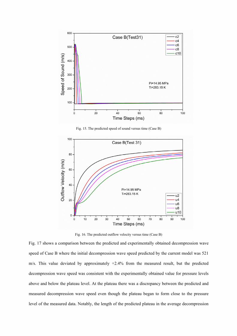
Fig. 15. The predicted speed of sound versus time (Case B)
Fig. 16. The predicted outflow velocity versus time (Case B)
Fig. 17 shows a comparison between the predicted and experimentally obtained decompression wave
speed of Case B where the initial decompression wave speed predicted by the current model was 521
m/s. This value deviated by approximately +2.4% from the measured result, but the predicted
decompression wave speed was consistent with the experimentally obtained value for pressure levels
above and below the plateau level. At the plateau there was a discrepancy between the predicted and
measured decompression wave speed even though the plateau began to form close to the pressure
level of the measured data. Notably, the length of the predicted plateau in the average decompression

wave speed curve was consistent with the measured data. Further discussion will be made hereafter.
Fig. 17. Comparison of the predicted decompression wave speed with the measured results (Case B)
5. Discussion
If the variation in the simulated pressure matches the experimental results (Fig. 6), the predicted
average value of the decompression wave speed W should agree with the measured curve (Fig. 10),
but as Fig. 10 shows, there was a slight discrepancy at the plateau between the predicted and
experimentally obtained decompression wave speed. This variation appeared at the same pressure
levels on the pressure-time curves, as Fig. 6 shows. There was major difference at the plateau level on
the decompression wave speed in the second case, as Fig. 17 shows. Such a variation may result from
uncertainties inherent in the numerical method and/or the way of implementing the GERG-2008 EOS,
although factors such as delayed nucleation and/or rapid phase change dynamics (not considered here)
can influence the results to various degrees. Another possible reason for this discrepancy was the
actual amount of impurities in the experimental tests which could be slightly different from the listed
composition.
The speed of sound in the current model can be tracked as a function of time so its relationship with
the decompression wave speed can be clearly understood. For instance, Fig. 17 shows that the ‘length’
of the pressure plateau (~348 m/s) was almost equal to the sharp drop in the speed of sound due to the
phase change, as seen in Fig. 15.
Fig. 10 and Fig.17 show long pressure plateaus that correspond to a significant drop in the
decompression wave speed. This would surely influence the ductile fracture propagation control, as
outlined in the BTCM. An example is shown in Fig. 18, where the BTCM was used to predict the
CVN value of pipe, grade 480 (X70). The diameter and wall thickness of the pipe was 609.6 mm and
19.1 mm respectively. Based on the predicted average decompression wave speed, the corresponding
CVN was ~105 J while the CVN value based on the experimentally determined decompression wave
speed was ~115 J [56]. The difference between prediction and measurement can be attributed to the
difference in the plateau level in the decompression wave speed, because the current CFD model
slightly under-predicted the pressure plateau level.
For modern higher grade steels, if the predicted CVN value is greater than ~95 J [57], then the CVN
value should be corrected using a certain correction factor to match the results of full-scale burst tests
[58, 59]. The Australian Standard (AS 2885.1), states that the predicted toughness should be
multiplied by a factor of at least 1.4. Fig. 18 shows the decompression wave speed and the fracture
propagation speed as functions of pressure. By applying the correction factor, the predicted CVN
becomes 147 J whereas the measured value was 161 J. Note that the accuracy of the plateau level in
the decompression wave speed was within ±0.1 MPa, the size of the pressure step used in the
calculation Wave.
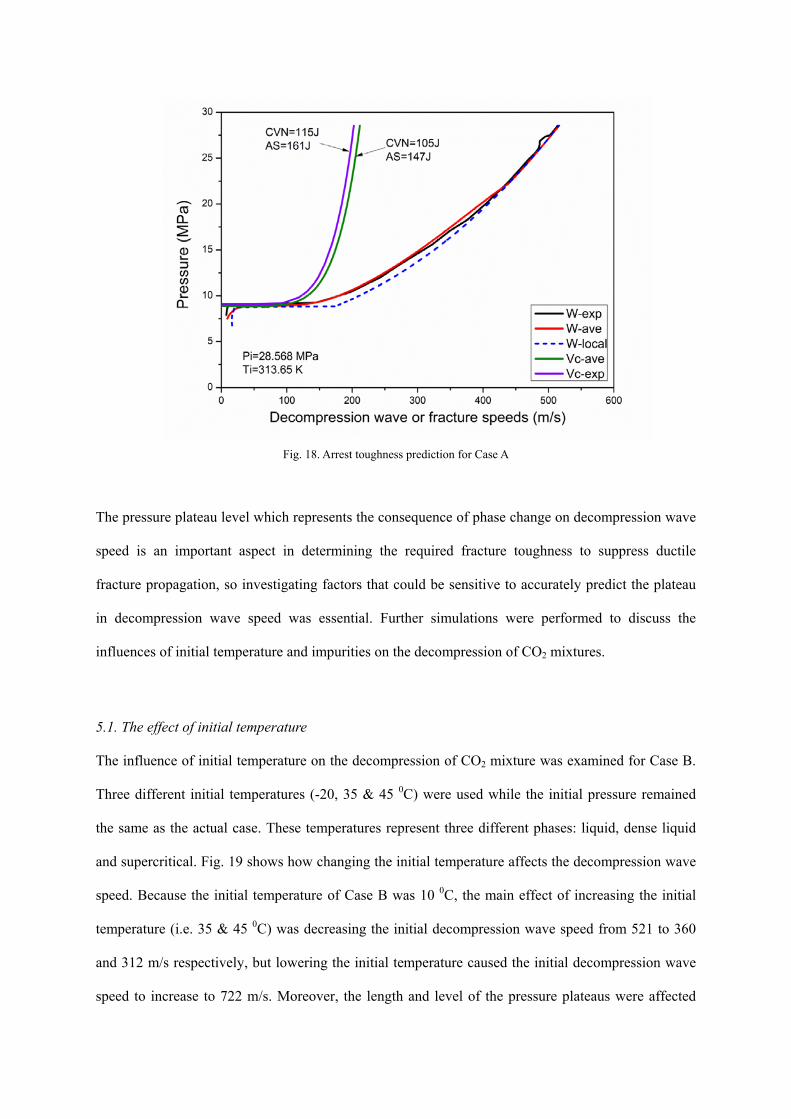
Fig. 18. Arrest toughness prediction for Case A
The pressure plateau level which represents the consequence of phase change on decompression wave
speed is an important aspect in determining the required fracture toughness to suppress ductile
fracture propagation, so investigating factors that could be sensitive to accurately predict the plateau
in decompression wave speed was essential. Further simulations were performed to discuss the
influences of initial temperature and impurities on the decompression of CO2 mixtures.
5.1. The effect of initial temperature
The influence of initial temperature on the decompression of CO2 mixture was examined for Case B.
Three different initial temperatures (-20, 35 & 45 0C) were used while the initial pressure remained
the same as the actual case. These temperatures represent three different phases: liquid, dense liquid
and supercritical. Fig. 19 shows how changing the initial temperature affects the decompression wave
speed. Because the initial temperature of Case B was 10 0C, the main effect of increasing the initial
temperature (i.e. 35 & 45 0C) was decreasing the initial decompression wave speed from 521 to 360
and 312 m/s respectively, but lowering the initial temperature caused the initial decompression wave
speed to increase to 722 m/s. Moreover, the length and level of the pressure plateaus were affected

due to changing the initial temperature; increasing the initial temperature decreased the length of the
plateau in the decompression wave speed, and vice versa. Those observations were consistent with the
predicted results of pure CO2 conducted by [60] and for mixtures e.g. [14, 56]. However, this effect
was different in terms of plateau levels for CO2 mixtures because it depended on the shape of the
bubble curve on phase envelope, which in turn depended on the amount and type of impurities in the
CO2 mixture.
Fig. 19. Initial temperature effect on decompression wave speed (Case A).
Increasing the initial temperature to 35 and 45 0C raised the level of plateaus by a value of 1 MPa
above the main test. Interestingly, as Fig. 19 shows, the apparent plateaus in these two cases occurred
at approximately the same level. This can be further explained by representing the pressure-
temperature profiles on the phase envelope of the mixture, as depicted in Fig. 20, but note that the
phase change occurred at approximately the same pressure level despite different intercept
temperatures with the phase boundary which were clearly due to the effect of impurities that rose up
the bubble curve on the phase envelope. Such a situation cannot occur for pure CO2.

Where the initial temperature was -20 0C, despite the initial decompression wave speed being much
higher than in the main test, the plateau level was predicted at a lower pressure level than the main
test by 0.5 MPa. Although this was consistent with the trend in the results of pure CO2 conducted by
[60], it cannot be taken as a role for CO2 mixtures because of the shape of the phase boundary. For
instance, if the initial temperature was less than (-20 0C), the intersection with the phase boundary
would take place at a higher pressure levels because the bubble curve increased again at temperature
level below that value. So the trend in the results of pure CO2 which states that as the initial
temperature decreases the plateau level in the decompression wave speed decreases cannot be applied
for CO2 mixtures.
Fig. 20. Intersection points with the phase envelope for different initial temperatures (Case B)
5.2. Influence of Impurities
The effects of several impurities (components other than CO2) on the decompression of CO2 pipelines
were examined. The impurities that were most likely to exist in carbon dioxide capture technologies
were used [61]. Table 5 lists the four binary CO2 mixtures studied, with the initial conditions.
Fig. 21 illustrates the effect of impurities on the phase envelope of CO2, and show that adding

impurities to pure CO2 shifts the critical point and the bubble curve in the phase envelope. Notably, an
addition 5% of hydrogen to the CO2 had more effect on the phase equilibrium than the other
impurities because it shifted the critical pressure to a value close to 10 MPa.
Table 3 The initial conditions of the predominantly CO2 mixtures.
Case no. Mixture components (mole %)
Pi (Mpa) Ti (K) CO2 H2 N2 O2 CO
Case1 95 5 0 0 0 15 283.15
Case2 95 0 5 0 0 15 283.15
Case3 95 0 0 5 0 15 283.15
Case4 95 0 0 0 5 15 283.15
Simulations of decompression with these binary mixtures were conducted using the same flow
domain as in Case A. Fig. 22 shows the influence on the decompression wave speed such that at the
same initial conditions and for a fixed fraction of CO2, each impurity resulted in a different initial
decompression wave speed and different pressure plateau level that was clearly related to the phase
envelope of the mixture. Adding 5% H2 to the CO2 resulted in the highest pressure plateau level (~ 9
MPa). Adding 5% N2 resulted in a pressure plateau of about 6 MPa. These changes in the
decompression wave speed could influence the fracture propagation/arrest requirements for CO2
pipelines.

Fig. 21. Phase envelope of CO2 mixtures calculated by GERG-2008 EOS.
Fig. 22. Impurities effect on CO2 decompression wave speed
6. Conclusion
Transporting CO2 mixtures by pipelines is a challenge. In order to improve our knowledge it is
important for the modelling tools to handle CCS CO2 mixtures efficiently. The feasibility of complex
and possibly large simulations of fluid-pipe interactions, hydraulic transients and dispersion will
otherwise be restricted. This paper has described a CFD model developed using ANSYS Fluent to
simulate the decompression behaviour of CO2 mixtures. For the first time ever, GERG-2008 EOS was
successfully implemented into ANSYS Fluent using UDFs based on an indirect use of the GERG-
2008 EOS library. This was done by using pre-compiled thermodynamic property tables (“lookup
tables”) linked to Fluent during simulation time. Several obstacles related to the EOS library were
avoided using this method.
The predicted results were validated against two separate ‘shock tube’ tests. The results mostly agreed
with the experimental results available. The following observations were made:
The CFD model successfully tracked the rapid drop in pressure and accounted for the phase
change during decompression.
The decompression wave speed curves in CO2 mixtures exhibited long pressure plateaus.
At the same initial pressure, increasing the initial operating temperature decreases the initial
decompression wave speed; and lowering the initial temperature increases the initial
decompression wave speed.
A drop in the initial temperature did not always result in a lower pressure plateau level for
CO2 mixtures.
The existence of hydrogen in CO2 stream had a maximum impact on decompression,
compared to the other impurities tested; CO, O2, and N2.
Overall, the current work shows that the CFD technique can be used to predict rapid and severe gas
decompression by solving the governing flow equations, in conjunction with the GERG-2008 EOS.
This is an effective tool for determining the decompression wave speeds for several CO2-based
mixtures and it is also applicable in two- or three-dimensional geometries so the effect of pipe
diameter, surface roughness and the shape of fracture outlet can be investigated. The implementation
of GERG-2008 allows modelling the real behaviour of CO2 mixture under failure events. This brought
about the possibility of using the CFD to investigate several areas related CCS (i.e. the dispersion of
CO2).
Future work will focus on developing a 3D decompression model so the effects of pipe opening and
the pressure drop behind the crack tip can be identified. A 3D coupled fracture-decompression model
is also a target to understand the interaction between the fracturing pipe and decompressing fluid.
7. Acknowledgement
This work was funded by the Energy Pipelines CRC, supported through the Australian Government’s
Cooperative Research Centre Program, and co-funded by the Department of Resources, Energy and
Tourism (DRET). The funding and in-kind support from the APIA RSC is gratefully acknowledged.
References
1. IE, 2011 Building Essential Infrastructure for Carbon Capture and Storage. Insight Economics
Pty Ltd (IE): Melbourne. p. 43. 2. Li, H. and J. Yan, 2009, Evaluating cubic equations of state for calculation of vapor–liquid
equilibrium of CO2 and CO2‐mixtures for CO2 capture and storage processes. Applied Energy. 86(6): p. 826‐836.
3. Metz, B., O. Davidson, H.d. Coninck, M. Loos, and L. Meyer, 2005 IPCC Special Report on Carbon Dioxide Capture and Storage. Intergovernmental Panel on Climate Change: New York. p. 443.
4. Zhang, Y., X. Ji, and X. Lu, 2014, Energy consumption analysis for CO2 separation from gas mixtures. Applied Energy. 130(0): p. 237‐243.
5. IEA, 2010 CO2 pipeline Infrastructure: An analysis of global challenges and opportunities. International Energy Agency Greenhouse Gas Programme. p. 1‐134.
6. DNV, 2010, Recommended Practice DNV‐RP‐J202 "Design and Operating of CO2 Pipelines". 7. Cosham, A. and R.J. Eiber, 2008a, Fracture propagation in CO2 pipelines. The Jornal of
Pipeline Engineering. 4: p. 281‐291. 8. Li, H. and J. Yan, 2009, Impacts of equations of state (EOS) and impurities on the volume
calculation of CO2 mixtures in the applications of CO2 capture and storage (CCS) processes. Applied Energy. 86(12): p. 2760‐2770.
9. Maxey, W.A., J.F. Kiefner, and R.J. Eiber,1976 Ductile fracture arrest in gas pipelines. Related Information: A. G. A. Cat. No. L32176. Medium: X; Size: Pages: 46.

10. Kiefner, J.F., W.A. Maxey, R.J. Eiber, and A.R. Duffy, 1973 Failure Stress Levels of Flaws in Pressurized Cylinders Progress in Flaw Growth and Fracture toughness Testing, ASTM STP 536, American Society for Testing and Materials. p. 461‐481.
11. Rothwell, A.B., 2000, Fracture propagation control for gas pipelines––past, present and future. In: Denys R, editor. Proceedings of the 3rd International Pipeline Technology Conference. 1: p. 387–405.
12. Eiber, R., T. Bubenik, and W. Maxey, 1993 GASDECOM, computer code for the calculation of gas decompression speed that is included in fracture control technology for natural gas pipelines. NG‐18 Report 208. American Gas Association Catalog.
13. Starling, K.E. and J.E. Powers, 1970, Enthalpy of Mixtures by Modified BWR Equation. Industrial & Engineering Chemistry Fundamentals. 9(4): p. 531‐537.
14. Cosham, A., R.J. Eiber, and E.B. Clark, 2010, GASDECOM: Carbon Dioxide and Other Components. ASME Conference Proceedings. 2: p. 777‐794.
15. Hopke, S.W. and C.J. Lin, 1974 Application of BWRS Equation to Natural Gas Systems, in 76'h National AIChE Meeting, American Institute of Chemical Engineers: Tulsa, Oklahoma, USA.
16. Phillips, A.G. and C.G. Robinson, 2002 Gas decompression behavior following the rupture of high pressure pipelines ‐ Phase 1, PRCI Contract PR‐273‐0135. Pipeline Research Council International, Inc. p. 1‐52.
17. Cosham, A., D.G. Jones, K. Armstrong, D. Allason, and J. Barnett. 2012a, The Decompression Behaviour oF Carbon Dioxide in The Densephase. in Proceedings of the 2012 9th International Pipeline Conference. Calgary, Alberta, Canada: ASME.
18. Lemmon, E.W., M.L. Huber, and M.O. McLinden, 2010 NIST Standard Reference Database 23: Reference Fluid Thermodynamic and Transport Properties‐REFPROP. National Institute of Standards and Technology: Gaithersburg.
19. Span, R. and W. Wagner, 1996, A New Equation of State for Carbon Dioxide Covering the Fluid Region from the Triple‐Point Temperature to 1100 K at Pressures up to 800 MPa. ISSN. 25(6): p. 1509‐1596.
20. Kunz, O., R. Klimeek, W. Wagner, and M. Jaeschke, 2007 The GERG‐2004 Wide‐Range Equation of State for Natural Gases and Other Mixtures‐GERG Technical Monograph 15. Groupe Européen de Recherches Gazières.
21. Picard, D.J. and P.R. Bishnoi, 1988, The Importance of Real‐Fluid Behavior and Nonisentropic Effects in Modeling Decompression Characteristics of Pipeline Fluids for Application in Ductile Fracture Propagation Analysis. THE CANADIAN JOURNAL OF CHEMICAL ENGINEERING. 66(1): p. 3‐12.
22. Picard, D.J. and P.R. Bishnoi, 1989, The Importance of Real‐Fluid Behavior in Predicting Release Rates Resulting From High‐Pressure Sour‐Gas Pipeline Ruptures. THE CANADIAN JOURNAL OF CHEMICAL ENGINEERING. 67(1): p. 3‐9.
23. Mahgerefteh, H., S. Brown, and G. Denton, 2012, Modelling the impact of stream impurities on ductile fractures in CO2 pipelines. Chemical Engineering Science. 74(0): p. 200‐210.
24. Mahgerefteh, H., S. Brown, and S. Martynov, 2012, A study of the effects of friction, heat transfer, and stream impurities on the decompression behavior in CO2 pipelines. Greenhouse Gases: Science and Technology. 2(5): p. 369‐379.
25. Jie, H.E., B.P. Xu, J.X. Wen, R. Cooper, and J. Barnett. 2012, Predicting The Decompression Characteristics of Carbon Dioxide Using Computational Fluid Dynamics. in Proceedings of the 2012 9th International Pipeline Conference. Calgary, Alberta, Canada ASME.
26. Lu, C., G. Michal, A. Elshahomi, A. Godbole, P. Venton, K.K. Botros, L. Fletcher, and B. Rothwell. 2012, Investigating The Effects of Pipe Wall Roughness and Pipe Diameter on The decompression Wave Speed in Natural Gas Pipelines. in 9th International Pipeline Conference 2012. Calgary, Alberta, Canada: ASME.
27. Botros, K.K., L. Carlson, and M. Reed, 2013a, Extension of the semi‐empirical correlation for the effects of pipe diameter and internal surface roughness on the decompression wave
speed to include High Heating Value Processed Gas mixtures. International Journal of Pressure Vessels and Piping. 107: p. 12‐17.
28. Botros, K.K., J. Geerligs, L. Fletcher, B. Rothwell, P. Venton, and L. Carlson, 2010d, Effects of Pipe Internal Surface Roughness on Decompression Wave Speed in Natural Gas Mixtures. ASME Conference Proceedings. 2010(44212): p. 907‐922.
29. Botros, K.K., B. Rothwell, L. Carlson, and P. Venton, 2012 Semi‐Empirical Correlation to Quantify the Effects of Pipe Diameter and Internal Surface Roughness on the Decompression Wave Speed in Natural Gas Mixtures in 9th International Pipeline Conference IPC2012. ASME: ,Calgary, Alberta, Canada
30. Chen, J.R., S.M. Richardson, and G. Saville, 1995, Modelling of two‐phase blowdown from pipelines—II. A simplified numerical method for multi‐component mixtures. Chemical Engineering Science. 50(13): p. 2173‐2187.
31. Bendiksen, K.H., D. Maines, R. Moe, and S. Nuland, 1991, The Dynamic Two‐Fluid Model OLGA: Theory and Application. SPE Production Engineering. 6(2): p. 171‐180.
32. Zucrow, M.J. and J.D. Hoffman,1976 Gas Dynamics. New York: John Wiley and Sons. 33. Mahgerefteh, H., A. Oke, and O. Atti, 2006, Modelling outflow following rupture in pipeline
networks. Chemical Engineering Science. 61(6): p. 1811‐1818. 34. Mahgerefteh, H., Saha, Pratik, Economou, and I. G., 1999, Fast numerical simulation for bore
rupture of pressurized pipelines. American Institute of Chemical Engineers. AIChE Journal. 45(6): p. 1191‐1191.
35. Brown, S.F., 2011 CFD Modelling of Outflow and Ductile Fracture Propagation in Pressurised Pipelines, in Department of Chemical Engineering. University College London: London. p. 227.
36. Peng, D.‐Y. and D.B. Robinson, 1976, A New Two‐Constant Equation of State. Industrial & Engineering Chemistry Fundamentals. 15(1): p. 59‐64.
37. Starling, K.E. and J.L. Savidge, 1994 Compressibility Factors of Natural Gas and Other Related Hydrocarbon Gases. American Gas Association, Transmission Measurement Committee Report No.8, and American Petroleum Institute, MPMS Chapter 14.2 Second Edition.
38. Picard, D.J. and P.R. Bishnoi, 1987, Calculation of the thermodynamic sound velocity in two‐phase multicomponent fluids. International Journal of Multiphase Flow. 13(3): p. 295‐308.
39. Li, H., J.P. Jakobsen, Ø. Wilhelmsen, and J. Yan, 2011, PVTxy properties of CO2 mixtures relevant for CO2 capture, transport and storage: Review of available experimental data and theoretical models. Applied Energy. 88(11): p. 3567‐3579.
40. Patel, N.C. and A.S. Teja, 1982, A new cubic equation of state for fluids and fluid mixtures. Chemical Engineering Science. 37(3): p. 463‐473.
41. Redlich, O. and J.N.S. Kwong, 1949, On the Thermodynamics of Solutions. V. An Equation of State. Fugacities of Gaseous Solutions. Chemical Reviews. 44(1): p. 233‐244.
42. Soave, G., 1972, Equilibrium constants from a modified Redlich‐Kwong equation of state. Chemical Engineering Science. 27(6): p. 1197‐1203.
43. Péneloux, A., E. Rauzy, and R. Fréze, 1982, A consistent correction for Redlich‐Kwong‐Soave volumes. Fluid Phase Equilibria. 8(1): p. 7‐23.
44. Hu, J., Z. Duan, C. Zhu, and I.‐M.C. c, 2006, PVTx properties of the CO2–H2O and CO2–H2O–NaCl systems below 647 K: Assessment of experimental data and thermodynamic models. Chemical Geology. 238: p. 249–267.
45. Yu, J.‐M., B.C.Y. Lu, and Y. Iwai, 1987, Simultaneous calculations of VLE and saturated liquid and vapor volumes by means of a 3P1T cubic EOS. Fluid Phase Equilibria. 37(0): p. 207‐222.
46. Ji, W.‐R. and D.A. Lempe, 1997, Density improvement of the SRK equation of state. Fluid Phase Equilibria. 130(1–2): p. 49‐63.
47. Liu, X., A. Godbole, C. Lu, G. Michal, and P. Venton, 2014, Source strength and dispersion of CO2 releases from high‐pressure pipelines: CFD model using real gas equation of state. Applied Energy. 126(0): p. 56‐68.

48. Botros, K.K., 2002, Performance of five equations of state for the prediction of vle and densities of natural gas mixtures in the dense phase region. Chemical Engineering Communications. 189(2): p. 151‐172.
49. Botros, K.K., 2010c, Measurements of Speed of Sound in Lean and Rich Natural Gas Mixtures at Pressures up to 37 MPa Using a Specialized Rupture Tube. International Journal of Thermophysics. 31(11): p. 2086‐2102.
50. Luo, X., M. Wang, E. Oko, and C. Okezue, 2014, Simulation‐based techno‐economic evaluation for optimal design of CO2 transport pipeline network. Applied Energy. 132(0): p. 610‐620.
51. Liou, M.S., 1993, A new flux splitting scheme. Journal of Computational Physics. 107(1): p. 23‐39.
52. Wagner, W., 2009 Description of the Software Package for the Calculation of Thermodynamic Properties from the GERG‐2004 XT08 Wide‐Range Equation of State for Natural Gases and Other Mixtures. RUHR‐UNIVERSITÄT BOCHUM. p. 76.
53. Wagner, W., 2009 Description of the Software Package for the Calculation of Thermodynamic Properties from the GERG‐2004 XT08 Wide‐Range Equation of State for Natural Gases and Other Mixtures. Ruhr‐Universitat Bochum. p. pp.76.
54. Andresen, T. and G. Skaugen. 2007, Lookup Tables Based on Gibb’s Free Energy for Quick and Accurate Calculation of Thermodynamic Properties for CO2. in 22nd International Congress of Refrigeration : Refrigeration creates the future. Beijing: International Institute of Refrigeration.
55. Mahgerefteh, H., O. Atti, and G. Denton, 2007, An Interpolation Technique for Rapid CFD Simulation of Turbulent Two‐Phase Flows. Process Safety and Environmental Protection. 85(1): p. 45‐50.
56. Botros, K.K., E.H. Jr, and P. Craidy, 2013b, Measuring decompression wave speed in CO2 mixtures by a shock tube. Pipelines International. (16).
57. Leis, B.N., X.‐K. Zhu, and T.P. Forte, 2009 New approach to assess running fracture arrest in pipelines, in Pipeline Technology Conference, 12‐14 October: Ostend, Belgium.
58. Hashemi, S.H., 2009, Correction factors for safe performance of API X65 pipeline steel. International Journal of Pressure Vessels and Piping. 86(8): p. 533‐540.
59. Wilkowski, G., D. Rudland, H. Xu, and N. Sanderson, 2006 Effect of Grade on Ductile Fracture Arrest Criteria for Gas Pipelines, in 2006 International Pipeline Conference. ASME: Calgary, Alberta, Canada, September 25–29, 2006.
60. Cosham, A., 2009, CO2: "It's a gas, Jim, but not as we Know it". Pipeline Technology Conference. p. 1‐16.
61. Seevam, P.N., J.M. Race, M.J. Downie, and P. Hopkins, 2008, Transporting the Next Generation of CO[sub 2] for Carbon, Capture and Storage: The Impact of Impurities on Supercritical CO2 Pipelines. ASME Conference Proceedings. 2008(48579): p. 39‐51.