deconvolving smooth residence time distributions from raw

��

�� !�

��

∀�� #�∃�#�∀��#�%�� &�∋(��#�)��∗+,−�.�/��0�∀(�� (�/��1��(��∀��/��2��3∋ ��0��4�0��0#�+,�∗−−.��)∀∀5�−,!�6,7��

�� 8� ��0�−,�−,7−�∗9∀:4.34�−�� 6��!��,,,−−�,

��

��;��

mailto:[email protected]

http://eprints.whiterose.ac.uk/

Deconvolving Smooth Residence Time Distributions from Raw1

Solute Transport Data2

F. Sonnenwald1, V. Stovin2, I. Guymer33

ABSTRACT4

A Residence Time Distribution (RTD) provides a complete model of longitudinal mixing5

effects that can be robustly derived from experimental solute transport data. Maximum6

entropy deconvolution has been shown to recover RTDs from pre-processed laboratory data.7

However, data pre-processing is time consuming and may introduce errors. Assuming data8

were recorded using sensors with a linear response, it should be possible to deconvolve raw9

data without pre-processing. This paper uses synthetically generated ‘raw’ data to demon-10

strate that the quality of the deconvolved RTD remains satisfactory when pre-processing11

steps involving data cropping or calibration are skipped. Provided noise levels are rela-12

tively low, filtering steps may also be omitted. However, a rough subtraction of background13

concentration is recommended as a minimal pre-processing step.14

Deconvolved RTDs often include small scale fluctuations that are inconsistent with a well-15

mixed fully turbulent system. These are believed to be associated with over-sampling and/or16

unsuitable interpolation functions used in the maximum entropy deconvolution process. This17

paper describes a new interpolation function—Linear interpolation with an Automatic Mov-18

ing Average (LAMA)—and demonstrates that, in combination with fewer sample points19

(e.g. 20), it enables smoother RTDs to be generated.20

The two improvements, to deconvolve raw data and to generate smoother RTDs, have21

1Research Associate, Department of Civil & Structural Engineering, The University of Sheffield, MappinSt., Sheffield S1 3JD, UK, e-mail: [email protected]

2Reader, Department of Civil & Structural Engineering, The University of Sheffield, Mappin St., SheffieldS1 3JD, UK, e-mail: [email protected]

3Professor, School of Engineering, University of Warwick, Coventry CV4 7AL, UK, e-mail:[email protected]

1 Sonnenwald, Feb. 2, 2014

been validated with experimental data. Raw solute transport traces collected from a river22

were deconvolved after background subtraction. The deconvolved RTDs compare favourably23

with those generated from the more traditional ADE and ADZ models, but provide more24

detail of mixing processes. A laboratory manhole solute transport data set was deconvolved25

with and without pre-processing using 40 sample points and linear interpolation. The raw26

data was also deconvolved using 20 sample points and LAMA interpolation. The two sets of27

RTDs deconvolved from the raw data show the same mixing trends as those deconvolved from28

pre-processed data. However, those deconvolved with LAMA interpolation and 20 sample29

points are significantly smoother.30

Keywords: Solutes, Dispersion, Mixing, Hydraulic models, Transfer functions, Residence31

time32

INTRODUCTION33

Solute transport traces, or temporal concentration profiles, recorded from complex flow34

systems (e.g. rivers or manholes) provide a description of the mixing processes occurring and35

are often analysed using parametrised models, e.g. fitting the Advection-Dispersion Equation36

(ADE) model or the Aggregated Dead Zone (ADZ) model (Rutherford 1994). Recent work37

has highlighted the use of Residence Time Distributions (RTDs) as a significantly more38

flexible approach to modelling solute transport. In this context, the RTD can exactly describe39

the mixing processes within a specific reach or structure (Guymer and Stovin 2011), and40

thereby provide additional insight into the mixing processes, e.g. Gooseff et al. (2011); Stovin41

et al. (2010a).42

The RTD is frequently used in chemical engineering to describe reaction mixers (Den-43

bigh and Turner 1984), and is analogous to the instantaneous unit hydrograph (Sherman44

1932). It is the system mixing response to a Dirac tracer pulse (instantaneous input) and45

is often referred to as a non-parametric model. Levenspiel (1972) describes the RTD as the46

distribution of lengths of time fluid takes to pass through a system. This definition of the47

RTD, used in this paper, assumes a linear time-invariant system, i.e. steady-state conditions,48


and therefore stationarity of the flow field. As such, the RTD can be expressed through the49

convolution integral in Eq. (1), where E(τ) is the RTD, u(t) is the upstream concentration50

profile, and y(t) is the downstream concentration profile.51

y(t) =∫

∞

−∞

E(τ)u(t− τ)dτ (1)

The Cumulative Residence Time Distribution (CRTD) is the integral of the RTD over52

time, notated as F (τ). In other hydrology contexts, the RTD as defined above is instead53

referred to as a Travel (or transit) Time Distribution, e.g. McGuire and McDonnell (2006).54

RTDs may also be used to explore catchment-scale processes that are not directly observable,55

e.g. groundwater transport (Rinaldo et al. 2011).56

Given regularly sampled paired time-series concentration data records for u(t) and y(t),57

solving for the RTD in the convolution integral is an ill-posed problem (Hansen 1998). The58

general solution is known as deconvolution, i.e. the reverse process of convolution. This is a59

common problem in many areas, where the identification of the underlying transfer function60

between two signals is desired. There are multiple approaches to deconvolution; see Mad-61

den et al. (1996) for a detailed review. To date, two main deconvolution approaches have62

been applied to solute transport data, geostatistical deconvolution (Fienen et al. 2006) and63

maximum entropy deconvolution (Stovin et al. 2010b). This paper presents two improve-64

ments to the maximum entropy deconvolution method to further enhance its suitability as65

a generic approach to the deconvolution of solute transport data (Sonnenwald 2014). These66

improvements are:67

1. The ability to deconvolve raw data, i.e. without the requirement of pre-processing.68

2. The ability to produce smoother RTDs, by changing the interpolation function and69

identifying appropriate numbers of sample points.70

After a brief introduction to maximum entropy deconvolution, the potential to deconvolve71

raw data is investigated. Subsequently, improvements to RTD smoothness are investigated.72


Finally, two validation cases are presented showing the benefits imparted by the proposed73

improvements.74

Maximum entropy deconvolution75

Maximum entropy deconvolution is a process by which non-linear optimisation is used76

to refine an estimate of the RTD based on upstream and downstream concentration profiles.77

Following Skilling and Bryan (1984), a Lagrangian function is created as a combination of78

an entropy function and a constraint function. By maximising the Lagrangian, a solution79

for the RTD is derived. This method is outlined below, and detailed in Stovin et al. (2010b),80

Sonnenwald et al. (2014), and Sonnenwald (2014).81

S(E) = −N∑

i=1

Ei∑N

j=1Ej

ln

Ei/∑N

j=1Ej

ri

(2)

C =

∑Ni=1(yi − yi)

2

∑Ni=1 y

2i

(3)

L(E, λ) = C + λS(E) (4)

To solve for the estimated RTD E, Eq. (2)–(4) are implemented in MATLAB (The82

MathWorks Inc. 2011; Schittkowski 1986) as a minimisation problem and then solved using83

the fmincon function with an active set algorithm. S is the objective function, an entropy84

function that evaluates shape and helps to encourage a smooth RTD. N is the number of85

points in the RTD. r is a next-neighbour moving average of E (Hattersley et al. 2008). C is a86

constraint function, which evaluates the goodness-of-fit of the predicted downstream profile87

y compared to the recorded profile using a variation of the R2t function (Young et al. 1980).88

L is the Lagrangian function. λ is the Lagrange multiplier, which is determined at each89

iteration by a gradient descent method as part of fmincon (The MathWorks Inc. 2011).90

The deconvolution problem is computationally simplified by solving only for a sub-91

sampled RTD in the entropy function, with linear interpolation used to estimate the re-92


mainder of the RTD between sample points. Sub-sampling is based on an initial guess of93

the RTD provided by inverse fast Fourier transform deconvolution, with more sample points94

being placed where the slope of the guessed RTD is greater. Sonnenwald et al. (2014) ad-95

ditionally recommended the following settings: 40 sample points, 350 iterations, and the R2t96

constraint function.97

Evaluation of RTD quality98

Deconvolved RTDs may be evaluated based on their predictive capability and on their99

smoothness. Predictive capability is evaluated by convolving the deconvolved RTD with the100

upstream profile used in the deconvolution process. The resulting predicted downstream101

profile is compared to the original downstream profile, i.e. the output is compared to the102

data used to generate it. For this comparison, Sonnenwald et al. (2014) suggest the use of103

the Nash-Sutcliffe Efficiency Index, R2, where a value of 1.0 indicates a perfect match and104

R2 ≤ 0 indicates no correlation (Nash and Sutcliffe 1970). Smoothness of an RTD may be105

evaluated by measuring its entropy using Eq. (2) (Sonnenwald et al. 2014). Values closer to106

zero indicate a smoother RTD.107

Where synthetic trace data has been generated from a known RTD, a third evaluation of108

a deconvolved RTD is possible: a direct comparison between the original and deconvolved109

RTDs. Sonnenwald (2014) suggests that the Average Percent Error (APE) metric (Kashe-110

fipour and Falconer 2000) is more suitable for comparing RTDs as it is significantly more111

sensitive to differences between profiles than R2. APE = 0 indicates a perfect correlation,112

while APE ≥ 100 indicates no correlation.113

THE DECONVOLUTION OF RAW DATA114

Introduction115

Raw data is the information collected directly from instrumentation and recorded as-is116

during experimental laboratory and field work, e.g. voltage readings from a fluorometer.117

In most cases raw data must be pre-processed before it can be analysed. Saiyudthong118


(2003) describes the pre-processing of laboratory solute transport data as a complex chain of119

operations consisting of calibration, subtraction of background concentration levels, filtering,120

and cropping the data record (reducing the length, or duration, of the record through data121

cut-off based on definitions of experiment start and end times).122

Researchers can spend significant amounts of time developing pre-processing steps that123

take into account their specific experimental setup. Guymer and O’Brien (2000) provide a124

long and detailed description of fluorometer calibration, smoothing, and temporal averag-125

ing. Kasban et al. (2010) clearly outline and document several pre-processing steps used126

when obtaining the RTD using radiotracers. Other work only summarises pre-processing,127

e.g. Guymer (1998), or effectively ignores it, e.g. Wallis and Manson (2005). While pre-128

processing is generally not the specific focus of the research, it can have an impact on the129

quality of the research findings. Joo et al. (2000) show how better pre-processing of train-130

ing data for an artificial neural network used in predicting coagulant dosing rate leads to a131

better learning rate, reduced error, and improved predictive capability. Poor pre-processing,132

e.g. excessive smoothing or cropping, may introduce errors or remove useful information133

about the system.134

Sonnenwald et al. (2014) demonstrated that maximum entropy deconvolution robustly135

identifies the RTD from pre-processed trace data collected from a variety of mixing sys-136

tems. Assuming a linear instrument response, deconvolution of raw data should prove to be137

equally robust, allowing for a reduction in the time spent on pre-processing and potentially138

reducing sources of errors. This section demonstrates the applicability of maximum entropy139

deconvolution to raw solute transport data through a sensitivity analysis and, as a result,140

recommends a minimum required level of pre-processing.141

Methodology: Raw solute transport data sensitivity analysis142

To investigate how input data impacts on the deconvolved RTD, a sensitivity analysis143

was carried out. A perfect synthetic trace, i.e. a pre-processed solute transport trace, was144

generated and then typical pre-processing steps were applied in reverse to create synthetic145


‘raw’ time-series. The raw data were then deconvolved.146

The recovered RTDs were scaled according to the mass-balance of the data they were147

derived from and then evaluated for predictive capability and quality using R2 and APE148

respectively. Although Sonnenwald et al. (2014) concluded that 40 sample points should149

generally be selected for deconvolution, subsequent work (described in the second part of150

this paper and in Sonnenwald (2014)) has shown that smoother RTDs can be described using151

only 20 sample points, with no loss of predictive capability. Therefore, 20 sample points were152

used here.153

Synthetic data154

To form a perfect synthetic base solute transport trace, an upstream concentration profile155

has been convolved with a known RTD to create a downstream profile. This trace, Figure 1a,156

is analogous to pre-processed data. The upstream profile was a Gaussian distribution with157

µ = 24.4 s, σ = 5.5 s, and dt = 0.15 s. An RTD was synthesised as a Guassian distribution158

with µ = 13.7 s, σ = 3.1 s,∫

∞

−∞E(t)dt = 1. The downstream profile is created by convolution159

using Eq. (1). Concentration levels below 10−4 were treated as below the limit of detection160

and set to 0. The synthetic trace is representative of data recorded from an experimental161

pipe configuration with an 88 mm diameter, 5 l/s flow, and a distance between instruments162

of 2.7 m (Guymer and O’Brien 2000).163

Pre-processing of raw solute transport traces generally consists of four steps: apply a164

calibration function; determine and subtract background concentration levels; filter noise;165

and determine the start and end of the signal data (i.e. experimental event), then crop166

data points before and after. The process of reversing these steps to create synthetic raw167

data is outlined below. Figure 1b shows an example synthetic raw trace after reversed168

pre-processing.169

Data extension170

Laboratory data is often recorded for a longer period than necessary to ensure that the171

experiment is fully captured. Here, the trace is synthetic and therefore complete. To simulate172


raw data, extra data points have been added to the start and end of the base trace. Data173

extension has been added as 0%, 10%, and 20% of trace length before and after the trace.174

Zeros were used in order to retain mass-balance. Figure 1b has a 10% extension.175

Addition of noise176

Recorded data is subject to random variation, i.e. noise, either from within the system177

or due to the instrumentation. The synthetic base trace has no noise, so to simulate realistic178

raw data, noise has been added according to a truncated normal distribution. The maximum179

noise level k is defined in terms of the peak upstream concentration, equal to 0%, 5%, 10%,180

or 20%. Noise is assumed to be normally distributed with µ = 0 and σ = k/3 between the181

limits of [−k, k]. 20% noise is representative of a maximum of 1 V of noise for a typical 5 V182

sensor and can be considered a conservatively high value. Figure 1b has 10% noise.183

Addition of background184

Background concentration refers to a constant or near-constant concentration level mea-185

sured independently of any experimental event. It is often present in laboratory setups,186

particularly in those utilising recirculating systems. Subtraction of background is usually187

carried out to leave only the change in concentration caused by the experiment. This can be188

done using an assumed mean value or linear function derived from the recorded concentration189

levels.190

To simulate raw data, a background concentration has been added to the base trace,191

either as a constant value or varying linearly with time (sloped background). Constant192

background takes the form of a mean background concentration level, defined as a fraction193

of peak upstream concentration. Values of 0%, 10%, and 20% have been used. Background194

slope has been applied on top of each mean background level as an additional -2.5% increasing195

to 2.5% of peak upstream concentration for positive slope or 2.5% decreasing to -2.5% for196

negative slope. Figure 1b has a 10% mean background with an increasing slope.197


Uncalibration198

Calibrating raw data for linear sensors consists of multiplication by a known factor to199

relate sensor reading to concentration level. To simulate raw data, multiplication by an200

‘uncalibration’ factor has been applied to take the base trace out of mass-balance. Factors201

have been chosen independently for the upstream and downstream profiles so that the peak202

values are the combinations of 2, 3, 4 or 5 V (16 total). In Figure 1b, both profiles have203

been uncalibrated to 3 V.204

Results: Impact of pre-processing on deconvolution205

The combinations of data extension, noise, background (sloped and constant), and un-206

calibration resulted in 1,728 synthetic raw traces being deconvolved.207

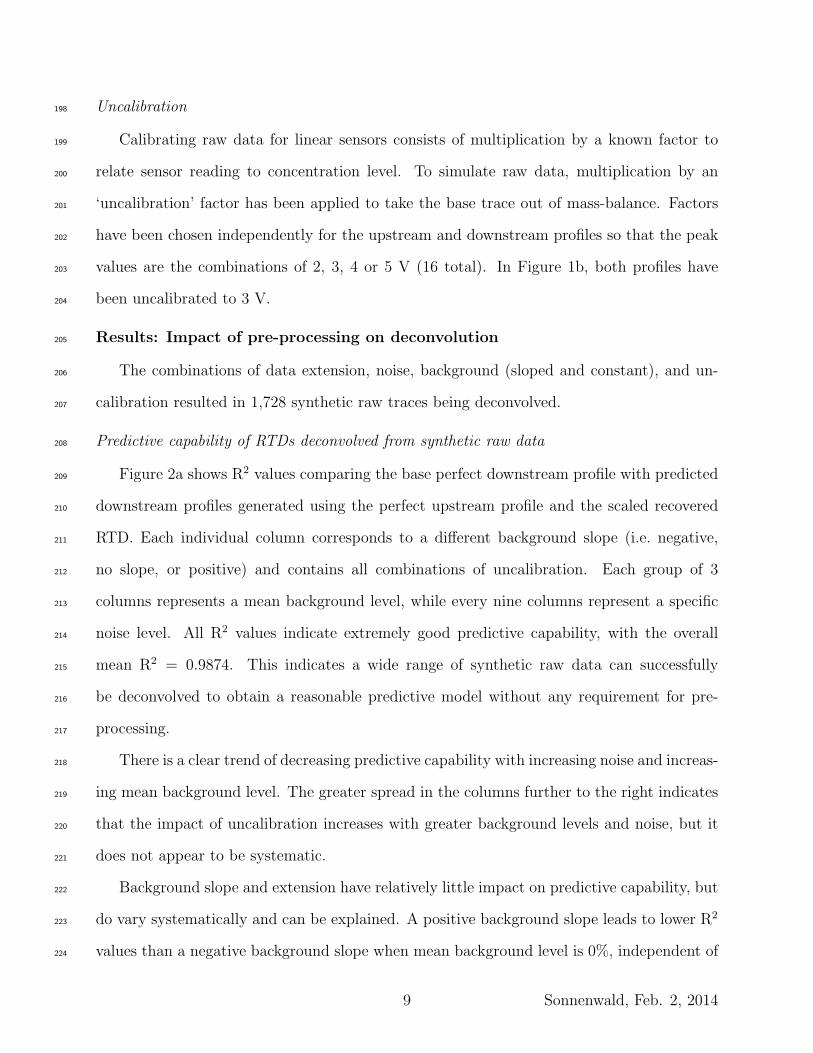
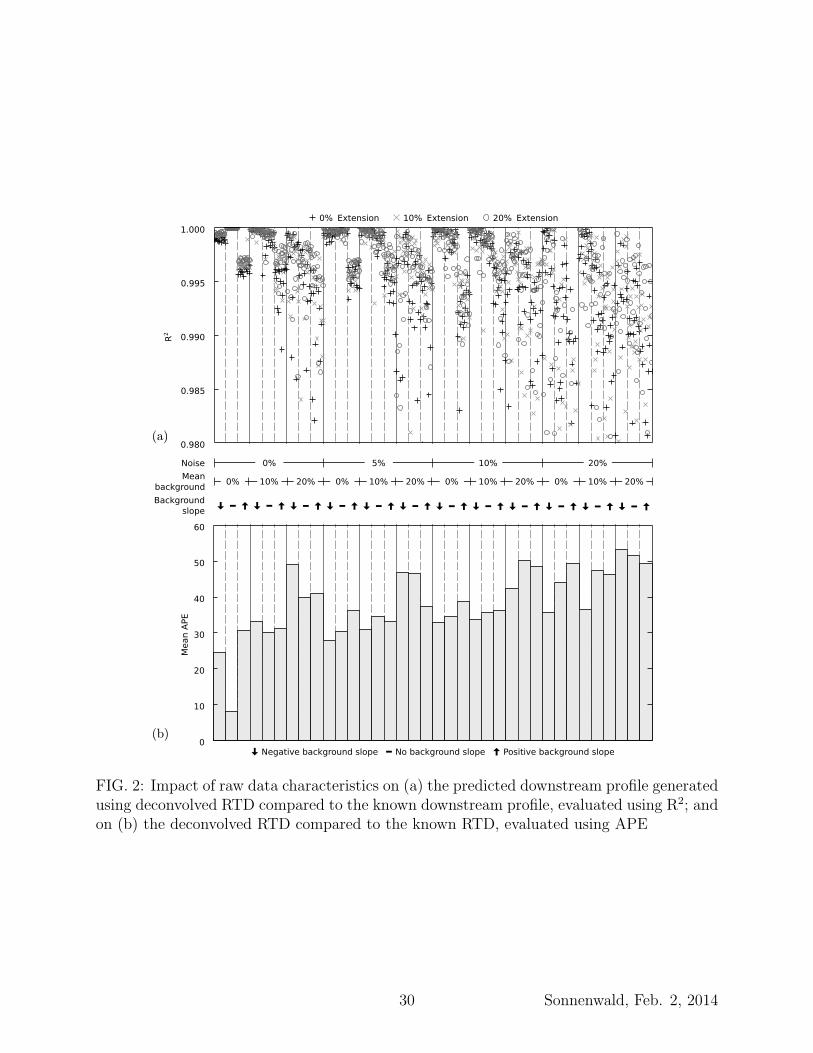
Predictive capability of RTDs deconvolved from synthetic raw data208

Figure 2a shows R2 values comparing the base perfect downstream profile with predicted209

downstream profiles generated using the perfect upstream profile and the scaled recovered210

RTD. Each individual column corresponds to a different background slope (i.e. negative,211

no slope, or positive) and contains all combinations of uncalibration. Each group of 3212

columns represents a mean background level, while every nine columns represent a specific213

noise level. All R2 values indicate extremely good predictive capability, with the overall214

mean R2 = 0.9874. This indicates a wide range of synthetic raw data can successfully215

be deconvolved to obtain a reasonable predictive model without any requirement for pre-216

processing.217

There is a clear trend of decreasing predictive capability with increasing noise and increas-218

ing mean background level. The greater spread in the columns further to the right indicates219

that the impact of uncalibration increases with greater background levels and noise, but it220

does not appear to be systematic.221

Background slope and extension have relatively little impact on predictive capability, but222

do vary systematically and can be explained. A positive background slope leads to lower R2223

values than a negative background slope when mean background level is 0%, independent of224


uncalibration. The negative portion of the downstream profile with a negative background225

slope cannot be matched in the deconvolution process, while the greater positive portion due226

to a positive background slope can be. RTDs deconvolved from the latter will more greatly227

over predict mass-balance than the former will under predict it. The greater over-prediction228

results in poorer R2 values.229

The increase of R2 with extension at no background and no noise may be explained by230

the wider spacing of sample points that results from the same 20 points being distributed231

over a longer profile. This reduces the relative potential for noise, leading to an improvement232

in RTD quality with extension. When there is non-zero background, there is a consistent233

period of time at the start of the profile when the downstream prediction does not match the234

recorded synthetic raw data. This period is fixed in length regardless of total duration and235

therefore, as extension increases, represents a proportionately smaller period of time. The236

period of poor fit therefore has less negative influence on the R2 value at greater extension,237

increasing R2 values overall.238

Quality of RTDs deconvolved from synthetic raw data239

Mean APE values for the comparison between the known and deconvolved RTDs are240

shown Figure 2b. The effects of extension and uncalibration have been combined as they have241

no systematic impact on predictive R2 value. The APE results show less variation than the242

predictive capability results, but can still be grouped similarly. This lower variation suggests243

the deconvolved RTDs have similar shapes despite the variation in input data quality. The244

lowest observed mean APE value is 8.21, indicating that the deconvolved RTD will always245

vary from the actual RTD. Background concentration appears to have a greater impact246

on RTD quality than noise, as the increase in APE observed when the background level247

increases from 10% to 20% is generally greater than when the noise level increases by the248

same amount. APE value generally increases less between 0% and 10% for both noise and249

background.250


Visual inspection of RTDs deconvolved from synthetic raw data251

Figure 3 shows representative deconvolved cumulative residence time distributions (CRTDs)252

for three cases. The first case has 5% noise and no background, the second case has 10%253

noise and 10% mean background (no slope), and the third case has 20% noise and 20% mean254

background (no slope). The third case CRTD includes values greater than 1, which in this255

case indicates a failure of the deconvolution method to cope with raw data that has high256

background concentration levels and high noise. Overall, the figure shows a reduction in257

CRTD quality (i.e. increasing APE) with increased noise and background. This confirms the258

results shown in Figure 2, and together they suggest 10% noise and 10% background levels259

as limits for deconvolved RTDs. The differences between 0% and 10% noise and background260

are much smaller than those between 10% and 20%. The 10% limit corresponds to approx-261

imate cut-offs of R2 = 0.995 and APE = 35 for this data set. Lower noise and background262

levels should be preferred to keep RTD quality high.263

Discussion: Recommendations for deconvolving raw data264

When deconvolving the synthetic raw data, predictive capability of the deconvolved RTD265

is generally good. Of the four pre-processing steps examined (data extension, noise, back-266

ground, and uncalibration), extension and uncalibration have been shown to have no sys-267

tematic impact on the deconvolved RTD, suggesting no pre-processing is necessary for these.268

However, increased noise and background concentration level both degrade predictive capa-269

bility and RTD quality in a similar fashion. As a result, 10% noise and 10% background270

have been suggested as input data quality limits for successfully deconvolving an RTD.271

These values are applicable to most types of input data since, as the RTD is non-parametric,272

the deconvolution process is independent of system scales and instead dependent on data273

characteristics.274

Background concentration is a common occurrence. It has a high impact on both pre-275

dictive capability and RTD quality, and is therefore important to address. Background con-276

centration should be subtracted as part of minimal pre-processing. This subtraction should277


take into account background slope, as increasing background concentration levels with time278

particularly influence the deconvolved RTD. However, it need not be overly precise, as at279

very low background levels noise will have a greater impact on the deconvolved RTD.280

Pre-processing for noise is unnecessary provided background subtraction has taken place.281

At 10% noise with no background, the RTD retains excellent predictive capability and satis-282

factory RTD shape. In the event of significantly greater noise levels, some filtering should be283

applied. Additional steps of down-sampling or cropping may be advisable for computational284

reasons when time-series are of significant length. However, in most cases no significant285

pre-processing should be required.286

Assuming that minimal pre-processing (in the form of subtracting background concen-287

tration level, taking into account background slope) is applied, this investigation has demon-288

strated that raw data can be successfully deconvolved.289

ENHANCED RTD SMOOTHNESS290

Introduction291

To date, RTDs derived with maximum entropy deconvolution have typically been pre-292

sented in their cumulative form as CRTDs. While this aids interpretation of the underlying293

mixing processes, the CRTD does not necessarily reveal small fluctuations in the RTD,294

e.g. those highlighted in Figure 4. These fluctuations numerically cancel out during convo-295

lution and so do not impact on the predictive capability of the RTD, but may potentially296

affect interpretation of the bulk mixing processes.297

The presence of fluctuations in deconvolved RTDs highlights a potential issue with the use298

of maximum entropy deconvolution, namely that a deconvolved RTD might not accurately299

represent some system characteristics. Considering that the cumulative effect of turbulence300

in most systems acts to smooth out fluctuations, if the deconvolution process were modified301

to minimise fluctuations, the quality of the resulting hydrodynamic interpretation should302

improve. A smoother RTD would aid interpretation as a more convincing representation of303

mixing processes.304


Fluctuations in deconvolved RTDs can in some cases be attributed to over-sampling305

of the sub-sample points used in the deconvolution process. Over-sampling occurs when306

too many sample points have been specified so that some points end up tightly clustered,307

which tends to result in significant fluctuation between adjacent sample point values. This308

section proposes an enhancement to maximum entropy deconvolution in the form of a new309

interpolation function to smooth the RTD and a re-evaluation of the number of sample310

points to reduce over-sampling, both of which should reduce fluctuations. Two alternative311

interpolation functions are proposed and a sensitivity analysis is carried out.312

Interpolation313

Interpolation is used by the maximum entropy deconvolution process to generate E, the314

estimated RTD. This is a critical part of the goodness-of-fit comparisons that are performed315

multiple times during each iteration. The interpolation function therefore plays an important316

role in influencing the deconvolved RTD.317

Linear interpolation (currently used), is the simplest type of interpolation. A straight318

line is drawn between the two closest sample points, and the interpolated data points are319

evaluated to be on that line. This has the benefit of being conceptually simple and easily320

executed. There are however, several more complex interpolation functions including Inverse321

Distance Weighting (IDW) and the Kriging Estimation Method (KEM), which are commonly322

used functions in GIS applications (Zimmerman et al. 1999). In IDW the point being inter-323

polated is defined to be more closely related to nearby points and less so to further points.324

In the KEM, the point being interpolated is derived as the result of a statistical model that325

estimates the relative importance of nearby points.326

In cubic interpolation (Fritsch and Carlson 1980), the sample points are used to estimate327

the derivatives of a cubic function that passes between them. The derivatives are then used328

to estimate the values at points being interpolated. Splines can also be used for interpolation.329

They are considered a subset of polynomial interpolation that are specified to have continuous330

n− 1 derivatives (de Boor 1978). A cubic spline has continuous first and second derivatives331


with the result that there are fewer possibilities for the interpolated line than using cubic332

interpolation.333

While any of the above interpolation functions could be used in the deconvolution pro-334

cess to smooth the RTD, a more pragmatic approach to smoothing is to apply a moving335

average after linear interpolation, i.e. linear interpolation with an automatic moving average336

(LAMA), outlined below. Initial investigation (Sonnenwald 2014) has shown this, and cubic337

interpolation, to be the most promising means of smoothing in this context and they are338

investigated further below.339

Methodology: RTD smoothness improvement sensitivity analysis340

A sensitivity analysis for evaluating improvements to RTD smoothness as a result of341

changing interpolation function and number of sample points has been carried out. Linear342

interpolation, cubic interpolation, and LAMA interpolation have been used to deconvolve343

three different solute transport traces. They have been deconvolved at between 15 and344

45 samples, as Sonnenwald et al. (2014) indicated that this range produced the smoothest345

results.346

The three solute transport traces correspond to: a solute transport trace collected from347

an 800 mm diameter surcharged manhole with flow at 1 l/s and surcharge at 268 mm348

(Guymer et al. 2005); a 24 mm pipe trace with transitional turbulent flow at 0.221 l/s (Hart349

et al. 2013); and a completely synthetic Gaussian trace. The latter was created specifically350

to demonstrate the effects of over-sampling. Assuming dt = 1 s, the upstream profile has351

µ = 25 s, σ = 5 s. The RTD has µ = 50 s, σ = 16.67 s. The area under both curves was352

normalised to 1 and the downstream profile created using Eq. (1).353

Implementing LAMA, linear interpolation with an automatic moving average354

The MATLAB interp1 function (The MathWorks Inc. 2011) has been used for cubic355

interpolation. However, as there is no convenient moving average function. Eq. (5), describ-356

ing a moving average, has been implemented. EMA(x) is the RTD with a moving average357

applied, 2α is the length of the moving average window size, and τ is an integration variable.358


In other words, the value EMA(x) is the mean of values of E from E(x− α) to E(x+ α).359

EMA(x) =∫ x+α

x−α

E(τ)

2αdτ (5)

In terms of the deconvolved RTD, a moving average can be considered a low-pass filter360

and the window size 2α a frequency cut-off. When applied to an RTD, high-frequency361

fluctuations shorter than the window size are removed, while the lower frequency mixing362

response is retained. Therefore, choice of window size is important. If 2α is too long,363

characteristics of the RTD (e.g. the peak associated with short-circuiting) may be overly364

attenuated. Conversely, a window size that is too short will not reduce fluctuations in the365

RTD.366

A method of directly estimating a suitable window size from an RTD has been developed367

so that the moving average filters only the higher frequency fluctuations. This is shown in368

Eq. (6), where tp is the time of the peak of the RTD, and tβ is the time at which the CRTD369

is equal to a fraction β of the CRTD at the peak of the RTD, i.e. tβ = βF (tp). As a result370

of the parameters used in Eq. (6), only the rising limb of the RTD affects the window size371

estimate. This reduces the risk of an asymmetric distribution (e.g. a non-Gaussian tail)372

skewing the window size estimate.373

2α = tp − tβ (6)

An initial evaluation of different values of β was conducted by deconvolving a collection374

of solute transport data for values of β = {0.05, 0.10, 0.15, 0.20}. Table 1 reports average R2375

depending on β. While in many cases there was no difference in performance, for some cases376

there is a drop in predictive capability when β = 0.05. This indicates that there is a penalty377

to predictive capability for using a low cut-off value (i.e. a longer window). All values of378

β had entropy values with the same order of magnitude and as such a value of 0.10 for β379

is a reasonable balance between smoothness and predictive performance under a variety of380


conditions.381

Within the deconvolution process, a new estimate of window size is made every time382

LAMA interpolation is applied. However, as finding the RTD is an optimisation process383

there are cases where an impossibly large window size can be estimated, which would then384

cause deconvolution to fail. For these scenarios, a maximum window size estimate (2αmax)385

has been specified. If 2α > 2αmax, 2α = 2αmax. 2αmax has been defined as twice the mean386

gap in sample point spacing around the peak of the guessed RTD used to sub-sample the387

RTD.388

Results: Impact of interpolation function and number of sample points on RTD389

smoothness390

To investigate the impact of interpolation function and number of sample points on RTD391

smoothness, 279 deconvolutions were carried out—the combination of 3 traces, 3 interpola-392

tion functions, and 31 different numbers of sample points. The mean R2 value overall was393

0.9992 with a minimum value of 0.9816 and maximum value of 1.0000, showing that all394

deconvolved RTDs form excellent predictive models. Figure 5 presents the predictive R2 and395

entropy values, the latter on a log scale, for each combination of interpolation function and396

number of sample points.397

The distribution of R2 values shows an increasing trend in predictive capability with398

more sample points. The relatively limited spread of R2 values at a given number of sample399

points shows that in most cases interpolation function has a lower impact than number of400

sample points on predictive capability. The systematic variation in R2 for the Synthetic401

data is caused by linear and cubic interpolation treating sample point values as observations402

through which the RTD must pass, while LAMA smooths these out. Overall there is no clear403

relationship between interpolation function and R2 value, which suggests that the choice of404

interpolation function should primarily be guided by entropy.405

Entropy values show increasing smoothness (i.e. values closer to zero) with fewer sample406

points. This is expected given the results of Sonnenwald et al. (2014) and confirms the407


impact that number of sample points can have on RTD quality. Independent of the number408

of sample points, the interpolation function also significantly impacts on entropy. LAMA409

interpolation performs best, with entropy values significantly and consistently closer to zero.410

Cubic and linear interpolation both show greater entropy, indicating they are less smooth.411

This suggests LAMA interpolation as the best choice for a smooth RTD.412

Visual inspection of smoothed RTDs413

Higher R2 values and entropy values closer to zero are to be preferred as being repre-414

sentative of smoother, higher quality RTDs. Number of sample points should be chosen415

(in combination with interpolation function) to provide a balance of predictive capability416

and smoothness. In this instance, with fewer than 20 sample points there is no appreciable417

improvement in entropy when using LAMA, and as a result there is no reason to reduce R2418

further by using fewer sample points.419

Figure 6 shows RTDs deconvolved with 20 sample points to be visibly smoother than420

the original 40 sample points. The figure also shows RTDs to be smoothest when using421

LAMA interpolation, with linear interpolation next smoothest and cubic interpolation least422

smooth. RTD shape is consistent, independent of the interpolation function and the number423

of sample points.424

Almost all of the 40 sample point RTDs show signs of over-sampling, with variation425

around the 20 sample point deconvolved RTDs. In the case of the synthetic trace, over-426

sampling is also visible at 20 sample points using linear and cubic interpolation, but not in427

the RTD deconvolved with LAMA interpolation. The LAMA interpolated RTD has an APE428

value of 1.08 indicating it is very close to the original RTD used to generate the synthetic429

pipe trace. In comparison, the cubic and linear interpolated RTDs have APE values of 10.26430

and 6.24 respectively, despite similar predictive capability.431

There is the potential that reduced numbers of sample points and LAMA interpolation432

may constrain the RTD, affecting hydraulic interpretation. However, there is no direct433

indicator of what RTD provides the “correct” hydraulic interpretation without additional434


observations. Ideally multiple dye injections should be recorded and deconvolved at both435

higher and lower numbers of sample points to reveal key system characteristics.436

Discussion: Recommendations for improving RTD smoothness437

Deconvolved RTDs generated using all combinations of interpolation function and num-438

ber of sample points result in RTDs with good predictive capability. R2 decreases in an439

approximately linear trend with decreasing number of sample points, although the relative440

differences in R2 are quite small. Entropy values of the LAMA interpolation function are441

consistently closer to zero, reflecting smoother RTDs than either linear or cubic interpola-442

tion. Visual inspection of the deconvolved RTDs shows that RTD shape remains consistent443

across interpolation function and number of sample points.444

The increased smoothness of the deconvolved RTDs is more consistent with expected445

system dynamics, and the removal of over-sampling effects is desirable for similar reasons.446

As the effects of turbulent mixing occur more rapidly than the system time-scale in most447

cases, the system is expected to be well mixed and therefore have a smooth RTD. Additionally448

the convolution process acts to average out rapidly changing fluctuations, and therefore they449

cannot be inferred from the deconvolution process. The result of a smoother RTD is one that450

more accurately reflects system hydrodynamics. Smoother RTDs are also easier to interpret451

and cross-compare.452

RTD smoothness did not increase at fewer than 20 sample points, while R2 value in some453

cases dropped. Therefore, 20 sample points is recommended as a reasonable compromise454

between predictive capability and entropy performance for obtaining a smooth RTD. More455

sample points may be necessary when the system the RTD is describing is more complex456

(e.g. multiple peaks). LAMA interpolation clearly results in the smoothest RTDs for each457

solute transport trace deconvolved. The synthetic data particularly demonstrates how the458

impact of over-sampling can be reduced using LAMA interpolation. Fewer sample points459

and LAMA interpolation have both clearly been shown to improve RTD smoothness and460

can therefore be recommended.461


VALIDATION462

Two validation cases have been examined. First, river data has been deconvolved with463

the proposed improvements. Secondly, the proposed improvements have been applied cumu-464

latively to an experimental manhole data set.465

Deconvolution of river solute transport data466

The UK Environment Agency has compiled a national database of river solute transport467

data, including solute traces (Guymer 2002). The traces recorded in the database were done468

so under varying conditions, e.g. different equipment, background concentration, etc. It469

presents a unique pre-processing challenge as for most types of analysis, data from each470

source must be treated differently. Trace data from the national database, recorded from471

the River Swale (NE17) at approximately an 18 m3/s flow rate, have been deconvolved.472

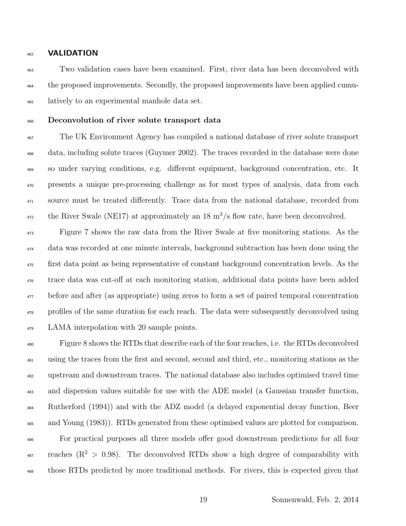
Figure 7 shows the raw data from the River Swale at five monitoring stations. As the473

data was recorded at one minute intervals, background subtraction has been done using the474

first data point as being representative of constant background concentration levels. As the475

trace data was cut-off at each monitoring station, additional data points have been added476

before and after (as appropriate) using zeros to form a set of paired temporal concentration477

profiles of the same duration for each reach. The data were subsequently deconvolved using478

LAMA interpolation with 20 sample points.479

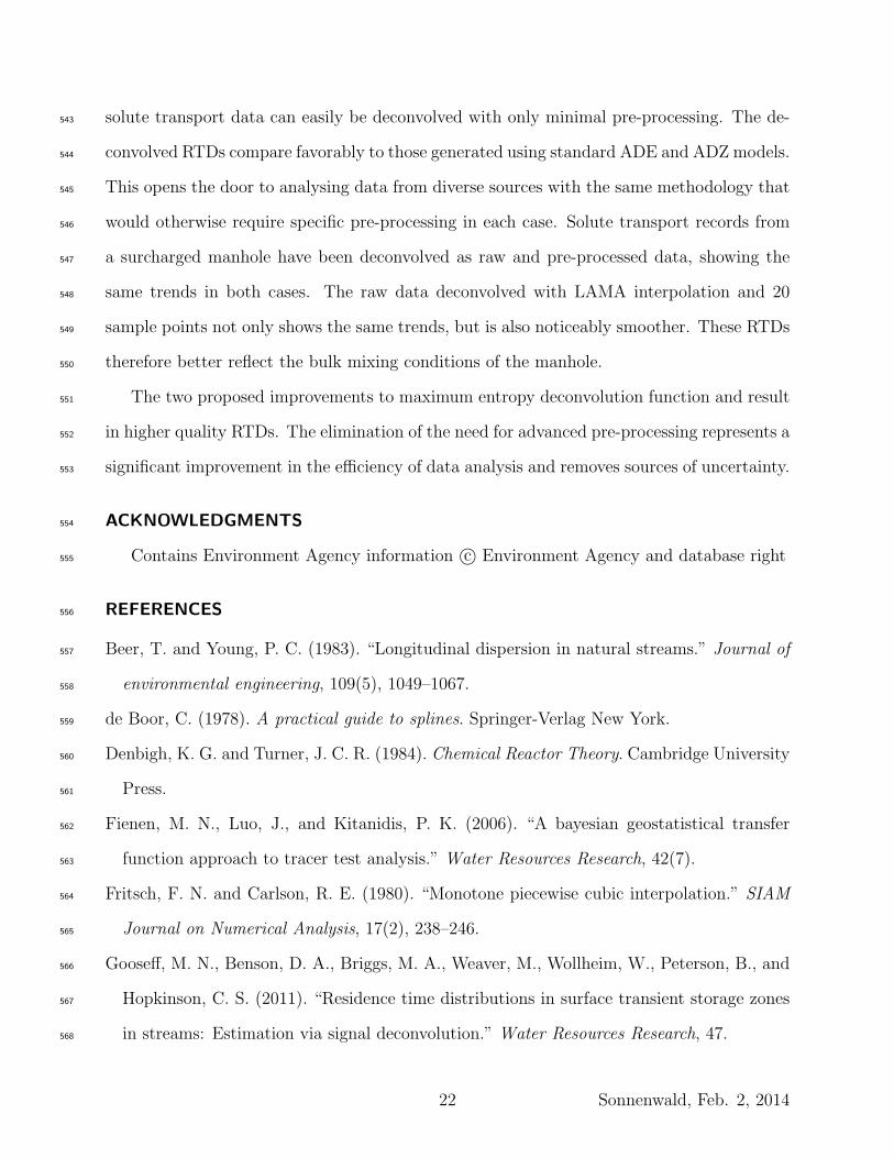
Figure 8 shows the RTDs that describe each of the four reaches, i.e. the RTDs deconvolved480

using the traces from the first and second, second and third, etc., monitoring stations as the481

upstream and downstream traces. The national database also includes optimised travel time482

and dispersion values suitable for use with the ADE model (a Gaussian transfer function,483

Rutherford (1994)) and with the ADZ model (a delayed exponential decay function, Beer484

and Young (1983)). RTDs generated from these optimised values are plotted for comparison.485

For practical purposes all three models offer good downstream predictions for all four486

reaches (R2 > 0.98). The deconvolved RTDs show a high degree of comparability with487

those RTDs predicted by more traditional methods. For rivers, this is expected given that488


the relevant mixing processes within a long reach are averaged and well integrated. There489

are, however, details shown in the deconvolved RTDs that may offer additional insights490

into larger scale effects on the mixing. For example, the secondary peak in Reach 2 may491

indicate a recirculation zone along a bend. This illustrates how the proposed deconvolution492

methodology can be used as a flexible approach to the analysis of input data with variable493

quality. Since only simple pre-processing was necessary, deconvolution could easily be applied494

to the rest of the database.495

Improved deconvolution of manhole solute transport data496

A small selection of solute transport traces recorded by Saiyudthong (2003) from an un-497

benched 400 mm manhole with 30◦ outlet angle and 4 l/s flow rate has been deconvolved498

to demonstrate the improvements to deconvolution. First, pre-processed traces were decon-499

volved as previously recommended by Sonnenwald et al. (2014) using 40 sample points and500

linear interpolation. Second, the raw data for the same traces were deconvolved after minimal501

pre-processing, which took the form of a sloped background subtraction based on the mean502

of the first and last 5 seconds of data as background concentration level estimations, but503

still using 40 sample points and linear interpolation. Third, the raw traces were deconvolved504

after minimal pre-processing and using LAMA interpolation with 20 sample points.505

3 repeat trials for each surcharge depth have been averaged on a cumulative percentage506

basis and the resulting CRTDs plotted in Figure 9 using normalised time (tnz = tQV −1) to507

non-dimensionalise manhole volume effects, where t is time, Q is flow rate, and V is volume508

between fluorometers (Stovin et al. 2010a). The different deconvolution configurations are509

plotted on the same axes with temporal (x-axis) offsets for easier comparison. The pre-510

processed traces deconvolved using linear interpolation and 40 sample points, group (i),511

are plotted from t = 0i. The CRTDs derived from the same experiments, but this time512

deconvolved from the raw experimental traces, group (ii), are plotted from t = 0ii. The raw513

traces deconvolved using LAMA interpolation and 20 sample points, group (iii), are plotted514

from t = 0iii.515


All three groups of CRTDs indicate the same bulk mixing characteristics, with two sub-516

groups forming, showing the successful deconvolution of raw solute transport data. One517

group at lower surcharge depths (darker coloured), shows a cumulative exponential shape,518

which may be associated with complete mixing. The second cluster is at higher surcharge519

depths (lighter coloured), with a sharp rise followed by a long tail, which may be associated520

with a short-circuiting flow field. In detail however, there is variation between the groups521

that corresponds to differences in RTD shape.522

Group (i) shows what appears to be an outlying result, a CRTD whose tail is not clustered523

with the others of its group. This CRTD does not appear in groups (ii) or (iii) when524

deconvolution is carried out using raw data. The outlier in this case must be a result of525

the pre-processing used as it is present in each repeat trial. Previous results (Guymer and526

Stovin 2011) suggest that such an outlier is inconsistent with the underlying hydrodynamic527

processes. The differences between groups (ii) and (iii) are minor, but close examination528

shows that much of the small scale fluctuation has been smoothed out in (iii). Using raw529

data for deconvolution and fewer sample points with LAMA interpolation both lead to530

improved quality of the deconvolved RTD.531

CONCLUSIONS532

Two improvements have been outlined, investigated, and validated for maximum entropy533

deconvolution as applied to solute transport data. The first is the ability to deconvolve534

raw data. The second is the application of smoothing within the deconvolution process.535

Provided minimal pre-processing is performed (subtracting background concentration level),536

and the instrumentation used to collect the raw data has a linear response, maximum entropy537

deconvolution can be successfully applied to raw solute transport data to extract the RTD.538

Furthermore, LAMA interpolation and lower numbers of sample points can be recommended539

for improving deconvolved RTD smoothness, thereby more accurately representing system540

hydrodynamics.541

Both improvements have been demonstrated with experimental data. Recorded river542


solute transport data can easily be deconvolved with only minimal pre-processing. The de-543

convolved RTDs compare favorably to those generated using standard ADE and ADZ models.544

This opens the door to analysing data from diverse sources with the same methodology that545

would otherwise require specific pre-processing in each case. Solute transport records from546

a surcharged manhole have been deconvolved as raw and pre-processed data, showing the547

same trends in both cases. The raw data deconvolved with LAMA interpolation and 20548

sample points not only shows the same trends, but is also noticeably smoother. These RTDs549

therefore better reflect the bulk mixing conditions of the manhole.550

The two proposed improvements to maximum entropy deconvolution function and result551

in higher quality RTDs. The elimination of the need for advanced pre-processing represents a552

significant improvement in the efficiency of data analysis and removes sources of uncertainty.553

ACKNOWLEDGMENTS554

Contains Environment Agency information c© Environment Agency and database right555

REFERENCES556

Beer, T. and Young, P. C. (1983). “Longitudinal dispersion in natural streams.” Journal of557

environmental engineering, 109(5), 1049–1067.558

de Boor, C. (1978). A practical guide to splines. Springer-Verlag New York.559

Denbigh, K. G. and Turner, J. C. R. (1984). Chemical Reactor Theory. Cambridge University560

Press.561

Fienen, M. N., Luo, J., and Kitanidis, P. K. (2006). “A bayesian geostatistical transfer562

function approach to tracer test analysis.” Water Resources Research, 42(7).563

Fritsch, F. N. and Carlson, R. E. (1980). “Monotone piecewise cubic interpolation.” SIAM564

Journal on Numerical Analysis, 17(2), 238–246.565

Gooseff, M. N., Benson, D. A., Briggs, M. A., Weaver, M., Wollheim, W., Peterson, B., and566

Hopkinson, C. S. (2011). “Residence time distributions in surface transient storage zones567

in streams: Estimation via signal deconvolution.” Water Resources Research, 47.568


Guymer, I. (1998). “Longitudinal dispersion in sinuous channel with changes in shape.”569

Journal of Hydraulic Engineering, 124(1), 33–40.570

Guymer, I. (2002). “A national database of travel time, dispersion and methodologies for the571

protection of river abstractions.” R&D Technical Report P346, The Environment Agency.572

Guymer, I., Dennis, P., O’Brien, R., and Saiyudthong, C. (2005). “Diameter and surcharge573

effects on solute transport across surcharged manholes.” Journal of Hydraulic Engineering,574

131(4), 312–321.575

Guymer, I. and O’Brien, R. (2000). “Longitudinal dispersion due to surcharged manhole.”576

Journal of Hydraulic Engineering, 126(2), 137–149.577

Guymer, I. and Stovin, V. R. (2011). “One-dimensional mixing model for surcharged man-578

holes.” Journal of Hydraulic Engineering, 137(10), 1160–1172.579

Hansen, P. C. (1998). Rank-deficient and discrete ill-posed problems: numerical aspects of580

linear inversion. Society for Industrial and Applied Mathematics.581

Hart, J., Guymer, I., Jones, A., and Stovin, V. R. (2013). “Longitudinal dispersion co-582

efficients within turbulent and transitional pipe flow.” Experimental and Computational583

Solutions of Hydraulic Problems, P. Rowinski, ed., Springer.584

Hattersley, J. G., Evans, N. D., Hutchison, C., Cockwell, P., Mead, G., Bradwell, A. R.,585

and Chappell, M. J. (2008). “Nonparametric prediction of free-lightchain generation in586

multiple myelomapatients.” 17th International Federation of Automatic Control World587

Congress (IFAC), Seoul, Korea, 8091–8096.588

Joo, D., Choi, D., and Park, H. (2000). “The effects of data preprocessing in the determina-589

tion of coagulant dosing rate.” Water Research, 34(13), 3295–3302.590

Kasban, H., Zahran, O., Arafa, H., El-Kordy, M., Elaraby, S. M. S., and Abd El-Samie, F. E.591

(2010). “Laboratory experiments and modeling for industrial radiotracer applications.”592

Applied Radiation and Isotopes, 68(6), 1049–1056.593

Kashefipour, S. and Falconer, R. (2000). “An improved model for predicting sediment fluxes594

in estuarine waters.” Proceedings of the Fourth International Hydroinformatics Conference,595


Iowa, USA.596

Levenspiel, O. (1972). Chemical Reaction Engineering. John Wiley & Son, Inc.597

Madden, F. N., Godfrey, K. R., Chappell, M. J., Hovorka, R., and Bates, R. A. (1996). “A598

comparison of six deconvolution techniques.” Journal of Pharmacokinetics and Biophar-599

maceutics, 24(3), 283–299.600

McGuire, K. J. and McDonnell, J. J. (2006). “A review and evaluation of catchment transit601

time modeling.” Journal of Hydrology, 330(3), 543–563.602

Nash, J. E. and Sutcliffe, J. V. (1970). “River flow forecasting through conceptual models603

part I - A discussion of principles.” Journal of Hydrology, 10(3), 282–290.604

Rinaldo, A., Beven, K. J., Bertuzzo, E., Nicotina, L., Davies, J., Fiori, A., Russo, D., and605

Botter, G. (2011). “Catchment travel time distributions and water flow in soils.” Water606

Resources Research, 47(7).607

Rutherford, J. C. (1994). River mixing. John Wiley & Son Ltd, Chichester, England.608

Saiyudthong, C. (2003). “Effect of changes in pipe direction across surcharged manholes on609

dispersion and head loss.” Ph.D. thesis, The University of Sheffield, The University of610

Sheffield.611

Schittkowski, K. (1986). “NLPQL: A fortran subroutine solving constrained nonlinear pro-612

gramming problems.” Annals of Operations Research, 5(2), 485–500.613

Sherman, L. K. (1932). “Streamflow from rainfall by the unit-graph method.” Engineering614

News Record, 108, 501–505.615

Skilling, J. and Bryan, R. K. (1984). “Maximum-entropy image-reconstruction - general616

algorithm.” Monthly Notices of the Royal Astronomical Society, 211(1), 111–124.617

Sonnenwald, F. (2014). “Identifying the fundamental residence time distribution of urban618

drainage structures from solute transport data using maximum entropy deconvolution.”619

Ph.D. thesis, The University of Sheffield, The University of Sheffield.620

Sonnenwald, F., Stovin, V., and Guymer, I. (2014). “Configuring maximum entropy deconvo-621

lution for the identification of residence time distributions in solute transport applications.”622


Journal of Hydrologic Engineering, 19(7), 1413–1421.623

Stovin, V., Guymer, I., and Lau, S. D. (2010a). “Dimensionless method to characterize the624

mixing effects of surcharged manholes.” Journal of Hydraulic Engineering, 136(5), 318–625

327.626

Stovin, V. R., Guymer, I., Chappell, M. J., and Hattersley, J. G. (2010b). “The use of decon-627

volution techniques to identify the fundamental mixing characteristics of urban drainage628

structures.” Water Science and Technology, 61(8), 2075–2081.629

The MathWorks Inc. (2011). MATLAB R2011a. Natick, MA.630

Wallis, S. and Manson, R. (2005). “Modelling solute transport in a small stream using631

DISCUS.” Acta Geophysica Polonica, 53(4), 501.632

Young, P., Jakeman, A., and McMurtrie, R. (1980). “An instrumental variable method for633

model order identification.” Automatica, 16(3), 281–294.634

Zimmerman, D., Pavlik, C., Ruggles, A., and Armstrong, M. P. (1999). “An experimental635

comparison of ordinary and universal kriging and inverse distance weighting.” Mathemat-636

ical Geology, 31(4), 375–390.637


List of Tables638

1 Variation in predictive capability of RTDs (mean R2) with respect to different639

window sizes (values of β) . . . . . . . . . . . . . . . . . . . . . . . . . . . . 27640


TABLE 1: Variation in predictive capability of RTDs (mean R2) with respect to differentwindow sizes (values of β)

β R2

0.05 0.9269

0.10 0.9321

0.20 0.9333

0.20 0.9309


List of Figures641

1 Synthetic data before and after reversed pre-processing has been applied . . 29642

2 Impact of raw data characteristics on (a) the predicted downstream profile643

generated using deconvolved RTD compared to the known downstream profile,644

evaluated using R2; and on (b) the deconvolved RTD compared to the known645

RTD, evaluated using APE . . . . . . . . . . . . . . . . . . . . . . . . . . . . 30646

3 Representative deconvolved CRTDs for different combinations of noise/background647

compared to the known perfect CRTD . . . . . . . . . . . . . . . . . . . . . 31648

4 Example of minor fluctuations observed in a deconvolved RTD and CRTD . 32649

5 Predictive capability (a, c, e) and smoothness (b, d, f) of deconvolved RTDs650

across interpolation function and number of sample points for three different651

solute transport traces . . . . . . . . . . . . . . . . . . . . . . . . . . . . . . 33652

6 A visual comparison of RTDs deconvolved with 20 and 40 sample points using653

linear, cubic, and LAMA interpolation, for the three different solute traces654

examined . . . . . . . . . . . . . . . . . . . . . . . . . . . . . . . . . . . . . 34655

7 Raw solute transport data collected at five monitoring stations on the River656

Swale (NE17) (data from Guymer (2002)) . . . . . . . . . . . . . . . . . . . 35657

8 Deconvolved RTDs (labeled RTD) compared with RTD functions generated658

by best-fit ADE and ADZ model parameters . . . . . . . . . . . . . . . . . . 36659

9 Comparison of CRTDs deconvolved with and without improvements from un-660

benched 30◦ outlet angle surcharged manhole data at 4 l/s . . . . . . . . . . 37661


Rela

tive C

oncen

trati

on [

-]

Time (seconds)

0 20 40 60 800

1

2

3Upstream

Downstream

(a) Perfect synthetic trace before reversed pre-processing

Instr

um

ent

Readin

g (

V)

Time (seconds)

0 20 40 60 800

1

2

3Upstream

Downstream

(b) A synthetic ‘raw’ trace after reversed pre-processing

FIG. 1: Synthetic data before and after reversed pre-processing has been applied


R2

Noise

Mean

background

Background

slope

0% 5% 10% 20%

0% Extension 10% Extension 20% Extension

Mean A

PE

0.980

0.985

0.990

0.995

1.000

0% 10% 20% 0% 10% 20% 0% 10% 20% 0% 10% 20%

0

10

20

30

40

50

60

Negative background slope No background slope Positive background slope

(b)

(a)

FIG. 2: Impact of raw data characteristics on (a) the predicted downstream profile generatedusing deconvolved RTD compared to the known downstream profile, evaluated using R2; andon (b) the deconvolved RTD compared to the known RTD, evaluated using APE


F [

-]

Time (s)

0 20 40 60 800

0.5

1

10%/10% APE = 37.14

Perfect

5%/0% APE = 26.80

20%/20% APE = 54.81

FIG. 3: Representative deconvolved CRTDs for different combinations of noise/backgroundcompared to the known perfect CRTD


Time (seconds)

F [

-]

50 100 1500.0

0.5

1.0

0.00

0.01

0.02

0.03

E [-]

RTD

CRTD

Minor fluctuations

FIG. 4: Example of minor fluctuations observed in a deconvolved RTD and CRTD


Number of sample points

Entr

opy

15 20 25 30 35 40 45

-10-5

-10-3

-10-1


R2

15 20 25 30 35 40 45

0.996

0.998

1.000


R2

15 20 25 30 35 40 45

0.996

0.998

1.000


Entr

opy

15 20 25 30 35 40 45

-10-4

-10-1


Entr

opy

15 20 25 30 35 40 45

-10-5

-10-3

-10-1


R2

15 20 25 30 35 40 450.9996

0.9998

1.0000

LAMA InterpolationCubicLinear

Manhole trace

Pipe trace

Synthetic pipe trace

(a) (b)

(c) (d)

(e) (f)

FIG. 5: Predictive capability (a, c, e) and smoothness (b, d, f) of deconvolved RTDs acrossinterpolation function and number of sample points for three different solute transport traces


Manh

ole

tra

ce

Linear Cubic LAMA

E [

-]

Pip

e t

race

Linear Cubic LAMA

Synth

eti

c p

ipe t

race

Linear

APE =

15

.61

APE =

Cubic

APE =

17

.42

APE =

10

.26

LAMA

APE =

6.7

0

APE =

1.0

8

6.2

4

40 sample points20 sample points

FIG. 6: A visual comparison of RTDs deconvolved with 20 and 40 sample points using linear,cubic, and LAMA interpolation, for the three different solute traces examined


Time (hours)

Concen

trati

on (

ug/l)

5 10 15 20 25 300.0

0.5

1.0Station 1

Station 2Station 3

Station 4 Station 5

0

FIG. 7: Raw solute transport data collected at five monitoring stations on the River Swale(NE17) (data from Guymer (2002))


E [

-]

6 8 10 12 14 16 3 5 7 9 11 13

E [

-]

Time (hours)

0 2 4 6 8 10

Time (hours)

3 5 7 9 11 13

Reach 1 Reach 2

Reach 3 Reach 4

ADZADERTD

FIG. 8: Deconvolved RTDs (labeled RTD) compared with RTD functions generated bybest-fit ADE and ADZ model parameters


Avera

ge F

[-]

Time (normalised)

0i 0ii 0iii

0.0

0.2

0.4

0.6

0.8

1.0

1iii 2iii

(i) Pre-processed

data

(ii) Raw data

(iii) Raw data using

20 sample points and

LAMA interpolation

Surcharge depth (mm)

50 450

outlier

smoother

FIG. 9: Comparison of CRTDs deconvolved with and without improvements from unbenched30◦ outlet angle surcharged manhole data at 4 l/s


deconvolving smooth residence time distributions from raw

Documents