Dedicated to my family and

especially to my dear Father and Mother

AcknowledgementsAll praise to Allah, the most Merciful, who enabled me to undertake this work.

I humbly make an effort to thank Him, as His infinite blessings cannot be thanked

for.

In the duration of this work, I had the opportunity to work under an excellent

advisor, Dr. Aiman H. El-Maleh, who kept me inspired and focused. I found

his guidance and support quite beyond ordinary. Working under him has been an

enjoyable experience, that will continue to serve as a foundation for my future career

goals. My thesis committee members, Dr. Sadiq M. Sait and Dr. Ahmad A. Al-

Yamani, have been the source of useful guidance throughout. Dr. Sait has been a

great mentor, contributing much to my professional growth.

My gratitude to my parents, whose encouragement, support and trust has made

it possible to pursue my goals. I am very much indebted to my loving wife for her

support and patience, bearing alone during the times I was away. I was fortunate to

have her company during the last months before the completion of this thesis. She

contributed to the timely completion of the work and I greatly appreciate her help

in efficiently completing some tedious documentation tasks on my behalf. Lastly, I

cannot forget my baby daughter who has been a source of joy all the while.

My colleagues and friends at KFUPM have played a very important role. I would

like to thank Ali Mustafa Zaidi for all the enlightening discussions, for cooperation

and advise in tackling the hard issues, and his support in many non-academic mat-

ii

ters. I thank Saqib Khursheed and Faisal Nawaz Khan for always sharing their

experiences as senior colleagues. Their guidance made it easier to decide among the

difficult choices I had to make. The many insightful discussions with Saqib during

the thesis implementation expedited the task.

I would like to thank all those who have provided numerous conveniences during

my work. Among these, Syed Sanaullah, Mohammed Faheemuddin, Khawar Saeed

Khan and Louai Al-Awami deserve special mention. Their generosity of time and

other resources made it possible to overcome many hurdles and make otherwise

complicated issues simpler.

Last but not the least, I acknowledge the excellent facilities provided by the

Computer Engineering Department of King Fahd University of Petroleum & Min-

erals (KFUPM).

iii

Contents

Acknowledgements ii

List of Tables vii

List of Figures ix

Abstract (English) xiv

Abstract (Arabic) xv

1 Introduction 1

2 Literature Survey 12

2.1 Test Set Compaction . . . . . . . . . . . . . . . . . . . . . . . . . . . 13

2.2 Scan Architectures . . . . . . . . . . . . . . . . . . . . . . . . . . . . 13

2.3 Test Data Compression . . . . . . . . . . . . . . . . . . . . . . . . . . 17

3 Proposed Compression Algorithms 26

iv

3.1 Introduction . . . . . . . . . . . . . . . . . . . . . . . . . . . . . . . . 26

3.2 Multiple Scan Chains Merging Using Input Compatibility . . . . . . . 29

3.3 Partitioning of Test Vectors . . . . . . . . . . . . . . . . . . . . . . . 30

3.4 Relaxation Based Decomposition of Test Vectors . . . . . . . . . . . . 34

3.5 Proposed Compression Algorithms . . . . . . . . . . . . . . . . . . . 37

3.5.1 Algorithm . . . . . . . . . . . . . . . . . . . . . . . . . . . . . 41

3.5.2 Initial Partitioning . . . . . . . . . . . . . . . . . . . . . . . . 43

3.5.3 Bottleneck Vector Decomposition and Partitioning . . . . . . . 44

3.5.4 Merging of Atomic Components with Partitioned Subvectors . 48

3.5.5 Algorithm III: Essential Faults First Approach . . . . . . . . . 48

3.6 Illustrative Example . . . . . . . . . . . . . . . . . . . . . . . . . . . 49

3.7 Decompression Hardware . . . . . . . . . . . . . . . . . . . . . . . . . 52

4 Experiments 55

4.1 Experimental Setup . . . . . . . . . . . . . . . . . . . . . . . . . . . . 55

4.2 Methodology . . . . . . . . . . . . . . . . . . . . . . . . . . . . . . . 56

4.3 Test Data Characteristics . . . . . . . . . . . . . . . . . . . . . . . . 58

4.4 Results and Discussion . . . . . . . . . . . . . . . . . . . . . . . . . . 65

4.5 Comparison with Other Work . . . . . . . . . . . . . . . . . . . . . . 90

4.6 Hardware Cost Comparison . . . . . . . . . . . . . . . . . . . . . . . 94

5 Conclusions and Future Work 96

v

APPENDIX 99

BIBLIOGRAPHY 106

vi

List of Tables

3.1 The test set and compatibility analysis details for the example. . . . . 51

3.2 Details of partition 1. . . . . . . . . . . . . . . . . . . . . . . . . . . . 51

3.3 Details of partition 2. . . . . . . . . . . . . . . . . . . . . . . . . . . . 51

3.4 Decomposition of bottleneck vector 4. . . . . . . . . . . . . . . . . . . 51

3.5 Details of modified partition 1. . . . . . . . . . . . . . . . . . . . . . 52

4.1 Details of ISCAS-89 benchmarks and test sets used . . . . . . . . . . 56

4.2 Results for s5378 for Scan Chain Length of 4 (N=54). . . . . . . . . . 66

4.3 Results for s9234 for Scan Chain Length of 4 (N=62). . . . . . . . . . 66

4.4 Results for s13207 for Scan Chain Length of 7 (N=100). . . . . . . . 67

4.5 Results for s13207 for Scan Chain Length of 4 (N=175). . . . . . . . 67

4.6 Results for s15850 for Scan Chain Length of 7 (N=88). . . . . . . . . 67

4.7 Results for s15850 for Scan Chain Length of 4 (N=153). . . . . . . . 68

4.8 Results for s35932 for Scan Chain Length of 18 (N=98). . . . . . . . 68

4.9 Results for s35932 for Scan Chain Length of 9 (N=196). . . . . . . . 68

vii

4.10 Results for s38417 for Scan Chain Length of 17 (N=98). . . . . . . . 69

4.11 Results for s38417 for Scan Chain Length of 9 (N=185). . . . . . . . 69

4.12 Results for s38584 for Scan Chain Length of 15 (N=98). . . . . . . . 69

4.13 Results for s38584 for Scan Chain Length of 8 (N=183). . . . . . . . 69

4.14 Comparison with MUXs network based decompressor[90]. . . . . . . . 90

4.15 Comparison with other schemes using the MINTEST dynamic com-

pacted test sets. . . . . . . . . . . . . . . . . . . . . . . . . . . . . . . 91

4.16 Comparison with other multiple scan chain schemes. . . . . . . . . . . 93

4.17 Comparison of H/W costs with two multiple scan chains schemes. . . 94

viii

List of Figures

1.1 Steps in scan-based testing [3]. . . . . . . . . . . . . . . . . . . . . . . 4

1.2 Download of test data to ATE [5]. . . . . . . . . . . . . . . . . . . . . 7

1.3 Conceptual architecture for testing an SoC by storing the encoded test

data (TE) in ATE memory and decoding it using on-chip decoders [?]. 9

3.1 (a) Multiple scan chains test vectors configuration used by the com-

pression algorithm, (b) Output of the compression algorithm. . . . . . 27

3.2 Block diagram of the decompression hardware and CUT with inputs

and outputs. . . . . . . . . . . . . . . . . . . . . . . . . . . . . . . . . 28

3.3 Width compression based on scan chain compatibilities; (a) Test

cubes, (b) Conflict graph, (c) Compressed test data based on scan

chain compatibility, (d) Fan-out structure. . . . . . . . . . . . . . . . 31

3.4 Example test set to illustrate the algorithm . . . . . . . . . . . . . . . 34

3.5 Conflict graph for the complete test set . . . . . . . . . . . . . . . . . 34

3.6 Conflict graph for vector 1 . . . . . . . . . . . . . . . . . . . . . . . . 35

ix

3.7 Conflict graph for vector 2 . . . . . . . . . . . . . . . . . . . . . . . . 35

3.8 Conflict graph for vector 3 . . . . . . . . . . . . . . . . . . . . . . . . 36

3.9 Decomposition of vector 3 into two vectors 3a and 3b . . . . . . . . . 37

3.10 Conflict graph for vector 3a . . . . . . . . . . . . . . . . . . . . . . . 37

3.11 Conflict graph for vector 3b . . . . . . . . . . . . . . . . . . . . . . . 38

3.12 The decompression hardware structure . . . . . . . . . . . . . . . . . 53

3.13 A sample of MUX connections for implementing partitioning . . . . . 54

4.1 Bottleneck vectors with respect to scan chain length and desired com-

pression for s5378. . . . . . . . . . . . . . . . . . . . . . . . . . . . . 59

4.2 Bottleneck vectors with respect to scan chain length and desired com-

pression for s9234. . . . . . . . . . . . . . . . . . . . . . . . . . . . . 59

4.3 Bottleneck vectors with respect to scan chain length and desired com-

pression for s13207. . . . . . . . . . . . . . . . . . . . . . . . . . . . . 60

4.4 Bottleneck vectors with respect to scan chain length and desired com-

pression for s15850. . . . . . . . . . . . . . . . . . . . . . . . . . . . . 60

4.5 Bottleneck vectors with respect to scan chain length and desired com-

pression for s35932. . . . . . . . . . . . . . . . . . . . . . . . . . . . . 61

4.6 Bottleneck vectors with respect to scan chain length and desired com-

pression for s38417. . . . . . . . . . . . . . . . . . . . . . . . . . . . . 61

x

4.7 Bottleneck vectors with respect to scan chain length and desired com-

pression for s38584. . . . . . . . . . . . . . . . . . . . . . . . . . . . . 62

4.8 Maximum compression achieved without partitioning at different scan

chain lengths. . . . . . . . . . . . . . . . . . . . . . . . . . . . . . . . 63

4.9 Maximum compression achieved with partitioning at different scan

chain lengths without any decomposition required. . . . . . . . . . . . 63

4.10 Partitions required to support compression shown in Figure 4.9. . . . 64

4.11 Overall compression vs. M for s5378 for scan chain length of 4. . . . 72

4.12 Final vector counts vs. M for s5378 for scan chain length of 4. . . . . 72

4.13 Partitions required vs. M for s5378 for scan chain length of 4. . . . . 73

4.14 Overall compression vs. M for s9234 for scan chain length of 4. . . . 73

4.15 Final vector counts vs. M for s9234 for scan chain length of 4. . . . . 74

4.16 Partitions required vs. M for s9234 for scan chain length of 4. . . . . 74

4.17 Overall compression vs. M for s13207 for scan chain length of 7. . . . 75

4.18 Final vector counts vs. M for s13207 for scan chain length of 7. . . . 75

4.19 Partitions required vs. M for s13207 for scan chain length of 7. . . . 76

4.20 Overall compression vs. M for s13207 for scan chain length of 4. . . . 76

4.21 Final vector counts vs. M for s13207 for scan chain length of 4. . . . 77

4.22 Partitions required vs. M for s13207 for scan chain length of 7. . . . 77

4.23 Overall compression vs. M for s15850 for scan chain length of 7. . . . 78

4.24 Final vector counts vs. M for s15850 for scan chain length of 7. . . . 78

xi

4.25 Partitions required vs. M for s15850 for scan chain length of 4. . . . 79

4.26 Overall compression vs. M for s15850 for scan chain length of 4. . . . 79

4.27 Final vector counts vs. M for s15850 for scan chain length of 4. . . . 80

4.28 Partitions required vs. M for s15850 for scan chain length of 4. . . . 80

4.29 Overall compression vs. M for s35932 for scan chain length of 18. . . 81

4.30 Final vector counts vs. M for s35932 for scan chain length of 18. . . . 81

4.31 Partitions required vs. M for s35932 for scan chain length of 18. . . . 82

4.32 Overall compression vs. M for s35932 for scan chain length of 9. . . . 82

4.33 Final vector counts vs. M for s35932 for scan chain length of 9. . . . 83

4.34 Partitions required vs. M for s35932 for scan chain length of 9. . . . 83

4.35 Overall compression vs. M for s38417 for scan chain length of 17. . . 84

4.36 Final vector counts vs. M for s38417 for scan chain length of 17. . . . 84

4.37 Partitions required vs. M for s38417 for scan chain length of 17. . . . 85

4.38 Overall compression vs. M for s38417 for scan chain length of 9. . . . 85

4.39 Final vector counts vs. M for s38417 for scan chain length of 9. . . . 86

4.40 Partitions required vs. M for s38417 for scan chain length of 9. . . . 86

4.41 Overall compression vs. M for s38584 for scan chain length of 15. . . 87

4.42 Final vector counts vs. M for s38584 for scan chain length of 15. . . . 87

4.43 Partitions required vs. M for s38584 for scan chain length of 15. . . . 88

4.44 Overall compression vs. M for s38584 for scan chain length of 8. . . . 88

4.45 Final vector counts vs. M for s38584 for scan chain length of 8. . . . 89

xii

4.46 Partitions required vs. M for s38584 for scan chain length of 8. . . . 89

A.1 Color histogram of vectors in s5378 test set with scan chain length of 4.100

A.2 Color histogram of vectors in s9234 test set with scan chain length of 4.100

A.3 Color histogram of vectors in s13207 test set with scan chain length 7. 101

A.4 Color histogram of vectors in s13207 test set with scan chain length 4. 101

A.5 Color histogram of vectors in s15850 test set with scan chain length 7. 102

A.6 Color histogram of vectors in s15850 test set with scan chain length 4. 102

A.7 Color histogram of vectors in s35932 test set with scan chain length 18.103

A.8 Color histogram of vectors in s35932 test set with scan chain length 9. 103

A.9 Color histogram of vectors in s38417 test set with scan chain length 17.104

A.10 Color histogram of vectors in s38417 test set with scan chain length 9. 104

A.11 Color histogram of vectors in the s38584 set with scan chain length 15.105

A.12 Color histogram of vectors in s38584 test set with scan chain length 8. 105

xiii

THESIS ABSTRACT

Name: Mustafa Imran AliTitle: An Efficient Relaxation-based Test Width

Compression Technique for Multiple Scan Chain TestingMajor Field: COMPUTER ENGINEERINGDate of Degree: December, 2006

Complexity of IC design test at nanometer scale integration has increased tremen-dously. Scan-based design test strategy is the most widely used solution to achievethe high level of fault coverage desired for such complex designs, in particular forthe SoC based design paradigm. However, test data volume, test application timeand power consumption have increased proportionately with integration scale and sohas, ultimately, the cost of test. Scan-based test alone does not offer much for theseproblems. Test data compression techniques have been increasingly used recently tocope with this problem. This work proposes an effective reconfigurable broadcast scancompression scheme that employs partitioning and relaxation-based test vector de-composition. Given a constraint on the number of tester channels, the techniqueclassifies the test set into acceptable and bottleneck vectors. Bottleneck vectors arethen decomposed into a set of vectors that meet the given constraint. The acceptableand decomposed test vectors are partitioned into the smallest number of partitionswhile satisfying the tester channels constraint to reduce the decompressor area. Thus,the technique by construction satisfies a given tester channels constraint at the ex-pense of increased test vector count and number of partitions, offering a tradeoff be-tween test compression, test application time and test decompression circuitry area.Experimental results demonstrate that the proposed technique achieves significantlyhigher test volume reductions in comparison to other test compression techniques.

MASTER OF SCIENCE DEGREE

King Fahd University of Petroleum & Minerals, Dhahran, Saudi Arabia.

December, 2006

xiv

� ا�������

��ان �� : ا��� ����

���� ����� � : ��ان ا��را���� ا#"!�راتا � أ��س �(��) �ض &��%�ت ا�#"!�ر � .ا��.�1"��دة ا�.-�,

ه���� ا�5��6 ا��4 : ا�"(�3

2006 د:.�!� :��ر:9 ا�"(�ج

���@@�س ا��@@�%� �"@@� ��"���B@@��@@� ا��"�اA@@� �@@� ا#"!@@�ر �@@���� ا�@@�وا<� ا ا�"�� ر��@@BC@@& D, ا �@@�ً� �� ا��MN ا�L�6@� اKآI� �H ا�G"�ا����F ه�ا��.1 � أ��س ا�"���� ا#"!�ر .���6ظ

P������� اK#��ء ا����Tب اR"�������� �� �."�ى آ6"� ,6 �V"���� ���Yم &WVا ا�"���@� و , #"!@�ر �ا &��%@�ت FR@� ن ��@ ا�@��T �@^ ذ�@\ �@ .��Yم �@ ا�@C�:�6 �(��ص � � وZA ا� ��@�س � و ا�@"V-ك ا���N �@N@� ار��@BC@& D, �"���@5 � ا�#"!@�ر �"�!�@P ما��MN ا�@-ز � �@���B"ا���م ا��IB� b��#ً� �� هWا . أ: �ًً ����B ا�#"!�روهWBا : � c�R�� 1.�أ��س ا� ا�#"!�ر �

���. ا���ع �^ ا���Cآ, �� &��%@�ت �ت�@L ة #"!@�ر �ا�ا:@� �@� ا��"@e"� ,BC@& م�)".@� M6!@bأ�@@�#Kا��BC@@�ا� cW@@ه �@@VA@@���. ة ���ا��ا� cW@@ه ��@@�م ��@@L f��@@%�&1.@@�ت ا��@@%��& ,@@&�Nدة�@@G

�.��:."(�م ا�Wي و "�BC,ا���D@��F ا�#"!@�ر و ا�#"!�ر D@L� �@�N &. ا��@"�#�ء أ�@�س �@�@@��) �F��@@� ا�#"!@@�ر إ�@@ ه@@cW ا�"���@@� , ا��("!@@� �N@@�ات�@@ @@�د �@@��!� �F��@@�ت �

��Vi:eF ا��F���ت ا������ . �F���ت ����� و �": @��F� �(@ D إ�@ ذ�@\ ا���@� �ت إ�@ . �@.� إ�@ أb@�� @�د �@^ اNK@.�م وا��eFأة ا���!��� ا��F���تأ�� �6�@�N P@�د �.�ف � �@���&

,@���6��N P@� ا�"���@� �@kن وهW@Bا . ���@.��R دا<@�ة �@\ ا�@ ا#"!�ر ا����ة �""@� �@V�:�B� �@��!�& و@�د ا�"�@.���ت، &"�@�:� �!�د�@� &@�^ ��A@�ت ا�#"!@�ر � R.�ب ز:�دة @�د ا�#"!�ر ��Nات��@@Lا�#"!@@�ر ، M@@NوP@@�!����@@\�@@.��R دا<@@�ة و ا�#"!@@�ر�@@L رب . ا�#"!@@�ر�@@F"ا� f>�@@"%

6�@P ا%(�@�ض أ�@ � �@R�"���ر%@� &"���@�ت ا�#"!@�ر �@� FR@� ا������ أVm@�ت أن ا�"���@� ا��� � ا�#"!�ر�Lى�#Kا .

در�� ا�������� �� ا�� م

���ول وا����دن � ��� � ����� ا��

ا���#� ا���"�� ا��� د!�–ا����ان

2006د!����

xv

Chapter 1

Introduction

Increasing test cost is a major challenge facing the IC design industry today [1].

Shrinking process technologies and increasing design sizes have led to highly com-

plex, billion-transistor integrated circuits. Testing these complex ICs to weed out

defective parts has become a major challenge. To reduce design and manufacturing

costs, testing must be quick and effective. The time it takes to test an IC depends

on test data volume. The rapidly increasing number of transistors and their limited

accessibility has spurred enormous growth in test data volume. Techniques that de-

crease test data volume and test time are necessary to increase production capacity

and reduce test cost.

Scan-based test has become very popular in face of increasing design complexity

[2] as it offers high level of fault coverage conveniently by using electronic design

automation (EDA) tools. Simplicity is a very important feature of scan technology.

1

Scan test is easy to understand, implement, and use. Because of this simplicity,

scan has been incorporated successfully in design flows without disrupting important

layout and timing convergence considerations. Even more importantly, the following

features of scan test are now widely understood in the industry [3]:

• Scan has proven to be a critical design function. Its area requirements are

accepted and are no longer considered to be an overhead.

• As a result of implementing scan chains, scan adds only combinational logic

to the existing edge-triggered flip-flops in the design.

• Scan does not require changes to the netlist for blocking Xs in the design. An

unknown circuit response during test does not inhibit the application of the

test itself.

• Scan has led to the development of several useful scan diagnostic solutions

that rely on statistical analysis methods, such as counting the number of fails

on the tester on various scan elements.

As chip designs become larger and new process technologies require more complex

failure modes, the length of scan chains and the number of scan patterns required

have increased dramatically. To maintain adequate fault coverage, test application

time and test data volume have also escalated, which has driven up the cost of test.

Scan chain values currently dominate the total stimulus and observe values of the

2

test patterns, which constitute the test data volume. With the limited availability

of inputs and outputs as terminals for scan chains, the number of flip-flops per

scan chain has increased dramatically. As a result, the time required to operate

the scan chains, or the test application time, has increased to the extent that it is

becoming very expensive to employ scan test on complex designs. To understand

the impact of shift time on test application time, consider the typical sequence

involved in processing a single scan test pattern shown in Figure 1.1. All these

steps - excluding the shift operations in steps 2 and 7 - require one clock period on

the tester. The shift operations, however, take as many clock periods as required

by the longest scan chain. Optimizations (such as overlapping of scan operations of

adjacent test patterns) still do not adequately influence the unwieldy test application

time required by the scan operation. For a scan-based test, test data volume can be

approximately expressed as

Test data volume ≈ scan cells × scan patterns

Assuming balanced scan chains, the relationship between test time and test data

volume is then

Test time ≈

scan cells × scan patterns

scan chains × frequency

Consider an example circuit consisting of 10 million gates and 16 scan chains.

3

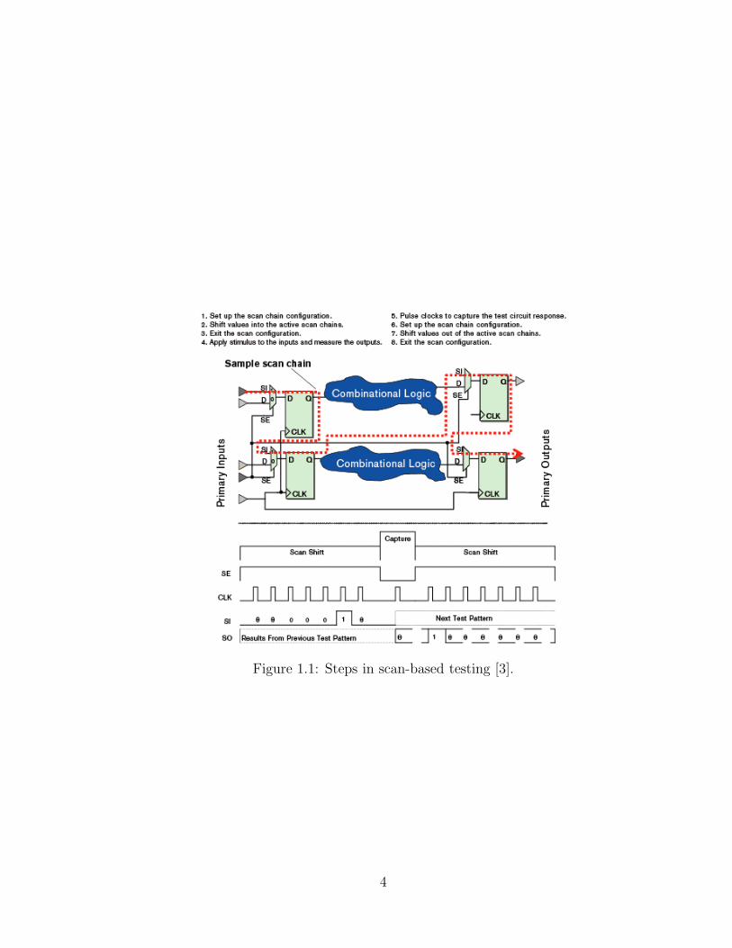
Figure 1.1: Steps in scan-based testing [3].

4

Typically, the number of scan cells is proportional to the design size. Thus, assuming

one scan cell per 20 gates, the total test time to apply 10,000 scan patterns at a 20-

MHz scan shift frequency will be roughly 312 million test cycles or equivalently 15.6

seconds. As designs grow larger, maintaining high test coverage becomes increasingly

expensive because the test equipment must store a prohibitively large volume of test

data and the test application time increases. Moreover, a very high and continually

increasing logic-to-pin ratio creates a test data transfer bottleneck at the chip pins.

Accordingly, the overall efficiency of any test scheme strongly depends on the method

employed to reduce the amount of test data.

The latest system-on-a-chip (SoC) designs integrate multiple ICs (microproces-

sors, memories, DSPs, and I/O controllers) on a single piece of silicon. SOCs consist

of several reusable embedded intellectual-property (IP) cores provided by third-party

vendors and stitched into designs by system integrators. Testing all these circuits

when they are embedded in a single device is far more difficult than testing them

separately. The testing time is determined by several factors, including the test data

volume, the time required to transfer test data to the cores, the rate at which the

test patterns are transferred (measured by the test data bandwidth and the ATE

channel capacity), and the maximum scan chain length. For a given ATE channel

capacity and test data bandwidth, reduction in test time can be achieved by reduc-

ing the test data volume and by redesigning the scan chains. While test data volume

reduction techniques can be applied to both soft and hard cores, scan chains cannot

5

be modified in hard (IP) cores.

Test patterns are usually generated and stored on workstations or high-performance

personal computers. The increased variety of ASICs and decreased production vol-

ume of individual types of ASICs require more frequent downloads of test data from

workstations to ATE. In addition, because of the sheer size of test sets for ASICs,

often as large as several gigabytes, the time spent to download test data from com-

puters to ATE is significant. The download from a workstation storing a test set

to the user interface workstation attached to an ATE is often accomplished through

a network. The download may take several tens of minutes to hours [4]. The test

set is then transferred from the user interface workstation of an ATE to the main

pattern memory through a dedicated high speed bus. The latter transfer usually

takes several minutes. The transfer of data from a workstation to an ATE is shown

in Figure 1.2.

While downloading a test set, the ATE is normally idle. The overall throughput

of an ATE is affected by the download time of test data and the throughput becomes

more sensitive to the download time with the increased variety of ASICs. One

common approach to improve the throughput of an ATE is to download the test

data of the next chip during the testing of a chip. This cuts down the effective

download time of test data, but the approach alone may not be sufficient. An ATE

may finish testing of the current chip before the download of the next test data is

completed.

6

ATE

Test Controller

Pattern Memory

Test Pattern Storage

CUT

~ hour

~ minutes

Figure 1.2: Download of test data to ATE [5].

ATE costs have been rising steeply. Achieving satisfactory SOC test quality at

an acceptable cost and with minimal effect on the production schedule is also be-

coming increasingly difficult. High transistor counts and aggressive clock frequencies

require expensive automatic test equipment (ATE). More important, these introduce

many problems into test development and manufacturing test that decrease product

quality, increase cost and time to market. A tester that can accurately test today’s

complex ICs costs several million dollars. According to the 1999 International Tech-

nology Roadmap for Semiconductors [6], the cost of a high-speed tester will exceed

$20 million by 2010, and the cost of testing an IC with conventional methods will

exceed fabrication cost.The increasing ratio of internal node count to external pin

count makes most chip nodes inaccessible from system I/O pins, so controlling and

observing these nodes and exercising the numerous internal states in the circuit un-

7

der test is difficult. ATE I/O channel capacity, speed, accuracy, and data memory

are limited. Therefore, design and test engineers need new techniques for decreasing

data volume.

Built-in self-test (BIST) has emerged as an alternative to ATE-based external

testing [7]. BIST offers a number of key advantages. It allows precomputed test sets

to be embedded in the test sequences generated by on-chip hardware. It supports

test reuse, at-speed testing, and protects intellectual property. While BIST is now

extensively used for memory testing, it is not as common for logic testing. This

is particularly the case for non-scan and partial-scan designs in which test vectors

cannot be reordered and application of pseudorandom vectors can lead to serious

bus contention problems during test application. Moreover, BIST can be applied

to SOC designs only if the IP cores in it are BIST-ready. BIST insertion in SOCs

containing these circuits maybe expensive and may require considerable redesign.

Test resource partitioning (TRP) offers a promising solution to these problems

by moving some test resources from ATE to chip [8]. One of the possible TRP

approaches is based on the use of test data compression and on-chip decompression,

hence reducing test data volume, decreasing testing time, and allowing the use

of slower testers without decreasing test quality. Test-data compression offers a

promising solution to the problem of reducing the test-data volume for SoCs. In

one approach, a precomputed test set TD for an IP core is compressed (encoded) to

a much smaller test set TE , which is stored in ATE memory. An on-chip decoder is

8

used for pattern decompression to obtain TD from TE during test application (See

Figure 1.3). Another approach is to introduce logic in the scan path at scan-in

and scan-out. Test data volume and test application time benefits are achieved by

converting data from a small scan interface at the design boundary to a wide scan

interface within the design. This approach enables significantly more scan chains in

the design than allowed by its signal interface [3].

Core

Core

Core

Core

Core

Core

Decoder Decoder Decoder

Decoder Decoder Decoder

SoC

Test Access Mechanism (TAM) ATE Memory (TE)

Test Head

Figure 1.3: Conceptual architecture for testing an SoC by storing the encoded testdata (TE) in ATE memory and decoding it using on-chip decoders [?].

A majority of bits in test patterns are unspecified. Prior to the rise of test data

volume and test application time, the typical industry practice was to randomly fill

the unspecified bits [9]. Test compression technology creatively discovers alternatives

for handling these randomly filled bits, which decreases test data volume and test

application time efficiency.

Because the goal of test compression is to increase the efficiency of scan test-

9

ing, this new technology provides better results without losing the existing benefits

of scan. However, not every test compression technique is compatible with scan

technology.

This work proposes a test vector compression scheme that is based on a reconfig-

urable broadcast scan approach that drives N scan chains using M tester channels.

Using direct compatibility analysis [10], test vectors are classified into ‘acceptable’

and ‘bottleneck’ vectors. Acceptable vectors are those that can be driven by M

tester channels while bottleneck vectors are those that cannot be driven by M chan-

nels. Acceptable vectors are partitioned into the smallest number of partitions in

such a way that all test vectors in a partition can be driven by M tester channels.

Each partition corresponds to a test configuration and thus minimizing the number

of partitions reduces the decoder complexity. Bottleneck vector are decomposed into

a small subset of test vectors each satisfying the tester channel constraint M, using

an efficient relaxation-based test vector decomposition technique [11]. Then, decom-

posed test vectors are partitioned minimizing the number of partitions. By varying

M with a given input test data set for a specified number of internal scan chains,

the proposed technique allows tradeoffs among test compression, area overhead and

test application time. Furthermore, the technique can take advantage of compacted

test sets to achieve high compression ratios with small test vector counts.

This thesis is organized as follows: Chapter 2 presents a review of existing tech-

niques for test data volume reduction. This is followed by description of the pro-

10

posed technique in Chapter 3. Experiments and analysis of results are presented in

Chapter 4. Chapter 5 concludes the thesis with mention of future work.

11

Chapter 2

Literature Survey

In this chapter, a review of existing work on scan-based test data volume reduction

is presented. This area has received considerable attention in the last five years.

As a result, a large number of techniques have been reported in literature and

commercial products from Electronic Design Automation tool vendors are available

that integrate test data compression into the overall IC design flow [12, 13].

In order to systematically present the vast number of techniques proposed, they

are classified into categories based on the underlying principles. Broadly speaking,

the proposed solutions can be classified into:

1. Test set compaction

2. Scan architectures

3. Test data compression

12

2.1 Test Set Compaction

Test set compaction is the process of reducing the number of test vectors in a

test set to the minimum while achieving the desired fault coverage. Finding the

smallest set is proven to be an NP-hard problem [14], therefore, heuristics are used

to find a reasonable solution [15]. There are two main categories of test compaction

techniques: static compaction and dynamic compaction. In static compaction, the

test set is reduced after it has been generated. On the other hand, it is reduced

during the generation process in dynamic compaction. Compaction is not discussed

in detail here as the focus of this work is test data compression. The gains in test

data volume reduction by using compaction alone are limited [16]. However, some

form of compaction is used implicitly or explicitly by many test data compression

techniques to reduce the number of distinct test vectors to be applied, thus achieving

greater compression as well as savings in test application time.

2.2 Scan Architectures

Several enhancements to the existing scan architecture have been proposed in the

literature for test volume, time and power reductions. Lee et al. [17] present a scan

broadcasting scheme where ATPG patterns are broadcasted to multiple scan chains

within a core or across multiple cores. The broadcast mode is used when the vectors

going into multiple chains are compatible. Illinois Scan Architecture (ISA) [18] was

13

introduced to reduce data volume and test application time by splitting a given scan

chain into multiple segments. Since a majority of the bits in ATPG patterns are

don’t care bits, there are chances that these segments will have compatible vectors

(not having opposite care bits in one location). In this case, all segments of a given

chain are configured in broadcast mode to read the same vector. This speeds up

the test vector loading time and reduces the data volume by a factor equivalent

to the number of segments. In case if the segments within a given scan chain

are incompatible, the test vector needs to be loaded serially by reconfiguring the

segments into a single long scan chain. The fact that a majority of the ATPG bits

(95-99%) [9] are don’t care bits makes ISA an attractive solution for data volume

and test time.

Huang and Lee [19] introduced a token scan architecture to gate the clock to

different scan segments while taking advantage of the regularity and periodicity of

scan chains. Another scheme for selective triggering of scan segments was proposed

by Sharifi et al. [20]. A novel scheme was presented by Sinanoglu and Orailoglu [21]

to reduce test power consumption by freezing scan segments that don’t have care

bits in the next test stimulus. By only loading the segments that have care bits,

test data volume, application time, and power consumption are all reduced at once.

Only one segment of the scan chain is controlled and observed at a time.

A reconfigurable scheme is introduced by Samaranayake et al. [22] that uses

mapping logic to control the connection of multiple scan chains. This increases

14

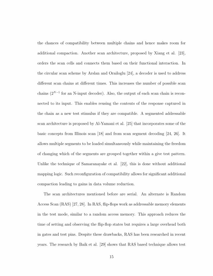
the chances of compatibility between multiple chains and hence makes room for

additional compaction. Another scan architecture, proposed by Xiang et al. [23],

orders the scan cells and connects them based on their functional interaction. In

the circular scan scheme by Arslan and Orailoglu [24], a decoder is used to address

different scan chains at different times. This increases the number of possible scan

chains (2N−1 for an N-input decoder). Also, the output of each scan chain is recon-

nected to its input. This enables reusing the contents of the response captured in

the chain as a new test stimulus if they are compatible. A segmented addressable

scan architecture is proposed by Al-Yamani et al. [25] that incorporates some of the

basic concepts from Illinois scan [18] and from scan segment decoding [24, 26]. It

allows multiple segments to be loaded simultaneously while maintaining the freedom

of changing which of the segments are grouped together within a give test pattern.

Unlike the technique of Samaranayake et al. [22], this is done without additional

mapping logic. Such reconfiguration of compatibility allows for significant additional

compaction leading to gains in data volume reduction.

The scan architectures mentioned before are serial. An alternate is Random

Access Scan (RAS) [27, 28]. In RAS, flip-flops work as addressable memory elements

in the test mode, similar to a random access memory. This approach reduces the

time of setting and observing the flip-flop states but requires a large overhead both

in gates and test pins. Despite these drawbacks, RAS has been researched in recent

years. The research by Baik et al. [29] shows that RAS based technique allows test

15

application time and data volume to be greatly reduced, besides over 99% power

reduction. However, it shows that this method compromises the test cost with a high

hardware overhead and the practicality of RAS architecture implementation were

not addressed. A modified RAS scheme has been described by Arslan and Orailoglu

[30] in which the captured response of the previous patterns in the flip-flops is used

as a template and modified by a circular shift for subsequent pattern. Mudlapur et

al. presents a unique RAS cell architecture [31, 32] that aims to minimize the routing

complexity. Another novel scan architecture called Progressive Random Access Scan

(PRAS) [33] and the associated test application methods have been proposed. It

has a structure similar to static random access memory. Test vector ordering and

Hamming distance reduction are proposed to minimize the total number of write

operations for a given test set [33, 34]. Partitioned Grid Random Access Scan

[35] method uses multiple PRAS grids with partitioning. This method achieves

much greater test application time reductions compared to multiple serial scans

with additional test pins. A test compaction technique has also been used with

RAS. In parallel random access virtual scan (PRAVS) architecture [36]. Along with

a X-tolerant compactor, PRAVS, achieves greater test data/time reductions than

conventional RAS.

Recently, compression schemes utilizing RAS architecture have been proposed.

Cocktail Scan [37], a hybrid method unlike the LFSR-based hybrid BIST, adopts a

two-phase approach to perform scan test in which all test data are supplied from the

16

ATE. However, for test patterns, instead of supplying the long inefficient pseudo-

random patterns generated by LFSRs, a set of carefully-chosen efficient seed patterns

are supplied to perform a “cycle” random scan test in the first phase, achieving a

considerable high fault coverage. At the second phase, deterministic patterns are

supplied to detect remaining faults. These patterns are applied in the RAS fashion

and they are reordered and compressed with some proposed strategies to reduce data

volume, number of bit flips, and consequently, test energy. A compression/scan co-

design approach by Hu et al. [38] achieves the goal of simultaneously reducing test

data volume, power dissipation and application time by exploiting the characteristics

of both variable-to-fixed run-length coding and random access scan architectures,

along with a heuristic algorithm for an optimal arrangement of scan cells.

2.3 Test Data Compression

The various test data compression schemes for scan-based testing, utilizing either

single or multiple scan chains architectures, can be classified into the following broad

categories:

1. Code-based schemes that use some form of coding, such as run-length encod-

ings, Huffman encodings, or some variants and combinations of these, often

borrowed from existing data compression methods and modified to suit the

requirements of test data compression. Dictionary based compression is also

17

included under this category.

2. Linear-decompression-based schemes that decompress data using only linear

operations (LFSRs and XOR networks).

3. Broadcast-scan-based schemes rely on broadcasting the same values to multiple

scan chains, also known as width or horizontal compression.

4. Compression techniques utilizing arithmetic structures such as subtractors or

multipliers.

5. Hybrid schemes that use more than one of the above techniques.

Compression techniques can also be classified as: (i) those that utilize the struc-

tural information about the circuit under test by relying on ATPG/fault simulation,

(ii) techniques that do not require any structural information but require ATPG tai-

lored to the technique, and (iii) those that can operate on any given test set. This

type of classification is not focused upon in this survey.

Code-based approaches assign a codeword C(v) to a sequence of test data v (an

input block). For instance, v could be 10011101, and C(v) could be 110. Then, if

110 is transmitted from the tester, an on-chip decoder would generate the sequence

10011101 and apply it to the circuit under test. Most compression techniques of

this type compress TD without requiring any structural information about the em-

bedded cores. Proposed compression schemes include statistical coding [39, 40],

18

selective Huffman coding [41], mixed run-length and Huffman coding [42], Golomb

coding [43], frequency-directed run-length (FDR) coding [44], geometric shape-based

encoding [45], alternating run-length coding using FDR [46], extended FDR coding

[47], MTC coding [48], variable-input Huffman coding (VIHC) coding[49], nine-

coded compression technique [50], Burrows-Wheeler transform based compression

[?], arithmetic coding [51], mutation codes [52], packet-based codes [53] and non-

linear combinational codes [54]. A multi-level Huffman coding scheme that utilizes

a LFSR for random filling has been proposed by Kavousianos et al. [55] while Po-

lian et al. [56] proposes use of an evolutionary heuristic with a Huffman code based

technique. A scheme based on MICRO (Modified Input reduction and CompRessing

One block) code is proposed by Chun et al. [57] that uses an input reduction tech-

nique, test set reordering, and one block compression with a novel mapping scheme

to achieve compression with a low area overhead. This technique does not require

cyclic scan registers (CSR), which is used by many of the code-based techniques

mentioned above that compress the difference of scan vectors. Ruan and Katti [58]

presents a data-independent compression method called pattern run-length coding.

This compression scheme is a modified run-length coding that encodes consecu-

tive equal/complementary patterns. The software-based decompression algorithm

is small and requires very few processor instructions.

A block merging based compression technique is proposed by Aiman [59] that

capitalizes on the fact that many consecutive blocks of the test data can be merged

19

together. Compression is achieved by storing the merged block and the number

of blocks merged. A compression scheme using multiple scan chains is proposed by

Hayashi et al. [60] based on reduction of distinct scan vectors (words) using selective

don’t-care identification. Each bit in the specified scan vectors is fixed to either a

0 or 1, and single/double length coding is used for test data volume reduction, in

which the code length for frequent scan vectors is shortened in a manner that the

code length for rare scan vectors is designed to be double of that for frequent ones.

A compression scheme extending run-length coding is presented by Doi et al. [61]

that employs two techniques: scan polarity adjustment and pinpoint test relaxation.

Given a test set for a full-scan circuit, scan polarity adjustment selectively flips the

values of some scan cells in test patterns. It can be realized by changing connections

between two scan cells so that the inverted output of a scan cell, Q’, is connected to

the next scan cell. Pinpoint test relaxation flips some specified 1s in the test patterns

to 0s without any fault coverage loss. Both techniques are applied by referring to a

gain-penalty table to determine scan cells or bits to be flipped.

Several dictionary-based compression methods have been proposed to reduce

test-data volume. Jas et al. [40] proposed a technique which encodes frequently

occurring blocks into variable-length indices using Huffman coding. Reddy et al.

used a dictionary with fixed-length indices to generate all distinct output vector [62].

Test-data compression techniques based on LZ77, LZW and test-data realignment

methods are proposed by Pomeranz and Reddy [63], Knieser et al. [64] and Wolff

20

and Papachristou [65], respectively. Li et al. proposed [66] a compression technique

using dictionary with fixed-length indices for multiple-scan chain designs. A hybrid

coding scheme, combining alternating run-length and dictionary-based encoding,

is proposed by Wurtenberger et al. [67], and another dictionary scheme based on

multiple scan chains architecture that uses a correction circuit [68]. Shi et al. [69]

uses dictionary-based encoding on single or sequences of scan-inputs.

The next class of techniques are ones using LFSR reseeding [70, 71, 72, 73, 74, 75].

The original test compression methodology using LFSR reseeding was proposed by

Koenemann [70]. A seed is loaded into an LFSR and then the LFSR is run in an

autonomous mode to fill a set of scan chains with a deterministic test pattern. If

the maximum length of each scan chain is L, then the LFSR is run for L cycles to

fill the scan chains. Different seeds generate different test patterns, and for a given

set of deterministic test cubes (test patterns where bits unassigned by ATPG are

left as don’t cares), the corresponding seeds can be computed for each test cube by

solving a system of linear equations based on the feedback polynomial of the LFSR.

The Embedded Deterministic Test method [76] uses a ring generator which is an

alternative linear finite state machine that offers some advantages over an LFSR.

Another group of compression techniques [77, 78] breaks the single long scan

chain down into multiple internal scan chains that can be simultaneously sourced.

Because the number of I/O pins available from the ATE is limited, a decompression

network is used to drive the internal scan chains with far fewer external scan chains.

21

But due to the asymmetry in size between the test vectors and the test responses,

a Multiple Input Signature Register (MISR) is used to compress the test responses

so that a test response can still be shifted out while the next test vector is being

shifted in. Such an architecture is known as the Multiple Scan Chain Architecture,

and the hardware overhead is the cost of the MISR plus the cost of the decompression

network, which ranges from a simple fanout based network to the relatively more

complicated XOR gates or MUXs based network. Most of these techniques are based

on what is known as width compression or horizontal compression, utilizing the idea

of scan chains compatibility as used in ILS. The idea of input compatibility was

first introduced in the context of width compression for BIST based test generation

process [10]. Width reduction for BIST has been achieved by merging directly and

inversely compatible inputs [10], by merging decoder (d)-compatible inputs [79],

and, finally, by merging combinational (C)-compatible inputs [80]. In the ILS [18],

a simple fanout based network is used. Though simple and low-cost, this type of

network is highly restrictive, as it forces the internal scan chains to receive the

exact same values. Therefore, to provide for both full fault coverage and adequate

compression, a separate serial shifting mode capable of bypassing the network is used

to test some of the faults. Other proposals can be seen as the logical extension to the

above approach. Inverters are coupled with fanouts to form the inverter-interconnect

based network in approach by Rao et al. [81]. An enhancement of the Illinois Scan

Architecture for use with multiple scan inputs is presented by Shah and Patel [82]

22

while Ashiouei et al. [83] presents a technique for balanced parallel scan to improve

ILS technique eliminating the need to scan vectors in serially. In the Scan Chain

Concealment approach [77], a pseudorandomly-built XOR network that is based

on Linear Feedback Shift Register (LFSR) is used. An improvement is shown by

Bayraktaroglu and Orailoglu [78], which constructs the network deterministically

from an initial set of test cubes. A similar approach has been proposed using a

ring generator, instead of an XOR network, to construct such a decompression

architecture [76].

Many multiple-scan architecture based compression schemes uses extra control

logic to reconfigure the decompression network [84, 54, 85]. For the price of some sig-

nificant amount of extra control hardware, these approaches can provide additional

flexibility in enhancing the compression ratio. Oh et al. [86] improves upon the

ILS compression technique using fan-out scan chains, creating a solution in which

dependencies caused by the fan-out scan chain structure do not interfere in the ap-

plication of test patterns. Conflicts across the fan-out scan chains are handled by

using prelude vectors whose purpose is not to detect faults but to resolve conflicts

in a test pattern. The number of prelude vectors is a function of the number of

conflicts in an individual test pattern: fewer prelude vectors for fewer conflicts, and

more prelude vectors for more conflicts. Therefore, it avoids the extreme solution of

serializing all the scan chains to resolve conflicts.

23

In Selective Low Care (SLC) scheme [87], the linear dependencies of the internal

scan chains are explored, and instead of encoding all the specified bits in test cubes,

only a smaller amount of specified bits are selected for encoding. It employs a Fan-

out Compression Scan Architecture (FCSCAN) [88], the basic idea of which is to

target the minority specified bits (either a 1 or 0) in scan slices for compression.

A compression scheme using reconfigurable linear decompressor has been pro-

posed [89]. A symbolic Gaussian elimination method to solve a constrained Boolean

matrix is proposed and utilized for designing the reconfigurable network. The pro-

posed scheme can be implemented in conjunction with any decompressor that has

a combinational linear network. In a scheme based on periodically alterable MUXs

[90], MUXs-based decompressor has multiple configurations to decode the input

information. The connection relations between the external scan-in pins and the

internal scan chains can be altered periodically. The periodic reconfiguration of the

mapping between the scan-in pins and the internal scan chains is done by changing

the control signals of the MUXs decompressor. Only a single input is required to

change the configurations. The scheme uses tailored ATPG along with a two-pass

patterns compaction. The scheme proposed in this work also uses idea of configu-

rations of MUXs to decompress groups of scan chains.

Schemes utilizing arithmetic structures include a reconfigurable serial multiplier

based scheme [91] in which test vectors are stored on the tester in a compressed

format by expressing each test vector as a product of two numbers. While performing

24

multiplication on these stored seeds in the Galois Field modulo 2 (GF (2)), the

multiplier states (i.e. the partial products) are tapped to reproduce the test vectors

and fill the scan chains. A multiple scan chains compression scheme based on the

principle of storing differences between vectors instead of the vectors themselves is

presented by Dalmasso et al. [16]. Differences (Di) between the original N bits

vectors (Vi) coded using M bits with M < N are obtained. If {V1, V2, . . .} be the

initial test sequence and Di = Vi+1 − Vi modulo 2N be the differences between the

two successive vectors Vi and Vi+1, then Di is stored in the ATE instead of Vi+1 when

Di can be coded on M bits, otherwise Vi+1 is stored using ⌈NM⌉ × M bits memory

words. The compressed stored sequence is thus composed of M bits words and these

represent either a difference between two original vectors, or the ⌈N

M⌉ subpart of an

N bits original vector.

A hybrid scheme that uses horizontal compression combined with dictionary

compression is proposed by Li et al. [92] where the output of horizontal compression

is further compressed with a dictionary scheme using both fixed and variable length

indices.

The compression scheme proposed in this work uses the idea of input compati-

bility [80] to compress multiple scan chains test data via width reduction [10, 79]. It

tries to overcome the bottlenecks that prevent greater achievable compression. The

next chapter presents the details of the proposed technique.

25

Chapter 3

Proposed Compression Algorithms

3.1 Introduction

In this work we propose a test data compression technique that utilizes a multiple

scan chains configuration. This configuration is shown in Figure 3.1(a). The input

test set consists of nV scan test vectors, each vector configured into N scan chains of

length L each. The output of the compression algorithm is shown in Figure 3.1(b).

It contains nV ′ test vectors, where nV ′ ≥ nV , each encoded using M representative

scan chains of length L. These vectors, called representative vectors, are grouped

into nP partitions. Figure 3.2 shows the block diagram of the hardware and CUT,

where M is the number of ATE scan input channels and N denotes the number

of scan chains internal to the core feeding the scan cells. In this configuration,

N ≫ M , i.e., the compressed input test data is composed of a much smaller number

26

n Vte

st p

atte

rns

n V’te

st p

atte

rns

in n

Ppa

rtiti

ons

1XX0

1X0X

0XXX

X0X1

X0X1

0X0X

0XXX

X1X0

1X0X

X00X

00XX

XX01

1X0X

X0X1

010X

X11X

100X

XX01

N Scan Chains M Input Channels

(a) (b)

L fli

p flo

ps

L fli

p flo

ps

Figure 3.1: (a) Multiple scan chains test vectors configuration used by the compres-sion algorithm, (b) Output of the compression algorithm.

of M input scan chains relative to the decompressed output having N scan chains.

It should be noted that N is a parameter given as an input to the compression

algorithm along with M , which is the desired target.

The proposed technique uses the idea of input compatibility [80] to compress mul-

tiple scan chains test data via input width reduction [10, 79] and tries to overcome

the bottlenecks that prevent greater achievable compression. The main contribu-

tions of the proposed technique are:

1. It uses an approach that partitions the test data into groups of scan vectors

such that multiple scan chains of these scan vectors are maximally compatible

amongst them, resulting in fewer scan chains required to compress the whole

27

M x N Decompression Network

Internal Scan Chains (N x L)

ATE Channels (M)

L

Figure 3.2: Block diagram of the decompression hardware and CUT with inputsand outputs.

test set. Partitioning enables achieving high compression without requiring

’bloated’ test sets consisting of a very large number of test vectors with a very

few specified bits [93, 94].

2. Those scan vectors (labeled as bottleneck vectors) that limit achieving a de-

sired M are decomposed using an efficient relaxation-based test vector de-

composition technique [11] in an incremental manner so as to increase the

unspecified bits, resulting in better compression of the resulting relaxed vec-

tors.

3. The technique is parameterized so that the tradeoff between the desired com-

pression, hardware costs and final test set size can be explored by obtaining a

number of solutions for a given input test set.

28

Hence, the goal of the proposed technique is to achieve the user specified com-

pression target, using test set partitioning and relaxation-based decomposition of

bottleneck vectors, if such a solution exists for the given test data set. In this

chapter, the proposed compression technique is presented. Before the actual algo-

rithms are explained, the main concepts used such as compatibility based merging,

partitioning of test vectors into groups that satisfy the desired compatibility, and

relaxation based decomposition of test vectors, are explained with simple examples.

3.2 Multiple Scan Chains Merging Using Input

Compatibility

The concept of scan chain compatibility and the associated fan-out structure have

been utilized in a number of papers [78, 18, 82, 22] since the broadcast scan ar-

chitecture was presented by Lee et al. [95]. It is also referred to as ’test width

compression’ [77, 68]. Let b(k, i, j) denote the data bit that is shifted into the jth

flip-flop of ith scan chain for the kth test vector. The compatibility of a pair of scan

chains is defined as follows. The ith1 scan chain and the ith2 scan chain are mutually

compatible if for any k, where 1 ≤ k ≤ nV ′ , and j, where 1 ≤ j ≤ L, b(k, i1, j) and

b(k, i2, j) are either equal to each other or at least one of them is a don’t-care. A

conflict graph is then constructed from the test data and graph coloring is used to

obtain the number of ATE channels needed. The conflict graph G contains a vertex

29

for each scan chain. If two scan chains are not compatible, they are connected by

an edge in G. A vertex coloring of G yields the minimum number of ATE channels

required to apply the test cubes with no loss of fault coverage (in the graph coloring

solution a minimum number of colors is determined to color the vertices such that no

two adjacent vertices are assigned the same color). Vertices in G that are assigned

the same color represent scan chains that can be fed by the same ATE channel via

a fan-out structure. This procedure is illustrated using Figure 3.3. In this example,

the number of scan chains N = 8, and the scan chain length L = 4. A conflict graph

consisting of 8 vertices is first determined. The coloring solution for the conflict

graph is also shown; three colors are used to color three sets of vertices: {1}, {2, 4,

5, 7}, {3, 6, 8}. Consequently, three ATE channels are needed to feed the test data

for the 8 scan chains, and the fan-out structure is shown in Figure 3.3. Since the

graph coloring problem is known to be NP-complete, a heuristic technique is used

in this work.

3.3 Partitioning of Test Vectors

In section 3.2, it was shown how the input compatibility analysis is applied over the

complete test set to obtain a reduced number of representative scan chains resulting

in reduced data volume. Based on this, the following key observations can be made:

• Given a number of parallel scan chains of a scan vector, the compatibility

30

1 X 0 1 X X 1 0 X 0 X X 0 X 0 X X X 0 1 X 0 X X 0 0 X X X 1 X 1

0 X 0 0 X 0 X X X X 1 X X X X 1 1 0 X X 0 1 0 1 X 0 X 0 0 X 0 X

1 1 X X 1 0 1 X X X 1 X X 1 X 1 1 X 0 1 X X 1 0 0 1 X 1 X X X X

(a)

1

4

6 7

8

5

3

2

(b)

1 1 0 X 0 X X 1 0 0 0 1

0 0 0 X X 1 1 0 1 X 0 X

1 1 0 X X 1 1 1 0 0 1 X

(c)

(d)

5 6 7 8 1 2 3 4

1 2 3

Figure 3.3: Width compression based on scan chain compatibilities; (a) Test cubes,(b) Conflict graph, (c) Compressed test data based on scan chain compatibility, (d)Fan-out structure.

31

analysis gives a reduced number of representative parallel scan chains if the

given parallel chains are compatible amongst themselves.

• The extent of compatibility achieved depends upon how many bits are specified

per scan vector. The lesser the specified bits, the lesser the conflicts, resulting

in greater compatibility between the set of parallel chains.

• The compatibility analysis can be applied to parallel scan chains of a single

vector or a set of vectors. Depending upon the extent of specified bits present,

the amount of conflict tends to increase the longer the chains (or columns) are.

The length of each column is determined by the number of bits per column

per vector multiplied by the total number of test vectors being considered for

the analysis.

• Compatibility analysis per vector gives the lower bound on achievable repre-

sentative parallel scan chains for a given test set for a specified number of

parallel scan chains per vector.

When the compatibility analysis is done per vector, the resulting number of

representative scan chains and the configuration of compatible groups may vary

among the different vectors in a test set depending upon the amount of specified bits

present and their relative positions in each vector. Even if most vectors individually

lend themselves favorably to compression using compatibility analysis, the gains

become less due to the increased conflicts when multiple vectors are considered

32

together. Thus, when many vectors are being considered together, their combination

can limit the compression of the test set and in the worst case this may allow no

compression at all. From these observations, it is intuitively clear that greater

compression can be achieved if the test vectors are partitioned into bins such that

all vectors in a given bin satisfy a targeted M when considered together during

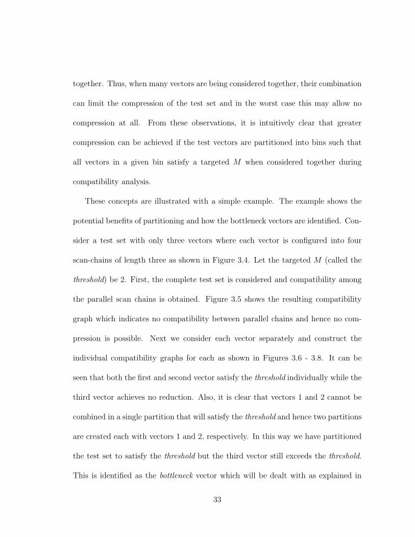
compatibility analysis.

These concepts are illustrated with a simple example. The example shows the

potential benefits of partitioning and how the bottleneck vectors are identified. Con-

sider a test set with only three vectors where each vector is configured into four

scan-chains of length three as shown in Figure 3.4. Let the targeted M (called the

threshold) be 2. First, the complete test set is considered and compatibility among

the parallel scan chains is obtained. Figure 3.5 shows the resulting compatibility

graph which indicates no compatibility between parallel chains and hence no com-

pression is possible. Next we consider each vector separately and construct the

individual compatibility graphs for each as shown in Figures 3.6 - 3.8. It can be

seen that both the first and second vector satisfy the threshold individually while the

third vector achieves no reduction. Also, it is clear that vectors 1 and 2 cannot be

combined in a single partition that will satisfy the threshold and hence two partitions

are created each with vectors 1 and 2, respectively. In this way we have partitioned

the test set to satisfy the threshold but the third vector still exceeds the threshold.

This is identified as the bottleneck vector which will be dealt with as explained in

33

Section 3.4.

Vector SC1 SC2 SC3 SC4 1

0 X 0

0 1 0

1 1 X

X 1 1

2

0 X 1

1 X 0

X 0 1

X 1 0

3

0 0 0

1 X 0

X 1 1

X 0 1

Figure 3.4: Example test set to illustrate the algorithm

SC1

SC2

SC4

SC3

Figure 3.5: Conflict graph for the complete test set

3.4 Relaxation Based Decomposition of Test Vec-

tors

It may be the case that many vectors do not achieve the desired M (threshold) due

to the relatively large number of specified bits present and their conflicting relative

positions. The idea of test vector decomposition (TVD) [15] can be used to increase

the number of unspecified bits per vector. TVD is the process of decomposing a

34

SC1

SC2

SC4

SC3

Figure 3.6: Conflict graph for vector 1

SC1

SC2

SC4

SC3

Figure 3.7: Conflict graph for vector 2

test vector into its atomic components. An atomic component is a child test vector

that is generated by relaxing its parent test vector for a single fault f . That is, the

child test vector contains the assignments necessary for the detection of f . Besides,

the child test vector may detect other faults in addition to f . For example, consider

the test vector tp = 010110 that detects the set of faults Fp = {f1, f2, f3}. Using

the relaxation algorithm by El-Maleh and Al-Suwaiyan [11], tp can be decomposed

into three atomic components, which are t1 = (f1, 01xxxx), t2 = (f2, 0x01xx), and

t3 = (f3, x1xx10). Every atomic component detects the fault associated with it and

may accidentally detect other faults. An atomic component cannot be decomposed

any further because it contains the assignments necessary for detecting its fault.

35

SC1

SC2

SC4

SC3

Figure 3.8: Conflict graph for vector 3

To achieve the desired compression ratio, the bottleneck vector can be decomposed

into subvectors in the following manner. The atomic components for each fault

detected by the bottleneck vector is obtained. These atomic components are then

merged incrementally creating a new subvector from the parent bottleneck vector

until this subvector just satisfies the desired M . As many subvectors are created

this way until all the faults detected by the parent are covered. These subvectors

are made members of the existing partitions or new partitions are created to achieve

the desired M as per compatibility analysis. The goal at this stage is to minimize

the number of vectors resulting from this relaxation-based decomposition while also

minimizing the total number of partitions. To achieve this, an efficient approach is

to first fault simulate the more specified representative vectors in existing partitions

and drop all faults detected. The bottleneck vectors are decomposed to target only

those faults that remain undetected. The role of TVD in increasing compression is

illustrated with a simple example.

Consider the bottleneck vector identified in the earlier example. Suppose that

36

Vector SC1 SC2 SC3 SC4 3

0 0 0

1 X 0

X 1 1

X 0 1

3a

0 X 0

X X 0

X 1 1

X X 1

3b

X 0 X

1 X X

X X 1

X 0 1

Figure 3.9: Decomposition of vector 3 into two vectors 3a and 3b

this vector is decomposed into two vectors 3a and 3b as shown in Figure 3.9, each

detecting only a subset of faults detected by the original vector. The compatibility

graphs of these vectors are shown in Figures 3.10 and 3.11. The decomposed vectors

satisfy the threshold. Now these decomposed vectors can be merged with the existing

partitions or new partitions can be created if required.

SC1

SC2

SC4

SC3

Figure 3.10: Conflict graph for vector 3a

3.5 Proposed Compression Algorithms

The objective of the proposed algorithm is to compress the test test using M tester

channels while minimizing the increase in test size (due to decomposition) and to-

37

SC1

SC2

SC4

SC3

Figure 3.11: Conflict graph for vector 3b

tal partitions, while maintaining the original fault coverage (%FC). The increase

in test set size increases the test application time and after a certain point even

decreases compression, while the number of distinct partitions increases the area

overhead of the decoder. To minimize the decomposition needed, the approach used

in the algorithm is to minimize the number of undetected faults associated with each

subsequently decomposed bottleneck vector as it directly affects the amount of de-

composition required: the fewer the undetected faults, the lesser the decomposition

required to derive new acceptable test vectors. Since a representative vector derived

from broadcasted scan values is more specified than the original test vector, it detects

more faults. To benefit from this fact, all acceptable vectors present in the input

test set are partitioned and faults detected by the representative vectors obtained

after partitioning are dropped. Then, during bottleneck vector decomposition, each

derived subvector is partitioned and its representative vector is fault simulated to

drop newly detected faults before any further decomposition. However, in this ap-

proach the fault coverage depends upon the representative vectors and if they are

38

modified, the fault coverage changes. This may happen because a partition changes

as new vectors are made members of existing partitions. If the partition attains a

different configuration of compatibility classes to accommodate a new vector, all the

representative vectors previously created for existing members of this partition need

to be updated. The consequence is that some faults that are detected by the old set

of representative vectors may become undetected. This can happen for faults that

are essential in the original test set and detected by a bottleneck vector. When such

faults are covered by some other representative vector, they are dropped and not

considered during bottleneck vector’s decomposition. However, the representative

vector may be modified after the bottleneck vector has been decomposed, making

the fault undetected, unless it is detected surreptitiously during the remaining pass

by some representative vector. Surreptitious detection is usually possible for non-

essential faults, but not for essential ones. Two approaches can be used to deal with

this problem: (i) either not to allow any previous essential fault detection to change

while partitioning, or (ii) allow faults detection to be disturbed but address it by

creating new vectors if needed. These two approaches can give different solutions in

terms of total partitions created and the final test vectors count. The first approach

tends to create more partitions as a vector will not be included in an existing par-

tition if there is disturbance of any previous essential fault detection. On the other

hand, the second approach may create more new vectors but has a potential to give

fewer total partitions as a new vector is most likely to be included in an existing par-

39

tition because of high percentage of don’t cares present. Three variations have been

proposed based on these two strategies to explore the solutions space that results

due to the choice between creating a new vector or a new partition. The difference

among these variations is in the partitioning step when decomposing the bottleneck

vectors and specifically in the choice that needs to be made between creating a new

partition for a newly created vector or using an existing partition with a chance of

reduced fault coverage and then creating new vector(s) to make up for it. It should

be noted that the initial partitioning of acceptable vectors does not have this issue

since acceptable vectors are not recreated while partitioning.

When the second approach is taken, to minimize the increase in vectors that

are created to make up for reduced fault coverage, a merging step is attempted

before creating any new vectors. In this merging step, the atomic component for

a dropped fault is tested for merging with an existing partitioned subvector with

the same originating parent vector as for this atomic component. Since this merge

changes the subvector being merged with, the partition to which this subvector

belongs to is recolored and all member representative vectors renewed and checked

for any fault dropping. The merge is only successful if no dropping of essential faults

occurs. If unsuccessful, the dropped fault is covered by creating new subvector. In

this step as well, the increase in number of vectors is minimized by combining the

components for a group of faults with the same parent vector as a common subvector

satisfying the coloring threshold.

40

Another variation is proposed that has the potential to give fewer partitions and

also reduced total vectors, especially for cases with a high percentage of bottlenecks.

In this variation, new acceptable vectors having greater don’t cares are obtained by

relaxing for all essential faults. These are partitioned and representative vectors

are fault simulated as just discussed. Similarly, the bottlenecks are decomposed

and partitioned for essential faults only. The detection of non-essential faults is left

to the more specified representative vectors and any undetected faults are finally

handled in the last two steps as described before.

Having discussed the basis of the technique and its variations, the overall algo-

rithm is now given and then the details of the critical substeps and the algorithm’s

variations are elaborated subsequently in the referenced subsections.

3.5.1 Algorithm

1. Fault simulate test set to mark essential and non-essential faults.

2. Analyze the compatibility of each test vector to get its representative scan

chains (representative count). M is the maximum representative count that is

acceptable, called the threshold.

3. Include vectors with representative count > threshold in set bottleneck, other-

wise in set acceptable.

4. Partition acceptable vectors using the initial partitioning algorithm (Section

41

3.5.2)

5. Get representative test vectors for all partitioned test vectors, fault simulate

them and drop all detected faults.

6. Incrementally decompose each bottleneck vector into subvector(s) for all its

undetected faults. Partition each subvector and fault simulate its representa-

tive vector to drop faults before any further decomposition of the bottleneck

vector (Section 3.5.3).

7. Fault simulate the set of all representative vectors to check %FC. If %FC <

original, generate atomic components for all undetected faults and attempt

merging them with existing partitions (Section 3.5.4).

8. For remaining undetected faults, atomic components for these faults are merged

into the smallest set of subvectors satisfying the threshold and are partitioned

without disturbing existing fault detection.

The algorithm does not perform any merging based compaction or random fill of

don’t cares in the representative vectors because the compatibility constraints can

be violated.

42

3.5.2 Initial Partitioning

If there are acceptable vectors present in the test set, an initial partitioning is

performed that will allow representative vectors to be created and fault simulated

so that faults can be dropped before handling the bottleneck vectors. The heuristic

used for partitioning initial acceptable vectors is as follows:

1. The acceptable vectors, are sorted on their representative count in descending

order.

2. The first vector in the sorted list is made a member of the first (default)

partition.

3. The compatibility of the next test vector is analyzed together with members

of existing partition(s), testing the available partitions list in order. If the

test vector and the existing test vectors in a partition can be M colored, it is

included in the partition. Otherwise, the next partition is tested.

4. If the test vector fails to be partitioned with any of the existing partitions, a

new partition is created.

5. Steps 3-4 are repeated until all acceptable test vectors are processed.

Test vectors with higher representative counts are attempted first as they tend to

be more conflicting with other test vectors and have less degree of freedom. However,

test vectors with lesser representative counts have more X’s and have higher chances

43

of fitting in existing partitions before any new partitions are created, thus leading

to fewer total partitions.

3.5.3 Bottleneck Vector Decomposition and Partitioning

Bottleneck test vectors are decomposed and partitioned according to the following

steps:

1. Select an undetected fault from the fault list of the bottleneck vector and add

its atomic component to a new subvector.

2. Select the next undetected fault from the list and merge its atomic component

with the subvector. Determine the representative count of the subvector.

3. If M is not exceeded and there are undetected faults remaining, go to step 2.

4. Undo the last merge if the threshold was exceeded and perform partitioning

of the created subvector.

5. Get the representative vectors of the modified partition and fault simulate

them to drop all detected faults.

6. If the current bottleneck vector has remaining undetected faults, goto step 1.

A subvector is first tested for inclusion in a partition by applying the existing com-

patibility graph of a partition to the subvector. If it succeeds, current fault detection

44

is not disturbed. If this fails with all partitions, partitioning with recoloring is at-

tempted in a similar manner as explained in section 3.5.2. But in this case, the

problem of fault coverage loss (Section 3.5) has to be addressed. As mentioned

earlier, three variations are proposed to address this issue. Before details of these

variations are given, some terms related to fault detection need to be mentioned in

order to clearly explain and justify the approach taken.

Since the algorithm relies on representative vectors created during partitioning

for providing the required fault coverage, at any instant, the current test set is

composed of all representative vectors and the unprocessed bottleneck vectors, if

any. The term ’disturbed’ is used for a fault to imply that it was detected before

the latest change to the set of representative vectors took place and now it is not

detected by any representative vector in any partition. Furthermore, since the test

set is being recreated using representative vectors, the essential and non-essential

status of each fault keeps changing dynamically as each new representative vector is

created. However, it should be noted that the algorithm relies on the initial essential

and non-essential status of each fault, i.e., based on the initial test set. Based on

this, all originally non-essential faults are treated as easy to detect faults and are

not cared for during decomposition and partitioning if being disturbed. This is

done because these faults are assumed to have a high probability of surreptitious

detection by representative vectors and this fact is used to minimize any new vectors

and partitions created to deal with these faults.

45

The details of the implemented variations are now given under the headings

Algorithm IA, IB and II.

Algorithm IA

This variation uses the approach of not disturbing the faults that are essential and

whose detecting vector has been processed. If including the newly created subvector

in a partition results in such a disturbance, another partition is tried. Finally,

a new partition is created if no existing partition satisfies the conditions. The

case of essential faults of currently being processed bottleneck vector needs special

mention. In this variation, the currently being processed bottleneck vector is treated

as ’partially processed’ in terms of all faults that were checked in step 2 of bottleneck

vector decomposition (Section 3.5.3). In other words, those essential faults detected

by the currently being processed bottleneck vector that have already been checked

are not allowed to be disturbed. Non-essential faults on the other hand are ignored

as they have a high probability of surreptitious detection. However, in case of

non-detection of any non-essential fault, the last two steps in the algorithm (Section

3.5.1) can handle these faults as explained in Section 3.5.4. This variation minimizes

the number of new vectors created at the expense of more partitions.

46

Algorithm IB

Except for a slight variation, this algorithm is based on the same approach as Algo-

rithm IA. In this variation the currently being processed bottleneck vector is marked

’unprocessed’ until all its faults have been covered. In other words, any fault that

is detected by the currently being processed bottleneck vector is allowed to be dis-

turbed. To ensure that a disturbed essential fault of the current bottleneck vector

is not dropped, the current vector’s fault list is checked from the beginning each

time during each subsequent decomposition. Non-essential faults are handled in the

same manner as in Algorithm IA. This variation may give fewer partitions in some

cases due to the slightly relaxed partitioning criteria but may also lead to creating

new vectors.

Algorithm II

This variation is essentially an unrestricted version of Algorithm IB. It allows any

fault to be disturbed when partitioning subvectors of bottleneck vectors. In this

algorithm, all partitions are tested and the partition that gives the minimum distur-

bance is selected. All the disturbed faults that are not covered even after processing

of all bottleneck vectors are taken care of in the last two steps, i.e., component

merging (Section 3.5.4) or by creating new vectors. Algorithm II attempts to mini-

mize partitions by relaxing the partitioning criteria at the expense of creating more

vectors.

47

3.5.4 Merging of Atomic Components with Partitioned Sub-

vectors

To restore fault coverage without creating any new vectors and partitions, for each

undetected fault the following steps are done:

1. Get atomic component for the undetected fault and locate all partitioned sub-

vector(s) that are derived from the same parent vector as this component.

2. Merge the atomic component with a subvector and recolor that partition.

3. If M is exceeded try next available subvector. Otherwise, regenerate represen-

tative vectors according to the new compatibility configuration of the partition

and check for any fault detection disturbance.

4. If merging is unsuccessful, try next available subvector.

When merging fails, step 8 in the test compression algorithm (Section 3.5.1) is

performed by grouping the atomic components of undetected faults into the smallest

set of subvectors satisfying the threshold. Then, these subvectors are partitioned

without any fault detection disturbance.

3.5.5 Algorithm III: Essential Faults First Approach

The idea behind this variation is to begin with more relaxed vectors by processing

initially the essential faults in case of both the acceptable and bottleneck vectors.

48

Intuitively, this can lead to fewer partitions due to the greater flexibility in partition-

ing owing to fewer specified bits in each vector being partitioned. In this algorithm,

instead of starting with the given test vectors, new vectors are created that detect

only the essential faults. From these new vectors, the acceptable and bottleneck

vectors are identified as already explained in Section 3.5. The decomposition of

bottleneck vectors and the associated subvector partitioning only considers the es-

sential faults. The coverage of non-essential faults is left to surreptitious detection

by the more specified representative vectors initially. However, the undetected non-

essential faults are taken care of by using merging (Section 3.5.4) or by additional

vectors creation at the end. During the decomposition and partitioning of bottleneck

vectors for essential faults, Algorithms IA is used as the goal is to ensure detection

of essential faults and minimize vectors created and the associated partitions.

3.6 Illustrative Example

In this section, a simple example is presented to illustrate the various steps of the

algorithm and highlight the different outcomes that may result when different varia-

tions are used, specifically Algorithm IA and II. Suppose that the number of vectors

are 4, the chosen scan configuration is N = 8 and the targeted M is 3. The test set

and the compatibility analysis details are given in Table 3.1. The acceptable vectors

1 and 2 are partitioned using the initial partitioning algorithm resulting in a single

49

partition. The representative vectors created and the faults dropped are shown in

Table 3.2. The bottleneck vector 3 is decomposed to create the new subvector 3a.

A new partition needs to be created for this subvector as it cannot fit in partition

1. No further decomposition of vector 3 is required because all its other faults have

already been detected by the set of all representative vectors. Table 3.3 shows the

subvector 3a, its representative vector and the faults detected. The bottleneck vec-

tor 4 is now decomposed for all undetected faults into the subvector 4a as shown

in Table 3.4. This vector can be partitioned in partition 1 with recoloring while

partition 2 cannot accommodate it. If partition 1 is selected, the new partition con-

figuration and the faults detected are shown in Table 3.5. However, it can be seen

that with this partitioning, the essential fault f9 is now disturbed and its detecting

vector 3 has already been processed. Algorithms IA and IB do not allow this, thus, if

Algorithm IA/IB is being used, partition 2 is tested and since this partition cannot

accommodate the subvector 4a, a new partition 3 is created with the subvector 4a.

All the faults have been detected and no further decomposition is required. On the

other hand, if algorithm II is employed, the disturbed essential fault f9 needs to be

covered. In this case, first merging is attempted with the partitioned subvector 3a

but, it fails as the threshold (M) is exceeded. So, a new subvector 3b is created

that is partitioned with partition 2 without recoloring due to a high percentage of

Xs. Hence, more vectors are created when Algorithm II is employed compared to

Algorithm IA/IB in this case while Algorithm IA/IB creates more partitions.

50

Vectors

Colors Compatibility Classes

Faults Detected

Acceptable

0 X 1 X 0 1 0 1 X 1 X X X 1 1 x 1 1 0 1 X X x x

2 {1,2,4,5,7}, {3,6,8}

f1, f2, f3, f4

Yes

0 1 X X X 0 X X X X 1 1 0 X X 1 1 X X X X 1 1 X

2 {2,5,7}, {1,3,4,6,8}

f1, f4, f5, f6

Yes

0 0 1 X 1 0 1 1 1 0 1 0 X 0 X X X 0 X 1 0 X 0 1

4 {1}, {2,6}, {3,5,7}, {4,8}

f1, f3, f7, f8, f9, f10, f11, f13

No

X 1 0 1 1 X 0 1 0 X X 1 0 1 0 1 0 1 1 0 0 0 0 1

5 {1,5}, {2,8}, {3}, {4,6},

{7}

f5, f11, f12, f13, f14,

f15, f16

No

Table 3.1: The test set and compatibility analysis details for the example.

Representative Vectors 1 and 2

Compatibility Classes

Colors Faults Covered

0 X 1 X 0 1 0 1 1 1 1 1 1 1 1 1 1 1 0 1 1 0 1 0 0 1 0 1 0 0 0 0 0 1 1 1 0 1 0 1 1 X 1 X 1 1 1 1

{1,5,7}, {2,4}, {3,6,8}

3

f1, f2, f3, f4, f5, f6, f7, f9

Table 3.2: Details of partition 1.

Subvector 3a and its Rep. vector

Compatibility Classes

Colors Faults Covered

X 0 1 X 1 0 1 1 1 X 1 0 X 0 X X X 0 X 1 X X 0 1 1 0 1 1 1 0 1 1 1 0 1 0 0 0 1 0 0 0 0 1 1 0 0 1

{1,3,7}, {2,6}, {4,5,8}

3

f1, f3, f7, f8, f10, f11, f13

Table 3.3: Details of partition 2.

Vector 4 and its Subvector 4a

Compatibility Classes

Colors Faults Covered

X 1 0 1 1 X 0 1 0 X X 1 0 1 0 1 0 1 1 0 0 0 0 1

X 1 0 1 1 X X X 0 X X 1 X X 0 X X X 1 X 0 X X 1

{1,3,7},

{2,4,6,8}, {5}

3

f5, f12, f14, f15, f16

Table 3.4: Decomposition of bottleneck vector 4.

51

Representative Vectors 1,2 & 4a

Colors Compatibility Classes

Faults Detected

0 0 1 0 0 1 0 1 X 1 1 X 1 1 1 1 1 1 0 1 1 0 1 0 0 1 0 0 1 0 1 0 1 0 1 1 0 1 0 1 1 1 1 1 1 1 1 1 1 1 0 1 1 0 1 0 1 0 X 1 0 X 0 X 1 0 1 1 0 1 0 1

3

{2,5,7}, {3,6,8}, {1,4}

f1, f2, f3, f4, f5, f6, f7, f8, f12, f14, f15, f16

Table 3.5: Details of modified partition 1.

3.7 Decompression Hardware

The decompression hardware for compatibility based compression is simply a fan-

out structure as shown in Figure 3.3(d). The decompression hardware required to

support partitioning of the test set can be realized by MUXs. Essentially, since

each partition has a different set of compatibility classes, it requires it’s own fan-

out structure. The MUXs allow different fan-out structures to be switched in as

required. Thus, the number of MUXs required is equal to the number of fan-out

scan chains feeding the core, i.e., N . The number of inputs on each of these MUXs

is equal to the number of partitions i.e. nP . A counter (S) changes the select lines of

the MUXs when a partition changes. The enable input of this counter is controlled

by another counter (T), which is loaded with the partition size to support the non-

uniform partition sizes. The T counter is loaded with the size of partition when

the first vector of a partition is input and then it keeps decrementing with each

52

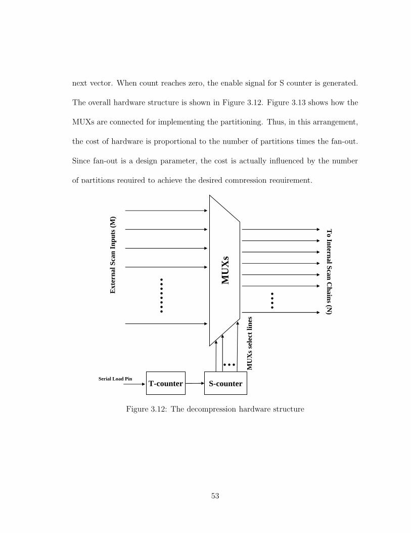
next vector. When count reaches zero, the enable signal for S counter is generated.

The overall hardware structure is shown in Figure 3.12. Figure 3.13 shows how the

MUXs are connected for implementing the partitioning. Thus, in this arrangement,

the cost of hardware is proportional to the number of partitions times the fan-out.

Since fan-out is a design parameter, the cost is actually influenced by the number

of partitions required to achieve the desired compression requirement.

MU

Xs

S-counterT-counter

To Internal Scan C

hains (N)

Ext

erna

l Sca

n In

puts

(M

)

MU

Xs

sele

ct li

nes

Serial Load Pin

Figure 3.12: The decompression hardware structure

53

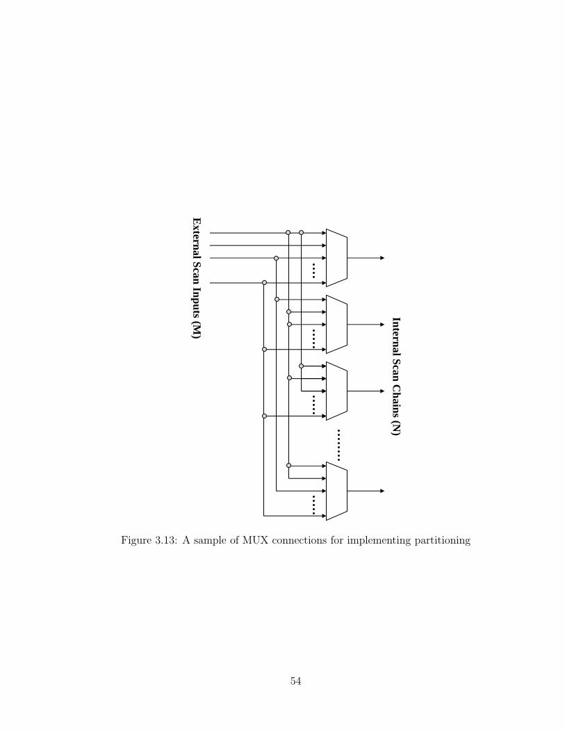
Internal Scan Chains (N

)

External Scan Inputs (M

)

Figure 3.13: A sample of MUX connections for implementing partitioning

54

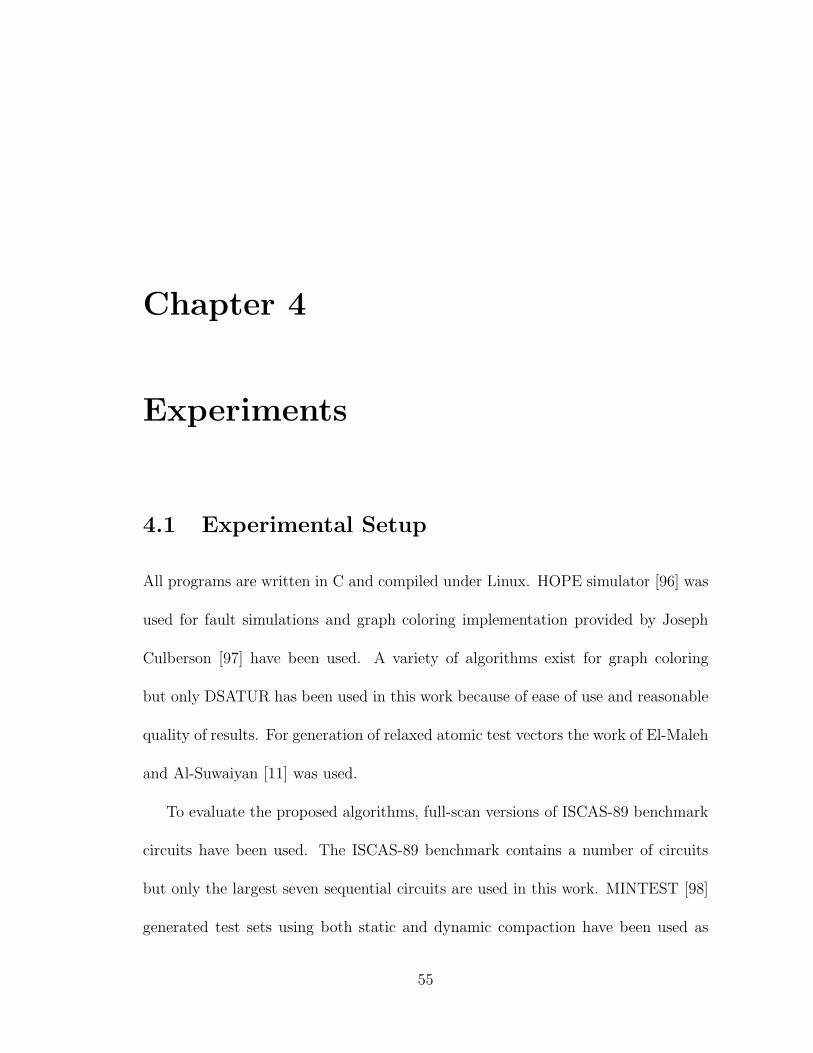
Chapter 4

Experiments

4.1 Experimental Setup

All programs are written in C and compiled under Linux. HOPE simulator [96] was

used for fault simulations and graph coloring implementation provided by Joseph

Culberson [97] have been used. A variety of algorithms exist for graph coloring

but only DSATUR has been used in this work because of ease of use and reasonable

quality of results. For generation of relaxed atomic test vectors the work of El-Maleh

and Al-Suwaiyan [11] was used.

To evaluate the proposed algorithms, full-scan versions of ISCAS-89 benchmark

circuits have been used. The ISCAS-89 benchmark contains a number of circuits

but only the largest seven sequential circuits are used in this work. MINTEST [98]

generated test sets using both static and dynamic compaction have been used as

55

Table 4.1: Details of ISCAS-89 benchmarks and test sets usedMINTEST Static compacted MINTEST Dynamic compacted

Test Case #FFs %FC #TV %DC TD #TV %DC TD

s5378 214 99.13 97 74.14 20758 111 72.62 23754s9234 247 93.48 105 70.29 25935 159 73.01 39273s13207 700 98.46 233 93.36 163100 236 93.15 165200s15850 611 96.68 94 80.96 57434 126 83.56 76986s35932 1763 89.81 12 36.68 21156 16 35.3 28208s38417 1664 99.47 68 67.36 113152 99 68.08 164736s38584 1464 95.85 110 80.72 161040 136 82.28 199104

input test data for compression. The static compacted test sets have been relaxed

using a bit-wise relaxation approach [11] to obtain a large percentage of don’t care

bits that are representative of today’s industrial test cases. These test sets have been

used for the detailed results presented in this chapter. The dynamic compacted test

sets are used for comparison with other work. Since the relaxation algorithm used in

this work requires fully specified test vectors, fully specified version of both test sets

are used for generating the atomic test vectors. The details of benchmark circuits

and test sets used are given in Table 4.1. The columns #FFs, %FC, #TV, %DC

and TD respectively imply no. of scan flip-flops in the benchmark, the fault coverage

percentage of the test set, total number of test vectors, percentage of don’t care bits

present and the test data volume in bits.

4.2 Methodology

As discussed in section 3.1, the proposed compression technique requires the number

of scan chains N as an input parameter along with the desired compression target

56

in terms of number of external ATE channels M . Theoretically, any value of N can

be used, however, actual constraints on routing dictate the maximum allowed N

value for a given circuit [22]. As shown in Section 4.3, a larger N generally results

in better compression in general due to fewer conflicts in compatibility analysis.

The value of N that gives the greatest compression can be obtained empirically.

The experimentation results are presented for N approaching 100 and 200 scan

chains for the largest five circuits and N approaching 64 scan chains for the smaller

circuits. These values enable comparison with existing work, which use similar input

configurations. For each input configuration, the desired M value is varied such that

the behavior of the algorithm with respect to the number of partitions created and

final test vector count can be observed for a wide range of compression targets for

each test case. There is, however, a limit on the minimum value of M permitted

with a given test set and chosen N . This is determined by the minimum number of

colors required to color the atomic component of any fault in the list.

The characteristics of test data configurations for varying scan chain lengths

are presented first. Next, results and analysis of the proposed technique and a

comparison among the variants is given. Comparison with existing work is then

presented followed by a discussion of hardware costs.

57

4.3 Test Data Characteristics

Before discussing the results of the proposed algorithms, analysis of the test sets

with different scan chain length configurations is presented. Figures 4.1 - 4.7 show

the number of bottleneck vectors with decreasing M , obtained through compatibility

analysis of the seven test cases for different scan chain length configurations. The

compression ratio (CR%) is defined as:

CR% =nV × L × N − nV ′ × L × M

nV × L × N= 1 −

nV ′ × M

nV × N= 1 −

M

N×

nV ′

nV

Note that decreasing the M corresponds to increasing the compression ratio. It is

observed that the bottleneck vectors increase with both increasing compression and

scan chain lengths, thus requiring more decomposition for targeting a smaller M .

To show the impact of partitioning, Figure 4.8 shows the achievable compression

without partitioning at each scan chain length configuration for all test cases. It can

be seen that little or no compression is achieved except for very small scan chain

lengths. Figure 4.9 shows the achievable compression with partitioning at different

scan chain lengths with M set equal to the maximum representative count in the

test set so that no test vector decomposition is required. The required partitions

are shown in Figure 4.10. Significant compression is achieved by using partitioning,

especially at small chain lengths. By using test vector decomposition, compression

58

70 74 78 82 86 90 94 982

6 0

20

40

60

80

100

Bot

tlene

ck V

ecto

rs

Compression

Scan Chain Length

s5378

23456

Figure 4.1: Bottleneck vectors with respect to scan chain length and desired com-pression for s5378.

70 72 74 76 78 80 82 84 86 88 90 92 94 96 98

2

4

6

0

20

40

60

80

100

120

Bot

tlene

ck V

ecto

rs

CompressionScan Chain

Length

s9234

23456

Figure 4.2: Bottleneck vectors with respect to scan chain length and desired com-pression for s9234.

59

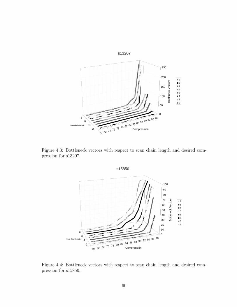
70 72 74 76 78 80 82 84 86 88 90 92 94 96 98

2

46

80

50

100

150

200

250

Bot

tlene

ck V

ecto

rs

Compression

Scan Chain Length

s13207

23456789

Figure 4.3: Bottleneck vectors with respect to scan chain length and desired com-pression for s13207.

70 72 74 76 78 80 82 84 86 88 90 92 94 96 98

2

4

68

0

10

20

30

40

50

60

70

80

90

100

Bot

tlene

ck V

ecto

rs

Compression

Scan Chain Length

s15850

23456789

Figure 4.4: Bottleneck vectors with respect to scan chain length and desired com-pression for s15850.

60

7074 78 82 86 90 94 98

2

6

10

14

18

0

2

4

6

8

10

12

Bot

tlene

ck V

ecto

rs

Compression

Scan Chain Length

s35932

234567891011121314151617181920

Figure 4.5: Bottleneck vectors with respect to scan chain length and desired com-pression for s35932.

70 74 78 82 86 90 94 98

2

6

10

14

18

0

10

20

30

40

50

60

Bottleneck Vectors

Compression

Scan Chain Length

s38417

2345678910111213141516171819

Figure 4.6: Bottleneck vectors with respect to scan chain length and desired com-pression for s38417.

61

70

74 78 82 86 90 94 98

2

6

10

14

0

20

40

60

80

100

Bottleneck Vectors

Compression%

Scan Chain Length

s38584

234567891011121314151617

Figure 4.7: Bottleneck vectors with respect to scan chain length and desired com-pression for s38584.

can be further improved as shown in Section 4.4. Color histograms of vectors in each

test set for two different scan chain lengths used are given in Appendix 5. These are

helpful in estimating the range of compression that can be expected.

62

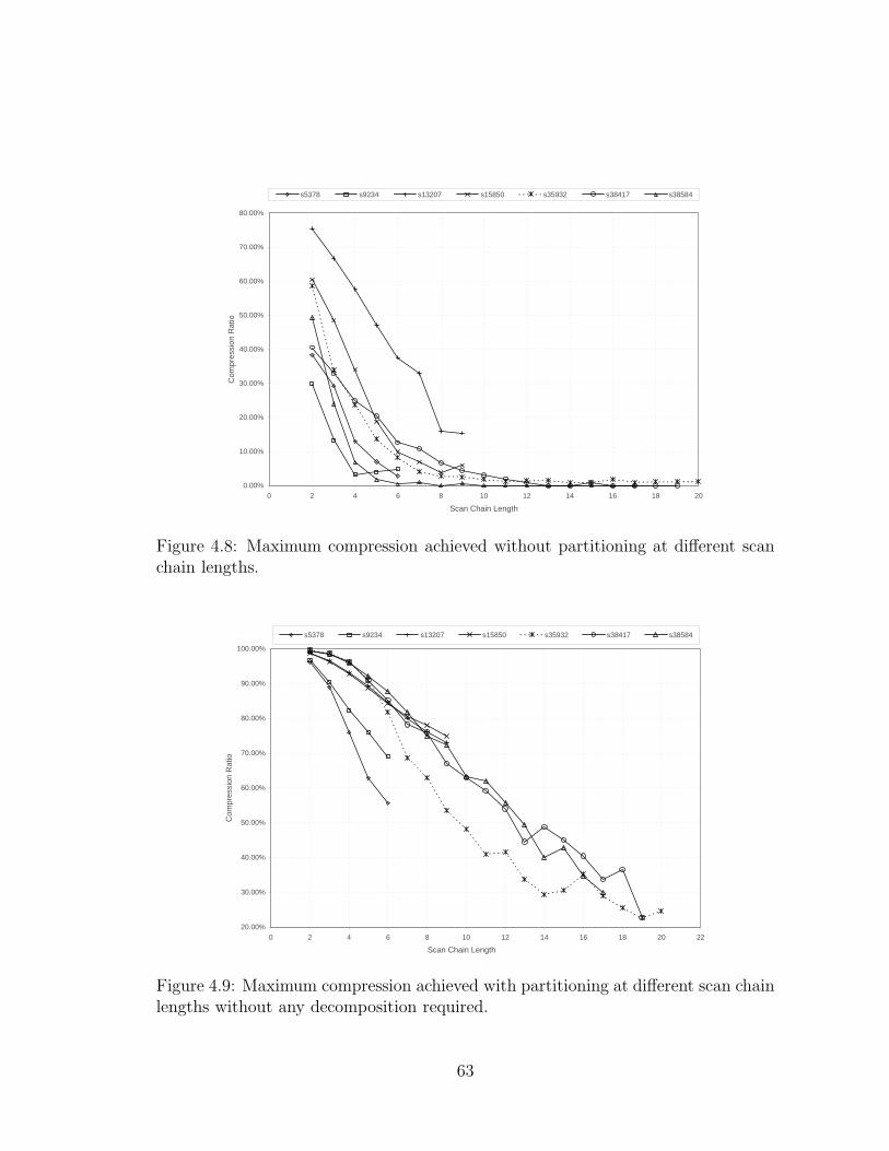
0.00%

10.00%

20.00%

30.00%

40.00%

50.00%

60.00%

70.00%

80.00%

0 2 4 6 8 10 12 14 16 18 20

Scan Chain Length

Com

pres

sion

Rat

io

s5378 s9234 s13207 s15850 s35932 s38417 s38584

Figure 4.8: Maximum compression achieved without partitioning at different scanchain lengths.

20.00%

30.00%

40.00%

50.00%

60.00%

70.00%

80.00%

90.00%

100.00%

0 2 4 6 8 10 12 14 16 18 20 22

Scan Chain Length

Com

pres

sion

Rat

io

s5378 s9234 s13207 s15850 s35932 s38417 s38584

Figure 4.9: Maximum compression achieved with partitioning at different scan chainlengths without any decomposition required.

63

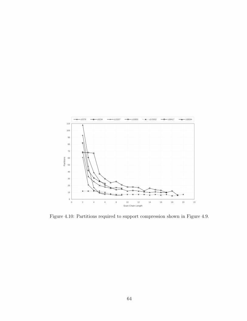
0

10

20

30

40

50

60

70

80

90

100

110

0 2 4 6 8 10 12 14 16 18 20 22

Scan Chain Length

Par

titio

ns

s5378 s9234 s13207 s15850 s3-5932 s38417 s38584

Figure 4.10: Partitions required to support compression shown in Figure 4.9.

64

4.4 Results and Discussion

The results for test cases are given in Tables 4.2 - 4.13. Each table shows results

of the four algorithm variations for the given scan chain length. The columns nB,

n′

V , nP and CR% give the number of bottleneck vectors, the final test vector count,

the number of partitions and the compression ratio, respectively. The highest com-

pression that is achieved without any increase in test vectors is shown underlined

while the overall highest compression achieved is shown in bold for all four varia-

tions. With increasing compression, there is invariably an increase in the number of

partitions required because of increased conflicts among the vectors when colored to-

gether, owing to a stricter constraint on the desired number of colors. Furthermore,

as decomposition creates more vectors, these may require new partitions to satisfy

the constraint. However, note that the test vectors count does not increase till a

certain point even though the decomposition of bottleneck vectors takes place. This

happens when a bottleneck vector(s) is decomposed only into a single vector because

a portion of its faults are already covered by other representative vectors. It can also

be observed that with decreasing M , the resulting compression increases until the

increase in test set size overcomes any gains from reduced M . The test case s35932

shows an irregular change in compression due to the small number of total vectors

such that any increase in vectors due to decomposition has a pronounced effect on

overall compression achieved. After the point where the decrease in M overcomes

65

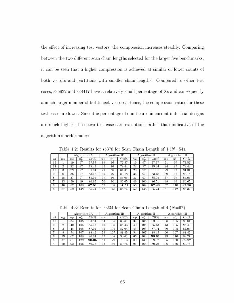
the effect of increasing test vectors, the compression increases steadily. Comparing

between the two different scan chain lengths selected for the larger five benchmarks,

it can be seen that a higher compression is achieved at similar or lower counts of

both vectors and partitions with smaller chain lengths. Compared to other test

cases, s35932 and s38417 have a relatively small percentage of Xs and consequently

a much larger number of bottleneck vectors. Hence, the compression ratios for these

test cases are lower. Since the percentage of don’t cares in current industrial designs

are much higher, these two test cases are exceptions rather than indicative of the

algorithm’s performance.

Table 4.2: Results for s5378 for Scan Chain Length of 4 (N=54).Algorithm IA Algorithm IB Algorithm II Algorithm III

M nB nP n′

VCR% nP n′

VCR% nP n′

VCR% nP n′

VCR%

12 1 19 97 77.57 19 97 77.57 19 97 77.57 21 97 77.5711 2 22 97 79.44 22 97 79.44 22 97 79.44 24 97 79.4410 3 29 97 81.31 29 97 81.31 29 97 81.31 29 97 81.319 6 36 97 83.18 36 97 83.18 36 97 83.18 39 97 83.188 18 37 97 85.05 37 97 85.05 37 97 85.05 37 97 85.057 23 50 99 86.65 50 99 86.65 49 100 86.51 49 99 86.656 46 57 108 87.51 57 108 87.51 56 109 87.40 57 110 87.28

5 67 52 148 85.74 52 148 85.74 52 148 85.74 51 142 86.32

Table 4.3: Results for s9234 for Scan Chain Length of 4 (N=62).Algorithm IA Algorithm IB Algorithm II Algorithm III

M nB nP n′

VCR% nP n′

VCR% nP n′

VCR% nP n′

VCR%

10 1 34 105 83.81 34 105 83.81 34 105 83.81 38 105 83.819 2 40 105 85.43 40 105 85.43 40 105 85.43 43 105 85.438 3 45 105 87.04 45 105 87.04 45 105 87.04 50 105 87.047 8 54 107 88.45 54 107 88.45 54 107 88.45 60 107 88.456 13 67 108 90.01 67 108 90.01 66 108 90.01 73 116 89.275 37 81 129 90.05 81 129 90.05 80 130 89.97 85 130 89.97

4 70 92 166 89.76 92 166 89.76 91 166 89.76 96 166 89.76

66

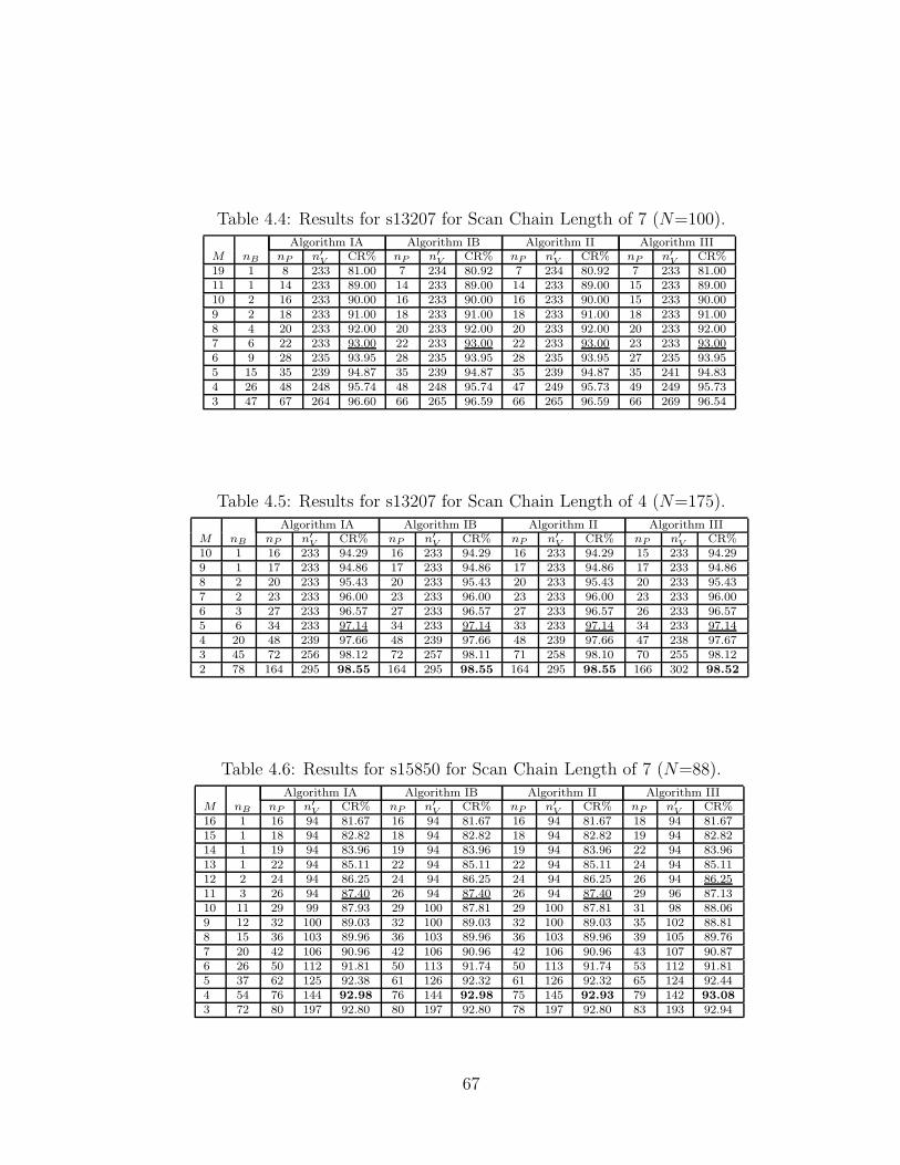
Table 4.4: Results for s13207 for Scan Chain Length of 7 (N=100).Algorithm IA Algorithm IB Algorithm II Algorithm III

M nB nP n′

VCR% nP n′

VCR% nP n′

VCR% nP n′

VCR%

19 1 8 233 81.00 7 234 80.92 7 234 80.92 7 233 81.0011 1 14 233 89.00 14 233 89.00 14 233 89.00 15 233 89.0010 2 16 233 90.00 16 233 90.00 16 233 90.00 15 233 90.009 2 18 233 91.00 18 233 91.00 18 233 91.00 18 233 91.008 4 20 233 92.00 20 233 92.00 20 233 92.00 20 233 92.007 6 22 233 93.00 22 233 93.00 22 233 93.00 23 233 93.006 9 28 235 93.95 28 235 93.95 28 235 93.95 27 235 93.955 15 35 239 94.87 35 239 94.87 35 239 94.87 35 241 94.834 26 48 248 95.74 48 248 95.74 47 249 95.73 49 249 95.733 47 67 264 96.60 66 265 96.59 66 265 96.59 66 269 96.54

Table 4.5: Results for s13207 for Scan Chain Length of 4 (N=175).Algorithm IA Algorithm IB Algorithm II Algorithm III

M nB nP n′

VCR% nP n′

VCR% nP n′

VCR% nP n′

VCR%

10 1 16 233 94.29 16 233 94.29 16 233 94.29 15 233 94.299 1 17 233 94.86 17 233 94.86 17 233 94.86 17 233 94.868 2 20 233 95.43 20 233 95.43 20 233 95.43 20 233 95.437 2 23 233 96.00 23 233 96.00 23 233 96.00 23 233 96.006 3 27 233 96.57 27 233 96.57 27 233 96.57 26 233 96.575 6 34 233 97.14 34 233 97.14 33 233 97.14 34 233 97.144 20 48 239 97.66 48 239 97.66 48 239 97.66 47 238 97.673 45 72 256 98.12 72 257 98.11 71 258 98.10 70 255 98.122 78 164 295 98.55 164 295 98.55 164 295 98.55 166 302 98.52

Table 4.6: Results for s15850 for Scan Chain Length of 7 (N=88).Algorithm IA Algorithm IB Algorithm II Algorithm III

M nB nP n′

VCR% nP n′

VCR% nP n′

VCR% nP n′

VCR%

16 1 16 94 81.67 16 94 81.67 16 94 81.67 18 94 81.6715 1 18 94 82.82 18 94 82.82 18 94 82.82 19 94 82.8214 1 19 94 83.96 19 94 83.96 19 94 83.96 22 94 83.9613 1 22 94 85.11 22 94 85.11 22 94 85.11 24 94 85.1112 2 24 94 86.25 24 94 86.25 24 94 86.25 26 94 86.2511 3 26 94 87.40 26 94 87.40 26 94 87.40 29 96 87.1310 11 29 99 87.93 29 100 87.81 29 100 87.81 31 98 88.069 12 32 100 89.03 32 100 89.03 32 100 89.03 35 102 88.818 15 36 103 89.96 36 103 89.96 36 103 89.96 39 105 89.767 20 42 106 90.96 42 106 90.96 42 106 90.96 43 107 90.876 26 50 112 91.81 50 113 91.74 50 113 91.74 53 112 91.815 37 62 125 92.38 61 126 92.32 61 126 92.32 65 124 92.444 54 76 144 92.98 76 144 92.98 75 145 92.93 79 142 93.08

3 72 80 197 92.80 80 197 92.80 78 197 92.80 83 193 92.94

67

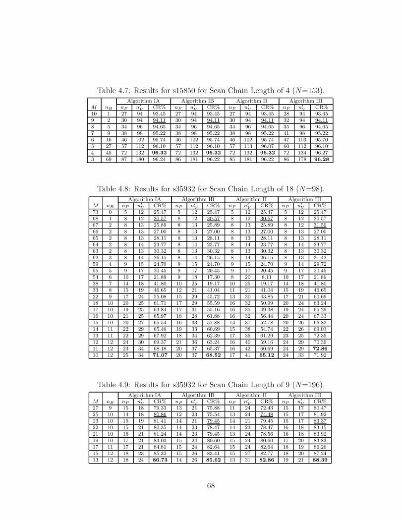
Table 4.7: Results for s15850 for Scan Chain Length of 4 (N=153).Algorithm IA Algorithm IB Algorithm II Algorithm III

M nB nP n′

VCR% nP n′

VCR% nP n′

VCR% nP n′

VCR%

10 1 27 94 93.45 27 94 93.45 27 94 93.45 28 94 93.459 2 30 94 94.11 30 94 94.11 30 94 94.11 32 94 94.118 5 34 96 94.65 34 96 94.65 34 96 94.65 35 96 94.657 9 38 98 95.22 38 98 95.22 38 98 95.22 41 98 95.226 16 46 102 95.74 46 102 95.74 46 102 95.74 47 103 95.705 27 57 112 96.10 57 112 96.10 57 113 96.07 60 112 96.104 45 72 132 96.32 72 132 96.32 72 132 96.32 72 134 96.273 69 87 180 96.24 86 181 96.22 85 181 96.22 86 178 96.28

Table 4.8: Results for s35932 for Scan Chain Length of 18 (N=98).Algorithm IA Algorithm IB Algorithm II Algorithm III

M nB nP n′

VCR% nP n′

VCR% nP n′

VCR% nP n′

VCR%

73 0 5 12 25.47 5 12 25.47 5 12 25.47 5 12 25.4768 1 8 12 30.57 8 12 30.57 8 12 30.57 8 12 30.5767 2 8 13 25.89 8 13 25.89 8 13 25.89 8 12 31.5966 2 8 13 27.00 8 13 27.00 8 13 27.00 8 13 27.0065 2 8 13 28.11 8 13 28.11 8 13 28.11 8 13 28.1164 2 8 14 23.77 8 14 23.77 8 14 23.77 8 14 23.7763 2 8 13 30.32 8 13 30.32 8 13 30.32 8 13 30.3262 3 8 14 26.15 8 14 26.15 8 14 26.15 8 13 31.4259 4 9 15 24.70 9 15 24.70 9 15 24.70 9 14 29.7255 5 9 17 20.45 9 17 20.45 9 17 20.45 9 17 20.4554 6 10 17 21.89 9 18 17.30 8 20 8.11 10 17 21.8938 7 14 18 41.80 10 25 19.17 10 25 19.17 14 18 41.8033 8 15 19 46.65 12 21 41.04 11 21 41.04 15 19 46.6522 9 17 24 55.08 15 29 45.72 13 30 43.85 17 21 60.6918 10 20 25 61.71 17 29 55.59 16 32 50.99 20 24 63.2417 10 19 25 63.84 17 31 55.16 16 35 49.38 19 24 65.2916 10 21 25 65.97 18 28 61.88 16 32 56.44 20 24 67.3315 10 20 27 65.54 16 33 57.88 14 37 52.78 20 26 66.8214 11 22 29 65.46 19 33 60.69 15 38 54.74 22 26 69.0313 11 22 29 67.92 18 34 62.39 17 35 61.29 23 25 72.3512 12 24 30 69.37 21 36 63.24 16 40 59.16 24 29 70.3911 12 23 34 68.18 20 37 65.37 16 42 60.69 24 29 72.86

10 12 25 34 71.07 20 37 68.52 17 41 65.12 24 33 71.92

Table 4.9: Results for s35932 for Scan Chain Length of 9 (N=196).Algorithm IA Algorithm IB Algorithm II Algorithm III

M nB nP n′

VCR% nP n′

VCR% nP n′

VCR% nP n′

VCR%

27 9 15 18 79.33 13 21 75.88 11 24 72.43 15 17 80.4725 10 14 18 80.86 12 23 75.54 13 24 74.48 15 17 81.9223 10 15 19 81.41 14 21 79.45 14 21 79.45 15 17 83.3722 10 15 21 80.35 14 23 78.47 14 23 78.47 16 18 83.1521 10 16 21 81.24 14 23 79.45 13 24 78.56 16 18 83.9219 10 17 21 83.03 15 24 80.60 15 24 80.60 17 20 83.8317 11 17 21 84.81 15 24 82.64 15 24 82.64 18 19 86.2615 12 18 23 85.32 15 26 83.41 15 27 82.77 18 20 87.2413 12 18 24 86.73 14 26 85.62 13 31 82.86 19 21 88.39

68

Table 4.10: Results for s38417 for Scan Chain Length of 17 (N=98).Algorithm IA Algorithm IB Algorithm II Algorithm III

M nB nP n′

VCR% nP n′

VCR% nP n′

VCR% nP n′

VCR%

32 7 40 68 67.31 40 68 67.31 40 68 67.31 40 68 67.3130 9 44 68 69.35 44 69 68.90 42 69 68.90 42 68 69.3528 11 48 68 71.39 48 69 70.97 47 68 71.39 47 68 71.3926 18 52 70 72.66 52 70 72.66 51 73 71.48 51 69 73.0524 27 57 73 73.68 57 73 73.68 57 73 73.68 57 73 73.6822 37 62 80 73.56 62 80 73.56 60 80 73.56 60 78 74.22

20 46 64 88 73.56 64 88 73.56 63 89 73.26 63 89 73.2618 56 66 102 72.42 66 102 72.42 65 105 71.60 65 102 72.4216 61 69 117 71.88 67 120 71.15 67 125 69.95 67 116 72.1215 63 69 124 72.06 69 126 71.60 67 129 70.93 67 125 71.83

Table 4.11: Results for s38417 for Scan Chain Length of 9 (N=185).Algorithm IA Algorithm IB Algorithm II Algorithm III

M nB nP n′

VCR% nP n′

VCR% nP n′

VCR% nP n′

VCR%

37 1 36 68 79.99 36 68 79.99 36 68 79.99 35 68 79.9935 2 41 68 81.07 41 68 81.07 41 68 81.07 37 68 81.0732 3 46 68 82.69 46 69 82.44 46 69 82.44 43 68 82.6929 6 53 68 84.31 53 68 84.31 53 68 84.31 50 68 84.3125 12 58 68 86.48 58 68 86.48 57 69 86.28 60 68 86.4822 28 66 74 87.05 66 74 87.05 63 75 86.88 66 70 87.75

18 53 67 94 86.54 67 100 85.68 67 100 85.68 67 95 86.4014 65 72 133 85.19 69 137 84.74 68 138 84.63 69 131 85.4111 67 71 180 84.25 71 184 83.90 72 185 83.81 72 180 84.25

Table 4.12: Results for s38584 for Scan Chain Length of 15 (N=98).Algorithm IA Algorithm IB Algorithm II Algorithm III

M nB nP n′

VCR% nP n′

VCR% nP n′

VCR% nP n′

VCR%

56 0 11 110 42.62 11 110 42.62 11 110 42.62 12 110 42.6251 1 13 110 47.75 13 110 47.75 13 110 47.75 14 110 47.7541 2 16 110 57.99 16 110 57.99 16 110 57.99 18 110 57.9939 5 18 110 60.04 16 112 59.31 16 112 59.31 19 110 60.0425 7 26 110 74.39 25 112 73.92 25 112 73.92 28 110 74.3919 10 34 112 80.18 32 114 79.82 32 115 79.65 35 111 80.3617 12 37 112 82.27 36 113 82.11 36 113 82.11 38 112 82.2715 13 43 112 84.35 41 114 84.07 41 114 84.07 43 113 84.2112 21 52 115 87.15 50 118 86.81 50 119 86.70 53 115 87.1510 25 59 115 89.29 59 115 89.29 58 119 88.92 62 115 89.29

Table 4.13: Results for s38584 for Scan Chain Length of 8 (N=183).Algorithm IA Algorithm IB Algorithm II Algorithm III

M nB nP n′

VCR% nP n′

VCR% nP n′

VCR% nP n′

VCR%

35 1 19 110 80.87 18 111 80.70 18 111 80.70 19 110 80.8732 2 20 110 82.51 20 111 82.35 20 111 82.35 20 110 82.5129 4 21 110 84.15 21 111 84.01 21 111 84.01 23 110 84.1521 7 29 110 88.52 28 112 88.32 28 111 88.42 29 110 88.5214 10 43 110 92.35 42 111 92.28 42 113 92.14 44 111 92.2810 19 57 113 94.39 57 115 94.29 56 115 94.29 58 112 94.448 27 71 114 95.47 71 115 95.43 70 118 95.31 76 112 95.556 47 96 121 96.39 96 121 96.39 94 121 96.39 94 120 96.42

4 104 123 186 96.30 128 190 96.22 121 194 96.15 119 189 96.24

69

The focus of comparison among the variations is each algorithm’s response to

increasing bottleneck vectors with increasing compression target. As discussed in

Section 3.5, the approach used to decompose bottlenecks and partition the subvec-

tors determine the final scan vectors count, number of partitions and ultimately the

actual compression ratio. This is the differentiating factor in the four variations.

The results of the first three variations are nearly identical in most cases except for

slight differences at very low M values. Among these three variations, Algorithm IA

achieves the lowest final test vector counts while Algorithms IB and II tradeoff test

vector counts for smaller number of partitions, though the differences in number of

vectors and partitions are not drastic. In a few cases, Algorithm IA achieves the

lowest in both partitions and vector counts. This is the case when new vector(s)

need to be created to handle the disturbed faults in Algorithms IB/II and these new

vectors also require new partition(s), thus leading to more vectors and partitions

compared to Algorithm IA.

Compared to the first three variations, the performance of Algorithm III is in-

ferior or at best just comparable except at very low M values, at which point the

compression curve has crossed the optimal point. Algorithm III results in more par-

titions and vectors in cases where many new vectors need to be created to handle

the non-essential faults. Furthermore, these new vectors may not fit in the existing

partitions, resulting in more new partitions. However, Algorithm III performs much

better in test cases s35932 and s38417 where it achieves the highest compression with

70

the least partitions. In these test sets, it is observed that a very large percentage

of bottleneck vectors are present compared to other test cases at similar compres-

sion levels. In these test cases, by focusing on essential faults only, Algorithm III

obtains less vectors and, consequently smaller number of partitions as many of the

non-essential faults are covered by the representative vectors. Thus, in these test

cases, focusing on essential faults first gives two-fold gains of greater compression

with fewer partitions due to smaller decomposition required.

The results are depicted graphically for each test case with separate graphs show-

ing compression, final vectors count and partitions versus M for the four variations

in Figures 4.11 - 4.46 according to the scan chain lengths. These graphs clearly

illustrate the trends in compression ratio, number of test vectors and partitions as

mentioned before. The overlap of curves indicate the identical behavior of all varia-

tions at some points. The difference in Algorithm III’s outcome is clearly visible in

case of s35932 and s38417.

71

s5378

76.00%

78.00%

80.00%

82.00%

84.00%

86.00%

88.00%

12 11 10 9 8 7 6 5

Scan Inputs

Co

mp

ress

ion

Rat

io

IA

IB

II

III

Figure 4.11: Overall compression vs. M for s5378 for scan chain length of 4.

s5378

90

100

110

120

130

140

150

12 11 10 9 8 7 6 5

Scan Inputs

Vec

tors

IA

IB

II

III

Figure 4.12: Final vector counts vs. M for s5378 for scan chain length of 4.

72

s5378

15

20

25

30

35

40

45

50

55

60

12 11 10 9 8 7 6 5

Scan Inputs

Par

titi

on

s IA

IB

II

III

Figure 4.13: Partitions required vs. M for s5378 for scan chain length of 4.

s9234

83.00%

84.00%

85.00%

86.00%

87.00%

88.00%

89.00%

90.00%

91.00%

10 9 8 7 6 5 4 3 2

Scan Inputs

Co

mp

ress

ion

Rat

io

IA

IB

II

III

Figure 4.14: Overall compression vs. M for s9234 for scan chain length of 4.

73

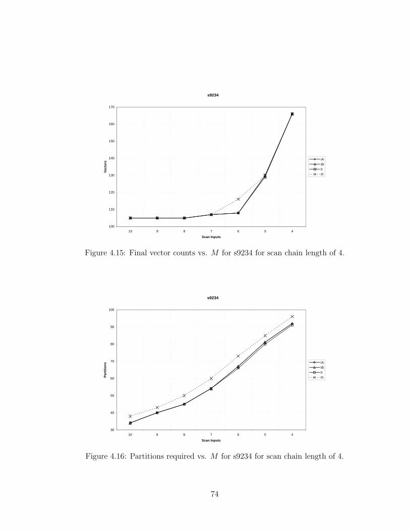
s9234

100

110

120

130

140

150

160

170

10 9 8 7 6 5 4

Scan Inputs

Vec

tors

IA

IB

II

III

Figure 4.15: Final vector counts vs. M for s9234 for scan chain length of 4.

s9234

30

40

50

60

70

80

90

100

10 9 8 7 6 5 4

Scan Inputs

Par

titi

on

s IA

IB

II

III

Figure 4.16: Partitions required vs. M for s9234 for scan chain length of 4.

74

s13207

80.00%

82.00%

84.00%

86.00%

88.00%

90.00%

92.00%

94.00%

96.00%

98.00%

19 11 10 9 8 7 6 5 4 3

Scan Inputs

Co

mp

ress

ion

Rat

io

IA

IB

II

III

Figure 4.17: Overall compression vs. M for s13207 for scan chain length of 7.

s13207

230

235

240

245

250

255

260

265

270

19 11 10 9 8 7 6 5 4 3

Scan Inputs

Vec

tors

IA

IB

II

III

Figure 4.18: Final vector counts vs. M for s13207 for scan chain length of 7.

75

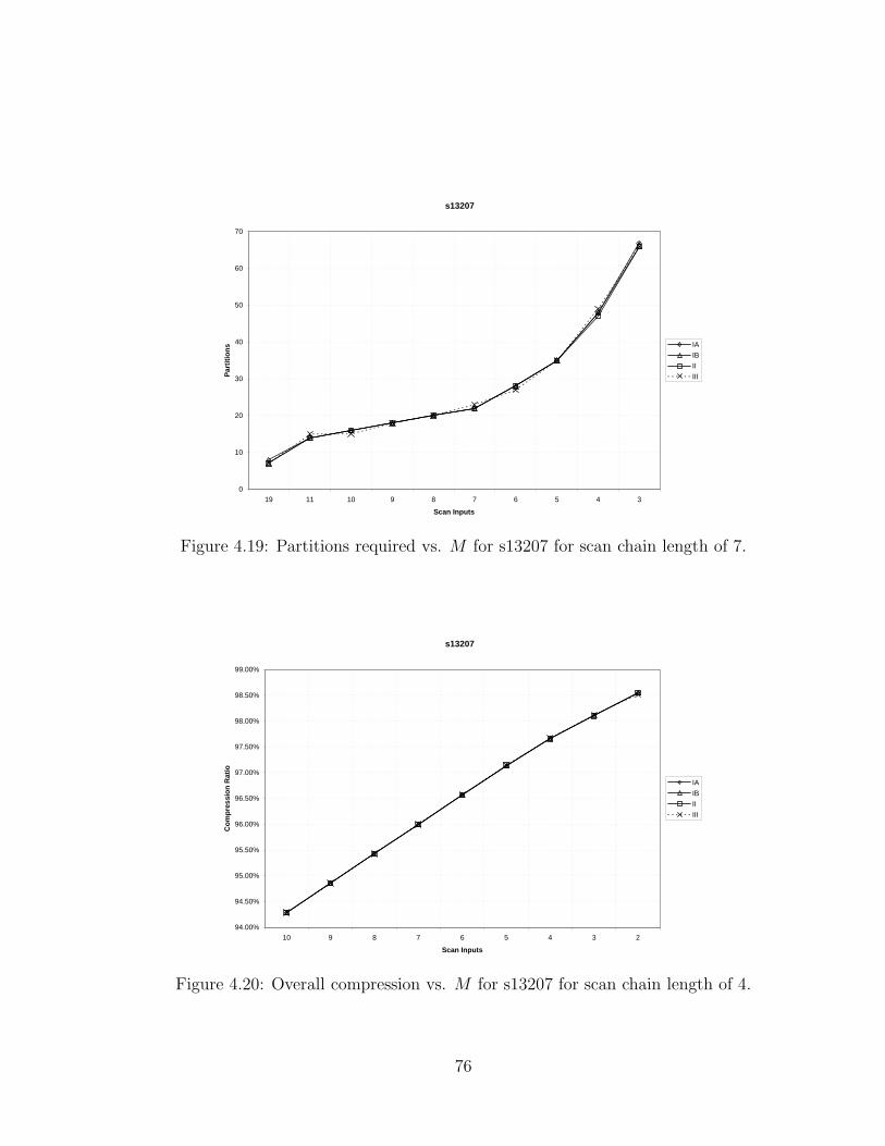
s13207

0

10

20

30

40

50

60

70

19 11 10 9 8 7 6 5 4 3

Scan Inputs

Par

titi

on

s IA

IB

II

III

Figure 4.19: Partitions required vs. M for s13207 for scan chain length of 7.

s13207

94.00%

94.50%

95.00%

95.50%

96.00%

96.50%

97.00%

97.50%

98.00%

98.50%

99.00%

10 9 8 7 6 5 4 3 2

Scan Inputs

Co

mp

ress

ion

Rat

io

IA

IB

II

III

Figure 4.20: Overall compression vs. M for s13207 for scan chain length of 4.

76

s13207

220

230

240

250

260

270

280

290

300

310

10 9 8 7 6 5 4 3 2

Scan Inputs

Vec

tors

IA

IB

II

III

Figure 4.21: Final vector counts vs. M for s13207 for scan chain length of 4.

s13207

10

30

50

70

90

110

130

150

170

10 9 8 7 6 5 4 3 2

Scan Inputs

Par

titi

on

s IA

IB

II

III

Figure 4.22: Partitions required vs. M for s13207 for scan chain length of 7.

77

s15850

80.00%

82.00%

84.00%

86.00%

88.00%

90.00%

92.00%

94.00%

16 15 14 13 12 11 10 9 8 7 6 5 4 3

Scan Inputs

Co

mp

ress

ion

Rat

io

IA

IB

II

III

Figure 4.23: Overall compression vs. M for s15850 for scan chain length of 7.

s15850

90

110

130

150

170

190

16 15 14 13 12 11 10 9 8 7 6 5 4 3

Scan Inputs

Vec

tors

IA

IB

II

III

Figure 4.24: Final vector counts vs. M for s15850 for scan chain length of 7.

78

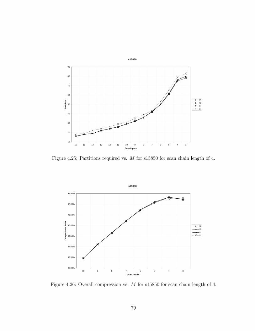
s15850

10

20

30

40

50

60

70

80

90

16 15 14 13 12 11 10 9 8 7 6 5 4 3

Scan Inputs

Par

titi

on

s IA

IB

II

III

Figure 4.25: Partitions required vs. M for s15850 for scan chain length of 4.

s15850

93.00%

93.50%

94.00%

94.50%

95.00%

95.50%

96.00%

96.50%

10 9 8 7 6 5 4 3

Scan Inputs

Co

mp

ress

ion

Rat

io

IA

IB

II

III

Figure 4.26: Overall compression vs. M for s15850 for scan chain length of 4.

79

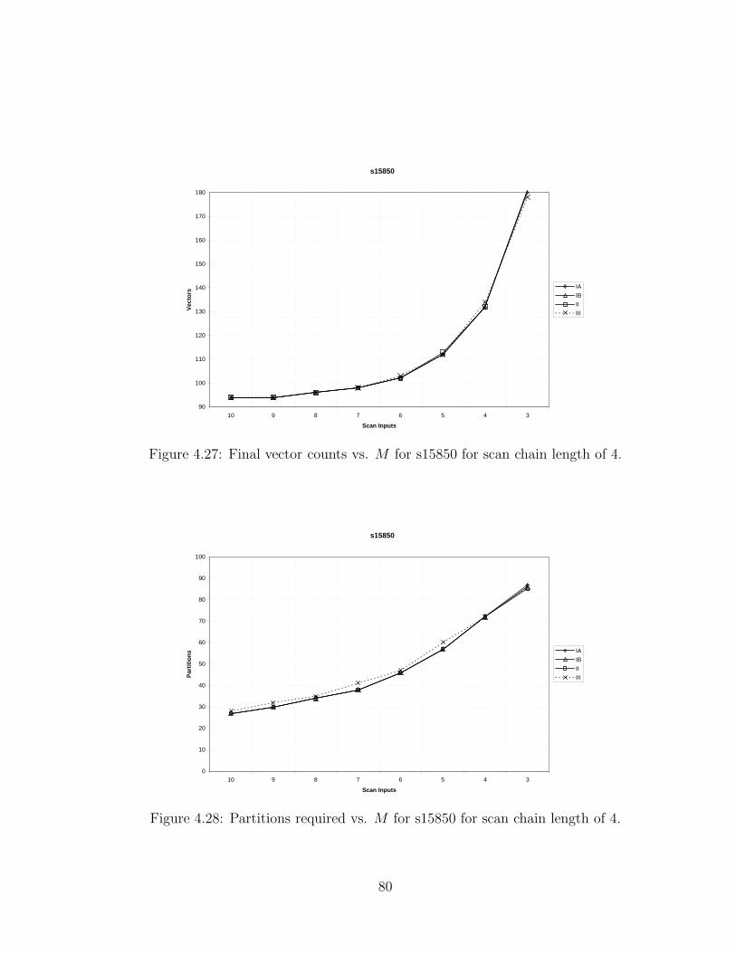
s15850

90

100

110

120

130

140

150

160

170

180

10 9 8 7 6 5 4 3

Scan Inputs

Vec

tors

IA

IB

II

III

Figure 4.27: Final vector counts vs. M for s15850 for scan chain length of 4.

s15850

0

10

20

30

40

50

60

70

80

90

100

10 9 8 7 6 5 4 3

Scan Inputs

Par

titi

on

s IA

IB

II

III

Figure 4.28: Partitions required vs. M for s15850 for scan chain length of 4.

80

s35932

0.00%

10.00%

20.00%

30.00%

40.00%

50.00%

60.00%

70.00%

80.00%

73 68 67 66 65 64 63 62 59 55 54 38 33 22 18 17 16 15 14 13 12 11 10

Scan Inputs

Co

mp

ress

ion

Rat

io

IA

IB

II

III

Figure 4.29: Overall compression vs. M for s35932 for scan chain length of 18.

s35932

10

15

20

25

30

35

40

45

73 68 67 66 65 64 63 62 59 55 54 38 33 22 18 17 16 15 14 13 12 11 10

Scan Inputs

Vec

tors

IA

IB

II

III

Figure 4.30: Final vector counts vs. M for s35932 for scan chain length of 18.

81

s35932

0

2

4

6

8

10

12

14

16

18

20

22

24

26

73 68 67 66 65 64 63 62 59 55 54 38 33 22 18 17 16 15 14 13 12 11 10

Scan Inputs

Par

titi

on

s IA

IB

II

III

Figure 4.31: Partitions required vs. M for s35932 for scan chain length of 18.

s35932

70.00%

72.00%

74.00%

76.00%

78.00%

80.00%

82.00%

84.00%

86.00%

88.00%

90.00%

27 25 23 22 21 19 17 15 13

Scan Inputs

Co

mp

ress

ion

Rat

io

IA

IB

II

III

Figure 4.32: Overall compression vs. M for s35932 for scan chain length of 9.

82

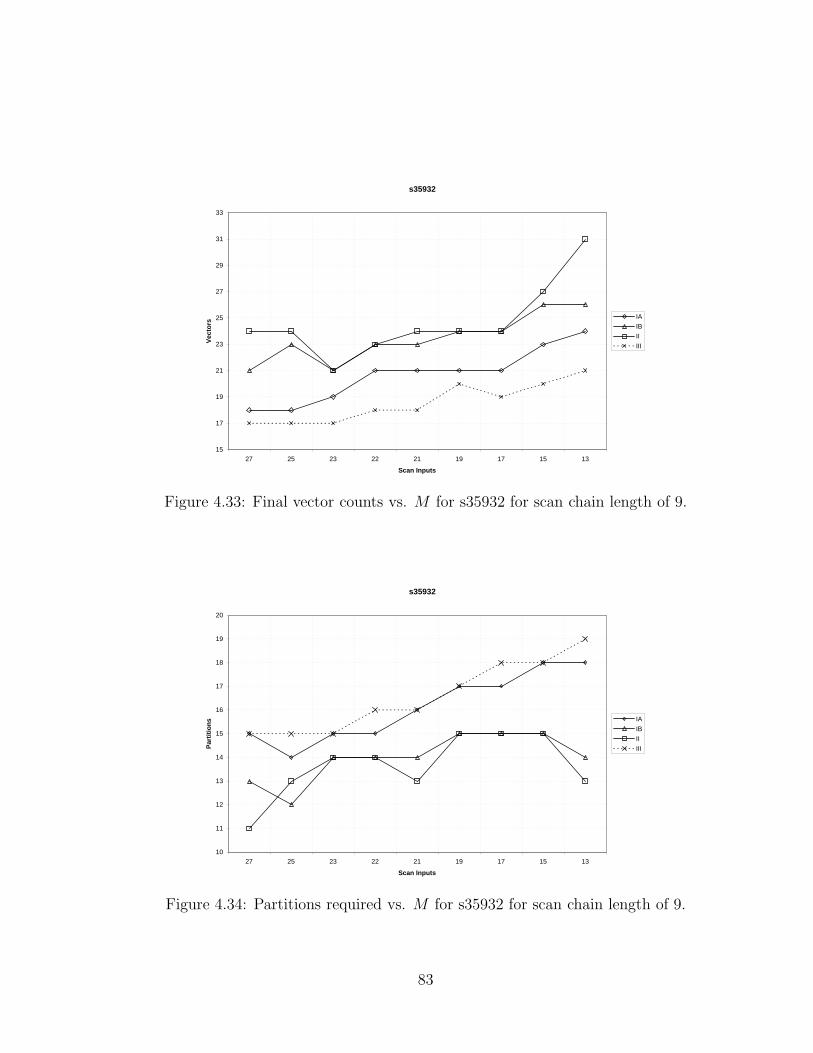
s35932

15

17

19

21

23

25

27

29

31

33

27 25 23 22 21 19 17 15 13

Scan Inputs

Vec

tors

IA

IB

II

III

Figure 4.33: Final vector counts vs. M for s35932 for scan chain length of 9.

s35932

10

11

12

13

14

15

16

17

18

19

20

27 25 23 22 21 19 17 15 13

Scan Inputs

Par

titi

on

s IA

IB

II

III

Figure 4.34: Partitions required vs. M for s35932 for scan chain length of 9.

83

s38417

67.00%

68.00%

69.00%

70.00%

71.00%

72.00%

73.00%

74.00%

75.00%

32 30 28 26 24 22 20 18 16 15

Scan Inputs

Co

mp

ress

ion

Rat

io

IA

IB

II

III

Figure 4.35: Overall compression vs. M for s38417 for scan chain length of 17.

s38417

60

70

80

90

100

110

120

130

32 30 28 26 24 22 20 18 16 15

Scan Inputs

Vec

tors

IA

IB

II

III

Figure 4.36: Final vector counts vs. M for s38417 for scan chain length of 17.

84

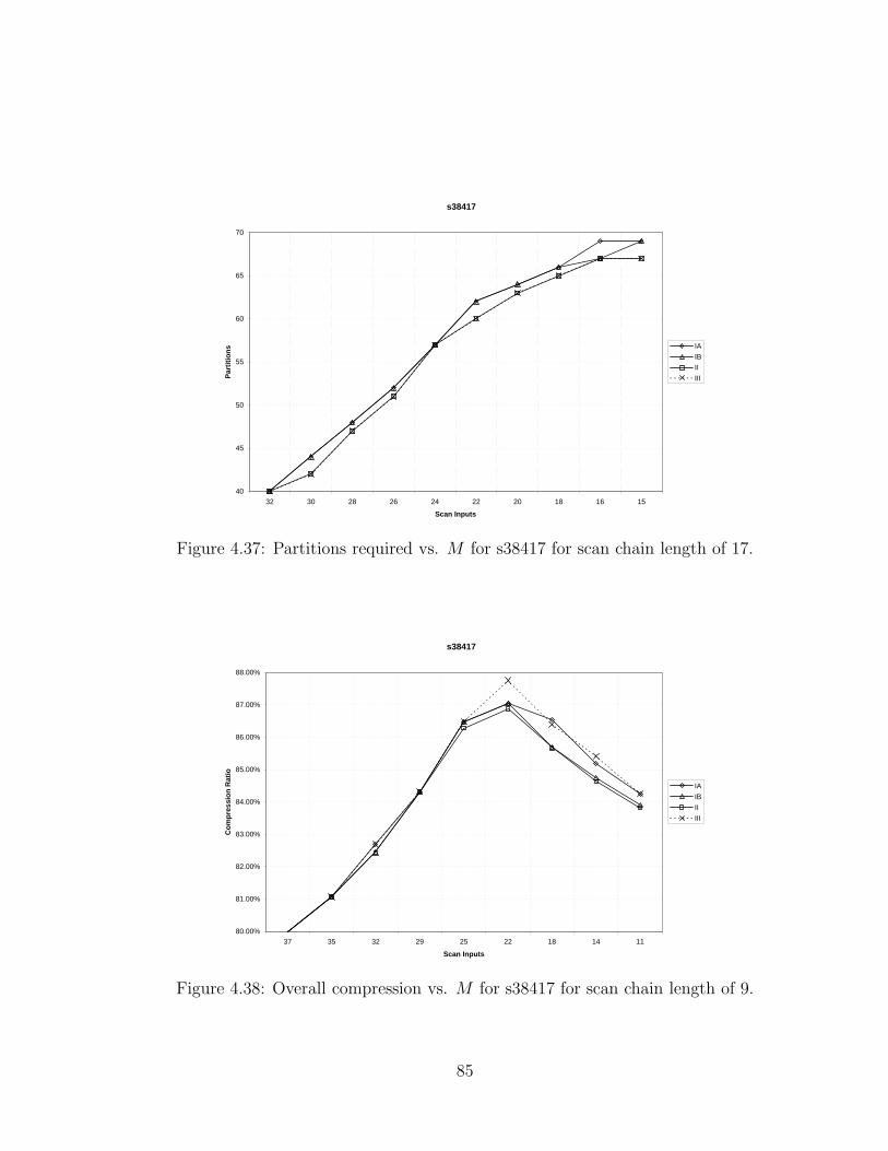
s38417

40

45

50

55

60

65

70

32 30 28 26 24 22 20 18 16 15

Scan Inputs

Par

titi

on

s IA

IB

II

III

Figure 4.37: Partitions required vs. M for s38417 for scan chain length of 17.

s38417

80.00%

81.00%

82.00%

83.00%

84.00%

85.00%

86.00%

87.00%

88.00%

37 35 32 29 25 22 18 14 11

Scan Inputs

Co

mp

ress

ion

Rat

io

IA

IB

II

III

Figure 4.38: Overall compression vs. M for s38417 for scan chain length of 9.

85

s38417

60

80

100

120

140

160

180

200

37 35 32 29 25 22 18 14 11

Scan Inputs

Vec

tors

IA

IB

II

III

Figure 4.39: Final vector counts vs. M for s38417 for scan chain length of 9.

s38417

30

35

40

45

50

55

60

65

70

75

37 35 32 29 25 22 18 14 11

Scan Inputs

Par

titi

on

s IA

IB

II

III

Figure 4.40: Partitions required vs. M for s38417 for scan chain length of 9.

86

s38584

40.00%

45.00%

50.00%

55.00%

60.00%

65.00%

70.00%

75.00%

80.00%

85.00%

90.00%

56 51 41 39 25 19 17 15 12 10

Scan Inputs

Co

mp

ress

ion

Rat

io

IA

IB

II

III

Figure 4.41: Overall compression vs. M for s38584 for scan chain length of 15.

s38584

110

111

112

113

114

115

116

117

118

119

120

56 51 41 39 25 19 17 15 12 10

Scan Inputs

Vec

tors

IA

IB

II

III

Figure 4.42: Final vector counts vs. M for s38584 for scan chain length of 15.

87

s38584

10

20

30

40

50

60

70

56 51 41 39 25 19 17 15 12 10

Scan Inputs

Par

titi

on

s IA

IB

II

III

Figure 4.43: Partitions required vs. M for s38584 for scan chain length of 15.

s38584

80.00%

82.00%

84.00%

86.00%

88.00%

90.00%

92.00%

94.00%

96.00%

98.00%

35 32 29 21 14 10 8 6 4

Scan Inputs

Co

mp

ress

ion

Rat

io

IA

IB

II

III

Figure 4.44: Overall compression vs. M for s38584 for scan chain length of 8.

88

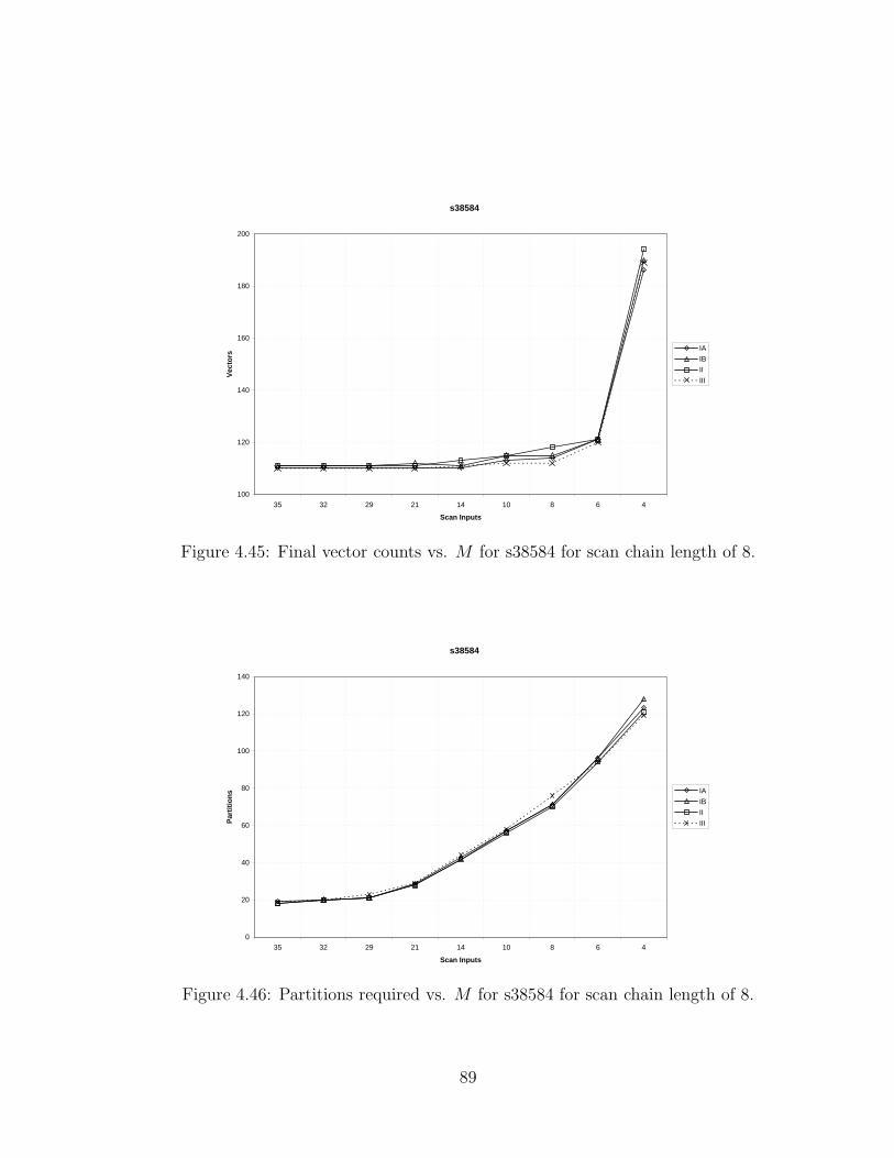
s38584

100

120

140

160

180

200

35 32 29 21 14 10 8 6 4

Scan Inputs

Vec

tors

IA

IB

II

III

Figure 4.45: Final vector counts vs. M for s38584 for scan chain length of 8.

s38584

0

20

40

60

80

100

120

140

35 32 29 21 14 10 8 6 4

Scan Inputs

Par

titi

on

s IA

IB

II

III

Figure 4.46: Partitions required vs. M for s38584 for scan chain length of 8.

89

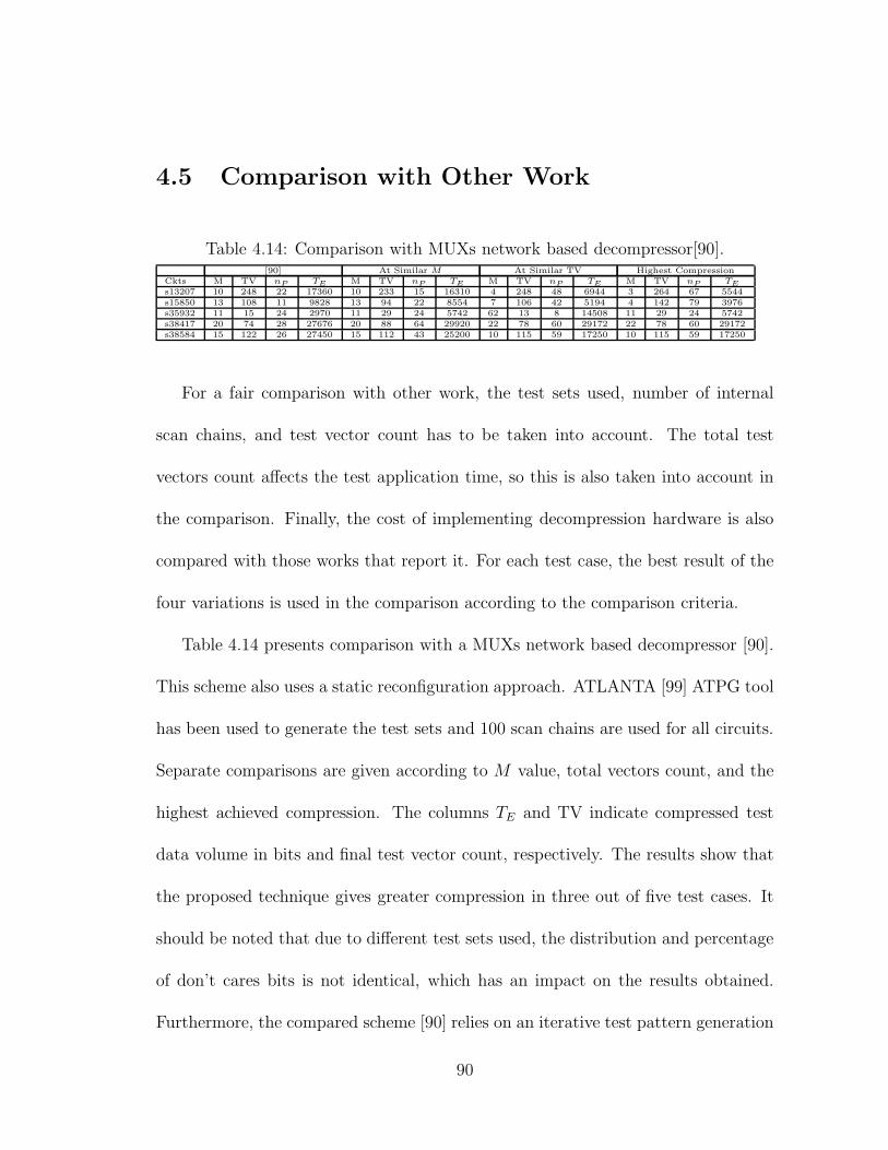
4.5 Comparison with Other Work

Table 4.14: Comparison with MUXs network based decompressor[90].[90] At Similar M At Similar TV Highest Compression

Ckts M TV nP TE M TV nP TE M TV nP TE M TV nP TE

s13207 10 248 22 17360 10 233 15 16310 4 248 48 6944 3 264 67 5544s15850 13 108 11 9828 13 94 22 8554 7 106 42 5194 4 142 79 3976s35932 11 15 24 2970 11 29 24 5742 62 13 8 14508 11 29 24 5742s38417 20 74 28 27676 20 88 64 29920 22 78 60 29172 22 78 60 29172s38584 15 122 26 27450 15 112 43 25200 10 115 59 17250 10 115 59 17250

For a fair comparison with other work, the test sets used, number of internal

scan chains, and test vector count has to be taken into account. The total test

vectors count affects the test application time, so this is also taken into account in

the comparison. Finally, the cost of implementing decompression hardware is also

compared with those works that report it. For each test case, the best result of the

four variations is used in the comparison according to the comparison criteria.

Table 4.14 presents comparison with a MUXs network based decompressor [90].

This scheme also uses a static reconfiguration approach. ATLANTA [99] ATPG tool

has been used to generate the test sets and 100 scan chains are used for all circuits.

Separate comparisons are given according to M value, total vectors count, and the

highest achieved compression. The columns TE and TV indicate compressed test

data volume in bits and final test vector count, respectively. The results show that

the proposed technique gives greater compression in three out of five test cases. It

should be noted that due to different test sets used, the distribution and percentage

of don’t cares bits is not identical, which has an impact on the results obtained.

Furthermore, the compared scheme [90] relies on an iterative test pattern generation

90

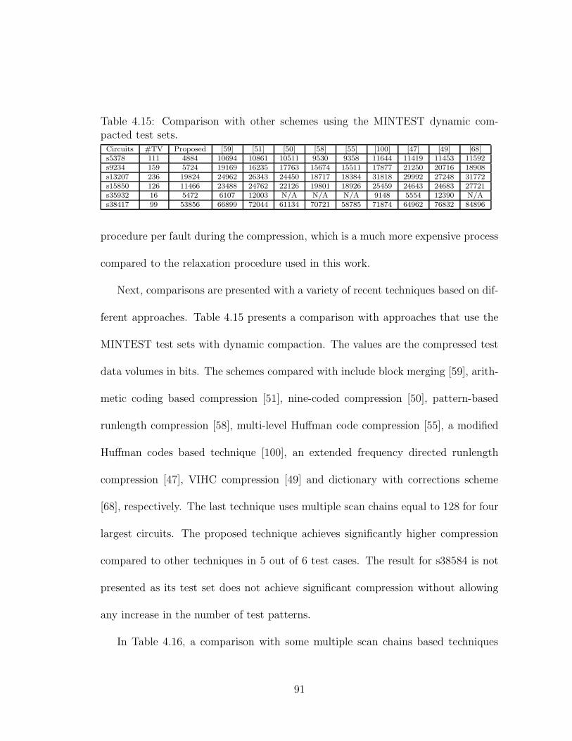
Table 4.15: Comparison with other schemes using the MINTEST dynamic com-pacted test sets.

Circuits #TV Proposed [59] [51] [50] [58] [55] [100] [47] [49] [68]s5378 111 4884 10694 10861 10511 9530 9358 11644 11419 11453 11592s9234 159 5724 19169 16235 17763 15674 15511 17877 21250 20716 18908s13207 236 19824 24962 26343 24450 18717 18384 31818 29992 27248 31772s15850 126 11466 23488 24762 22126 19801 18926 25459 24643 24683 27721s35932 16 5472 6107 12003 N/A N/A N/A 9148 5554 12390 N/As38417 99 53856 66899 72044 61134 70721 58785 71874 64962 76832 84896

procedure per fault during the compression, which is a much more expensive process

compared to the relaxation procedure used in this work.

Next, comparisons are presented with a variety of recent techniques based on dif-

ferent approaches. Table 4.15 presents a comparison with approaches that use the

MINTEST test sets with dynamic compaction. The values are the compressed test

data volumes in bits. The schemes compared with include block merging [59], arith-

metic coding based compression [51], nine-coded compression [50], pattern-based

runlength compression [58], multi-level Huffman code compression [55], a modified

Huffman codes based technique [100], an extended frequency directed runlength

compression [47], VIHC compression [49] and dictionary with corrections scheme

[68], respectively. The last technique uses multiple scan chains equal to 128 for four

largest circuits. The proposed technique achieves significantly higher compression

compared to other techniques in 5 out of 6 test cases. The result for s38584 is not

presented as its test set does not achieve significant compression without allowing

any increase in the number of test patterns.

In Table 4.16, a comparison with some multiple scan chains based techniques

91

is given. Results for the proposed scheme are given with and without test vector

increase over the MINTEST static compacted test set. For the smallest two circuits

near 64 scan chains are used while for the larger five circuits both near 100 and

200 scan chains are used. The scan chains and test sets used in other schemes

are as follows: Shi et al. [88] use a commercial ATPG tool and compression is

reported with 200 scan chains, Rao et al. [81] use ATLANTA ATPG tool [99] and

compression is reported for scan chain lengths of 2, Li et al. [92] use 64 and 200

scan chains respectively for the smallest two and larger five circuits with MINTEST

test sets without compaction, Hayashi et al. [60] use X-maximal program for test

set generation with scan chains lengths varying between 16 and 64 in powers of 2,

and Tang et al. [101] do not specify the specifics of test sets and all results are

reported with 256 scan chains except for s15850, where 128 are used. The proposed

technique achieves higher compression with most of the test cases at comparable or

much lower vector counts except for s35932, due to the reasons mentioned before.

92

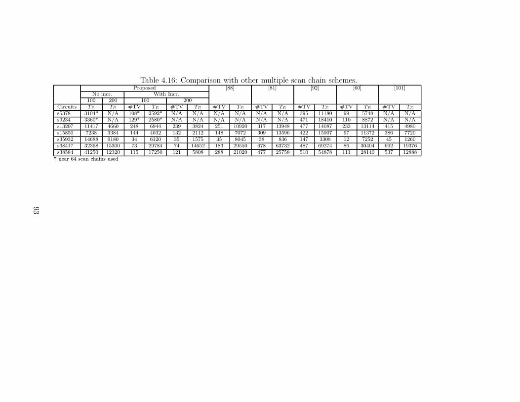
Table 4.16: Comparison with other multiple scan chain schemes.Proposed [88] [81] [92] [60] [101]

No incr. With Incr.100 200 100 200

Circuits TE TE #TV TE #TV TE #TV TE #TV TE #TV TE #TV TE #TV TE

s5378 3104* N/A 108* 2592* N/A N/A N/A N/A N/A N/A 395 11180 99 5748 N/A N/As9234 3360* N/A 129* 2580* N/A N/A N/A N/A N/A N/A 471 18410 110 8872 N/A N/As13207 11417 4660 248 6944 239 3824 251 10920 317 13948 477 14087 233 13114 415 4980s15850 7238 3384 144 4032 132 2112 148 7072 309 13596 422 15907 97 11372 386 7720s35932 14688 9180 34 6120 35 1575 35 8045 38 836 147 3308 12 7252 45 1260s38417 32368 15300 73 29784 74 14652 183 29550 678 63732 487 69274 86 30404 692 19376s38584 41250 12320 115 17250 121 5808 288 21020 477 25758 510 54878 111 28140 537 12888

* near 64 scan chains used

93

4.6 Hardware Cost Comparison

Table 4.17: Comparison of H/W costs with two multiple scan chains schemes.

Proposed [66] [93]No TV increment With TV Increment

Circuit H/W TE H/W TE H/W TE H/W TE

s5378 1536 3104 1518 2592 2636 6124 628 11180

s9234 2225 3360 2717 2592 3701 11388 1397 18410

s13207 1711 11417 2228 5544 4293 6093 1270 14087

s15850 2120 7238 3178 3976 3908 12947 1469 15907

s35932 987 14688 1388 5742 3026 1040 36 3308

s38417 4172 32368 4787 29172 2382 58397 74 69274

s38584 2717 41250 4559 17250 5036 52612 1320 54878

Unlike compression results, extensive comparison of hardware cost with previous

work is not always possible because either the actual hardware cost and the specific

implementation library is not reported, or, the schemes are based on a single scan

chain. To compare hardware cost, two schemes based on multiple scan chains are

considered that report hardware cost using the lsi 10k library provided with the

Synopsys Design Compiler. Of these, one is a dictionary based scheme [66] while

the other uses width compression along with dictionary compression [93]. Table

4.17 reports the hardware cost obtained with proposed algorithms for each test case

for two compression values. These two results correspond to compression obtained

with and without increment in test vector counts using near 100 scan chains. Since

the hardware cost is dependent upon partitioning, these values give a an idea about

the difference in hardware cost for different compression values. It is observed that

94

compared to the dictionary scheme [66], much greater compressions are obtained

at lower or similar hardware costs. In case of the other work [92], the reported

hardware costs are smaller but compression is significantly lesser compared to the

proposed scheme in all test cases except s35932.

95

Chapter 5

Conclusions and Future Work

An effective test vector compression technique has been proposed in this work that

uses test set partitioning and bottleneck test vector decomposition through relax-

ation. The technique targets a user specified number of ATE channels to achieve

test data compression and it can explore tradeoffs among compression ratio, area

overhead and test vectors count. Instead of ATPG, the technique relies on a fast

test relaxation algorithm and can work with compacted test sets to achieve high

compression with much lower vector counts, thus minimizing test application time.

The results clearly show that the proposed technique achieves significantly greater

test volume reduction compared to other recent work.

The proposed multiple scan chain compression technique can take advantage of

test vector relaxation that allows obtaining don’t cares on specified bit positions in

a scan vector. The test vector relaxation used in this work for obtaining atomic

96

test vectors gives equal weight to all bit positions in a given input test vector when

identifying don’t cares. However, this algorithm can be modified so that it prioritizes

certain bit positions in the vector so that these positions are given preference over

other candidate positions when obtaining don’t cares.

In order to understand how this enhancement can benefit the proposed tech-

nique, recall that the actual compression is determined by the colors needed by the

bottleneck vectors, which depends on both the percentage of specified bits present

in the test vector and their relative positions. The incremental fault dropping used

in the proposed technique indirectly minimizes the number of specified bits when

obtaining new vector(s) from the original bottleneck vector. However, no attempt

is made to obtain don’t cares at specific bit positions. It is observed that a single

value conflict in a bit position can lead to higher than desired number of colors.

By identifying the positions that must have don’t cares after relaxation and guiding

the relaxation process, improved compression can be obtained as less colors will be

needed, and/or the amount of decomposition necessary for each bottleneck vector

may be reduced.

Besides improving the compression ratio, controlled relaxation can also improve

the partitioning results. Following the same reasoning as before, if a vector doesn’t fit

in a given partition, conflicting positions may be identified and a different relaxation

can be attempted to make the vector fit in.

It should be noted that there is no guaranteed possibility that an alternate

97

relaxation will always lead to an improved result. However, the idea is intuitive

enough to be worth experimenting and empirical results will decide the actual benefit

of this enhancement to the existing technique.

98

APPENDIX

Color Histograms

The color histograms of all MINTEST generated test cases using static com-

paction, for the specified scan chain lengths, are given in Figures A.1 - A.12.

99

s5378 Color Histogram

1

12

17

21

23

5

12

3

1 1 1

0

5

10

15

20

25

3 4 5 6 7 8 9 10 11 12 13

Colors

#Vec

tors

Figure A.1: Color histogram of vectors in s5378 test set with scan chain length of 4.

s9234 Color Histogram

4

6

25

33

24

5 5

1 1 1

0

5

10

15

20

25

30

35

2 3 4 5 6 7 8 9 10 11

Colors

#Vec

tors

Figure A.2: Color histogram of vectors in s9234 test set with scan chain length of 4.

100

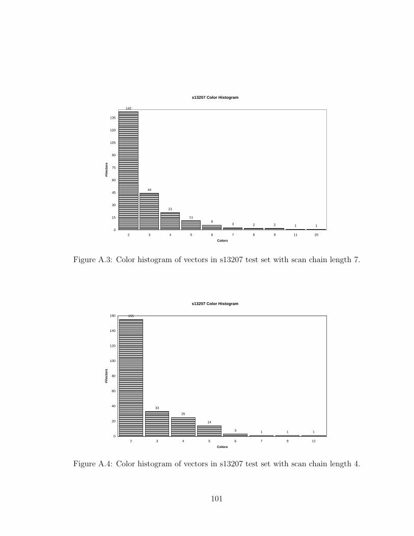
s13207 Color Histogram

142

44

21

116

3 2 2 1 10

15

30

45

60

75

90

105

120

135

2 3 4 5 6 7 8 9 11 20

Colors

#Vec

tors

Figure A.3: Color histogram of vectors in s13207 test set with scan chain length 7.

s13207 Color Histogram

155

33

25

14

3 1 1 10

20

40

60

80

100

120

140

160

2 3 4 5 6 7 9 12

Colors

#Vec

tors

Figure A.4: Color histogram of vectors in s13207 test set with scan chain length 4.

101

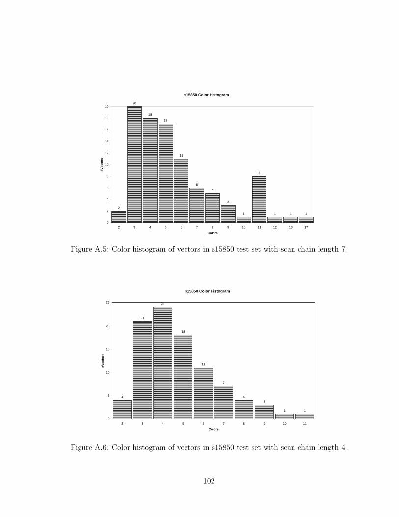
s15850 Color Histogram

2

20

18

17

11

6

5

3

1

8

1 1 1

0

2

4

6

8

10

12

14

16

18

20

2 3 4 5 6 7 8 9 10 11 12 13 17

Colors

#Vec

tors

Figure A.5: Color histogram of vectors in s15850 test set with scan chain length 7.

s15850 Color Histogram

4

21

24

18

11

7

43

1 1

0

5

10

15

20

25

2 3 4 5 6 7 8 9 10 11

Colors

#Vec

tors

Figure A.6: Color histogram of vectors in s15850 test set with scan chain length 4.

102

s35932 Color Histogram

1 1 1 1 1 1 1 1 1 1 1 1

0

1

2

13 15 22 33 38 54 55 59 62 63 68 73

Colors

#Vec

tors

Figure A.7: Color histogram of vectors in s35932 test set with scan chain length 18.

s35932 Color Histogram

1 1 1 1 1 1 1 1

2

1 1

0

1

2

17 19 27 33 35 54 55 59 75 85 91

Colors

#Vec

tors

Figure A.8: Color histogram of vectors in s35932 test set with scan chain length 9.

103

s38417 Color Histogram

2

1

2 2

1

4

9

1

4

5

7

3

4

5

2

5

2

1 1

2 2

1 1 1

0

1

2

3

4

5

6

7

8

9

10

11 14 15 16 17 18 19 20 21 22 23 24 25 26 27 28 29 31 32 33 40 42 43 65

Colors

#Vec

tors

Figure A.9: Color histogram of vectors in s38417 test set with scan chain length 17.

s38417 Color Histogram

1 1 1 1

2

4

5

4

6

5

10

9

4

3

2

1 1

2

1

2

1 1 1

0

1

2

3

4

5

6

7

8

9

10

11 12 14 15 16 17 18 19 20 21 22 23 24 25 26 27 28 29 31 32 35 37 61

Colors

#Vec

tors

Figure A.10: Color histogram of vectors in s38417 test set with scan chain length 9.

104

s38584 Color Histogram

12

12

21

30

14

4

1

3

1

43

1 12

1 1 1 1 12

1 1 1

0

5

10

15

20

25

30

3 4 5 6 7 8 9 10 11 12 13 14 15 17 18 21 23 25 34 39 40 41 51 56

Colors

#Vec

tors

Figure A.11: Color histogram of vectors in the s38584 set with scan chain length 15.

s38584 Color Histogram

1

5

17

40

18

2

6

23 3

21

21 1 1 1 1 1 1 1

0

5

10

15

20

25

30

35

40

3 4 5 6 7 8 9 10 11 12 13 14 18 21 26 28 29 31 32 35 46

Colors

#Vec

tors

Figure A.12: Color histogram of vectors in s38584 test set with scan chain length 8.

105

Bibliography

[1] Jack Horgan. TEST & ATE - Cost of Test. EDA Cafe Weekly,

http://www.edacafe.com, March 2004.

[2] Kirk Brisacher, Rohit Kapur, and Steve Smith. The History and Future of

Scan Design. EETimes Online, http://www.eetimes.com, September 2005.

[3] Rohit Kapur and Kirk Brisacher. Next Generation Scan Synthesis. Synop-

sys.com Compiler, May 2005.

[4] Harald Vranken, Friedrich Hapke, Soenke Rogge, Domenico Chindamo, and

Erik H. Volkerink. ATPG padding and ATE Vector repeat per port for Re-

ducing Test Data Volume. In ITC ’03: Proceedings of the International Test

Conference, page 1069, Washington, DC, USA, 2003. IEEE Computer Society.

[5] Takahiro J. Yamaguchi, Dong Sam Ha, Masahiro Ishida, and Tadahiro Ohmi.

A Method for Compressing Test Data Based on Burrows-Wheeler Transfor-

mation. IEEE Trans. Comput., 51(5):486–497, 2002.

106

[6] International Technology Roadmap for Semiconductors,

http://public.itrs.net/files/1999 sia roadmap/home.htm. 1999.

[7] Brian T. Murray and J.P. Hayes. Testing ICs: Getting to the Core of the

Problem. IEEE Computer Magazine, 29(11):32–38, November 1996.

[8] Anshuman Chandra and Krishnendu Chakrabarty. Test Resource Partition-

ing for SOCs. IEEE Design & Test of Computers, pages 80–91, September-

October 2001.

[9] T. Hiraide, K. O. Boateng, H. Konishi, K. Itaya, M. Emori, and H. Yamanaka.

BIST-Aided Scan Test-A New Method for Test Cost Reduction. pages 359–

364. VLSI Test Symposium, April 2003.

[10] C. Chen and S. K. Gupta. Efficient BIST TPG Design and Test Set Com-

paction via Input Reduction. IEEE Trans. Computer-Aided Design Integr.

Circuits Syst., 17(8):692 –705, August 1998.

[11] Aiman El-Maleh and Ali Al-Suwaiyan. An Efficient Test Relaxation Technique

for Combinational & Full-Scan Sequential Circuits. In VTS ’02: Proceedings

of the 20th IEEE VLSI Test Symposium, page 53, Washington, DC, USA,

2002. IEEE Computer Society.

[12] Tom Lecklider. Test Pattern Compression Saves

Time and Bits. EE’05: Evaluation Engineering,

107

http://www.evaluationengineering.com/archive/articles/0705/0705test pattern.asp,

July 2005.

[13] M. Lange. Adopting the Right Embedded Com-

pression Solution. EE-Evaluation Engineering,

www.evaluationengineering.com/archive/articles/0505

/0505adopting right.asp, pages 32–40, May 2005.

[14] D. Hochbaum. An optimal test compression procedure for combinational cir-

cuits. Tran. on Computer-Aided Design of Integrated Circuits and Systems,

15(10):1294–1299, October 1996.

[15] Aiman El-Maleh and Yahya E. Osais. Test Vector Decomposition-Based Static

Compaction Algorithms for Combinational Circuits. ACM Transactions on

Design Automation of Electronic Systems, 8(4):430–459, October 2003.

[16] Julien Dalmasso, Marie-Lise Flottes, and Bruno Rouzeyre. Fitting ATE Chan-

nels With Scan Chains: A Comparison Between a Test Data Compression

Technique and Serial Loading of Scan Chains. In DELTA06: Proceedings of

the Third IEEE International Workshop on Electronic Design, Test and Ap-

plications, 2006.

[17] K. J. Lee, Ji-Jan Chen, and C. H. Huang. Broadcasting Test Patterns to

Multiple Circuits. IEEE Trans. Computer-Aided Design Integr. Circuits Syst.,

108

18(12):1793–1802, December 1999.

[18] Ilker Hamzaoglu and Janak H. Patel. Reducing Test Application Time for

Full Scan Embedded Cores. pages 260–267. FTC’99: IEEE International

Symposium on Fault Tolerant Computing, 1999.

[19] T. C. Huang and K. J. Lee. A Token Scan Architecture for Low Power Testing.

pages 660–669. ITC’01: International Test Conference, October 2001.

[20] S. Sharifi, M. Hosseinabadi, P. Riahi, and Zainalabedin Navabi. Reducing

Test Power, Time and Data Volume in soc Testing Using Selective trigger

Scan Architecture. DFT’03: International Symposium on Defect and Fault

Tolerance, 2003.

[21] Ozgur Sinanoglu and Alex Orailoglu. A Novel Scan Architecture for Power-

Efficient Rapid Test. pages 299–303. ICCAD’02: International Conference on

Computer-Aided Design, November 2002.

[22] S. Samaranayake, E. Gizdarski, N. Sitchinava, F. Neuveux, Rohit Kapur, and

T. Williams. A reconfigurable Shared Scan-in Architecture. In VTS’03: Pro-

ceedings of the 21st IEEE VLSI Test Symposium, April 2003.

[23] Dong Xiang, Jia-Guang Sun, Ming jing Chen, and S. Gu. Cost-Effective Scan

Architecture and a Test Application Scheme for Scan Testing with nonscan

109

Test Power and Test Application cost. US Patent Application 20040153978,

August 2004.

[24] A. Arslan and Alex Orailoglu. Circularscan: A Scan Architecture for Test

cost Reduction. pages 1290–1295. DATE04: Proceedings of the Design, Au-

tomation and Test in Europe Conference and Exhibition, February 2004.

[25] Ahmad Al-Yamani, Erik Chmelar, and Mikhail Grinchuck. Segmented Ad-

dressable Scan Architecture. Proc. VLSI Test Symposium (VTS05), 2005.

[26] P. Rosinger, B.M. Al-Hashimi, and N. Nicolici. Scan architecture with mutu-

ally exclusive scan segment activation for shift and capture-power reduction.

IEEE Transactions on Computer-Aided Design, 23(7):1142–1153, July 2004.

[27] H. Ando. Testing VLSI with Random Access Scan. In Proc. Of the COMP-

CON, pages 50–52, 1980.

[28] T. Williams and R. Mercer. Design for Testability-A Survery. IEEE Trans.

On Computers, C-31(1):2–15, January 1982.

[29] D. Baik, Seiji Kajihara, and Kewal K. Saluja. Random Access Scan: A solution

to Test Power, Test Data Volume and Test Time. In VLSID04: International

Conference on VLSI Design, pages 883–888, 2004.

110

[30] Baris Arslan and Alex Orailoglu. Test cost Reduction Through a reconfig-

urable Scan Architecture. In ITC International Test Conference, pages 945–

952, 2004.

[31] Anand S. Mudlapur, Vishwani D. Agrawal, and Adit D. Singh. A Novel

Random Access Scan Flip-Flop Design. In 9th VLSI Design and Test Symp,

pages 11–13, 2005.

[32] Anand S. Mudlapur, Vishwani D. Agrawal, and Adit D. Singh. A Random

Access Scan Architecture to Reduce Hardware Overhead. In Intl. Test Conf.,

2005.

[33] Dong Hyun Baik and Kewal K. Saluja. Progressive Random Access Scan: A

Simultaneous Solution to Test Power, Test Data Volume and Test Time. In

Intl. Test Conf., 2005.

[34] Dong Hyun Baik and Kewal K. Saluja. State-reuse Test Generation for Pro-

gressive Random Access Scan: Solution to Test Power, Application Time and

Data Size. In ATS 2005, 2005.

[35] Dong Hyun Baik and Kewal K. Saluja. Test Cost Reduction Using Parti-

tioned Grid Random Access Scan. In 19th International Conference on VLSI

Designm 2006, 2006.

111

[36] Laung-Terng Wang, Boryau Sheu, Zhigang Jiang, Zhigang Wang, and Shian-

ling Wu. PRAVS: Scan Compression on Random Access Scan. In Intl. Test

Conf., 2006.

[37] Shih Ping Lin, Chung Len Lee, and Jwu E Chen. A Cocktail Approach on

Random Access Scan Toward Low Power and High Efficiency Test. pages

94–99, 2005.

[38] Yu Hu, Yin-He Han, Xiao-Wei Li, Hua-Wei Li, and Xiao-Qing Wen. Com-

pression/Scan Co-Design for Reducing Test Data Volume, Scan-in Power Dis-

sipation and Test Application Time. 2005.

[39] V. Iyengar, Krishnendu Chakrabarty, and Brian T. Murray. Built-In Self

Testing of Sequential Circuits Using Precomputed Test Sets. pages 418–423.

VLSI Test Symposium, 1998.

[40] Abhijit Jas, J. Ghosh-Dastidar, and Nur A. Touba. Scan Vector Compres-

sion/Decompression Using Statistical Coding. pages 114–120. VLSI Test Sym-

posium, 1999.

[41] Abhijit Jas, J. Gosh-Dastidar, M. Ng, and Nur A. Touba. An Efficient Test

Vector Compression Scheme Using Selective Huffman Coding. IEEE Trans.

Computer-Aided Design Integr. Circuits Syst., 22(6):797–806, June 2003.

112

[42] Mehrdad Nourani and Mohammad Tehranipour. RL-Huffman Encoding for

Test Compression and Power Reduction in Scan Application. ACM Trans.

Design Automat. Electron. Syst., 10(1):91–115, January 2005.

[43] Anshuman Chandra and Krishnendu Chakrabarty. System-on-a-Chip Data

Compression and Decompression Architecture Based on Golomb Codes. IEEE

Trans. Computer-Aided Design Integr. Circuits Syst., 20(3):355–368, March

2001.

[44] Anshuman Chandra and Krishnendu Chakrabarty. Test Data Compres-

sion and Test Resource Partitioning for System-on-a-Chip Using Frequency-

directed Run-length (FDR) Codes. IEEE Trans. Comput., 52(8):1076–1088,

August 2003.

[45] Aiman El-Maleh, S. Al Zahir, and E. Khan. A Geometric-primitives-based

Compression Scheme for Testing System-on-Chip. pages 54–59. Proc. VLSI

Test Symp. (VTS’01), 2001.

[46] Anshuman Chandra and Krishnendu Chakrabarty. A Unified Approach to

Reduce SOC Test Data Volume, Scan Power, and Testing Time. IEEE Trans.

Computer-Aided Design Integr. Circuits Syst., 22(3):352–363, March 2003.

[47] Aiman El-Maleh and R. Al-Abaji. Extended Frequency-directed Run-length

Codes with Improved Application to System-on-a-Chip Test Data Compres-

113

sion. In ICECS’02: Int. Conf. on Electronic Circuits Systems, pages 449–452,

2002.

[48] P. Rosinger, Paul Theo Gonciari, Bashir M. Al-Hashimi, and Nicola Nicolici.

Simultaneous Reduction in Volume of Test Data and Power Dissipation for

System on-a-Chip. Electron. Lett., 37(24):1434–1436, 2001.

[49] Paul Theo Gonciari, Bashir M. Al-Hashimi, and Nicola Nicolici. Variable-

Length Input Huffman Coding for System-on-a-Chip Test. IEEE Trans.

Computer-Aided Design Integr. Circuits Syst., 22(6):783–796, June 2003.

[50] Mohammed Tehranipoor, Mehrdad Nourani, and Krishnendu Chakrabarty.

Nine-Coded Compression Technique for Testing Embedded Cores in SOCs.

IEEE Trans. Very Large Scale Integr. Syst., 13(6):719–731, June 2005.

[51] Hamidreza Hashempour and Fabrizio Lombardi. Application of Arithmetic

Coding to Compression. IEEE Trans. Comput., 54(9):1166–1177, September

2005.

[52] Sherief Reda and Alex Orailoglu. Reducing Test Application Time Through

Test Data Mutation Encoding. In DATE’02: Proceedings of the 2002 Design,

Automation and Test in Europe Conference and Exhibition, pages 1–7, 2002.

114

[53] A. Khoche, E.H. Volkerink, and S. Mitra. Packet-based Input Test Data

Compression Techniques. In In International Test Conference, page 154163,

2002.

[54] Sudhakar M. Reddy, Kohei Miyase, Seiji Kajihara, and Irith Pomeranz. On

Test Data Volume Reduction for Multiple Scan Chain designs. ACM Trans.

Des. Autom. Electron. Syst., 8(4):460–469, 2003.

[55] Xrysovalantis Kavousianos, Emmanouil Kalligeros, and Dimitris Nikolos. Effi-

cient Test-Data Compression for IP Cores Using Multilevel Huffman Coding.

In DATE ’06: Proceedings of the Conference on Design, Automation and Test

in Europe, pages 1033–1038, 3001 Leuven, Belgium, Belgium, 2006. European

Design and Automation Association.

[56] Ilia Polian, Alejandro Czutro, and Bernd Becker. Evolutionary Optimization

in Code-Based Test Compression. In DATE ’05: Proceedings of the Design,

Automation and Test in Europe Conference and Exhibition, 2005.

[57] Sunghoon Chun, YongJoon Kim, Jung-Been Im, and Sungho Kang. MICRO:

A New Hybrid Test Data Compression/Decompression Scheme. IEEE Trans-

actions on Very Large Scale Integration (VLSI) Systems, 14(6):649–654, June

2006.

115

[58] Xiaoyu Ruan and Rajendra Katti. An Efficient Data-Independent Technique

for Compressing Test Vectors in Systems-on-a-Chip. In ISVLSI ’06: Proceed-

ings of the IEEE Computer Society Annual Symposium on Emerging VLSI

Technologies and Architectures, page 153, Washington, DC, USA, 2006. IEEE

Computer Society.

[59] Aiman El-Maleh. An Efficient Test Vector Compression Technique Based on

Block Merging. In ISCAS ’06: Proceedings of the International Symposium

on Circuits and Systems, 2006.

[60] Terumine Hayashi, Haruna Yoshioka, Tsuyoshi Shinogi, Hidehiko Kita, and

Haruhiko Takase. Test Data Compression Technique Using Selective don’t-

care Identification. In ASP-DAC ’04: Proceedings of The 2004 Conference on

Asia South Pacific Design Automation, pages 230–233, Piscataway, NJ, USA,

2004. IEEE Press.

[61] Yasumi Doi, Seiji Kajihara, Xiaoqing Wen, Lei Li, and Krishnendu

Chakrabarty. Test Compression for Scan Circuits Using Scan Polarity Ad-

justment and Pinpoint Test Relaxation. In ASP-DAC ’05: Proceedings of

The 2005 Conference on Asia South Pacific Design Automation, pages 59–64,

New York, NY, USA, 2005. ACM Press.

[62] Sudhakar M. Reddy, Kohei Miyase, Seiji Kajihara, and Irith Pomeranz. On

Test Data Volume Reduction for Multiple Scan Chain Designs. page 103108.

116

VTS’02: Proc. VLSI Test Symp., 2002.

[63] Irith Pomeranz and Sudhakar M. Reddy. Test Data Compression Based on

inputoutput dependence. IEEE Transactions on Computer-Aided Design of

Integrated Circuits and Systems, 22(10):1450–1455, October 2003.

[64] M. Knieser, Francis G. Wolff, Chris Papachristou, D. Weyer, and David R.

McIntyre. A Technique for High Ratio LZW Compression. pages 116–121.

DATE’03: Design Automation Test in Europe, 2003.

[65] Francis G. Wolff and Chris Papachristou. Multiscan-Based Test Compression

and Hardware Decompression Using LZ77. pages 331–339. ITC’02: Interna-

tional Test Conference, 2002.

[66] Lei Li, Krishnendu Chakrabarty, and Nur A. Touba. Test Data Compression

Using Dictionaries with Selective Entries and Fixed-Length Indices. ACM

Transactions on Design Automation of Electronic Systems, 8(4):470490, Oc-

tober 2003.

[67] Armin Wurtenberger, Christofer S. Tautermann, and Sybille Hellebrand. A

Hybrid Coding strategy for optimized Test Data Compression. pages 451–459.

ITC ’03: Proceedings of the International Test Conference, 2003.

[68] Armin Wurtenberger, Christofer S. Tautermann, and Sybille Hellebrand. Data

Compression for Multiple Scan Chains Using Dictionaries with Corrections.

117

In ITC ’04: Proceedings of the International Test Conference on International

Test Conference, pages 926–935, Washington, DC, USA, 2004. IEEE Com-

puter Society.

[69] Youhua Shi, Shinji Kimura, Nozomu Togawa, Masao Yanagisawa, and Tatsuo

Ohtsuki. Reducing Test Data Volume for Multiscan-based Designs Through

Single Sequence Mixed Encoding. In The 471h IEEE International Midwest

Symposium on Circuits and Systems, pages 445–448, 2004.

[70] B. Koenemann. LFSR-Coded Test Pattern for Scan Designs. pages 237–242.

Proc. European Test Conference, 1991.

[71] Sybille Hellebrand, Janusz Rajski, S. Tarnick, S. Venkataraman, and

B. Coutois. Built-in Test for Circuits with Scan Based on Reseeding of

Multiple-Polynomial Linear Feedback Shift Registers. IEEE Trans. Comput-

ers, 44(2):223–233, February 1995.

[72] Janusz Rajski, Jerzy Tyszer, and N. Zacharia. Test Data Decompression

for Multiple Scan Designs with Boundary Scan. IEEE Trans. Computers,

47(11):1188–1200, November 1998.

[73] C. V. Krishna, Abhijit Jas, and Nur A. Touba. Test Vector Encoding Using

Partial LFSR Reseeding. pages 885–893. ITC’01: International Test Confer-

ence, 2001.

118

[74] C. V. Krishna and Nur A. Touba. Reducing Test Data Volume Using LFSR

Reseeding with Seed Compression. pages 321–330. Proc. International Test

Conference, 2002.

[75] C. V. Krishna, Abhijit Jas, and Nur A. Touba. Achieving high Encoding Effi-

ciency with partial dynamic LFSR Reseeding. ACM Transactions on Design

Automation of Electronic Systems, 9(4):500–516, October 2004.

[76] Janusz Rajski, Jerzy Tyszer, Mark Kassab, and Nilanjan Mukherjee. Embed-

ded Deterministic Test. IEEE Trans. Computer-Aided Design Integr. Circuits

Syst., 23(5):776–792, May 2004.

[77] Ismet Bayraktaroglu and Alex Orailoglu. Test Volume and Application

Time Reduction Through Scan Chain Concealment. pages 151–155. Proc.

ACM/IEEE Design Automation Conf., 2001.

[78] Ismet Bayraktaroglu and Alex Orailoglu. Concurrent Application of Com-

paction and Compression for Test Time and Data Volume Reduction in Scan

Designs. IEEE Transactions On Computers, 52(11):1480–1489, November

2003.

[79] Krishnendu Chakrabarty and Brian T. Murray. Design of Built-In Test Gener-

ator Circuits Using Width Compression. IEEE Trans. Computer-Aided Design

Integr. Circuits Syst., 17(10):1044–1051, October 1998.

119

[80] Ilker Hamzaoglu and Janak H. Patel. Reducing Test Application Time for

Built-in-Self-Test Test Pattern Generators. In VTS’00: Proceedings of the

18th IEEE VLSI Test Symposium, page 369, Washington DC, USA, 2000.

IEEE Computer Society.

[81] Wenjing Rao, Alex Orailoglu, and G. Su. Frugal Linear Network-based Test

Decompression for Drastic Test Cost Reductions. In ICCAD ’04: Proceedings

of the 2004 IEEE/ACM International conference on Computer-aided design,

pages 721–725, Washington, DC, USA, 2004. IEEE Computer Society.

[82] M. A. Shah and Janak H. Patel. Enhancement of the Illinois Scan Architecture

for Use with Multiple Scan Inputs. In Proc. IEEE Ann. Symp. on VLSI, pages

167–172, 2004.

[83] Maryam Ashouei, Abhijit Chatterjee, and Adit Shgh. Test Volume Reduction

via Flip-Flop compatibility Analysis for balanced parallel Scan. In DBT 2004:

IEEE International Workshop on Defect Based Testing, pages 105–110, 2004.

[84] C. V. Krishna and Nur A. Touba. Adjustable Width Linear Combinational

Scan Vector Decompression. pages 863–866, 2003.

[85] Lei Li and Krishnendu Chakrabarty. Test Set embedding for deterministic

BIST Using a reconfigurable interconnection network. IEEE Transactions on

120

Computer-Aided Design of Integrated Circuits and Systems, 23(9):1289–1305,

September 2004.

[86] Nahmsuk Oh, Rohit Kapur, T. Williams, and Jim Sproch. Test Pattern Com-

pression Using prelude vectors in fan-out Scan Chain with feedback Architec-

ture. In DATE03: Proceedings of the Design,Automation and Test in Europe

Conference and Exhibition, 2003.

[87] Youhua Shi, Nozomu Togawa, Shinji Kimura, Masao Yanagisawa, and Tat-

suo Ohtsuki. Selective Low-Care Coding: A Means for Test Data Compres-

sion in Circuits with Multiple Scan Chains. IEICE Trans. Fundamentals,

E89A(4):996–1004, April 2006.

[88] Youhua Shi, Nozomu Togawa, Shinji Kimura, Masao Yanagisawa, and Tatsuo

Ohtsuki. FCSCAN: An Efficient Multiscan-Based Test Compression Tech-

nique for Test Cost Reduction. In ASP-DAC ’06: Proceedings of the 2006

Conference on Asia South Pacific Design Automation, pages 653–658, New

York, NY, USA, 2006. ACM Press.

[89] Kedarnath J. Balakrishnan and Nur A. Touba. Reconfigurable Linear Decom-

pressors Using Symbolic Gaussian Elimination. In DATE05: Proceedings of

the Design, Automation and Test in Europe Conference and Exhibition, 2005.

121

[90] Yinhe Han, Xiaowei Li, S. Swaminathan, Yu Hu, and Anshuman Chandra.

Scan Data Volume Reduction Using Periodically Alterable MUXs Decompres-

sor. In ATS ’05: Proceedings of the 14th Asian Test Symposium, pages 372–

377, 2005.

[91] Avijit Dutta, Terence Rodrigues, and Nur A. Touba. Low Cost Test Vector

Compression/Decompression Scheme for Circuits with a Reconfigurable Serial

Multiplier. In Proceedings of the IEEE Computer Society Annual Symposium

on VLSI New Frontiers in VLSI Design, 2005.

[92] Lei Li, Krishnendu Chakrabarty, Seiji Kajihara, and Shivakumar Swami-

nathan. Three-Stage Compression Approach to Reduce Test Data Volume

and Testing Time for IP Cores in SOCs. IEE Proc. Comput. Digit. Tech.,

152(6):704–712, November 2005.

[93] Lei Li, Krishnendu Chakrabarty, Seiji Kajihara, and Shivakumar Swami-

nathan. Efficient Space/Time Compression to Reduce Test Data Volume and

Testing Time for IP Cores. In VLSID05: Proceedings of the 18th International

Conference on VLSI Design held jointly with 4th International Conference on

Embedded Systems Design, 2005.

[94] Irith Pomeranz and Sudhakar M. Reddy. Reducing the Number of Specified

Values Per Test Vector by Increasing the Test Set Size. IEE Proceedings -

Computers and Digital Techniques, 153(1):39–46, 2006.

122

[95] K.J. Lee, Ji-Jan Chen, and C. H. Huang. Using a Single Input to Support

Multiple Scan Chains. pages 74–78. Proc. Int. Conf. CAD, 1998.

[96] H. K. Lee and Dong Sam Ha. HOPE: An Efficient Parallel Fault Simulator

for Synchronous Sequential Circuits. IEEE Transactions on Computer-Aided

Design of Integrated Circuits and Systems, 15(9):1048–1058, September 1996.

[97] Joseph Culberson. Graph Coloring Page.

http://web.cs.ualberta.ca/j̃oe/Coloring/index.html.

[98] Ilker Hamzaoglu and Janak H. Patel. Test Set Compaction Algorithms for

Com-Binational Circuits. In Proc. Int. Conf. Comput.-Aided Des., pages 283–

289, 1998.

[99] H. K. Lee and D. S. Ha. On the Generation of Test Patterns for Combi-

national Circuits. Technical Report 12-93, Dept. of Electrical Eng., Virginia

Polytechnic Institute and State University, 1993.

[100] Long Jieyi, Feng Jianhua, Zhu Iida, Xu Wenhua, and Wang Xinan. A New

Test Data Compression/Decompression Scheme to Reduce SOC Test Time.

In ASICON 2005. 6th International Conference On ASIC, 2005, volume 2,

pages 685–688, 2005.

123

[101] Huaxing Tang, Sudhakar M. Reddy, and Irith Pomeranz. On reducing test

data volume and test application time for multiple scan chain designs. In ITC

’03: Proc. of the Intl. Test Conf., pages 1079–1087, 2003.

124

Vitae

• Born and received secondary and high school education in Karachi, Pakistan.

• Joined NED University of Engineering and Technology Karachi in 1997 and

received Bachelor of Engineering degree in computer engineering in 2001.

• Served as an instructor in Computer Engineering Department at Sir Syed

University of Engineering and Technology Karachi from July 2001 to January

2003.

• Joined the MS program in computer engineering department at King Fahd

University of Petroleum and Minerals (KFUPM), Dhahran, Saudi Arabia, as

research assistant in September 2003 and received the Master of Science degree

in Computer Engineering in 2006.

125