dedication - core.ac.uk · figure 5.22: cross plot of orkiszewski model .....41 figure 5.23: cross...
TRANSCRIPT


iii
DEDICATION
To my parents who made me the man I am today.
To my wife, Maya, who supported me and provided all the
encouragement, dedication and patience..

iv
ACKNOWLEDGEMENT
I would like to offer my sincere gratitude to the thesis committee for providing
support, guidance and technical advice throughout my thesis.

v
Table of Contents
DEDICATION ......................................................................................................................................... iii
ACKNOWLEDGEMENT ...................................................................................................................... iv
Table of Contents ..................................................................................................................................... v
List of Figures ......................................................................................................................................... vii
List of Tables ............................................................................................................................................ ix
THESIS ABSTRACT (ENGLISH) ........................................................................................................... x
THESIS ABSTRACT (ARABIC) ........................................................................................................... xii
CHAPTER 1 ..................................................................................................................................... 1
INTRODUCTION .................................................................................................................................... 1
CHAPTER 2 ..................................................................................................................................... 4
LITERATURE REVIEW ........................................................................................................................ 4
2.1 Gravitational Pressure Drop ........................................................................................................ 4
2.2 Frictional Pressure Drop ............................................................................................................... 5
2.3 Pressure Drop Calculations in Oil Producer Wells ................................................................... 6
2.4 The Use of Fuzzy Logic in the Petroleum Industry ................................................................ 10
CHAPTER 3 ................................................................................................................................... 12
STATEMENT OF THE PROBLEM AND OBJECTIVE .................................................................. 12
3.1 Statement of the Problem ........................................................................................................... 12
3.2 Objective........................................................................................................................................ 12
CHAPTER 4 ................................................................................................................................... 14
FUZZY LOGIC ...................................................................................................................................... 14
4.1 What is Fuzzy Logic? .................................................................................................................. 14
4.2 Degree of Membership and Membership Functions .............................................................. 15
4.3 Fuzzy If-Then Rules .................................................................................................................... 15
4.4 Fuzzy Inference Systems ............................................................................................................ 17
4.5 Adaptive Neuro-Fuzzy Inference System (ANFIS) ................................................................ 18
CHAPTER 5 ................................................................................................................................... 20
vi
RESULTS AND DISCUSSIONS ........................................................................................................... 20
5.1 Data Acquisition .......................................................................................................................... 20
5.2 Data Preprocessing and Filtration ............................................................................................. 20
5.3 ANFIS Model Development ....................................................................................................... 21
5.4 Model Optimization .................................................................................................................... 23
5.5 Trend Analysis ............................................................................................................................. 25
5.6 Group Error Analysis .................................................................................................................. 28
5.7 Statistical and Graphical Comparison ...................................................................................... 34
CHAPTER 6 ................................................................................................................................... 51
CONCLUSIONS AND RECOMMENDATIONS ............................................................................... 51
6.1 Conclusions .................................................................................................................................. 51
6.2 Recommendations ....................................................................................................................... 51
APPENDIX A ................................................................................................................................. 54
ANFIS MODEL DETAILS.................................................................................................................... 54
APPENDIX B ................................................................................................................................. 58
DATA AND NUMERIC RESULTS ..................................................................................................... 58
APPENDIX C ................................................................................................................................. 77
PROGRAM LISTING ........................................................................................................................... 77
CURRICULUM VITAE ................................................................................................................. 81
vii
List of Figures
Figure 1.1: Two-Phase Flow Patterns ........................................................................................ 2
Figure 2.1: Pipe segmentation to calculate pressure drop iteratively ........................................ 8
Figure 4.1: Describing Temperatures using Fuzzy Sets .......................................................... 16
Figure 4.2: Fuzzy Inference System (FIS) Blocks, ref:(16) .................................................... 16
Figure 5.1: Effect of Grid Size of ANFIS Performance (Training Samples) .......................... 24
Figure 5.2: Effect of Grid Size of ANFIS Performance (Testing Samples) ............................ 24
Figure 5.3: Effect of Gas Oil Ratio on Predicted BHP at: WHP=500 psig, WC=20%,
QL=6000 bpd, Depth=6000 ft and Tubing ID=3.958 inches ................................................... 26
Figure 5.4: Effect of Oil Rate on Predicted BHP at: WHP=500 psig, Qw=1200 bpd, Qg=5000
Mscf, Depth=6000 ft and Tubing ID=3.958 inches .................................................................. 26
Figure 5.5: Effect of Water Cut % on Predicted BHP at: WHP=500 psig, Qo=5000 bpd,
GOR=600 scf/bpd, Depth=6000 ft and Tubing ID=3.958 inches ............................................ 27
Figure 5.6: Effect of Tubing ID on Predicted BHP at: WHP=500 psig, WC=20%, QL=6000
bpd, GOR=600 scf/bpd and Depth=6000 ft .............................................................................. 27
Figure 5.7: Effect of Changing Oil Rate on the Predicted BHP for Three Tubing Sizes ........ 29
Figure 5.8: Effect of Changing GOR on the Predicted BHP for Three Tubing Sizes ............. 29
Figure 5.9: Effect of Changing WC% on the Predicted BHP for Three Tubing Sizes............ 30
Figure 5.10: Effect of Changing Tubing Depth on the Predicted BHP for Three Tubing Sizes
.................................................................................................................................................. 30
Figure 5.11: Group Error Analysis for Liquid Rate Input Data .............................................. 31
Figure 5.12: Group Error Analysis for Gas Oil Ratio Input Data ........................................... 31
Figure 5.13: Group Error Analysis for Water Cut% Input Data .............................................. 32
Figure 5.14: Group Error Analysis for Oil API Input Data ..................................................... 32
Figure 5.15: Group Error Analysis for Tubing Depth Input Data ........................................... 33
Figure 5.16: Group Error Analysis for Tubing ID Input Data ................................................. 33
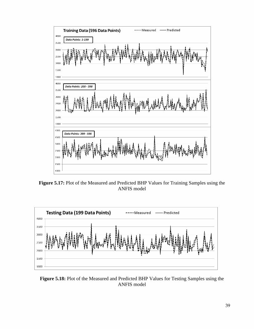
Figure 5.17: Plot of the Measured and Predicted BHP Values for Training Samples using the
ANFIS model ............................................................................................................................ 39

viii
Figure 5.18: Plot of the Measured and Predicted BHP Values for Testing Samples using the
ANFIS model ............................................................................................................................ 39
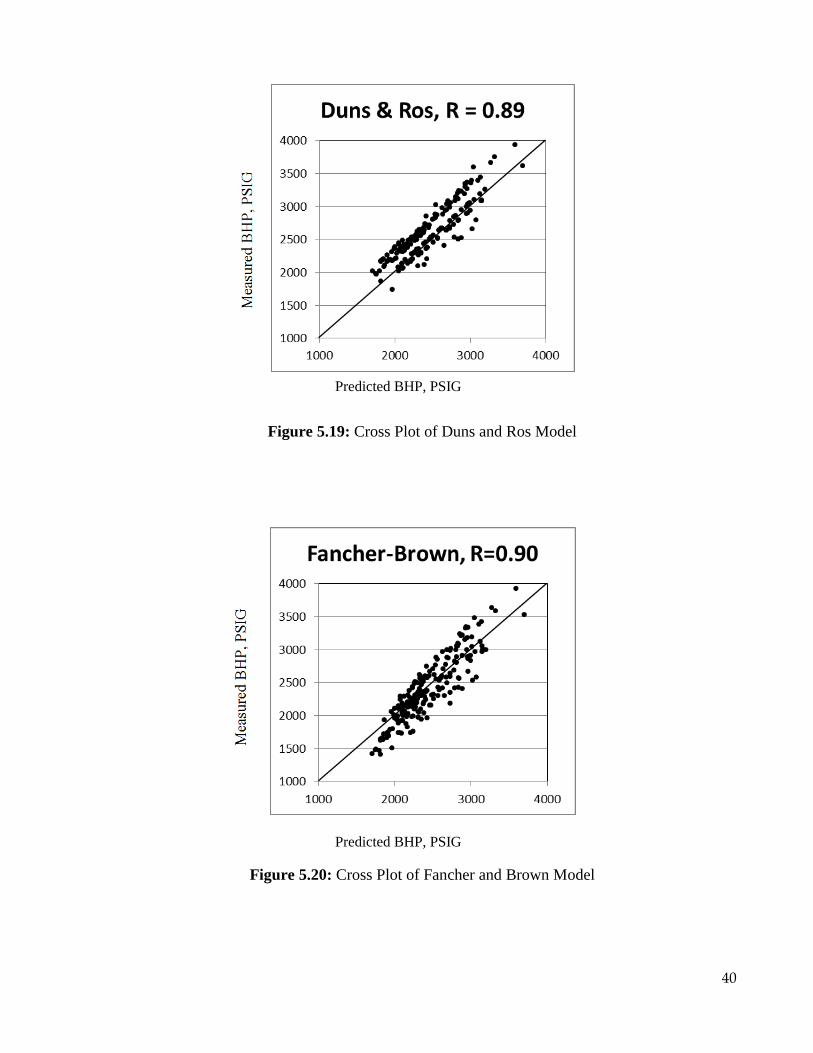
Figure 5.19: Cross Plot of Duns and Ros Model ..................................................................... 40
Figure 5.20: Cross Plot of Fancher and Brown Model ............................................................ 40
Figure 5.21: Cross Plot of Hagedorn and Brown Model ......................................................... 41
Figure 5.22: Cross Plot of Orkiszewski Model ....................................................................... 41
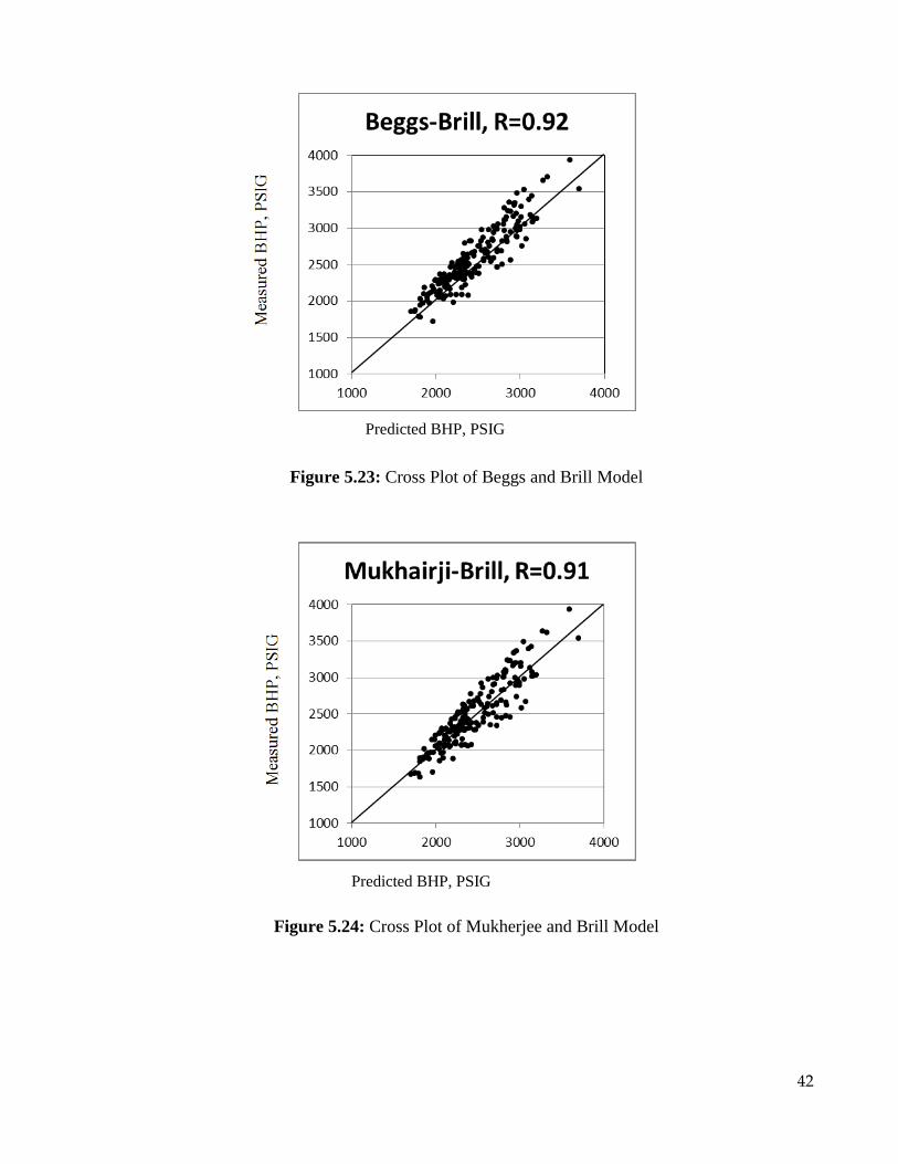
Figure 5.23: Cross Plot of Beggs and Brill Model .................................................................. 42
Figure 5.24: Cross Plot of Mukherjee and Brill Model ........................................................... 42
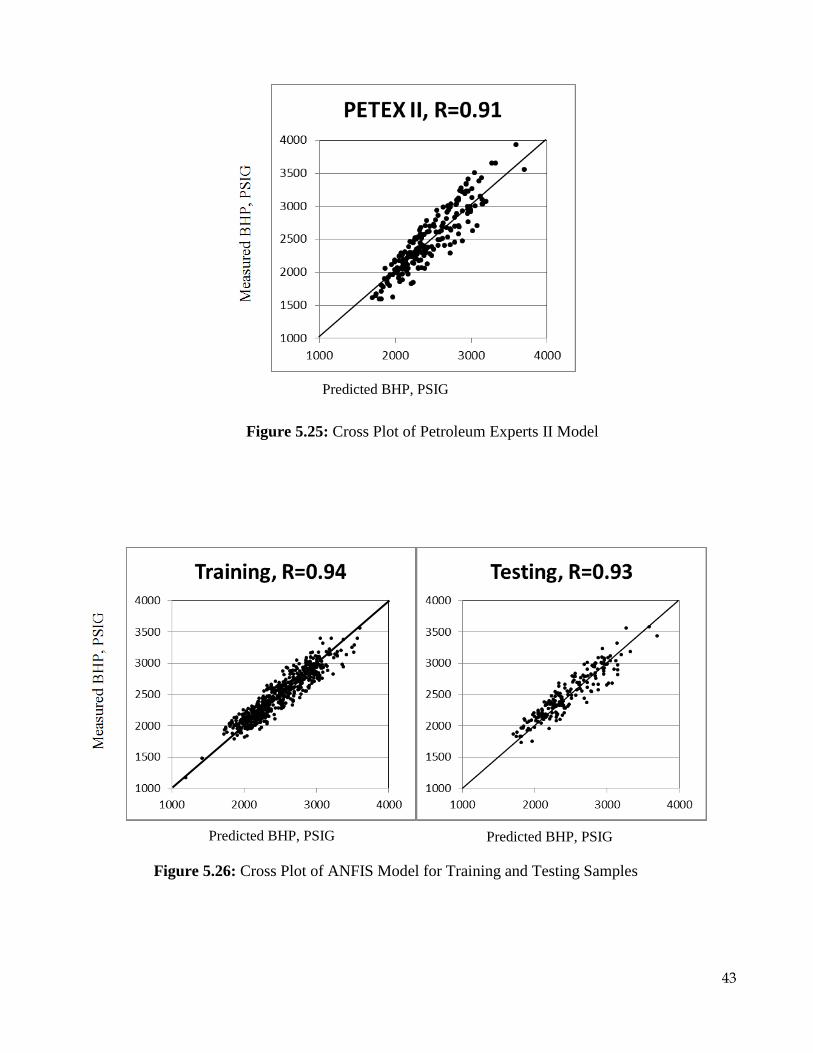
Figure 5.25: Cross Plot of Petroleum Experts II Model .......................................................... 43
Figure 5.26: Cross Plot of ANFIS Model for Training and Testing Samples ......................... 43
Figure 5.27:Histogram of Relative Error Distribution for the Developed ANFIS Model using
the Training Sets Results .......................................................................................................... 45
Figure 5.28: Histogram of Relative Error Distribution for the Developed ANFIS Model using
the Testing Sets Results ............................................................................................................ 45
Figure 5.29: Histogram of Relative Error Distribution for Dun-Ros Model ........................... 46
Figure 5.30: Histogram of Relative Error Distribution for Hagedorn-Brown Model ............. 46
Figure 5.31: Histogram of Relative Error Distribution for Fancher-Brown Model ................ 47
Figure 5.32: Histogram of Relative Error Distribution for Mukherjee-Brill Model ............... 47
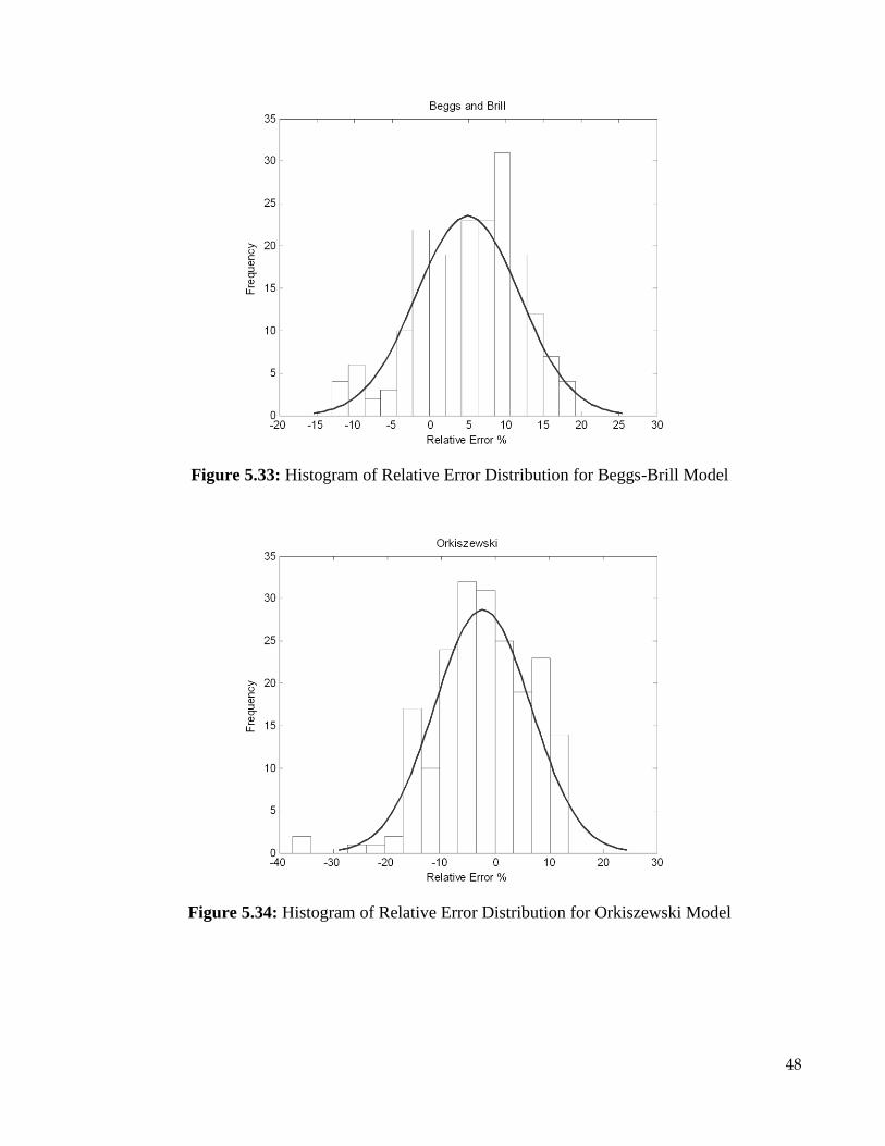
Figure 5.33: Histogram of Relative Error Distribution for Beggs-Brill Model ....................... 48
Figure 5.34: Histogram of Relative Error Distribution for Orkiszewski Model ..................... 48
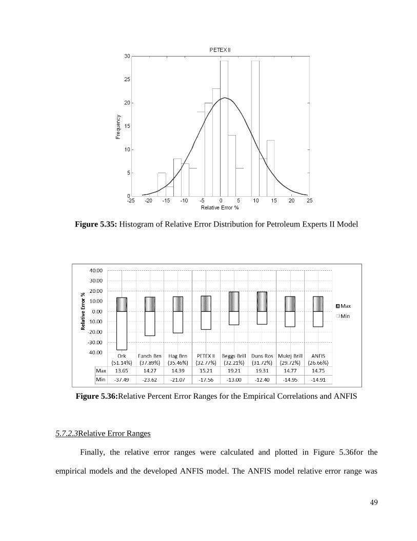
Figure 5.35: Histogram of Relative Error Distribution for Petroleum Experts II Model ........ 49
Figure 5.36:Relative Percent Error Ranges for the Empirical Correlations and ANFIS ......... 49

ix
List of Tables
Table 5.1: Collected Data Ranges of Input and Output Parameters ........................................ 22
Table 5.2: Collected Data Ranges of Input and Output Parameters for Training and Testing 22
Table 5.3: Statistical Analysis Results of the Empirical Correlations and the ANFIS model . 35

x
THESIS ABSTRACT
NAME OF STUDENT : Ahmad Tariq Al-Shammari
TITLE : Prediction of Pressure Drop for Two-Phase Flow in Vertical
Pipes using Artificial Intelligence
MAJOR FIELD : Petroleum Engineering
DATE OF DEGREE : December 2011
One of the significant parameters affecting flow rate in oil production wells is the
pressure drop between the well bottom-hole and tubing head. The pressure drop calculation in
two-phase flow systems is very complicated due to the variations in gas and liquid flow rates
across the two-phase flow stream. As the pressure of crude decreases while climbing a well
tubular, more gas comes out of solution. This gradual increase in gas volumes leads to the
reduction of liquid slip velocity and creating new flow patterns that are not only different in
shape, but also complicated in pressure drop calculations. To overcome this difficulty in
calculating pressure drop in two-phase flow systems, scientists came up with two main
approaches: flow correlations and mechanistic models. These two approaches are applicable
within certain conditions and their accuracy in pressure drop prediction degrades outside their
design boundary ranges.
The raising popularity of Artificial Intelligence (AI) techniques during the past two
decades proved that AI can be an alternative solution to many of the complicated problems
where physics and classic statistics fail to provide satisfactory solutions. These techniques
applied in different upstream fields have provided fast, robust and reliable numerical models
xi
in a variety of areas, e.g., geological modeling, reservoir engineering, petrophysics and well
testing. This thesis describes the utilization of Fuzzy Logic, which is one of the famous AI
techniques, in predicting flowing bottom-hole pressure in oil producer wells. Real well testing
data from the Middle East were used in constructing the Fuzzy Logic model. After training
the model using 596 well testing data samples, it was successfully able to predict the flowing
bottom-hole pressure at 199 well testing samples with an average absolute error of 4.9%. A
comparison analysis was conducted to evaluate multiple flow correlation in predicting
flowing bottom-hole pressure and compare their results with the developed Adaptive Neuro-
Fuzzy Inference System (ANFIS) model.

xii
ملخص الرسالة اسم اللطالب : أحمد طارق الشمري
عنوان الرسالة : التنبؤ بانخفاض الضغط للتدفق ثنائي الطور في اإلنابيب العمودية باستخدام الذكاء االصطناعي
التخصص : هندسة البترول
تاريخ التخرج : هـ 3311صفر
بار النفط يعد من أهم العوامل التي تؤثر بشكل مباشر في مقدار التدفق. الضغط بين قعر البئر وفوهته في آ إن مقدار انخفاض
لكن حساب مقدار انخفاض الضغط في التدفق ثنائي الطور يعتبر من العمليات المعقدة بسبب التغير في نسب الغاز والسائل عبر أنبوب
ن السائل وذلك بشكل تصاعدي مما ينتج معه خلق البئر العمودي، حيث أن انخفاض الضغط يتسبب في زيادة نسب الغاز المتحررة م
أنماط تدفق جديدة. هذه األنماط هي ليست مختلفة فقط بالشكل ، ولكن أيضا في العوامل المؤثرة في هبوط الضغط. للتغلب على هذه
لتدفق و النماذج ل ياضيةالعالقات الررئيسيين: أسلوبينالصعوبة في حساب انخفاض الضغط في التدفق ثنائي الطور، استخدم العلماء
قابالن للتطبيق ضمن نطاقات معينة ودقتهما في التنبؤ بانخفاض الضغط تقل خارج هذه النطاقات. األسلوباناآللية. هذان
(خالل العقدين الماضيين أن هذه الطريقة الرياضية يمكن أن توفر حلوال فعالة AIأثبتت زيادة شعبية الذكاء االصطناعي )
اكل المعقدة التي تفشل الفيزياء الكالسيكية والطرق اإلحصائية في حلها. وقد وفرت هذه التقنيات نماذج رقمية سريعة لكثير من المش
وموثوق بها في العديد من المجاالت كالتمثيل الجيولوجي، هندسة المكامن، الفيزياء النفطية وفحص اآلبار.
عد من أهم التقنيات في الذكاء االصطناعي، في التنبؤ بقيمة الضغط هذه األطروحة تشرح استخدام المنطق الضبابي، والذي ي
مجموعة من البيانات الحقيقية المأخوذة من دراسات 695في قعر اآلبار المنتجة النفط. ولبناء نموذج المنطق الضبابي استخدمت
مجموعة من البيانات 999قعر البئر لـ فحص اآلبار آلبار من الشرق األوسط. وكان النموذج قادرا على التنبؤ بقيمة الضغط في
% . وأجري تحليل مقارنة 9.9األخرى التي استخدمت لفحص دقة النموذج الضبابي والتي نتج عنها مقدار خطأ متوسط مطلق يعادل
ارنة أداء هذه بين نموذج المنطق الضبابي والعديد من نماذج ارتباطات التدفق الشهيرة للتنبؤ بقيمة الضعط في قعر البئر وذلك لمق
(ANFISالنماذج مع طريقة "نظام االستدالل العصبي الضبابي المتكيف" )
درجة ماجستير العلوم
جامعة الملك فهد للبترول والمعادن
المملكة العربية السعودية –الظهران
هـ 3311صفر : التاريخ

CHAPTER 1
INTRODUCTION
Two phase flow is an expression that refers to systems containing simultaneous flow of
gas and liquid. Historically, this type of flow has been studied in power systems, in which
pressurized water along with steam flow together in boilers and heat exchangers. Moreover, flow
of steam and water is studied in nuclear reactors that utilize water for cooling reactor cores. In the
petroleum industry, the two phase flow behavior grasp great attention as it affects the whole oil
and gas production system from the reservoir up to the refinery.
Petroleum fluid is composed of multiple organic components that vary in molecular
weight. The molecular weights and mass percentages of these components within a petroleum
reservoir fluid define its properties such as density, viscosity and bubble point pressure, below
which gas phase start to appear as a separate fluid.
In oil reservoirs with pressures above the bubble point, the main fluid phase is liquid
regardless of the percentage of the gas phase that is in solution. However, as the crude enters the
wellbore, the pressure starts decreasing vertically until the bubble point pressure is reached. The
gradual decrease in the pressure within a production tubing results in releasing greater amounts of
gas bubbles that start slipping over the liquid phase and accumulating to form larger bubbles or
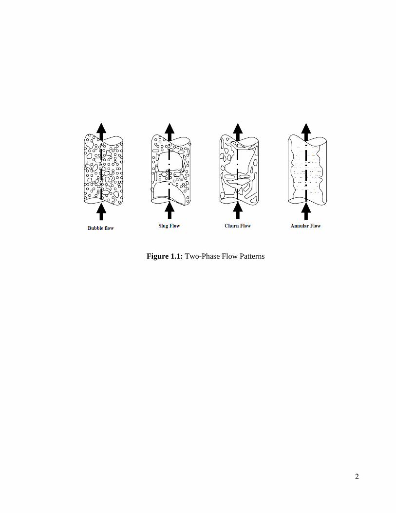
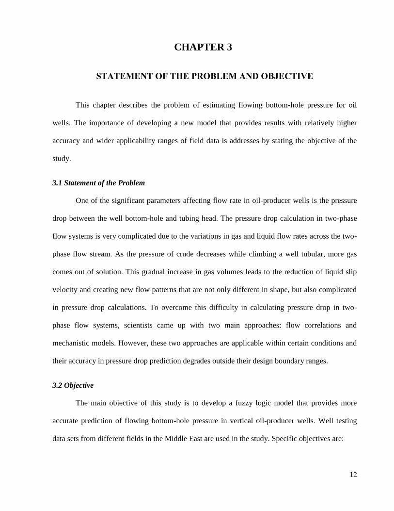
slugs and new flow patterns will appear as illustrated in Figure 1.1.
2
Figure 1.1: Two-Phase Flow Patterns

3
As a result of forming the different flow patterns in oil-producer wells, the pressure drop
calculations are complicated and require deep understanding of many parameters such as liquid
holdup, mixture density, two-phaseReynoldsnumber…etc.Thepressure drop prediction however
is very important for petroleum engineers. Pressure losses in oil and gas wells are used in
designing tubing sizes, completion configurations, and artificial lift requirements and to predict
the flowing bottom-hole pressure.
The utilization of Artificial Intelligence (AI) techniques in the petroleum industry has
gained a considerable attention during the past few decades. These techniques have provided
solutions to a large number of problems in determining several geological, petro-physical and
petroleum engineering parameters that are difficult to tackle using classical physics or
engineering concepts. The present study focuses mainly on developing a new Fuzzy Logic model,
which is one of the important AI techniques, to be used in predicting pressure for vertical oil-
producer wells.
The report is composed of six chapters. Chapter 2 focuses on the literature review that
briefly describes the approaches of pressure drop calculations in two phase flow systems and the
use of fuzzy logic in the petroleum industry. Chapter 3 presents the statement of the problem and
defines the general objectives. In Chapter 4, the basic concepts of Fuzzy Logic and the Adaptive
Neuro-Fuzzy Inference System are presented. The results and analysis discussions are described
in detail in chapter 5, and finally, the conclusions and recommendations are stated in Chapter 6.

4
CHAPTER 2
LITERATURE REVIEW
Fluid flow rate in a pipe is directly proportional to the pressure difference between the
pipe inlet and outlet. Considering a pipe with fixed inside diameter and fluid flow under steady-
state conditions, there are two main types of pressure losses: gravitational and frictional. This
chapter discusses the main concepts and equations for determining pressure drop in oil wells. In
addition, a section that reviews the application of Fuzzy Logic in the petroleum industry is added.
2.1 Gravitational Pressure Drop
Gravitational pressure drop occurs only if there is a change in elevation between a pipe
inlet and outlet. Gravitational pressure difference is directly proportional to the vertical elevation
change and the fluid specific gravity. The amount of pressure drop in field units due to gravity
can be calculated using equation12-1:
)1.2.......(......................................................................sinθ L SG 0.433(psi)ΔP mGravity
Where: SGm is the mixture specific gravity, L is tubing depth (ft) and is the inclination
angle
In oil producer wells with low to average GOR values, the gravitational pressure drop is
the major contributor to the total pressure losses between a well sand-face and tubing head. In oil
wells with GOR values around500 scf/bbl, 80 – 85% of the total pressure drop is due to
1“SamiAl-Nuaim,classlecturefor“AdvancedWellPerformance”,KFUPM,March,2009”

5
gravitational losses and the rest would be mostly frictional. As the GOR increases, frictional
pressure losses start to dominate the total pressure drop due to the increase in fluid mixture
velocity and the reduction of liquid holdup.
2.2 Frictional Pressure Drop
Frictional pressure loss occurs due to shear forces acting against fluid flow direction. The
frictional losses happen near the pipe inner surface due to the molecular interconnectivity forces
that resist the deformation. These forces are directly proportional to the kinetic energy of the fluid
element and to the friction factor, which can be determined experimentally. Several scientists
tried to correlate the friction factor with different flow parameters.
In 1944, Lewis Moody published“FrictionFactorforPipeFlow”(1).TheworkofMoody
has become the basis for many of the calculations on friction loss in pipes. Colebrook and White
came up with an implicit relationship (Equation 2.2) for calculating friction factor (2).
..................................................................................).........7.182
log(274.11
Re fNdf
(2.2)
This equation was then solved by Swamee and Jain (3) to give an explicit approximated
solution as in equation 2.3:
.......................................................................................).........25.21
log(214.11
9.0
ReNdf
(2.3)
Whereεtheabsolutepiperoughness(ft),disthepipediameter(ft)andNRe is Reynolds number
The pressure drop due to friction in single phase can be calculated as2:
( )
………………………..……..………………(2.4)
2 “SamiAl-Nuaim,classlecturefor“AdvancedWellPerformance”,KFUPM,March,2009”
6
Where: is the single phase fluid density (lb/ft^3), f is the friction factor (dimensionless),
L is tubing depth (ft), q is flow rate (bpd) and d is tubing diameter (in)
2.3 Pressure Drop Calculations in Oil Producer Wells
As described above, the total pressure drop in oil wells is mainly composed of
gravitational and frictional pressure drops. In order to calculate the total pressure drop along a
production tubing section, one needs to determine the amounts of gas and liquid and trace their
changes vertically. The vertical flow inside a tubing section is accompanied with pressure
reduction and as the pressure reaches the bubble point, gas bubbles begin to be released. These
bubbles slip vertically through the liquid column and start to accumulate as more bubbles are
formed with the pressure decrease. The accumulation of gas bubbles results in forming larger
bubbles that grow more as the flow climbs the tubing section, creating what is called slug flow.
As the pressure continues to decrease and yet more gas is still to be released out of solution, the
gas phase might transform into continuous phase at the center of the pipe and oil phase will flow
as a thin fluid ring on the inside wall of the tubing. These different fluid-gas phase patterns are
known as flow regimes, which are predicted based on empirical formulas that were mostly
developed numerically in the lab. It is obvious that both gravitational and frictional pressure
losses will be different depending on the flow regime type, which results in complicating the
approaches for calculating total pressure drop in oil wells.
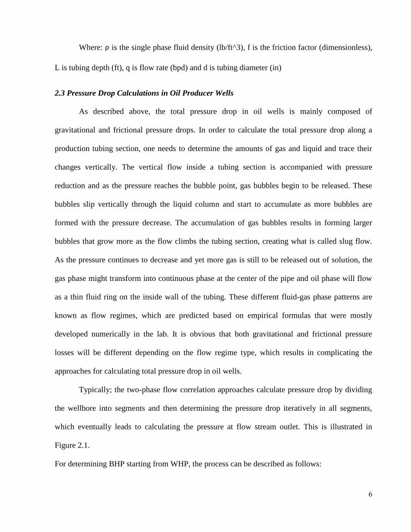
Typically; the two-phase flow correlation approaches calculate pressure drop by dividing
the wellbore into segments and then determining the pressure drop iteratively in all segments,
which eventually leads to calculating the pressure at flow stream outlet. This is illustrated in
Figure 2.1.
For determining BHP starting from WHP, the process can be described as follows:

7
1. Divide the wellbore into segments.
2. Assume P2 at the first segment outlet.
3. Calculate average pressure of the segment based on P1 and assumed P2.
4. Calculate GOR and FVF for Oil & Gas at Pave to come up with liquid holdup.
5. Determine flow pattern based on holdup and inclination angle.
6. Calculate two phase density at Pave.
7. CalculateΔP gravity.
8. Find Reynolds number and friction factor.
9. CalculateΔP friction.
10. The pressure at outlet P2 is calculated based on P2 = P1 – Δ P total.
11. Compare calculated P2 with the initially assumed P2. If they match within a tolerance, then
consider P2 to be the inlet pressure for the subsequent segment. Otherwise, consider P2
(assumed) = P2 (calculated) and go to step #2.
8
Figure 2.1: Pipe segmentation to calculate pressure drop iteratively
9
The previous steps indicate the complexity in calculating pressure drop for oil producer
wells using two-phase flow correlations. Most of the computation steps involve the utilization of
empirical correlations that were developed based on statistical and curve fitting techniques.
Majority of the developed two-phase flow correlations and mechanistic models were
constructed with limited conditions and their error in predicting pressure drop tends to increase as
the conditions start deviating from the design boundaries. There is no available single correlation
or mechanistic model that can be applicable for all ranges of production such as GOR, liquid rate,
tubing size or watercut. (4)
Recently, there were some studies that started tackling calculating pressure drop in two-
phase flow systems using one of the Artificial Intelligence techniques which is the Artificial
Neural Networks. In 1995, Terniyik, Bilgesu and Mohaghegh introduced the implementation of
ANN in calculating flowing bottom-hole pressure in vertical and inclined pipes. They called this
methodology: Virtual Measurement in Pipes (VMP). They used two sets of data and developed
two separate neural network models. The first one was with pressures ranging between 100 and
10,000 psig and second was for pressure values less than 100 psig (5). In 2005, Osman, Ayoub
and Aggour used neural networks in predicting bottom-hole pressures for vertical wells. They
used initially a total of 386 field data sets published by Al-Muraikhi et al and collected from
Middle East fields. They first tested the data against multiple empirical correlations and
mechanism models and removed data sets that were poorly modeled by all correlations and
models.Afterremovingthe“outliers”,206datapointswerethenusedtodevelopandANNmodel
(6). A very similar recent study was introduced by Mohammadpoor et.al. in 2010 based on
Iranian well test data. They also used ANN to predict flowing bottom-hole pressure (7).
10
2.4 The Use of Fuzzy Logic in the Petroleum Industry
Fuzzy Logic has been used in several petroleum engineering-related applications. These
include petrophysics and permeability determination, stimulation candidate selection, production
optimization and completion and multilateral design.
In 2000, S.J Cuddy (8) described the application of Fuzzy Logic in determining litho-facies and
permeability in un-cored wells. In his study, he used data for 10 cored wells to derive litho-facies
and permeability in 30 un-cored wells.
Ali Garrouch, et. al. of Kuwait University (9) developed in 2003 a new Fuzzy Logic for designing
optimal multilateral well configuration and completion. They formulated reservoir candidate
screening criteria for applying multilateral technology, and implemented these criteria in a new
expert system that features the use of fuzzy logic for handling ambiguity in completion scenarios.
Similar to Cuddy methodology in finding permeability, in 2005, M. Amabeoku et. al. published a
paper describing the use of Fuzzy Logic to model and predict permeability in cored wells by
calibrating core permeability against conventional open-hole logs (10). The permeability models
developed were then used to generate permeability trace in each well across a field.
Fuzzy logic was also used to predict reservoir fluid viscosity. In 2007, Yasin Hajizadeh published
this work which included using both ANN and fuzzy logic in predicting oil viscosity (11). He
used both techniques to recognize the pattern between the given data sets where this patter may
not be understood clearly or no precise mathematical relationship exists.
One of the recent studies that utilized Fuzzy Logic modeling was to determine inflow
performance relationship in horizontal oil wells. This study was conducted by Ebrahimi, M in
2010 (12). The author tried two neuro-fuzzy models, including Local Linear Neuro-Fuzzy Model
and Adaptive Neuro Fuzzy Inference System and compared the performance with empirical

11
correlations to predict inflow performance of horizontal oil wells experiencing two phase flow.
The prediction of flowing bottom-hole pressure
12
CHAPTER 3
STATEMENT OF THE PROBLEM AND OBJECTIVE
This chapter describes the problem of estimating flowing bottom-hole pressure for oil
wells. The importance of developing a new model that provides results with relatively higher
accuracy and wider applicability ranges of field data is addresses by stating the objective of the
study.
3.1 Statement of the Problem
One of the significant parameters affecting flow rate in oil-producer wells is the pressure
drop between the well bottom-hole and tubing head. The pressure drop calculation in two-phase
flow systems is very complicated due to the variations in gas and liquid flow rates across the two-
phase flow stream. As the pressure of crude decreases while climbing a well tubular, more gas
comes out of solution. This gradual increase in gas volumes leads to the reduction of liquid slip
velocity and creating new flow patterns that are not only different in shape, but also complicated
in pressure drop calculations. To overcome this difficulty in calculating pressure drop in two-
phase flow systems, scientists came up with two main approaches: flow correlations and
mechanistic models. However, these two approaches are applicable within certain conditions and
their accuracy in pressure drop prediction degrades outside their design boundary ranges.
3.2 Objective
The main objective of this study is to develop a fuzzy logic model that provides more
accurate prediction of flowing bottom-hole pressure in vertical oil-producer wells. Well testing
data sets from different fields in the Middle East are used in the study. Specific objectives are:

13
1- To construct an Adaptive Neuro-Fuzzy Inference System (ANFIS) to predict flowing
bottom-hole pressure in vertical multiphase flow
2- To test the developed model against actual field data
3- To compare the performance of the developed model against several famous empirical
correlations.
14
CHAPTER 4
FUZZY LOGIC
In this chapter, we briefly discuss the main concepts of fuzzy logic, the degree of
membership and membership functions, the fuzzy (if-then) rules, the fuzzy inference system (FIS)
and finally, the adaptive neuro-fuzzy inference system (ANFIS).
4.1 What is Fuzzy Logic?
Theterm“Fuzzy”refersusuallytouncertainty,ambiguityor something not well defined.
Most of the natural physical properties can be described by non-crisp terms such as hot, cold,
bright,hard,strong…etc.Thehumanthinking,reasoninganddecisionmakingprocessesarealso
not crisp. We use vague, imprecise words to explain our thoughts or communicate with one
another (13). Fuzzy systems are usually used to represent uncertainty that is caused by inaccuracy
or ambiguity of the data or lack of the input parameters that have important influence on results.
In fuzzy systems, an item or a property can be described by classifying it under one of different
non-crisp sets in addition to a degree of membership to each set. (14)
The concept of Fuzzy Logic evolved from the fuzzy set theory that was proposed by a
mathematician of Iranian descent: Dr. Lotfi A. Zadeh in 1965. Dr. Zadeh is considered the father
of Fuzzy Logic and its implementations in mathematics, computer sciences, system control and
artificial intelligence. The fuzzy set theory suggests dealing with non-crisp variables by adding a
truth value that ranges between 0 and 1(15).The relation between a variable and its truth value can
be described by a “membership” function that ranges between 0 and 1 and the value of this
variable in the functions defines a“degree”ofmembership.
15
4.2 Degree of Membership and Membership Functions
Let us take for example an AC temperature setting and define the human feeling at each
temperature as different fuzzy sets. We could consider 16oC to be cold, 22
oC as pleasant and 26
oC
as hot. The three sets here are: cold, pleasant and hot and each temperature setting can belong to
one of these sets at a degree of membership. Take for example, the temperature 25oC, is it
pleasant or hot? Actually, it can belong to the two sets at the same time but with different degree
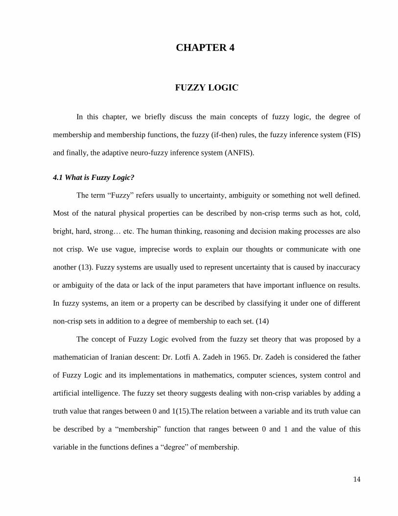
of membership. We can say that it is not very pleasant or it is a little hot. This can be described
graphically in Figure 4.1, where the membership value of 25oC is 0.75 with Pleasant property and
0.25 with Hot property.
One way of representing fuzzy set and membership information is µA(x) = m, where the
membership µ of an item x in a fuzzy set A is m. The AC temperature example can be expressed
by the following expression: µHot(25) = 0.75 or µPleasant(25) = 0.25
In fuzzy logic, unlike representing a normal set like A = {x | x is even number}, we
describefuzzysetsbycouplingelementswithmembershipfunctionssuchasA={x,µA(x)|xє
X}. The membership functions can be simple straight lines or advanced functions such as
trapezoidal, sigmoid or Gaussian. (8)
4.3 Fuzzy If-Then Rules
When the conditional statements “ ” are characterized by membership
functions, they are called fuzzy if-then rules. An example that can explain this type of rules is:
When volume is large, then density is low, where volume and density are linguistic variables,
large and low are linguistic values that are associated with membership functions. (16)

16
Figure 4.1: Describing Temperatures using Fuzzy Sets
knowledge base
(fuzzy)
fuzzification
Interface
defuzzification
Interface
decision-
making unit
database rule base
Input(crisp) Output(crisp)
(fuzzy)
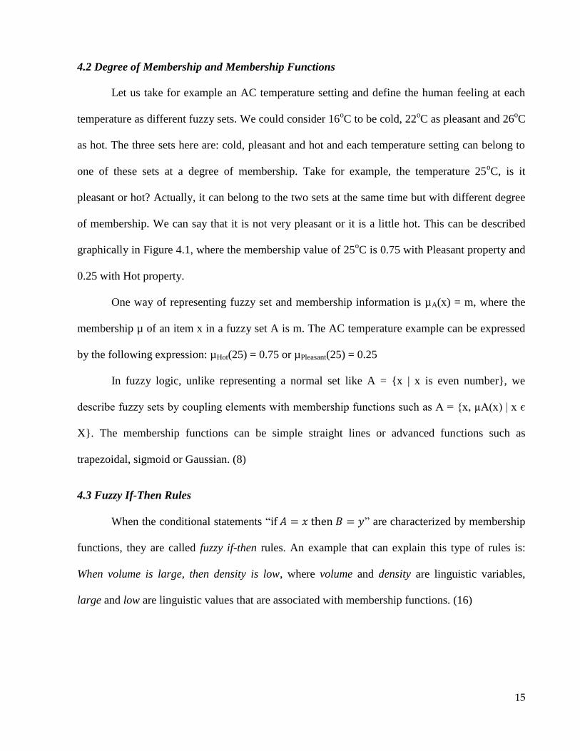
Figure 4.2: Fuzzy Inference System (FIS) Blocks, ref:(16)

17
Another type of fuzzy if-then rules is the Sugino-type, which includes fuzzy sets only in
the premise part. An example of this type of if-then rules is: If you are above 15, then your body
mass index (BMI) = weight / height^2, where the premise part has the term above 15, which is a
fuzzy set and the consequent part is described by a non-fuzzy set. (16)
4.4 Fuzzy Inference Systems
Fuzzy Inference System (FIS) is the process of establishing formulated mapping from an
input to an output using fuzzy logic. FIS involves combing formulating membership functions,
logicaloperationsandagroupof“If-Then”rules tocreateamatrixof rulesbetween inputsets
and an output.
Fuzzy inference systems are composed of five main blocks (see Figure 4.2):
1- Fuzification interface to transfer the crisp data inputs into degrees of match with linguistic
values
2- Rulebase,whichcontainsanumberoffuzzy“if-then”rules
3- Database for the membership functions of the fuzzy sets used in the rules
4- Decision making unit, which is used for the inference operations
5- Defuzzification interface, to transfer the fuzzy output into crisp results. (16)
The fuzzy inference operations include first“fuzzifying”theinputvariablesbyassigninga
degree of truth between 0 and 1 to statements about the input variables in the antecedent (IF) part
of the rules. The degrees of truth are determined by the membership functions. These statements
are also joined by connectives (AND or OR) and the fuzzy operator resolves the overall
antecedent based on the connections used. The fuzzy operator converts all the logical statements
into a number between 0 and 1. (17)

18
4.5 Adaptive Neuro-Fuzzy Inference System (ANFIS)
ANFISmethodprovidesatechniqueforfuzzymodelingprocessto“learn”fromdatasets.
This method is applied to construct a FIS and tuning or adjusting the membership functions using
back propagation algorithms along with least-square type functions to learn from datasets. A
structure similar to neural networks is created to map inputs using input membership functions
and associated parameters, and then through output membership functions and associated
parameters to the outputs. ANFIS is used for constructing a set of fuzzy “if-then” rules with
membership functions to generate input-output pairs. (17)
4.5.1 ANFIS Architecture
Let us consider a fuzzy inference system with two inputs x and y and one output z.
Suppose that the rule base contains two fuzzy if-then rules. (16)
Rule 1: if x is a1 and y is b1, thenf1 = p1 x + q1 y + r1……………………..……..(4 . 1)
Rule 2: if x is a2 and y is b2, thenf2 = p2 x + q2 y + r2……………………..……..(4 . 2)
Where fiis the consequent function, pi, qiand riare the consequent parameters.
The ANFIS structure is composed of 5 basic layers and each layer is composed of nodes that are
equal to the number of rules.
Layer 1: This layer includes fuzzifying the input and establishing the membership degree
for each rule to one of the “bell-shape”membershipfunctions. An example of this
representation is as follows:
( ) { (
)
} ………..………………………….……….(4 . 3)
Where , are the membership function parameters set that are modified
during the learning process to provide acceptable output.
19
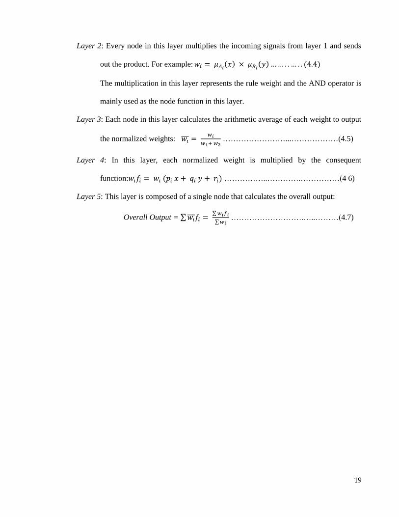
Layer 2: Every node in this layer multiplies the incoming signals from layer 1 and sends
out the product. For example: ( ) ( ) ( )
The multiplication in this layer represents the rule weight and the AND operator is
mainly used as the node function in this layer.
Layer 3: Each node in this layer calculates the arithmetic average of each weight to output
the normalized weights: ̅̅ ̅
……………………...………………(4.5)
Layer 4: In this layer, each normalized weight is multiplied by the consequent
function: ̅̅ ̅ ̅̅ ̅ ( ) ……………..………….……………(4 6)
Layer 5: This layer is composed of a single node that calculates the overall output:
Overall Output = ∑ ̅̅ ̅ ∑
∑ ……………………….…..………(4.7)

20
CHAPTER 5
RESULTS AND DISCUSSIONS
In this chapter, data handling in terms of data collection and pre-processing is firstly
discussed. Then, a detailed discussion of the developed ANFIS model, including model features
and model optimization is presented. Next, a detailed trend analysis of the new developed model
is presented to examine whether the model simulates the physical behavior. This is followed by a
detailed discussion of the model superiority and robustness against the empirical correlations
included in the study. Finally, statistical and graphical comparisons of the developed model
against the correlations are presented.
5.1 Data Acquisition
Data preparation is one of the key steps in developing any AI technique. It is very important to
review the data and remove outliers before using it in constructing AI models. For the current
study a total of 1207 well productivity testing data sets were initially collected from several fields
in the Middle East. The data sets included several key input parameters that were later used in
constructing the ANFIS model. The input parameters selected were: flowing wellhead pressure,
liquid rate, watercut %, gas oil ratio, oil API, reservoir temperature, tubing inside diameter and
the gauge depth. The output value was the measured flowing pressure at gauge depth.
5.2 Data Preprocessing and Filtration
Well testing data is subject to uncertainty and inaccurate measurements, so it is important to
filter the data and exclude all the datasets that include one or more of these inaccurate readings

21
that might disturb the smoothness of the model learning process. The filtration process was done
by applying the following steps:
1. A small computer program was written to feed well testing conditions (data sets) into
Prosper software to calculate flowing bottom-hole pressure using multiple flow
correlations. The correlations used were: Beggs and Brill, Duns and Ros, Hagedorn and
Brown, Fancher and Brown, Mukherjee and Brill, Orkiszewski and Petroleum Experts II.
2. The relative absolute error between the predicted and measured flowing bottom-hole
pressure was calculated for each of the correlations.
3. The arithmetic average error for all the correlations was computed at each dataset.
4. Datasets at which the average error is more than 15% were excluded from the study.
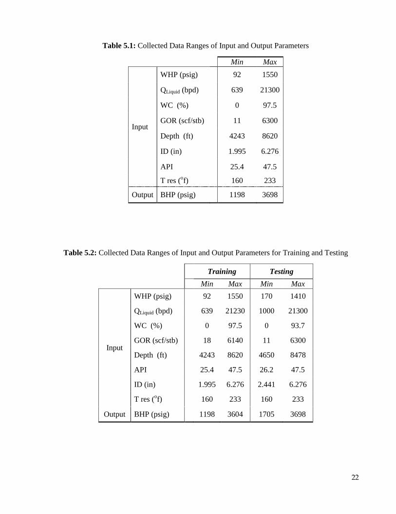
After filtering the data, we ended up having a total of 796 datasets. A summary of the data
parameter ranges is available in Table 5.1.
5.3 ANFIS Model Development
In this study, Matlab software was used for designing and optimizing the fuzzy logic
system. Matlab has a large library of functions and techniques that are used for constructing most
of the AI models. There are two main types of Fuzzy Inference Systems available: Mamdani and
Sugeno. In this study, we implemented Sugeno type FIS because it is more compact and has more
efficient representation of the rules. (17)
22
Table 5.1: Collected Data Ranges of Input and Output Parameters
Min Max
Input
WHP (psig)
92 1550
QLiquid (bpd)
639 21300
WC (%)
0 97.5
GOR (scf/stb)
11 6300
Depth (ft)
4243 8620
ID (in)
1.995 6.276
API
25.4 47.5
T res (of)
160 233
Output BHP (psig)
1198 3698
Table 5.2: Collected Data Ranges of Input and Output Parameters for Training and Testing
Training Testing
Min Max Min Max
Input
WHP (psig) 92 1550 170 1410
QLiquid (bpd) 639 21230 1000 21300
WC (%) 0 97.5 0 93.7
GOR (scf/stb) 18 6140 11 6300
Depth (ft) 4243 8620 4650 8478
API 25.4 47.5 26.2 47.5
ID (in) 1.995 6.276 2.441 6.276
T res (of) 160 233 160 233
Output BHP (psig) 1198 3604 1705 3698
23
The technique used in creating the FIS for this study was to implement subtractive
clustering method that groups the data into multiple clusters and each cluster is defined by a
radius of influence whose values range between 0 and 1. Small value of cluster radius results in a
larger number of rules and usually tends to over fit the train in data. Each value of the input
variables is then linked to a cluster by a membership function that is fine-tuned iteratively until
the model predicts an output with minimal deviation from target value.
Several FIS techniques were tested in Matlab to come up with the most optimized
technique. It was found that theMatlab function: “genfis2” provides superiormodeling results
during the training stage and hence used for further optimization. This function generates Sugeno-
type FIS structure using subtractive clustering of the data and extracts rules and membership
functions to model the data behavior (17).Among the 795 well testing data samples, 596 data
samples (75%) were used for training and 199 (25%) for testing. Table 5.2 summarized the ranges
for the training and testing data to insure most of the data ranges are similar in both.
5.4 Model Optimization
After testing several cluster radii, it was found that a cluster radius of 0.6 was the most
optimized value with an average absolute error of 4.33 % and 4.92% on the training and testing
data respectively. Figures 5.1 and 5.2 indicate the effect of cluster radius on the error standard
deviation, the average absolute error and correlation factor between predicted and measured BHP.
The figure indicates that small cluster radius has a good impact on predicting the BHP for the
training data samples (Figure 5.1). However, this results in a large number of rules that almost
memorized the data blindly, which has a bad influence on the prediction of the BHP using testing
samples (Figure 5.2).

24
Figure 5.1: Effect of Grid Size of ANFIS Performance (Training Samples)
Figure 5.2: Effect of Grid Size of ANFIS Performance (Testing Samples)

25
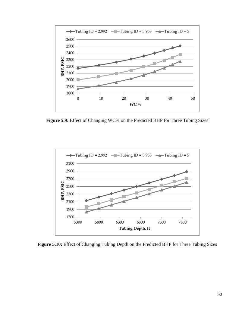
5.5 Trend Analysis
The trend analysis was carried out to check the physical behavior of the developed ANFIS
model. For this purpose, synthetic sets were prepared where in each set only one input parameter
was changed while other parameters were kept constant. To test the developed model, the effects
of gas oil ratio, oil rate, water cut%, tubing diameter, and tubing depth on flowing bottomhole
pressure were determined and plotted on Figures 5.3 through 5-6. Figure 5-3 indicates the effect
of increasing GOR on the predicted BHP. The ANFIS model predicted the expected trend of
decreasing BHP as the GOR increases because of the reduction in hydrostatic pressure in the
tubing. In Figure 5-4, the effect of increasing oil rate while keeping the water and gas rates along
with other conditions constant on bottomhole prediction is shown. This oil rate increase while
maintaining fixed water and gas rates results in increasing the total liquid rate and reducing the
GOR, which results in higher friction and larger hydrostatic head and to overcome this increased
frictional loss and hydrostatic column weight, the bottomhole pressure should increase. The
ANFIS models followed the general trend of the empirical correlations and provided the expected
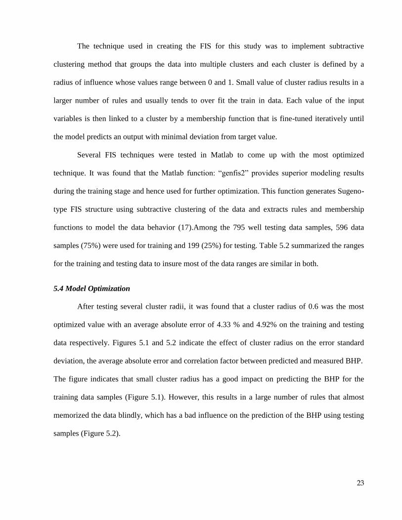
behavior. Figure 5.5 displays the effect of increasing water cut on the predicted bottomhole
pressure. The increase in water cut while keeping the oil rate constant results in increasing the
total liquid rate as well as increasing the hydrostatic column head, which results also in higher
bottomhole pressure. This general trend was also captured by the predicted bottomhole pressure
using the ANFIS model. Finally, the effect of tubing inside diameter is shown in Figure 5.6. As
the tubing size increases, the frictional pressure loss in the tubing decreases, which results in
lower bottomhole pressure. The general trend was captured by the model. However, the model
deviates from the overall trend at small tubing ID values. This behavior will be explained in the
next section that analyzes the grouped error analysis, in which we will notice that the error in

26
Figure 5.3: Effect of Gas Oil Ratio on Predicted BHP at: WHP=500 psig, WC=20%, QL=6000
bpd, Depth=6000 ft and Tubing ID=3.958 inches
Figure 5.4: Effect of Oil Rate on Predicted BHP at: WHP=500 psig, Qw=1200 bpd, Qg=5000
Mscf, Depth=6000 ft and Tubing ID=3.958 inches
27
Figure 5.5: Effect of Water Cut % on Predicted BHP at: WHP=500 psig, Qo=5000 bpd,
GOR=600 scf/bpd, Depth=6000 ft and Tubing ID=3.958 inches
Figure 5.6: Effect of Tubing ID on Predicted BHP at: WHP=500 psig, WC=20%, QL=6000 bpd,
GOR=600 scf/bpd and Depth=6000 ft

28
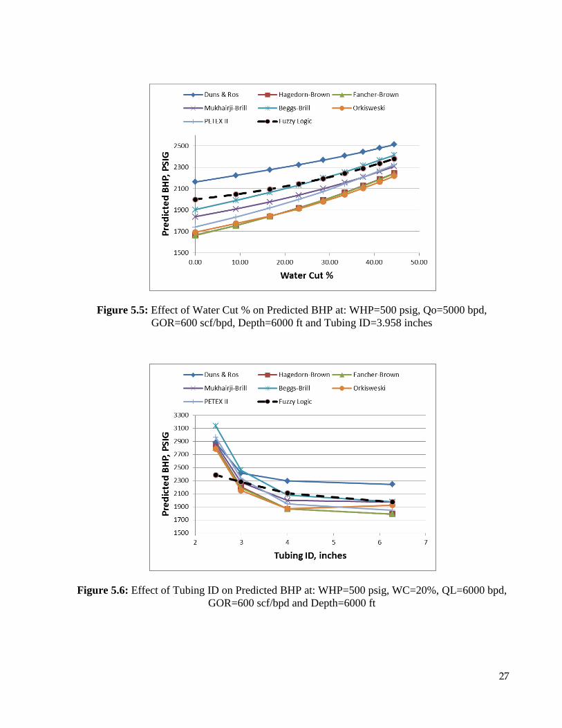
predicting bottomhole pressure using the ANFIS model is higher at smaller ID. To further
examine the ANFIS model validity, the trend analysis was checked at three different tubing sizes:
2.992, 3.958 and 5 inches. Figures 5.7 to 5.10 indicate the trend analysis for oil rate, GOR, WC%
and tubing depth respectively.
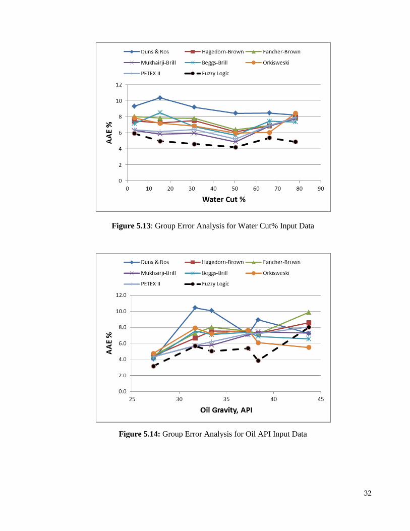
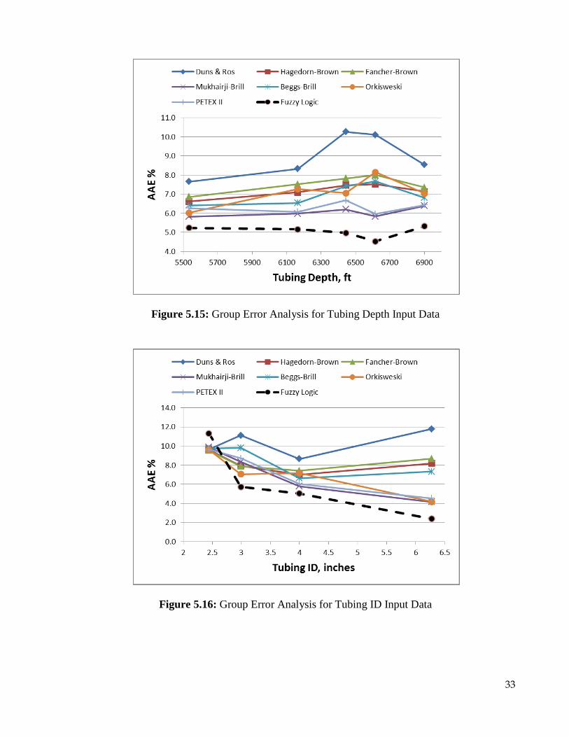
5.6 Group Error Analysis
Another statistical analysis was carried out to further evaluate the robustness of the
developed ANFIS model, which is the group error analysis. The group error analysis provides a
means for determining the strengths and weaknesses of the developed model and the empirical
correlations with respect to the input data. Some models provide good accuracy at certain input
data rangesandsomecouldhavepositiveornegativetrendsinthepredictedvalues’accuracyby
increasing or decreasing some input variables. The group error analysis is applied by grouping the
input parameters into few averaged sets and plotting the absolute average error at each set.
Figures 5.11 to 5.16 demonstrate the group error results plotted for the input parameters. The
figures indicates that the ANFIS model predicts BHP values with lower average absolute error
compared with the all the empirical correlations at all input parameter ranges except with respect
to the API and tubing ID ranges. We notice that the ANFIS model provides relatively larger
absolute error at API value of 44 and tubing ID of 2.441 inches and the reason for that is the small
number of data samples that were used in the training sets. If the number of training data samples
covering a certain data input value is small, then the combinations of the other different variables
may not be adequate to construct reliable set of rules.
29
Figure 5.7: Effect of Changing Oil Rate on the Predicted BHP for Three Tubing Sizes
Figure 5.8: Effect of Changing GOR on the Predicted BHP for Three Tubing Sizes
30
Figure 5.9: Effect of Changing WC% on the Predicted BHP for Three Tubing Sizes
Figure 5.10: Effect of Changing Tubing Depth on the Predicted BHP for Three Tubing Sizes
1800
1900
2000
2100
2200
2300
2400
2500
2600
0 10 20 30 40 50
BH
P,
PS
IG
WC %
Tubing ID = 2.992 Tubing ID = 3.958 Tubing ID = 5
1700
1900
2100
2300
2500
2700
2900
3100
5300 5800 6300 6800 7300 7800
BH
P,
PS
IG
Tubing Depth, ft
Tubing ID = 2.992 Tubing ID = 3.958 Tubing ID = 5

31
Figure 5.11: Group Error Analysis for Liquid Rate Input Data
Figure 5.12: Group Error Analysis for Gas Oil Ratio Input Data
32
Figure 5.13: Group Error Analysis for Water Cut% Input Data
Figure 5.14: Group Error Analysis for Oil API Input Data
33
Figure 5.15: Group Error Analysis for Tubing Depth Input Data
Figure 5.16: Group Error Analysis for Tubing ID Input Data

34
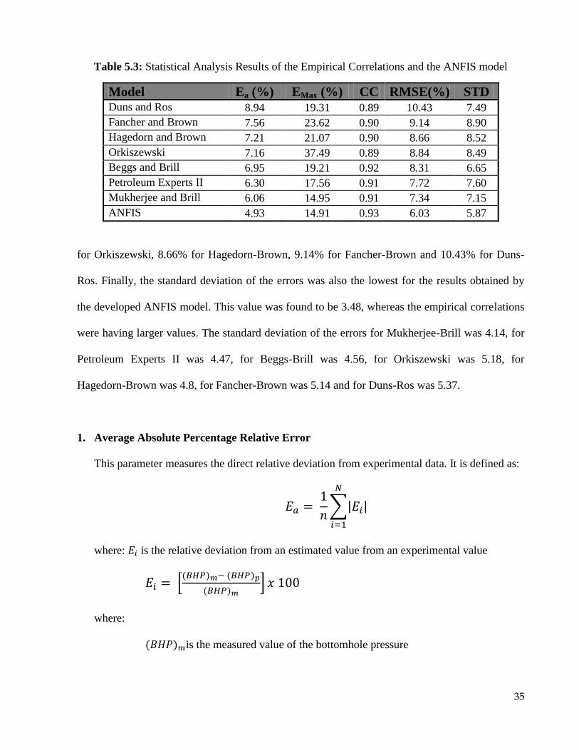
5.7 Statistical and Graphical Comparison
5.7.1 Statistical Error Analysis
The error analysis is used mainly as a basic tool for determining the robustness and
accuracy of the models. The statistical parameters included in the evaluation of the developed
model and the empirical correlations are: the average absolute percentage error, the maximum
absolute percentage error, the standard deviation of errors and the correlation coefficient between
predicted and actual BHP values. The equations for these parameters are given below. Summary
of the comparison between the empirical correlation and developed ANFIS model is presented in
Table 5.3. This table clearly indicates that the developed ANFIS model provided the best results
in all statistical parameters. The ANFIS model was able to predict BHP with an average absolute
error (Ea) of 4.93%, whereas the Ea values for the empirical models were: 6.06% for Mukherjee-
Brill, 6.3% for Petroleum Experts II, 6.95% for Beggs-Brill, 7.16% for Orkiszewski, 7.21% for
Hagedorn-Brown, 7.56% for Fancher-Brown and 8.94% for Duns-Ros correlation. The maximum
absolute percent error of 14.91%for the ANFIS model was also the lowest compared with the
empirical correlations. This maximum error for Mukherjee-Brill was 14.95%, for Petroleum
Experts II was 17.56%, for Beggs-Brill was 19.21%, for Orkiszewski was 37.49%, for Hagedorn-
Brown was 21.07%, for Fancher-Brown was 23.62% and for Duns-Ros was 19.31%. The
correlation coefficient between the actual and predicted BHP values was the highest for the
developed ANFIS model at a value of 0.93. This value was found to be 0.91 for both Mukherjee-
Brill and Petroleum Experts II, 0.92 for Beggs-Brill, 0.9 for both Hagedorn-Brown and Fancher-
Brown and 0.89 for both Orkiszewski and Duns-Ros. The root mean square error was also the
lowest for the ANFIS model at a value of 6.03%. The RMSE value for the empirical correlations
were: 7.34% for Mukherjee-Brill, 7.72% for Petroleum Experts II, 8.31% for Beggs-Brill, 8.84%
35
Table 5.3: Statistical Analysis Results of the Empirical Correlations and the ANFIS model
Model Ea (%) EMax (%) CC RMSE(%) STD Duns and Ros 8.94 19.31 0.89 10.43 7.49
Fancher and Brown 7.56 23.62 0.90 9.14 8.90
Hagedorn and Brown 7.21 21.07 0.90 8.66 8.52
Orkiszewski 7.16 37.49 0.89 8.84 8.49
Beggs and Brill 6.95 19.21 0.92 8.31 6.65
Petroleum Experts II 6.30 17.56 0.91 7.72 7.60
Mukherjee and Brill 6.06 14.95 0.91 7.34 7.15
ANFIS 4.93 14.91 0.93 6.03 5.87
for Orkiszewski, 8.66% for Hagedorn-Brown, 9.14% for Fancher-Brown and 10.43% for Duns-
Ros. Finally, the standard deviation of the errors was also the lowest for the results obtained by
the developed ANFIS model. This value was found to be 3.48, whereas the empirical correlations
were having larger values. The standard deviation of the errors for Mukherjee-Brill was 4.14, for
Petroleum Experts II was 4.47, for Beggs-Brill was 4.56, for Orkiszewski was 5.18, for
Hagedorn-Brown was 4.8, for Fancher-Brown was 5.14 and for Duns-Ros was 5.37.
1. Average Absolute Percentage Relative Error
This parameter measures the direct relative deviation from experimental data. It is defined as:
∑| |
where: is the relative deviation from an estimated value from an experimental value
[( ) ( )
( ) ]
where:
( ) is the measured value of the bottomhole pressure

36
( ) is the predicted value of the bottomhole pressure
2. Maximum Absolute Percentage Relative Error
This parameter measures the maximum relative deviation from among all data samples. It is
defined as:
| |
3. Correlation Coefficient
The correlation coefficient represents the degree of success in reducing the standard deviation.
It has a value ranging between It is given by:
√ ∑ [( )
( )
]
∑ [( ) ( ) ̅̅ ̅̅ ̅̅ ̅̅ ̅̅ ̅̅ ]
4. Root Mean Square Error:
The root mean square error measures the error dispersion around zero deviation. It is defined
by:
√∑
where: N is the number of testing samples.

37
5. Standard Deviation of Errors:
The standard deviation measures the dispersion or scattering of the data around the average
value. In this study, the standard deviation is calculated for the distribution of the relative errors
around the average relative error for each model. The equation is given by:
√∑( )
where: N is the number of testing samples.
Er is the relative error of the data, given by:
∑
5.7.2 Graphical Results Analysis
The graphical representation of the results provides a quick and adequate understanding of
the model prediction performance. In Figures 5.17 and 5.18, the measured and predicted BHP
values are plotted horizontally for all the training and testing samples to indicate the excellent fit
between them and demonstrate the robustness of the developed ANFIS model. To further analyze
the results graphically, additional representations are generated. This includes the cross-plot, the
error distribution histogram and the residual analysis.
5.7.2.1 Cross Plots
Cross-plots provide graphical representations of the correlation quality between the actual
and predicted BHP values. In this technique, all estimated values are plotted against the measured
values and thus a cross-plot is formed. A 45° straight line between the estimated versus actual
data points is drawn on the cross-plot, which denotes a perfect correlation line. The tighter the

38
cluster about the unity slope line, the better the agreement between the experimental and the
predicted results.
Figures 5.19 through 5.26 present cross-plots for the empirical correlations and the
developed ANFIS model. Investigation of these figures clearly shows that the developed ANN
model outperforms all the empirical correlations models. We notice that the cross-plot for Duns
and Ros model (Figure 5.19) indicates a general tendency towards under-predicting the BHP as
the majority of the results are above the 45ostraight line. The situation is the opposite in the case
of Fancher-Brown (Figure 5.20) and Hagedorn-model (Figure 5.21), where a larger portion of the
data are below the 45ostraight line in addition to a noticeable trend towards under predicting the
BHP values as they increase.
39
Figure 5.17: Plot of the Measured and Predicted BHP Values for Training Samples using the
ANFIS model
Figure 5.18: Plot of the Measured and Predicted BHP Values for Testing Samples using the
ANFIS model
40
Figure 5.19: Cross Plot of Duns and Ros Model
Figure 5.20: Cross Plot of Fancher and Brown Model
Predicted BHP, PSIG
Predicted BHP, PSIG

41
Figure 5.21: Cross Plot of Hagedorn and Brown Model
Figure 5.22: Cross Plot of Orkiszewski Model
Predicted BHP, PSIG
Predicted BHP, PSIG
42
Figure 5.23: Cross Plot of Beggs and Brill Model
Figure 5.24: Cross Plot of Mukherjee and Brill Model
Predicted BHP, PSIG
Predicted BHP, PSIG
43
Figure 5.25: Cross Plot of Petroleum Experts II Model
Predicted BHP, PSIG
Figure 5.26: Cross Plot of ANFIS Model for Training and Testing Samples
Predicted BHP, PSIG Predicted BHP, PSIG

44
Although these two models appear graphically similar in the cross-plot, there is a slight
difference between the two that is difficult to capture graphically. The cross-plot for Orkiszewski
model (Figure 5.22) provides a good representation of the results with a slight trend towards
under-estimating the BHP for larger values. The cross plots for both Mukherjee-Brill (Figure
5.24) and Petroleum Experts II (Figure 5.25) are reasonably very good compared with the
previously mentioned models with a correlation factor of 0.91 for both. However, the best
empirical model that provided larger value of the correlation coefficient and better even
distribution of the results above the below the 45o straight line is Beggs and Brill model (Figure
5.23) with a correlation coefficient value of 0.92. Figure 5.26 demonstrates the cross-plots for the
training and testing samples of the developed ANFIS model. The two plots indicate the excellent
match between the measured and predicted BHP values and the even distribution above and
below the 45o straight line.
5.7.2.2Error Distributions Histogram
The histogram of error distribution and the normal distribution curve provide means for
displaying the errors dispersal graphically to understand the performance of the model prediction
results. The errors are said to be normally distributed with a mean around the 0%. Figures 5.27
and 5.28 display the ANFIS model error distributions histogram and the normal distribution curve
applied for the training and testing data sets. Both plots indicate excellent behavior and normal
distribution around the 0% error. Comparing that with the empirical correlations, we notice that
the worse histogram distribution was for Duns and Ros model (Figure 5.29), which indicates a
clear shift towards an average error of +7 with weak normal distribution of the errors. The rest of
the empirical models provided reasonably better distribution histogram plots compared with Dun
and Ros model.

45
Figure 5.27:Histogram of Relative Error Distribution for the Developed ANFIS Model using the
Training Sets Results
Figure 5.28: Histogram of Relative Error Distribution for the Developed ANFIS Model using the
Testing Sets Results

46
Figure 5.29: Histogram of Relative Error Distribution for Dun-Ros Model
Figure 5.30: Histogram of Relative Error Distribution for Hagedorn-Brown Model

47
Figure 5.31: Histogram of Relative Error Distribution for Fancher-Brown Model
Figure 5.32: Histogram of Relative Error Distribution for Mukherjee-Brill Model
48
Figure 5.33: Histogram of Relative Error Distribution for Beggs-Brill Model
Figure 5.34: Histogram of Relative Error Distribution for Orkiszewski Model
49
Figure 5.35: Histogram of Relative Error Distribution for Petroleum Experts II Model
Figure 5.36:Relative Percent Error Ranges for the Empirical Correlations and ANFIS
5.7.2.3Relative Error Ranges
Finally, the relative error ranges were calculated and plotted in Figure 5.36for the
empirical models and the developed ANFIS model. The ANFIS model relative error range was
50
26.66%, which is the lowest compared with all empirical models and the minimum and maximum
values were (-14.91 and +14.75%) respectively. The best empirical model that provided excellent
error range representationamong the restof themodels isMukherjee andBrill’s. Ithasavery
close range to the ANFIS model with a value of 29.72% (-14.95% to 14.77%). The worst
empirical model when it comes the relative error range is Orkiszewski as it has a range of value
51.14% and the minimum value was -37.49%, which is deviating away from the maximum value
of 13.65%. The rest of the empirical correlation relative error ranges can be viewed in Figure
5.31.

51
CHAPTER 6
CONCLUSIONS AND RECOMMENDATIONS
6.1 Conclusions
Based on the results and discussions presented in this study, the following conclusions can
be drawn:
1. Adaptive Neuro Fuzzy Inference System has been used successfully in developing a
model for predicting flowing bottom-hole pressure in vertical wells
2. The developed model outperformed the best available empirical correlations.
3. The developed model achieved best lowest average absolute error (4.93%), the lowest
maximum absolute error (14.91%), the best correlation coefficient (0.93), the lowest root
mean square error (6.03%) and the lowest standard deviation of the errors (5.87)
4. A trend analysis showed that the developed model predicts the physical behavior
6.2 Recommendations
1. The developed model accuracy can be improved by adding new training data samples
covering wider ranges and adding new combinations of variables to improve the ANFIS
rules.
2. The new developed model can only be used within the ranges of the training data. Caution
must be taken beyond these ranges.

52
REFERENCES
1. L.M.Moody:“FrictionFactorsforPipeFlow”,TransactionsoftheA.S.M.E.,November
1944.
2. Colebrook, C. F. and White, C. M.: "Experiments with Fluid Friction in Roughened
Pipes". Proceedings of the Royal Society of London. Series A, Mathematical and Physical
Sciences 161 (906): 367–381.
3. Swamee, P.K.; Jain, A.K.: "Explicit equations for pipe-flow problems". Journal of the
Hydraulics Division (ASCE) 102 (5): 657–664.
4. Al-Muraikhi et. al.,: “VerticalMultiphase FlowCorrelations forHigh Production Rates
andLargeTubulars”,SPE-28465-PA
5. Ternyik,J.,BilgesuH.,Mohaghegh,S.andRose,D.:“VirtualMeasurementinPipes:Part
l - Flowing Bottom Hole Pressure Under Multi-Phase Flow and Inclined Wellbore
Conditions”,SPE30975,1995
6. Osman,E.,Ayoub,M.andAggour,M.:“ArtificialNeuralNetworkModelforPredicting
BottomholeFlowingPressureinVerticalMultiphaseFlow”,SPE93632,2005.
7. Mohammadpoor,M.,Shahbazi,Kh.,Torabi,F.andQazvini,A.“ANewMethodologyfor
Prediction of Bottomhole Pressure in Vertical Multiphase Flow in Iranian Oil Fields Using
ArtificialNeuralNetworks(ANNs)”,SPE139147,2010
8. Cuddy,S.J.“Litho-Facies and Permeability Prediction From Electrical Logs Using Fuzzy
Logic”,SPEReservoirEvaluationandEngineering, Vol. 3, No. 4, Aug. 2000
9. Garrouch,A., Lababidi,M., andEbrahim,A. “ANovel Expert System forMultilateral
WellCompletion”,SPE83474,2003

53
10. Amabeoku,M.,Khalif,A.,Cole.J.,Dahan,M.,Jarlow,J.andAjuft,A.:“UseofFuzzy-
Logic Permeability Models To Facilitate 3D Geocellular Modeling and Reservoir
Simulation:ImpactonBusiness”.IPTC10152,2005.
11. YasinHajizadeh“IntelligentPrediction ofReservoirFluidViscosity”SPE106764,2007
12. Ebrahimi,M. and Sajedian, A. “Use of Fuzzy Logic for Predicting Two-Phase Inflow
PerformanceRelationshipofHorizontalOilWells”.SPE133436,2010
13. Shahab,Mohaghegh:“Virtual-Intelligence Applications in Petroleum Engineering: Part 3
– FuzzyLogic”,SPEDistinguishedAuthorSeries,82– 88, November 2000.
14. Kosko,B.:“NeuralNetworksandFuzzySystems”,Prentice-Hall Inc., (1992).
15. Wikipedia contributors, "Fuzzy logic," Wikipedia, The Free Encyclopedia,
http://en.wikipedia.org/w/index.php?title=Fuzzy_logic&oldid=426368206 (accessed May
1, 2011).
16. Jyh-Shibg Roger Jang: “ANFIS: Adaptive-Network-Based Fuzzy Inference System”,
IEEE Transactions on Systems, VOL. 23, NO. 3, May/June 1993.
17. “Fuzzy Logic Toolbox, User’s Guide”, MathWorks, Inc, September 2010,
http://www.mathworks.com/help/pdf_doc/fuzzy/fuzzy.pdf
54
APPENDIX A
ANFIS MODEL DETAILS

55
Table A1: ANFIS Model Characteristics
Model Type Sugeno
Number of Inputs 8
Number of Outputs 1
Number of Rules 5
Number of Membership Functions 5
Membership Function Gaussian
And Method Prod
Or Method Probabilistic
Implication Method Prod
Aggregation Method Max
Defuzzification Method Weighted Average
Number of Nodes 101
Number of Linear Parameters 45
Number of Non-Linear Parameters 80
Number of Training Data Pairs 596
Table A2: Input Data Cluster Centers and Range of Influence
WHP Qw Qo Qg Depth API ID Tres
Cluster Center 1 440 1772 4058 1554 6350 33 4 217
Cluster Center 2 300 1825 1846 4968 6448 33 4 217
Cluster Center 3 291 497 2754 358 5714 28 4 160
Cluster Center 4 180 6763 4604 2412 6840 33 4 217
Range of Influence (S) 309.3 2417.3 3709.6 3784 928.5 4.7 0.9 15.5
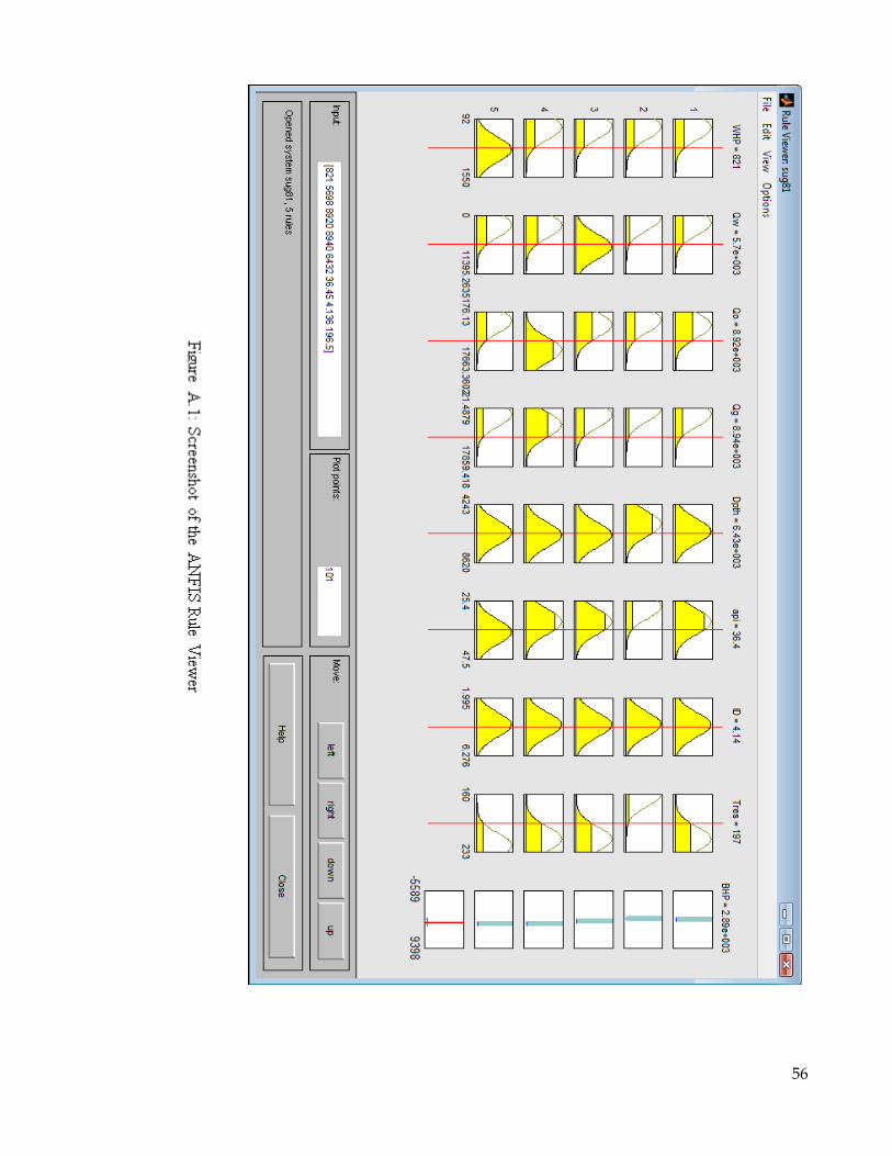
56
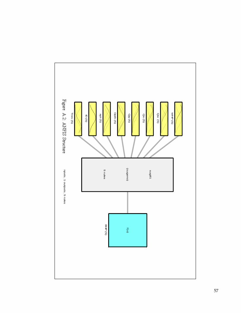
57
Syste
m s
ug81: 8
inputs
, 1 o
utp
uts
, 5 r
ule
s
WH
P (
5)
Qw
(5)
Qo (
5)
Qg (
5)
Dpth
(5)
api (
5)
ID (
5)
Tres (
5)
f(u)
BH
P (
5)
sug81
(sugeno)
5 r
ule
s

58
APPENDIX B
DATA AND NUMERIC RESULTS

59
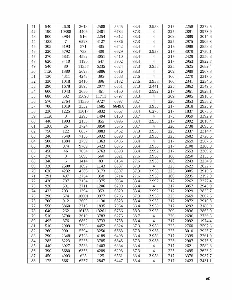
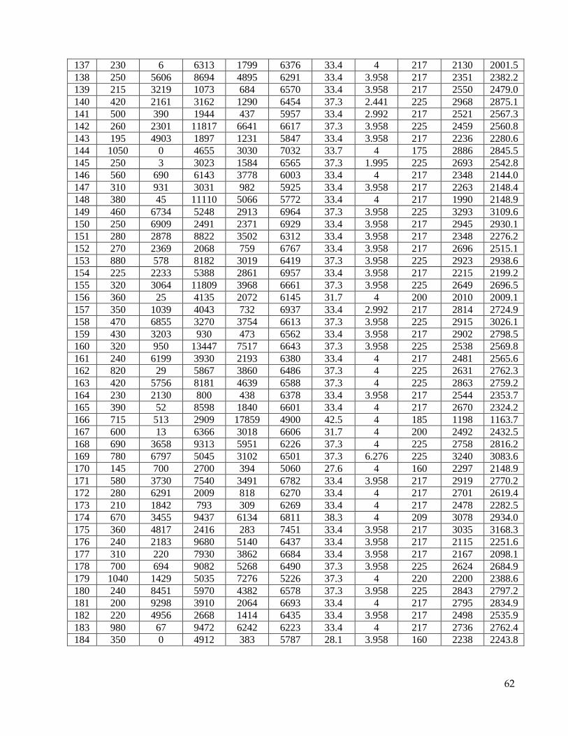
APPENDIX B
Table B.1: Data Used for Training the ANFIS Model and the Predicted BHP
SN WHP Qw Qo Qg Depth API ID Tres BHP Pred
BHP
1 670 3822 1848 248 6858 33.4 4 217 3234 3204.1
2 600 2420 824 1078 6567 31.7 3.958 200 2649 2866.7
3 340 140 5469 2620 6252 33.4 4 217 1851 1961.3
4 280 2245 6455 3118 6164 33.4 3.958 217 1975 2040.7
5 380 2758 3642 1344 6486 33.4 3.958 217 2383 2532.1
6 200 165 14790 7040 6584 37.3 3.958 225 2648 2423.6
7 225 1544 4218 1523 6135 33.4 3.958 217 1952 2077.5
8 390 2073 324 382 6811 31.7 2.992 200 2685 2818.7
9 1200 4 4106 3219 6846 38.3 4 209 3049 3071.2
10 220 806 7500 3750 6716 33.4 4 217 1906 2014.6
11 390 5521 6456 833 5944 33.4 4 217 2414 2447.3
12 210 746 4229 249 6026 27.6 3.958 160 2306 2182.7
13 295 3619 584 249 6808 33.4 4 217 3025 2759.0
14 460 1175 4315 1821 5998 33.4 4 217 2436 2276.8
15 280 6163 4178 2273 6542 33.4 4 217 2635 2668.9
16 850 396 1170 1043 6758 38.3 2.992 209 3135 2968.5
17 700 2102 6338 2580 6200 33.4 3.958 217 3039 2723.5
18 220 9481 4319 3170 5901 33.4 3.958 217 2344 2477.2
19 240 9 4438 1771 5664 31.7 4 200 1865 1786.7
20 300 7773 8091 5210 6683 37.3 3.958 225 3026 2806.7
21 220 3012 1391 771 5885 33.4 3.958 217 2222 2229.3
22 400 30 15094 7970 6889 33.4 3.958 217 2812 2555.6
23 580 1699 5017 2192 6530 37.3 3.958 225 2969 2758.7
24 400 10335 6552 5392 6583 37.3 6.276 225 2872 2899.7
25 250 329 16971 10454 6607 37.3 4 225 2599 2523.8
26 92 0 639 42 5146 26.2 3.958 160 1916 2004.2
27 270 2060 2314 1641 7025 31.7 2.992 200 2515 2538.5
28 340 126 3018 235 5687 28.1 4 160 2195 2299.3
29 220 3670 3730 1264 6394 33.4 4 217 2532 2397.0
30 1000 90 5910 3700 6535 37.3 4 225 2968 2986.2
31 900 719 2625 1299 6243 33.4 4 217 2944 2961.9
32 240 432 13083 5809 6310 33.4 3.958 217 2239 2259.4
33 240 2744 2165 983 6694 37.3 3.92 225 2580 2623.1
34 760 30 15170 7979 6717 37.3 3.958 225 3080 2966.1
35 225 3556 10612 5094 6248 33.4 4 217 2335 2347.6
36 300 1022 1434 610 6559 31.7 3.958 200 2531 2367.2
37 320 0 1929 253 6161 27.6 4 160 2206 2248.6
38 215 720 10187 5440 6759 33.4 3.958 217 2183 2235.2
39 400 1429 8927 4499 5533 33.4 3.958 217 2103 2043.5
40 230 1899 1256 417 6383 33.4 2.441 217 2761 2581.8
60
41 540 2628 2618 2508 5545 33.4 3.958 217 2258 2272.5
42 190 10380 4406 2481 6784 37.3 4 225 2891 2973.9
43 800 3984 916 2254 6312 38.3 4 209 2889 3014.6
44 1000 7 6593 4127 6386 37.3 4 225 2975 2906.3
45 305 5193 571 405 6742 33.4 4 217 3088 2853.8
46 220 5792 753 409 6629 33.4 3.958 217 3079 2750.1
47 270 5831 4582 3051 6410 33.4 4 217 2429 2556.8
48 620 3410 1190 547 5902 33.4 4 217 2953 2822.7
49 540 80 11357 6235 6824 37.3 3.958 225 2625 2682.4
50 1120 1380 5698 5886 6516 38.3 4 209 2989 2967.8
51 130 4311 4243 395 5588 27.6 4 160 2270 2317.5
52 330 1018 3410 396 5132 27.6 3.958 160 2341 2234.6
53 290 1678 3898 2077 6351 37.3 2.441 225 2862 2549.5
54 600 1043 3656 461 6150 33.4 2.992 217 2961 2828.1
55 680 502 15698 11711 6797 38.3 4 209 2905 2918.5
56 570 2764 11336 9727 6897 38.7 4 220 2853 2938.2
57 700 1019 3532 1685 6649.8 33.4 3.958 217 2818 2925.9
58 230 1225 13017 5832 6567 33.4 6.276 217 1837 2073.5
59 1120 0 2295 1494 8150 33.7 4 175 3059 3392.9
60 440 1903 2155 855 6995 33.4 3.958 217 2992 2816.4
61 1260 26 3724 3850 5676 38.7 4 220 2738 2693.6
62 750 122 6637 3883 5462 37.3 3.958 225 2337 2314.4
63 240 7549 7138 5032 6593 37.3 3.958 225 2682 2726.6
64 500 1384 2759 1363 6435 33.4 4 217 2659 2587.6
65 300 874 9789 5423 6375 33.4 3.958 217 2108 2200.8
66 450 46 7654 5763 6698 33.4 2.992 217 2553 2309.2
67 276 0 5890 560 5821 27.6 3.958 160 2250 2153.6
68 340 6 1414 83 6164 27.6 3.958 160 2243 2234.9
69 320 2508 1892 1143 6587 37.3 4 225 2622 2622.7
70 620 4232 4566 3173 6507 37.3 3.958 225 3085 2915.6
71 291 497 2754 358 5714 27.6 3.958 160 2235 2192.0
72 420 707 3154 1375 5964 33.4 2.992 217 2262 2377.4
73 920 501 2711 1206 6200 33.4 4 217 3057 2943.9
74 433 2031 1394 353 6520 33.4 2.992 217 2929 2833.7
75 290 674 16601 9977 6706 37.3 3.958 225 2669 2607.6
76 700 912 2609 1130 6523 33.4 3.958 217 2872 2910.8
77 550 5860 3715 1835 7064 33.4 3.958 217 3292 3180.0
78 640 262 16133 13261 6756 38.3 3.958 209 2836 2863.9
79 510 5790 3610 3783 6276 38.7 4 220 2696 2736.3
80 495 376 6862 3733 5758 33.4 4 217 2092 1974.4
81 510 2909 7298 4452 6624 37.3 3.958 225 2760 2597.3
82 260 9901 5594 3250 6663 37.3 3.958 225 3010 2925.7
83 290 2348 8728 4189 6498 33.4 3.958 217 2339 2261.0
84 285 8223 5235 3785 6845 37.3 3.958 225 2907 2975.6
85 440 3027 2538 1403 6334 33.4 4 217 2621 2582.8
86 390 5680 6353 4289 6293 37.3 4 225 2495 2623.2
87 450 4903 625 125 6561 33.4 3.958 217 3376 2937.7
88 175 5661 6257 2847 6447 33.4 4 217 2423 2431.1

61
89 260 3482 12344 7196 6753 37.3 3.958 225 2648 2698.2
90 850 2362 2198 413 6223 33.4 4 217 3418 3127.0
91 860 1883 2921 1972 6379 37.3 4 225 3007 3048.9
92 730 161 6260 4901 6126 33.4 4 217 2492 2352.7
93 630 1249 6277 4205 6758 37.3 3.958 225 2533 2651.0
94 260 6 5689 2583 6525 31.7 2.992 200 2224 2081.3
95 390 1156 3379 865 4885 28.1 3.958 160 2205 2230.1
96 740 1465 10258 6267 6595 37.3 3.958 225 2848 2869.6
97 990 238 2562 2175 6730 37.3 3.958 225 2921 3089.8
98 260 2472 16994 11250 6752 37.3 6.276 225 2373 2437.8
99 200 97 4731 1438 6612 31.7 3.958 200 2319 2057.3
100 490 5009 4737 5840 6891 38.3 3.958 209 2580 2732.7
101 200 1142 2256 792 6555 33.4 4 217 2242 2214.2
102 280 4506 1814 999 5975 33.4 3.958 217 2679 2410.3
103 570 7678 4766 6129 6781 38.3 4 209 2984 2932.6
104 300 1825 10846 4968 6448 33.4 3.958 217 2309 2363.8
105 250 1605 13395 6698 6693 33.4 3.958 217 2558 2452.3
106 1080 1833 1153 611 6571 31.7 4 200 3491 3246.6
107 390 1331 1891 1061 6772 33.4 3.958 217 2581 2566.4
108 580 937 4389 2717 5089 37.3 4 225 2177 2130.4
109 220 3065 2830 968 6146 33.4 3.958 217 2533 2299.1
110 960 47 9353 9353 6863 38.7 3.958 220 2766 2988.8
111 265 4623 1962 918 6908 31.7 3.958 200 2892 2614.7
112 205 318 1734 799 6214 33.4 1.995 217 2367 2379.0
113 342 0 6349 622 5625 27.6 4 160 2143 2234.9
114 610 500 3319 2323 6360 33.4 4 217 2438 2553.8
115 400 233 2220 313 5083 27.6 4 160 2284 2293.9
116 170 3646 7078 2980 6576.14 33.4 3.958 217 2378 2264.3
117 225 21 10727 4677 6113 33.4 3.958 217 2099 2071.6
118 747 204 3190 2871 4600 42.5 4 185 1827 2026.1
119 310 5935 12497 7336 6683 37.3 3.958 225 2774 2872.4
120 220 262 8468 1804 4770 25.4 3.958 160 1907 1842.5
121 230 81 2051 250 6322 35.3 2.441 233 2323 2461.3
122 580 5787 6713 5786 6645 38.7 3.958 220 2683 2879.0
123 425 145 3145 811 4688 25.4 4 160 2022 2122.3
124 245 5012 12095 9639 6587.1 37.3 3.958 225 2745 2739.5
125 250 61 12099 5178 6180 31 4 225 2301 2131.3
126 265 0 1870 168 5000 26.4 3.958 160 2092 2109.9
127 550 1347 5006 3504 6313 33.4 4 217 2546 2311.2
128 280 26 12869 5251 6666 33.4 4 217 2312 2336.2
129 180 2218 2097 1292 6085 33.4 2.441 217 2350 2326.3
130 480 2748 1692 1116 7296 33.4 4 217 2730 3048.4
131 220 1082 12617 4820 6623 33.4 3.958 217 2290 2351.0
132 570 2979 8221 6396 6746 38.3 3.958 209 2771 2704.3
133 730 3235 2950 1092 6325 37.3 4 225 3004 3100.3
134 540 1208 792 257 6532 33.4 3.958 217 2984 2809.2
135 365 0 2357 193 5126 26.4 3.958 160 2192 2172.2
136 225 9077 4331 2655 6676 33.4 3.958 217 2742 2833.1
62
137 230 6 6313 1799 6376 33.4 4 217 2130 2001.5
138 250 5606 8694 4895 6291 33.4 3.958 217 2351 2382.2
139 215 3219 1073 684 6570 33.4 3.958 217 2550 2479.0
140 420 2161 3162 1290 6454 37.3 2.441 225 2968 2875.1
141 500 390 1944 437 5957 33.4 2.992 217 2521 2567.3
142 260 2301 11817 6641 6617 37.3 3.958 225 2459 2560.8
143 195 4903 1897 1231 5847 33.4 3.958 217 2236 2280.6
144 1050 0 4655 3030 7032 33.7 4 175 2886 2845.5
145 250 3 3023 1584 6565 37.3 1.995 225 2693 2542.8
146 560 690 6143 3778 6003 33.4 4 217 2348 2144.0
147 310 931 3031 982 5925 33.4 3.958 217 2263 2148.4
148 380 45 11110 5066 5772 33.4 4 217 1990 2148.9
149 460 6734 5248 2913 6964 37.3 3.958 225 3293 3109.6
150 250 6909 2491 2371 6929 33.4 3.958 217 2945 2930.1
151 280 2878 8822 3502 6312 33.4 3.958 217 2348 2276.2
152 270 2369 2068 759 6767 33.4 3.958 217 2696 2515.1
153 880 578 8182 3019 6419 37.3 3.958 225 2923 2938.6
154 225 2233 5388 2861 6957 33.4 3.958 217 2215 2199.2
155 320 3064 11809 3968 6661 37.3 3.958 225 2649 2696.5
156 360 25 4135 2072 6145 31.7 4 200 2010 2009.1
157 350 1039 4043 732 6937 33.4 2.992 217 2814 2724.9
158 470 6855 3270 3754 6613 37.3 3.958 225 2915 3026.1
159 430 3203 930 473 6562 33.4 3.958 217 2902 2798.5
160 320 950 13447 7517 6643 37.3 3.958 225 2538 2569.8
161 240 6199 3930 2193 6380 33.4 4 217 2481 2565.6
162 820 29 5867 3860 6486 37.3 4 225 2631 2762.3
163 420 5756 8181 4639 6588 37.3 4 225 2863 2759.2
164 230 2130 800 438 6378 33.4 3.958 217 2544 2353.7
165 390 52 8598 1840 6601 33.4 4 217 2670 2324.2
166 715 513 2909 17859 4900 42.5 4 185 1198 1163.7
167 600 13 6366 3018 6606 31.7 4 200 2492 2432.5
168 690 3658 9313 5951 6226 37.3 4 225 2758 2816.2
169 780 6797 5045 3102 6501 37.3 6.276 225 3240 3083.6
170 145 700 2700 394 5060 27.6 4 160 2297 2148.9
171 580 3730 7540 3491 6782 33.4 3.958 217 2919 2770.2
172 280 6291 2009 818 6270 33.4 4 217 2701 2619.4
173 210 1842 793 309 6269 33.4 4 217 2478 2282.5
174 670 3455 9437 6134 6811 38.3 4 209 3078 2934.0
175 360 4817 2416 283 7451 33.4 3.958 217 3035 3168.3
176 240 2183 9680 5140 6437 33.4 3.958 217 2115 2251.6
177 310 220 7930 3862 6684 33.4 3.958 217 2167 2098.1
178 700 694 9082 5268 6490 37.3 3.958 225 2624 2684.9
179 1040 1429 5035 7276 5226 37.3 4 220 2200 2388.6
180 240 8451 5970 4382 6578 37.3 3.958 225 2843 2797.2
181 200 9298 3910 2064 6693 33.4 4 217 2795 2834.9
182 220 4956 2668 1414 6435 33.4 3.958 217 2498 2535.9
183 980 67 9472 6242 6223 33.4 4 217 2736 2762.4
184 350 0 4912 383 5787 28.1 3.958 160 2238 2243.8
63
185 820 1645 11727 6004 6399 37.3 6.276 225 2789 2694.0
186 180 2896 4806 476 5860 27.6 4 160 2117 2278.2
187 410 0 2718 457 4948 26.4 4 160 2190 2209.7
188 275 3707 6534 4071 6712 37.3 4 225 2358 2461.8
189 450 2118 6355 3902 6425 37.3 3.958 225 2334 2378.3
190 270 153 16848 9283 6214 37.3 3.958 225 2477 2447.4
191 230 1219 5265 2643 6348 33.4 3.958 217 1732 1936.2
192 210 1986 2655 1232 6646 31.7 4 200 1996 2250.7
193 230 327 7657 3178 6859 31.7 3.958 200 1845 2043.2
194 180 1065 5200 2226 6776 33.4 3.958 217 1811 2042.0
195 225 1390 5073 2379 6331 33.4 4 217 1751 1974.4
196 270 1083 6600 2844 5422 33.4 6.276 217 1421 1474.1
197 250 1829 11426 6410 6778 33.4 3.958 217 2262 2420.1
198 600 4448 1730 1114 6874 33.4 3.958 217 3141 3181.6
199 790 633 11785 648 6224 37.3 4 225 2903 2921.8
200 440 4179 1816 1778 6834 33.4 3.958 217 2537 2870.8
201 290 80 7900 4005 6442 31.7 4 200 1941 1933.4
202 240 6182 748 555 6832 37.3 4 225 3006 2955.1
203 580 42 4658 1779 5841 33.4 4 217 2266 2329.4
204 230 1022 1488 731 6298 33.4 4 217 2191 2170.5
205 750 2791 1383 524 6509 33.4 4 217 3180 3169.8
206 205 4970 926 535 6407 33.4 4 217 2646 2578.2
207 293 47 5164 537 6050 26.4 3.958 160 2079 2105.0
208 1030 175 3064 199 5071 37.3 4 225 2634 2570.4
209 295 13 12727 5015 6532 33.4 3.958 217 2282 2320.2
210 120 5006 939 82 5006 27.6 4 160 2336 2361.7
211 230 1859 9013 4669 6494 33.4 3.958 217 1996 2178.9
212 340 1628 6762 3483 6581 31.7 4 200 2230 2108.0
213 800 536 8106 4434 6429 37.3 3.958 225 3016 2753.0
214 550 259 15941 12163 6816 38.7 4 220 2800 2829.0
215 250 28 13833 3140 6293 37.3 3.958 225 2495 2385.7
216 730 3505 1715 1216 6606 33.4 4 217 3342 3195.0
217 500 1022 8618 4344 6778 37.3 3.958 225 2510 2569.8
218 220 182 6078 2924 6508 31.7 2.992 200 2159 2011.6
219 495 844 5746 2896 6064 33.4 4 217 2234 2173.5
220 370 2700 7012 1262 6110 31.7 3.958 200 2539 2395.9
221 195 1095 6155 3508 6388 33.4 3.958 217 2012 1820.0
222 320 1611 1954 344 6613 37.3 4 225 2938 2672.2
223 260 13 12893 6240 5871 33.4 4 217 2047 2132.0
224 290 7 6593 3191 6403 31.7 4 200 1950 1882.7
225 420 6664 2047 1101 6273 33.4 4 217 2798 2767.3
226 480 2789 7280 976 6054 33.4 4 217 2601 2592.1
227 760 518 4883 2461 6570 37.3 3.958 225 2714 2878.1
228 230 2452 745 107 6459 33.4 2.992 217 2788 2605.7
229 290 4288 3712 3203 6881 37.3 4 225 2940 2711.1
230 240 8124 4690 3452 6729 37.3 3.958 225 2962 2889.1
231 349 1064 1664 158 6223 27.6 4 160 2325 2327.2
232 190 2678 8344 4013 6434 33.4 4 217 2118 2140.9

64
233 660 3121 479 1520 6656 38.3 2.992 209 3026 3076.0
234 210 3604 3984 1801 6340 33.4 3.958 217 2289 2303.4
235 415 34 5624 731 5838 35.3 4 233 2202 2280.5
236 600 1479 772 49 6541 33.4 4 217 3100 2928.5
237 400 1466 5198 1429 6678 33.4 4 217 2557 2491.4
238 250 7857 4878 2614 6429 33.4 3.958 217 2562 2658.3
239 225 7665 2735 1939 6742 33.4 4 217 3029 2842.6
240 700 1070 720 515 6565 33.4 3.958 217 2941 2971.8
241 550 1082 968 613 6800 33.4 3.958 217 3155 2880.5
242 320 65 7134 2575 5944 33.4 4 217 1960 1930.4
243 110 1993 2526 248 5750 27.6 4 160 2326 2211.4
244 880 412 2936 2508 6223 38.1 4 207 2733 2694.3
245 210 2496 8037 3416 6341 33.4 4 217 2141 2123.5
246 940 142 11693 6373 6472 37.3 3.958 225 2926 2987.9
247 1000 13 3284 1419 6350 33.4 4 217 2853 3006.8
248 260 1688 1602 107 4946 27.6 3.958 160 2312 2250.8
249 200 2719 2180 1049 6656 33.4 2.992 217 2497 2521.8
250 255 4311 3020 1386 6251 33.4 3.958 217 2385 2435.4
251 300 1833 9344 4289 6462 33.4 4 217 2136 2266.1
252 640 1454 1550 419 6603 33.4 3.958 217 3358 2974.4
253 260 240 6086 2191 5925 33.4 4 217 1841 1872.1
254 220 1511 3964 1708 6788 33.4 3.958 217 2251 2207.6
255 300 103 11341 5058 5550 33.4 4 217 2039 2038.7
256 190 2698 4168 2613 6525 31.7 4 200 2094 2052.5
257 250 3916 3688 1682 6656 33.4 4 217 2498 2511.7
258 225 2283 10544 4766 6022 33.4 4 217 2051 2201.4
259 440 1816 3542 1325 6054 33.4 4 217 2344 2395.6
260 245 2936 6384 3633 6715 31.7 3.958 200 2235 2134.1
261 230 2422 5029 2419 6643 33.4 3.958 217 2185 2189.8
262 340 861 10032 5217 6394 33.4 3.958 217 2098 2262.2
263 1050 299 3388 1843 5570 33.4 4 217 2698 2749.2
264 450 21 2268 229 6026 33.4 3.958 217 2408 2408.0
265 230 4147 1694 960 6109 33.4 2.992 217 2489 2492.9
266 250 2276 11110 5900 6729 37.3 3.958 225 2560 2548.5
267 320 1948 1693 907 6076 33.4 2.992 217 2258 2443.1
268 290 23 7489 3565 6583 31.7 4 200 2056 1960.3
269 720 558 2379 2025 6775 37.3 4 225 2590 2927.8
270 250 2075 8844 3600 6538 33.4 3.958 217 2211 2242.0
271 330 2036 3436 268 4912 37.3 4 225 2352 2338.1
272 230 538 5379 2345 6719 33.4 4 217 2095 2017.1
273 690 939 2321 1068 6449 33.4 3.958 217 2674 2875.5
274 350 15 7600 980 6170 33.4 6.276 217 2241 1974.5
275 240 4902 4011 1785 6332 33.4 4 217 2405 2460.1
276 680 2623 3577 644 6744 33.4 3.958 217 3522 3168.8
277 225 6828 7457 3274 6530 33.4 6.276 217 2456 2420.8
278 950 1910 5729 10840 6979 38.3 4 209 3236 2818.0
279 240 5641 6412 3488 6033 33.4 3.958 217 2240 2291.1
280 1120 2030 2243 357 6481 33.4 4 217 3374 3374.2

65
281 1170 426 4200 357 6465 37.3 4 225 3181 3219.1
282 320 3849 6306 3090 6380 31.7 3.958 200 2375 2235.6
283 450 20 4991 654 6046 33.4 4 217 2332 2368.8
284 950 84 16739 2628 6776 37.3 6.276 225 2838 2925.3
285 650 40 3911 1877 5512 33.4 4 217 2128 2301.4
286 780 285 3203 1794 6160 33.4 2.992 217 3027 2826.9
287 540 1018 5467 2515 5830 33.4 4 217 2202 2238.2
288 840 3189 686 1520 6362 38.7 4 220 2926 3095.9
289 230 4220 3880 1932 6849 33.4 4 217 2360 2590.2
290 435 2498 1751 756 6328 33.4 4 217 2597 2621.4
291 235 42 3793 1547 6595 31.7 2.441 200 2271 2296.6
292 700 1683 2323 1445 6453 37.3 3.958 225 2718 2941.9
293 240 0 1150 135 5556 27.6 4 160 2266 2207.2
294 345 3956 5160 2585 6773 33.4 3.958 217 2572 2578.9
295 220 4097 7316 3716 6515 33.4 3.958 217 2234 2305.1
296 580 1087 2196 1272 6581 37.3 3.958 225 2555 2814.7
297 950 2054 2746 1329 6548 38.3 4 209 3041 3099.1
298 410 1706 1594 558 6200 31.7 2.992 200 2389 2593.2
299 240 2797 1154 345 6385 37.3 3.958 225 2387 2612.8
300 200 2435 5549 2908 6790 33.4 3.958 217 2049 2146.9
301 425 125 6475 3179 6616 31.7 6.276 200 2078 1947.6
302 430 1402 5439 1985 6688 33.4 3.958 217 2349 2456.2
303 348 749 5387 1848 6555 33.4 4 217 2098 2241.4
304 640 6087 2609 2335 6816 38.3 4 209 3007 3022.8
305 260 5143 2499 1234 6376 33.4 4 217 2322 2569.4
306 270 4513 2495 1285 6493 33.4 3.958 217 2319 2581.7
307 200 565 6675 2383 5888 33.4 3.958 217 2039 1837.1
308 550 241 4315 1765 6595 31.7 2.992 200 2379 2658.3
309 245 69 8559 916 6012 33.4 4 217 1989 2128.8
310 250 1198 719 167 5658 31.7 2.992 200 2140 2239.2
311 360 12 4048 1688 5996 33.4 3.958 217 1836 2043.1
312 610 695 3705 1482 6290 31.7 3.958 200 2337 2594.4
313 680 1745 603 522 6812 37.3 3.958 225 2990 3110.2
314 320 1953 5023 2511 6124 31.7 4 200 1968 2056.5
315 200 3160 5544 2201 6173 33.4 3.958 217 1995 2151.5
316 320 2081 4421 1998 6804 33.4 3.958 217 2249 2376.1
317 440 1772 4058 1554 6350 33.4 3.958 217 2273 2460.2
318 260 4544 1115 827 6517 33.4 3.958 217 2374 2634.9
319 650 4007 6483 3241 5995 33.4 4 217 2367 2612.2
320 280 3312 1320 665 6468 33.4 3.958 217 2441 2536.3
321 440 1353 6847 2143 6134 33.4 4 217 2125 2286.4
322 998 466 2276 2208 4750 42.5 4 185 1920 1992.8
323 170 2944 4379 2128 6651 33.4 3.958 217 2035 2234.2
324 230 371 15080 8143 6723 31.7 6.276 200 1929 2002.8
325 180 2748 3826 1990 6626 31.7 4 200 2166 2168.5
326 1550 235 4373 669 6788 33.4 4 217 3604 3555.6
327 210 954 3288 1335 6689 31.7 2.992 200 2213 2313.5
328 160 98 10817 714 4983 27.6 4 160 2103 2141.7
66
329 215 399 4585 2095 6254 31.7 2.992 200 1944 2038.3
330 410 2059 5018 1882 6121 33.4 4 217 2107 2311.1
331 230 409 5603 2605 6449 31.7 4 200 1767 1892.7
332 400 57 4343 2267 6423 31.7 3.958 200 1900 2136.8
333 190 1939 3418 1883 6602 33.4 3.958 217 1885 2123.5
334 260 2854 4408 2032 5608 31.7 4 200 1810 1985.3
335 200 819 2296 790 6557 33.4 4 217 1933 2183.9
336 220 259 5034 1953 6367 33.4 3.958 217 1748 1946.2
337 185 586 7336 2964 6640 31.7 3.958 200 1753 1959.8
338 280 6130 2348 1649 5859 33.4 3.958 217 2283 2408.2
339 820 1448 743 999 6962 38.3 4 209 3020 3087.3
340 300 1625 966 365 7033 33.4 1.995 217 3153 2949.6
341 220 2301 3645 1903 5889 33.4 4 217 2059 1995.6
342 340 475 1746 461 6312 33.4 3.958 217 2335 2344.7
343 225 1893 14151 9170 6466 37.3 3.958 225 2587 2528.4
344 975 391 4493 4143 4700 42.5 3.958 185 2122 1974.9
345 550 1253 2442 2086 6639 38.3 2.441 209 2997 2858.7
346 810 3436 11246 1844 6463 37.3 4 225 2946 3165.1
347 240 66 16488 8706 6629 33.4 3.958 217 2684 2384.5
348 560 3484 4208 2503 6593 37.3 3.958 225 2636 2869.5
349 350 3746 1820 1578 6672 33.4 4 217 2472 2642.1
350 550 2366 1063 461 6275 33.4 3.958 217 2763 2805.7
351 210 2922 938 315 6644 33.4 4 217 2634 2510.5
352 310 1455 1545 593 6149 33.4 2.992 217 2268 2458.5
353 200 1089 2718 1163 6386 33.4 2.441 217 2476 2363.3
354 370 8187 8024 3547 6859 37.3 4 225 2937 2957.3
355 383 0 836 145 5858 26.4 4 160 2192 2232.7
356 1020 673 2887 1969 6041 33.4 2.992 217 2994 2990.6
357 250 3623 1729 832 6369 33.4 3.958 217 2466 2473.8
358 800 672 6556 5009 5628 37.6 4 196 2523 2332.6
359 450 27 2674 289 6329 33.4 4 217 2789 2502.6
360 320 1112 6890 3286 6453 31.7 3.958 200 2166 2039.8
361 380 9222 9637 7363 6337 37.3 3.958 225 2783 2754.7
362 260 4112 7536 3791 6486 37.3 4 225 2612 2460.1
363 680 452 853 298 6642 33.4 4 217 2920 2934.4
364 190 1734 6008 2481 6622 33.4 3.958 217 2169 2077.7
365 245 174 1002 359 6442 33.4 3.958 217 2340 2225.2
366 250 7528 3272 1594 6433 33.4 3.958 217 2611 2690.1
367 195 16 2032 175 6094 35.3 1.995 233 2260 2438.0
368 290 4047 3297 1039 6267 31.7 4 200 2502 2362.3
369 135 32 2080 189 6399 27.6 4 160 2190 2148.4
370 320 1242 10589 4680 6493 33.4 3.958 217 2259 2336.8
371 310 1311 3851 2268 6483 31.7 4 200 2184 2109.4
372 210 3708 3354 1452 6675 31.7 6.276 200 2421 2169.0
373 230 4769 10614 5424 6896 33.4 4 217 2895 2598.4
374 190 3797 7051 4146 6863 37.3 3.958 225 2571 2465.6
375 200 4537 2214 1050 5923 33.4 4 217 2221 2297.9
376 280 6185 7468 3809 6573 33.4 3.958 217 2492 2587.1
67
377 250 2811 9149 3605 6297 33.4 3.958 217 2251 2258.9
378 650 1037 2095 1067 5899 33.4 3.958 217 2456 2620.5
379 1033 500 4500 4640 4660 42.5 4 185 2098 1946.3
380 360 1261 5339 2435 6599 31.7 4 200 2058 2205.8
381 495 3014 6174 2877 6296 33.4 4 217 2776 2448.8
382 420 41 3099 381 5917 27.6 3.958 160 2190 2251.3
383 780 4218 5801 1265 6526 33.4 3.958 217 3185 3220.6
384 225 865 3234 58 6500 27.6 4 160 2336 2270.4
385 1100 19 4673 4281 5992 37.3 4 225 2909 2793.6
386 180 6763 4604 2412 6840 33.4 4 217 2833 2742.3
387 460 1179 7821 3410 5824 33.4 4 217 2180 2114.8
388 300 2003 11715 5190 6541 33.4 4 217 2402 2434.8
389 400 4121 7619 3551 5985 33.4 6.276 217 2425 2101.2
390 740 4823 4277 3866 5905 38.1 4 207 2788 2675.9
391 120 0 2043 282 5249 27.6 3.958 160 2011 2067.2
392 180 848 5833 2677 6027 33.4 2.992 217 2220 1945.7
393 280 3852 3335 1614 6438 37.3 4 225 2686 2597.6
394 390 1282 14944 9056 6693 37.3 3.958 225 2765 2705.9
395 900 182 1118 807 8620 47.5 2.992 189 3524 3289.1
396 590 1143 11277 5943 6392 37.3 6.276 225 2542 2418.4
397 600 2480 15620 12481 6458 38.7 4 220 2691 2956.7
398 145 666 1120 166 6173 27.6 4 160 2204 2178.1
399 250 3567 17663 11587 6645 37.3 6.276 225 2612 2503.9
400 700 1458 9423 4881 7038 37.3 3.958 225 3065 2921.2
401 560 1189 723 310 6700 33.4 6.276 217 3048 2802.7
402 330 331 7022 3223 6240 31.7 4 200 2050 1936.8
403 320 854 176 21 6350 33.4 2.441 217 2903 2636.2
404 320 5495 9437 5813 6913 37.3 3.958 225 3015 2796.0
405 305 9563 3700 1443 6712 37.3 3.958 225 3076 3019.9
406 240 2484 5328 2461 6195 33.4 3.958 217 1889 2078.0
407 470 16 5284 2198 6017 31.7 4 200 1899 2127.4
408 1028 275 3658 2977 4800 42.5 3.958 185 1874 2008.6
409 280 782 6457 2551 6696 31.7 3.958 200 1965 2099.7
410 196 1917 4955 1823 6093 33.4 4 217 1796 2030.1
411 205 335 4260 1286 6013 31.7 3.958 200 2038 1957.9
412 180 3018 4781 2271 6580 33.4 6.276 217 1880 1999.3
413 300 2353 4388 2111 6058 33.4 3.958 217 2131 2129.3
414 532 3084 10503 3812 6165 33.4 4 217 2482 2592.1
415 600 4404 3309 1995 6868 37.6 4 196 2607 2922.9
416 570 16 7868 2392 5993 33.4 4 217 2327 2308.6
417 260 13 12846 5485 6478 31.7 3.958 200 2146 2190.7
418 620 294 2506 561 6576 33.4 4 217 2640 2821.0
419 460 4250 3207 2854 6679 38.3 2.992 209 2855 2822.8
420 220 5707 9802 6253 6495.99 37.3 3.958 225 2745 2570.1
421 250 4353 8565 3854 5899 33.4 3.958 217 2135 2185.5
422 870 1345 4882 2168 6441 33.4 4 217 2858 3046.4
423 210 3251 2177 1027 6555 33.4 4 217 2370 2423.0
424 360 375 5585 2915 6551 33.4 4 217 2131 2060.9
68
425 220 7774 8288 5512 6669.36 37.3 3.958 225 2895 2724.5
426 1000 194 4121 437 6132 33.4 4 217 2854 3004.2
427 220 6956 7971 6154 6754 37.3 4 225 2800 2734.8
428 230 1042 8098 3320 6047 33.4 4 217 1906 1952.2
429 390 842 8112 1063 4243 35.3 4 233 2014 1955.3
430 260 3173 6442 3369 5671 33.4 4 217 1927 1937.7
431 200 1218 6957 3388 6680 31.7 3.958 200 2030 1970.9
432 210 11395 5437 3969 6264 33.4 3.958 217 2970 2704.7
433 210 1278 9934 4033 6574 33.4 3.958 217 2138 2222.5
434 917 381 1435 1673 4700 42.5 4 185 1966 1964.3
435 210 1501 7542 3658 6372 33.4 4 217 1932 1980.2
436 230 1588 13390 6561 6649 31.7 6.276 200 2182 2040.6
437 280 48 9522 2819 6340 31 4 225 2220 2048.7
438 530 59 9787 2995 6621 33.4 4 217 2496 2465.2
439 560 4910 2195 1328 6653 37.3 6.276 225 3045 2967.0
440 185 3938 3563 2636 6248 33.4 4 217 2025 2199.7
441 880 1976 7200 3435 6314 33.4 3.958 217 2855 2956.5
442 280 10715 275 239 7190 37.3 3.958 225 3206 3389.4
443 220 6197 3640 1867 5928 33.4 3.958 217 2189 2348.3
444 187 48 2360 210 4971 27.6 4 160 2195 2170.2
445 540 1444 5431 2216 6454 37.3 4 225 2495 2646.3
446 230 8755 7985 4639 6547 37.3 6.276 225 2424 2594.6
447 230 3591 5986 3370 6501 33.4 3.958 217 2183 2227.5
448 330 2 1758 621 6591 31.7 3.958 200 2200 2333.6
449 180 5690 5510 3174 6830 33.4 3.958 217 2322 2636.2
450 270 5133 5154 2896 6926 33.4 3.958 217 2575 2719.2
451 250 1206 10069 4984 6666 33.4 3.958 217 2143 2276.1
452 220 3887 1871 720 4912 33.4 2.992 217 2186 2125.5
453 200 36 3937 1917 6258 31.7 2.992 200 1864 2001.4
454 300 5703 5889 3569 6523 37.3 4 225 2580 2667.4
455 1025 657 4038 4001 6282 37.6 3.958 196 2761 2718.2
456 250 3402 3670 2573 6670 33.4 2.992 217 2541 2474.8
457 200 8026 1529 1622 6448 37.3 3.958 225 2805 2802.6
458 200 224 6576 736 5191 27.6 3.958 160 2159 2090.7
459 260 9896 7404 5257 6679 37.3 3.958 225 2895 2893.1
460 310 349 2446 575 5855 33.4 4 217 2257 2133.4
461 120 16 1043 83 6100 27.6 3.958 160 2031 2096.6
462 306 0 2404 221 6056 27.6 4 160 2202 2247.5
463 750 1021 4883 3052 6642 37.3 3.958 225 2819 2889.9
464 480 3267 5539 2814 7595 37.3 4 225 2953 3069.0
465 240 1468 12385 7059 6631 33.4 3.958 217 2325 2385.0
466 250 4 4096 1311 6589 31.7 4 200 2252 2113.9
467 425 0 4171 355 5732 27.6 4 160 2274 2311.4
468 720 3882 3361 1502 6500 33.4 3.958 217 3175 3129.9
469 255 773 10770 5105 6053 33.4 3.958 217 2095 2141.8
470 230 1282 450 324 6592 31.7 2.992 200 2617 2470.8
471 340 4878 690 351 6497 33.4 3.958 217 3045 2768.2
472 410 79 2401 146 5650 27.6 3.958 160 2271 2275.5

69
473 350 4082 4018 1924 6201 33.4 3.958 217 2608 2442.7
474 240 1512 12363 6367 6359 31.7 3.958 200 2273 2240.2
475 435 306 5694 478 5730 27.6 3.958 160 2287 2275.6
476 300 103 9284 2107 5215 28.1 3.958 160 1937 1984.6
477 260 5603 3478 1878 6649 33.4 3.958 217 2484 2689.4
478 290 4950 6300 3604 6589 37.3 4 225 2745 2613.7
479 200 829 6447 3249 6587 33.4 4 217 1924 1904.2
480 250 1424 746 285 5994 33.4 2.992 217 2279 2372.6
481 260 7712 8189 14854 6718 37.3 3.958 225 2939 2879.9
482 1050 1500 13503 6360 6827 31.7 3.958 200 3283 3134.1
483 990 659 4529 2183 5027 33.4 4 217 2417 2535.5
484 200 507 2873 1006 6020 35.3 4 233 2020 1988.7
485 650 5430 2316 1753 7000 38.3 4 209 3162 3145.1
486 320 7829 11550 6295 6874 37.3 4 225 2934 2860.1
487 840 966 1334 868 6672 33.7 4 175 2831 2735.1
488 275 3666 10434 5822 6856 33.4 3.958 217 2848 2550.6
489 245 539 9437 4700 5668 33.4 2.992 217 2228 2061.7
490 830 5214 2615 1577 6510 33.4 4 217 3089 3319.5
491 345 4220 4701 1241 6256 33.4 3.958 217 2506 2523.7
492 410 2921 10728 5235 5893 33.4 6.276 217 2178 2118.8
493 100 2996 333 184 6371 33.4 2.441 217 2615 2535.2
494 340 2043 3277 1416 6363 33.4 3.958 217 2306 2351.3
495 440 962 755 278 6076 33.4 4 217 2517 2472.3
496 620 3491 5648 2790 6587 37.3 3.958 225 2739 2912.7
497 310 4672 5528 2515 6639 33.4 3.958 217 2535 2579.9
498 220 43 8458 3942 6256 31.7 4 200 1726 1867.3
499 450 1196 6187 693 5897 33.4 4 217 2208 2433.9
500 280 648 2146 966 6773 31.7 2.441 200 2275 2546.4
501 320 7 7303 2826 6383 33.4 4 217 1899 2026.3
502 355 913 9831 3126 6831 33.4 3.958 217 2336 2408.6
503 210 1266 7465 3367 6522 33.4 4 217 1914 2015.6
504 760 193 10539 5891 6637 33.4 4 217 2440 2700.8
505 430 2150 1628 402 6263 33.4 3.958 217 2493 2617.9
506 285 1412 1511 364 6494 33.4 2.992 217 2385 2565.3
507 750 1947 4653 3187 6015 33.4 3.958 217 2717 2673.3
508 393 0 5603 986 5635 26.4 3.958 160 2198 2096.8
509 350 2036 13508 7146 6727 37.3 4 225 2651 2697.5
510 190 254 1576 561 6448 33.4 4 217 2116 2117.5
511 460 157 5083 579 5185 27.6 3.958 160 2256 2260.7
512 260 1181 13398 6391 6468 33.4 4 217 2349 2373.6
513 300 3468 13286 7414 6739 37.3 3.958 225 2735 2760.9
514 230 52 17284 8953 6326 33.4 3.958 217 2404 2324.9
515 780 286 7411 2794 6407 33.4 4 217 2906 2747.4
516 220 1930 7304 4083 6026 33.4 3.958 217 1970 1880.6
517 100 93 6567 722 5766 27.6 3.958 160 1984 2029.3
518 375 0 1943 295 5095 26.4 3.958 160 2216 2159.7
519 240 3576 8424 4296 6131 33.4 3.958 217 2243 2175.7
520 305 113 13999 7154 7006 33.4 3.958 217 2354 2474.9

70
521 310 1488 4326 1977 6267 33.4 4 217 2235 2130.8
522 150 26 3724 384 5922 27.6 3.958 160 2047 2088.5
523 235 5866 4425 2960 6831 33.4 3.958 217 2684 2735.8
524 295 155 4396 761 5930 26.4 4 160 2114 2118.9
525 340 4731 1654 1586 6848 33.4 4 217 2661 2831.7
526 400 0 4230 495 5050 26.4 4 160 2246 2209.5
527 290 2369 4897 2503 6544 37.3 3.958 225 2392 2386.7
528 470 107 2572 442 5250 27.6 3.958 160 2287 2267.4
529 680 3872 7652 6963 6985 38.3 3.958 209 2823 2895.2
530 240 1095 9855 4642 6235 33.4 4 217 2125 2131.4
531 360 2 1139 159 5066 27.6 3.958 160 2217 2225.9
532 250 5810 4678 2708 6456 37.3 3.958 225 2566 2642.5
533 480 1188 7060 826 6664 33.4 6.276 217 2689 2473.5
534 520 4978 5393 3748 6870.5 37.3 3.958 225 3033 2980.6
535 450 1956 3219 2163 6262 33.4 4 217 2577 2361.5
536 390 0 3044 286 6229 27.6 3.958 160 2267 2247.1
537 290 4206 7444 5501 5833 33.4 4 217 2025 2053.1
538 330 2623 4725 2343 5964 33.4 4 217 2291 2129.7
539 285 67 13287 5993 6516 33.4 4 217 2306 2320.1
540 400 134 6250 3106 6510 31.7 4 200 2303 2065.2
541 255 4657 4264 1748 6209 33.4 3.958 217 2507 2405.5
542 590 3046 1549 526 6769 37.3 4 225 3196 3140.0
543 420 0 2700 413 6060 26.4 3.958 160 2269 2181.8
544 220 1263 10656 5402 6828 33.4 3.958 217 2307 2326.3
545 100 1870 630 43 5907 27.6 4 160 2320 2217.7
546 170 4322 2441 1448 6741 33.4 2.992 217 2780 2649.5
547 280 2013 10115 4946 6256 33.4 3.958 217 2056 2265.4
548 480 2333 1690 809 6628 37.3 4 225 2641 2869.4
549 225 2129 2927 1098 6083 33.4 4 217 2071 2168.8
550 175 5593 7177 3538 6606 33.4 6.276 217 2183 2329.7
551 500 1259 4941 2693 6559 31.7 2.992 200 2511 2529.8
552 410 4 4367 1943 6075 33.4 3.958 217 1990 2105.5
553 250 1167 1865 675 5982 33.4 4 217 2056 2138.2
554 700 371 7321 3199 5963 33.4 4 217 2291 2430.3
555 200 7313 1726 1267 6783 31.7 3.958 200 2638 2602.6
556 520 3093 13271 7312 6642 37.3 6.276 225 2525 2619.8
557 940 1260 2240 1772 7122 33.7 4 175 2831 2929.9
558 255 4491 4787 2509 6244 33.4 3.958 217 2192 2350.6
559 570 1557 3338 2464 6194 37.6 3.958 196 2580 2573.5
560 240 2165 2835 1539 6815 31.7 3.958 200 2166 2311.4
561 340 33 8167 2687 6318 33.4 4 217 2000 2104.8
562 260 3524 6374 3181 6787 33.4 3.958 217 2194 2375.3
563 260 736 1663 715 6045 33.4 3.958 217 1864 2123.9
564 200 5 5311 1816 6828 31.7 3.958 200 2224 2047.0
565 280 1635 4704 1594 6240 33.4 3.958 217 2019 2179.4
566 1058 66 6567 5910 4770 42.5 4 185 2152 1997.9
567 205 415 13424 6511 6213 33.4 3.958 217 2145 2211.9
568 760 4488 4295 2925 6548 37.3 3.958 225 2919 3161.7

71
569 340 137 2917 300 5250 27.6 4 160 2232 2260.8
570 250 2303 1382 618 6709 37.3 2.992 225 2684 2772.3
571 230 2759 401 262 6517 33.4 2.441 217 2959 2707.2
572 310 1374 8878 8017 6733 31.7 4 200 1973 2177.7
573 315 210 2123 191 6000 27.6 4 160 2233 2264.6
574 150 103 4569 356 5593 27.6 3.958 160 2020 2100.0
575 540 443 2361 756 6055 33.4 4 217 2428 2508.6
576 220 5723 8477 4078 5815.8 33.4 3.958 217 2329 2160.4
577 300 3349 1316 505 6353 37.3 4 225 2804 2680.5
578 185 2025 819 405 6315 33.4 3.958 217 2520 2271.3
579 560 151 9264 3974 6334 37.3 3.958 225 2533 2500.5
580 340 772 5767 2699 6309 33.4 4 217 2316 2031.9
581 230 9031 6566 3986 6390 37.3 3.958 225 2542 2699.5
582 720 2661 9434 6736 6690 37.3 4 225 2917 2906.9
583 190 7317 1784 994 6254 33.4 4 217 2649 2582.9
584 365 4041 2073 1780 6502 33.4 4 217 2681 2606.2
585 680 1560 9501 5292 6356 37.3 4 225 2740 2715.0
586 930 2723 7037 4032 6501 37.3 3.958 225 3260 3144.2
587 900 2016 3522 4417 6980 38.3 3.958 209 2867 3080.9
588 285 1120 6011 2525 6440 33.4 3.958 217 2281 2070.6
589 140 148 10452 669 5651 27.6 3.958 160 2150 2092.2
590 1100 417 2400 463 6282 33.4 4 217 3293 3107.9
591 300 1717 11591 4660 5855 33.4 4 217 2213 2248.8
592 310 1001 8266 4464 5785 33.4 4 217 1950 1910.7
593 760 84 4855 1359 5434 33.4 2.992 217 2644 2568.6
594 1110 1100 1545 618 6874 33.4 4 217 3571 3393.5
595 250 1433 4254 1651 6424 31.7 2.992 200 2549 2293.8
596 230 211 8969 3552 6644 33.4 3.958 217 2096 2114.2
Table B.2: Data Used for Testing the ANFIS Model and the Predicted BHP
SN WHP Qw Qo Qg Depth API ID Tres BHP Pred.
BHP
1 280 1675 3195 230 5064 27.6 4 160 2300 2304.6
2 170 2246 9701 5190 6537 31.7 3.958 200 2230 2140.8
3 700 3738 1341 992 6415 33.4 4 217 3052 3111.5
4 260 3142 2275 1119 6548 33.4 2.992 217 2629 2592.5
5 190 24 12215 5631 6242 33.4 4 217 2049 2131.2
6 525 1040 14260 8099 7358 37.3 3.958 225 2810 2947.5
7 310 2550 13798 7810 6815 37.3 4 225 2679 2725.8
8 550 287 7481 4301 6054 33.4 4 217 2306 2135.4
9 396 488 2763 323 5755 26.4 3.958 160 2301 2201.0
10 960 45 7525 2709 6212 37.3 3.958 225 2950 2905.9
11 170 3530 7199 2757 6710 33.4 4 217 2460 2310.4

72
12 920 359 9910 8275 5986 38.7 4 220 2566 2781.7
13 280 10144 5156 2949 6700 33.4 3.958 217 2965 2919.4
14 510 1620 994 800 6189 33.4 4 217 2728 2607.9
15 350 2224 13546 6638 6593 37.3 3.958 225 2621 2689.8
16 336 834 5630 1115 4888 28.1 3.958 160 2174 2161.0
17 230 561 839 421 6370 33.4 3.958 217 2240 2203.3
18 930 2105 4495 4166 6186 38.7 3.958 220 2731 2895.7
19 320 442 14791 2026 6191 33.4 4 217 2726 2369.3
20 220 4852 796 426 6021 33.4 3.958 217 2690 2434.8
21 191 67 6796 816 6451 26.4 4 160 2040 2063.7
22 590 2732 6168 3824 6487 33.4 3.958 217 2484 2540.1
23 370 0 1484 139 5818 27.6 4 160 2268 2290.9
24 375 6385 6890 5209 6864 33.4 4 217 2838 2840.6
25 560 3641 1809 2238 6543 38.7 2.992 220 2846 2996.9
26 640 1076 14517 7476 6919 37.3 3.958 225 3149 2966.5
27 938 338 5300 4510 4850 42.5 4 185 2094 2041.4
28 280 4260 17040 9491 6613 37.3 6.276 225 2588 2570.7
29 315 9570 3966 2158 7087 31.7 4 200 3146 2887.9
30 400 291 2806 219 5866 27.6 4 160 2345 2320.5
31 480 2870 9664 5943 6575 37.3 3.958 225 2584 2684.4
32 720 4662 2668 2636 6831 38.3 4 209 3196 3131.9
33 380 1887 5661 668 5524 27.6 4 160 2312 2330.8
34 240 4941 7110 4046 6215 33.4 4 217 2244 2284.6
35 320 8507 6876 3782 6856 31.7 4 200 2997 2647.8
36 220 3742 3112 1609 5643 33.4 4 217 2212 2106.4
37 230 2778 10203 4622 6557 33.4 3.958 217 2384 2360.3
38 590 4601 6460 3159 6879 37.3 3.958 225 3125 3030.6
39 240 5112 3794 1559 6116 31.7 4 200 2408 2201.9
40 820 70 11633 3490 6196 37.3 4 225 2953 2822.0
41 620 3802 2598 1892 6413 37.3 4 225 2995 2972.8
42 360 5168 348 286 6492 33.4 4 217 3152 2808.3
43 890 249 988 556 6078 37.3 4 225 2784 2818.4
44 300 9735 1598 2459 6588 37.3 3.958 225 2965 3048.2
45 285 8861 6739 3363 7044 33.4 3.958 217 2984 2980.0
46 570 6065 2513 3526 6090 37.6 3.958 196 2510 2433.4
47 240 724 3803 297 5087 28.1 4 160 2104 2257.0
48 600 40 9992 5526 6749 37.3 3.958 225 2609 2655.8
49 420 51 1360 80 5740 27.6 3.958 160 2430 2283.3
50 283 0 1119 107 5097 26.2 3.958 160 2114 2115.3
51 390 3600 1162 293 6199 33.4 3.958 217 2884 2652.8
52 220 5210 2590 1911 6745 33.4 4 217 2730 2683.8

73
53 1020 880 1818 1267 5042 37.3 4 225 2783 2552.7
54 400 2846 4703 2789 6418 33.4 3.958 217 2480 2337.0
55 1394 0 1000 1045 8478 47.5 2.992 189 3698 3430.6
56 265 64 7056 3697 6006 31.7 4 200 1818 1732.0
57 520 317 12683 6050 5684 33.4 4 217 2224 2345.6
58 457 0 1822 250 5673 27.6 3.958 160 2414 2281.1
59 220 2144 7782 3058 6289 33.4 3.958 217 2349 2100.7
60 480 6114 2389 2045 6725 37.3 3.958 225 2967 3074.7
61 390 30 9821 5019 6517 31.7 4 200 2316 2182.1
62 493 1116 3533 1131 6062 35.3 4 233 2511 2486.7
63 360 8 3941 571 5007 26.4 3.958 160 2138 2123.1
64 280 3309 7758 4259 6760.2 37.3 3.958 225 2571 2478.6
65 280 588 14121 6312 6281 33.4 3.958 217 2289 2330.9
66 535 4183 4217 2952 5728 33.4 3.958 217 2289 2399.3
67 255 1897 1603 545 6333 33.4 4 217 2341 2335.9
68 300 569 11799 6171 6363 33.4 4 217 2424 2284.3
69 390 1546 5354 2827 6603 31.7 4 200 2293 2215.6
70 1200 337 2522 2335 5981 38.1 4 207 2635 2762.4
71 500 697 2161 640 6222 33.4 4 217 2452 2547.9
72 900 65 6400 5472 5920 37.3 4 225 2789 2538.8
73 820 58 2175 574 6724 38.3 4 209 3103 2900.8
74 200 1010 8170 915 5921 27.6 4 160 2310 2164.1
75 360 420 12720 6958 6703 37.3 4 225 2652 2554.4
76 950 476 803 472 6537 31.7 4 200 2922 3008.4
77 360 4818 8064 4782 6958.5 33.4 3.958 217 3076 2679.3
78 350 2433 6256 1076 4882 26.4 3.958 160 2129 2166.0
79 260 1275 973 546 6739 33.4 3.958 217 2380 2411.2
80 310 2871 2704 1941 6698 31.7 3.958 200 2342 2373.6
81 500 80 4608 2088 6728 31.7 4 200 2366 2441.1
82 195 2168 4714 2154 6716 33.4 3.958 217 2169 2171.4
83 255 184 3504 890 6105 33.4 4 217 2019 2074.5
84 1410 1532 3698 532 6682 33.4 4 217 3589 3577.0
85 1000 13 6423 2736 6440 37.3 4 225 2729 3000.7
86 250 2084 1776 938 6277 33.4 2.992 217 2263 2419.5
87 1090 1206 1689 792 6555 33.4 2.992 217 3140 3313.1
88 428 26 13045 4983 6199 33.4 3.958 217 2210 2378.5
89 370 2198 4847 1822 5856 33.4 4 217 2107 2197.4
90 740 1115 14815 7630 6599 37.3 4 225 2836 2991.5
91 400 1294 3645 470 5096 37.3 2.441 225 2282 2540.2
92 320 2339 1173 569 5816 33.4 4 217 2262 2297.9
93 405 5598 2988 1461 6556 33.4 3.958 217 2673 2806.9

74
94 540 3346 7589 3332 6688 37.3 3.958 225 2686 2786.4
95 520 646 6227 3045 6592 37.3 4 225 2330 2491.8
96 200 4460 3419 1741 6709 31.7 3.958 200 2395 2386.9
97 440 72 7091 3241 5948 31.7 4 200 1999 1970.7
98 370 6844 547 497 7164 31.7 4 200 2801 2955.6
99 420 238 3933 397 6668 35.3 6.276 233 2334 2484.4
100 205 2908 5060 2454 6527 33.4 4 217 2155 2184.5
101 225 2040 7360 3165 6610 33.4 4 217 2163 2136.5
102 680 1551 637 364 6535 33.4 3.958 217 2958 2997.2
103 200 10171 2039 779 5566 33.4 3.958 217 2349 2380.9
104 315 298 9008 4702 6618 33.4 3.958 217 1972 2173.3
105 270 4207 4156 1671 6407 33.4 4 217 2359 2464.3
106 235 1907 2581 524 6230 31.7 2.992 200 2379 2428.6
107 480 602 910 248 6034 33.4 3.958 217 2458 2490.1
108 1180 8 7706 5942 6327 37.3 3.958 225 2827 2974.1
109 340 1904 3257 967 6601 31.7 2.992 200 2417 2603.1
110 465 6 5852 2674 6135 31.7 4 200 1957 2090.3
111 260 2067 8371 3072 6409 33.4 3.958 217 2053 2207.6
112 1180 63 2915 2198 6733 38.3 3.958 209 3046 3037.7
113 235 1718 6788 2125 6611 33.4 3.958 217 2100 2206.2
114 215 281 7323 3603 6390 33.4 4 217 1705 1866.4
115 340 380 4090 1910 6621 33.4 3.958 217 1993 2198.9
116 315 3342 1661 772 6809 31.7 2.992 200 2547 2727.2
117 215 1111 6998 3408 6514 33.4 3.958 217 1818 1964.3
118 230 200 5522 2170 6608 33.4 4 217 1846 1989.3
119 320 834 5535 2751 6210 33.4 4 217 1839 1964.0
120 220 1835 3777 1254 6518 33.4 3.958 217 2051 2245.8
121 230 2113 4101 1870 6162 33.4 6.276 217 1819 1828.4
122 405 863 7596 3274 6232 33.4 3.958 217 1999 2141.0
123 265 742 5288 2300 6558 33.4 4 217 1898 2043.5
124 285 568 6272 2101 6484 33.4 4 217 2123 2099.2
125 465 150 5217 2368 6633 33.4 3.958 217 2254 2338.3
126 400 1404 1780 895 6854 33.4 2.992 217 2541 2781.5
127 200 663 4007 593 5900 27.6 4 160 2387 2166.4
128 490 8 3922 2036 6583 31.7 4 200 2137 2376.7
129 246 99 9791 2379 6380 33.4 4 217 2106 2147.2
130 340 4356 2844 1561 6209 33.4 4 217 2341 2498.1
131 800 596 1102 889 6933 38.3 4 209 3011 2985.6
132 215 1379 3906 1066 6392 33.4 2.992 217 2168 2352.6
133 180 459 3951 364 5071 27.6 4 160 2076 2173.5
134 200 6895 3505 1717 6136 33.4 3.958 217 2283 2465.2

75
135 330 4798 1060 328 6382 37.3 3.958 225 2738 2796.1
136 1149 86 1140 7183 4790 42.5 3.958 185 1970 1750.2
137 350 47 5153 830 6950 33.4 4 217 2233 2472.0
138 1100 140 9860 2357 6206 37.3 4 225 2885 3078.8
139 620 863 6638 2303 6368 33.4 4 217 2504 2576.6
140 610 520 12824 12016 6806 38.3 3.958 209 2838 2788.1
141 380 9500 3000 1248 6517 33.4 4 217 2810 2944.6
142 300 8116 3512 1914 6505 33.4 3.958 217 2517 2793.1
143 560 3605 5296 5131 6782 38.3 4 209 2810 2656.7
144 1030 1855 9883 5673 5418 37.3 4 225 2563 2829.9
145 330 2239 1961 1024 6482 33.4 3.958 217 2379 2452.9
146 480 2831 5352 2665 6559 37.3 4 225 2424 2658.2
147 340 3041 1594 725 5875 33.4 2.992 217 2351 2516.6
148 915 2269 973 506 7151 33.4 2.992 217 3270 3555.6
149 310 5212 8397 4904 6719 37.3 3.958 225 3023 2678.7
150 250 452 5652 639 6063 31.7 2.992 200 2266 2320.9
151 720 5676 6324 4781 6870 38.3 3.958 209 2933 2996.4
152 210 1638 7311 3817 7030 31.7 3.958 200 1858 2104.3
153 370 1137 4463 2731 6472 33.4 3.958 217 2063 2131.5
154 570 266 9584 5894 6584 37.3 3.958 225 2884 2573.1
155 380 2053 7541 2850 6637 31.7 3.958 200 2379 2316.4
156 240 1082 3078 416 6360 33.4 4 217 2257 2292.1
157 1200 181 2401 2168 6701 38.3 2.992 209 3014 3080.5
158 210 192 8527 3624 6064 33.4 4 217 1754 1892.6
159 840 1339 8292 6219 6344 37.3 2.992 225 2869 2896.1
160 330 540 5600 2923 5843 33.4 4 217 1796 1822.3
161 500 44 5474 2907 6738 31.7 4 200 2152 2319.7
162 270 2396 7422 3592 6361 33.4 3.958 217 2030 2121.6
163 850 413 3887 1458 6451 33.4 3.958 217 2691 2980.2
164 380 1721 3268 2114 6769 31.7 4 200 2278 2375.3
165 200 1803 2057 883 6355 31.7 2.992 200 2177 2340.6
166 230 3362 4624 2210 6852 31.7 3.958 200 2223 2338.6
167 780 5549 4119 3315 6920 38.3 4 209 3325 3176.9
168 410 11 10989 5593 5803 31.7 4 200 1865 2090.8
169 460 4595 1805 998 6736 33.4 4 217 2833 2937.6
170 190 569 3496 1374 6071 33.4 3.958 217 1940 1932.6
171 620 24 3997 1447 6496 31.7 4 200 2336 2626.5
172 250 1758 4203 1765 6753 31.7 4 200 2107 2238.3
173 1350 32 3206 4148 4650 42.5 3.958 185 2199 1951.8
174 280 4636 2486 1377 6007 33.4 3.958 217 2205 2395.9
175 350 2622 2774 802 5850 33.4 3.958 217 2236 2356.7
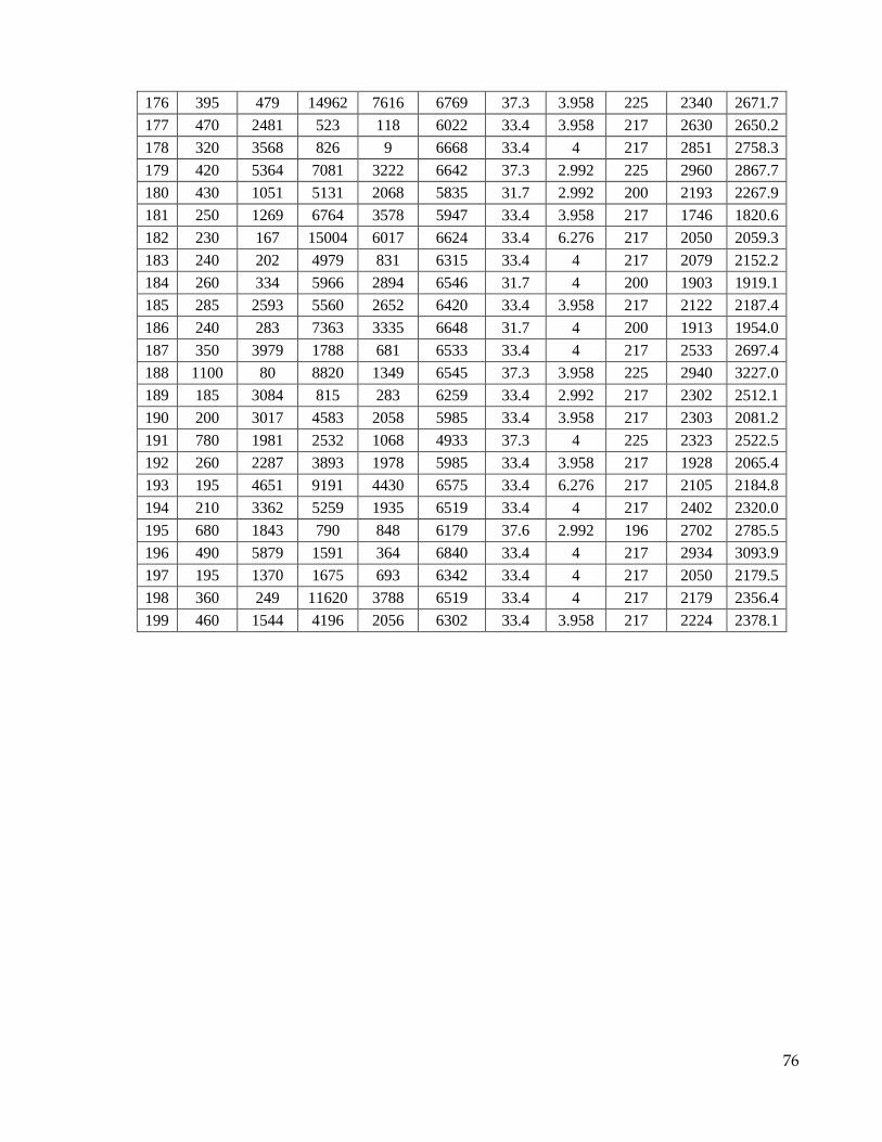
76
176 395 479 14962 7616 6769 37.3 3.958 225 2340 2671.7
177 470 2481 523 118 6022 33.4 3.958 217 2630 2650.2
178 320 3568 826 9 6668 33.4 4 217 2851 2758.3
179 420 5364 7081 3222 6642 37.3 2.992 225 2960 2867.7
180 430 1051 5131 2068 5835 31.7 2.992 200 2193 2267.9
181 250 1269 6764 3578 5947 33.4 3.958 217 1746 1820.6
182 230 167 15004 6017 6624 33.4 6.276 217 2050 2059.3
183 240 202 4979 831 6315 33.4 4 217 2079 2152.2
184 260 334 5966 2894 6546 31.7 4 200 1903 1919.1
185 285 2593 5560 2652 6420 33.4 3.958 217 2122 2187.4
186 240 283 7363 3335 6648 31.7 4 200 1913 1954.0
187 350 3979 1788 681 6533 33.4 4 217 2533 2697.4
188 1100 80 8820 1349 6545 37.3 3.958 225 2940 3227.0
189 185 3084 815 283 6259 33.4 2.992 217 2302 2512.1
190 200 3017 4583 2058 5985 33.4 3.958 217 2303 2081.2
191 780 1981 2532 1068 4933 37.3 4 225 2323 2522.5
192 260 2287 3893 1978 5985 33.4 3.958 217 1928 2065.4
193 195 4651 9191 4430 6575 33.4 6.276 217 2105 2184.8
194 210 3362 5259 1935 6519 33.4 4 217 2402 2320.0
195 680 1843 790 848 6179 37.6 2.992 196 2702 2785.5
196 490 5879 1591 364 6840 33.4 4 217 2934 3093.9
197 195 1370 1675 693 6342 33.4 4 217 2050 2179.5
198 360 249 11620 3788 6519 33.4 4 217 2179 2356.4
199 460 1544 4196 2056 6302 33.4 3.958 217 2224 2378.1

77
APPENDIX C
PROGRAM LISTING

78
C.1: Program for Calculating BHP in Prosper
Dim i As Integer Dim j As Integer Dim k As Integer = 10 Dim arr(6) As Integer arr(0) = 0 arr(1) = 1 arr(2) = 2 arr(3) = 4 arr(4) = 5 arr(5) = 9 arr(6) = 10 Dim aa As Integer xlApp = New Microsoft.Office.Interop.Excel.Application xlApp.Visible = True xlWorkBook = xlApp.Workbooks.Open("C:\Users\shamat0e\Desktop\AI\Project\data_for_Trend_Anls_Prosper.xls") Pxserver.connect() Pxserver.DoCommand("PROSPER.START") Pxserver.DoCommand("PROSPER.OPENFILE(""C:\Users\shamat0e\Desktop\AI\Project\Prosper_Sample.out"")") For i = 1 To 5 xlWorkSheet = xlWorkBook.Sheets(i) For aa = 0 To 6 For j = 2 To 10 Pxserver.setValue("PROSPER.ANL.GRD.Tubing", arr(aa)) Pxserver.setValue("PROSPER.ANL.GRD.Pres", xlWorkSheet.Cells(j, 1).value) Pxserver.setValue("PROSPER.ANL.GRD.WC", xlWorkSheet.Cells(j, 2).value) Pxserver.setValue("PROSPER.ANL.GRD.Rate", xlWorkSheet.Cells(j, 3).value) Pxserver.setValue("PROSPER.ANL.GRD.GOR", Val(xlWorkSheet.Cells(j, 4).value)) Pxserver.setValue("PROSPER.PVT.Input.Solgor", Val(xlWorkSheet.Cells(j, 4).value)) Pxserver.setValue("PROSPER.SIN.EQP.Down.Data[1].Depth", xlWorkSheet.Cells(j, 5).value) Pxserver.setValue("PROSPER.SIN.EQP.Devn.Data[1].Md", xlWorkSheet.Cells(j, 5).value) Pxserver.setValue("PROSPER.SIN.EQP.Devn.Data[1].Tvd", xlWorkSheet.Cells(j, 5).value) Pxserver.setValue("PROSPER.SIN.EQP.Geo.Data[1].Md", xlWorkSheet.Cells(j, 5).value) Pxserver.setValue("PROSPER.SIN.EQP.Down.Data[1].TID", xlWorkSheet.Cells(j, 7).value) Pxserver.DoCommand("PROSPER.ANL.GRD.CALC") Dim Grad_Count Grad_Count = Pxserver.getValue("PROSPER.OUT.GRD.RESULTS[i][j][k].NUM") - 1 xlWorkSheet.Cells(j, k) = Pxserver.getValue("PROSPER.OUT.GRD.Results[0][0][0].Pres[" & Grad_Count & "]") Next j k += 1 Next aa k = 10 Next i

79
C.2: Main Matlab Program for Generating the ANFIS model
clc
clear all close all [data, text]= xlsread('data_for_FL.xls'); IP_data = data(:,1:8); TRG_data = data(:,9); trn_in = IP_data(1:596,:); trn_out = TRG_data(1:596,:); tst_in = IP_data(597:795,:); tst_out = TRG_data(597:795,:); fismat2 = genfis2(trn_in,trn_out,0.6); out_fis2 = anfis([trn_in trn_out],fismat2); genfis2_Pred_trn_out = evalfis(trn_in,out_fis2); genfis2_Pred_tst_out = evalfis(tst_in,out_fis2); fismat2 = setfis(fismat2, 'input', 1, 'name','WHP') fismat2 = setfis(fismat2, 'input', 2, 'name','Qw') fismat2 = setfis(fismat2, 'input', 3, 'name','Qo') fismat2 = setfis(fismat2, 'input', 4, 'name','Qg') fismat2 = setfis(fismat2, 'input', 5, 'name','Dpth') fismat2 = setfis(fismat2, 'input', 6, 'name','api') fismat2 = setfis(fismat2, 'input', 7, 'name','ID') fismat2 = setfis(fismat2, 'input', 8, 'name','Tres') fismat2 = setfis(fismat2, 'output', 1, 'name','BHP') [C,S] = subclust(trn_in, 0.6) getfis(fismat2) showrule(fismat2) plotfis(fismat2) ruleview(fismat2) success = xlswrite ('results fuzzy.xls',trn_out,'WC_GOR_QL_1', 'A2'); success = xlswrite ('results fuzzy.xls',genfis2_Pred_trn_out,'WC_GOR_QL_1', 'B2'); success = xlswrite ('results fuzzy.xls',tst_out,'WC_GOR_QL_1', 'f2'); success = xlswrite ('results fuzzy.xls',genfis2_Pred_tst_out,'WC_GOR_QL_1', 'g2');

80
C.3: Matlab Program for the ANFIS Trend Analysis
clc clear all close all [data, text]= xlsread('data_for_FL.xls'); [trend_data, text]= xlsread('data_for_Trend_Anls.xls'); IP_data = data(:,1:8); TRG_data = data(:,9); trn_in = IP_data(1:596,:); trn_out = TRG_data(1:596,:); fismat2 = genfis2(trn_in,trn_out,0.6); out_fis2 = anfis([trn_in trn_out],fismat2); genfis2_Pred_Trend_out = evalfis(trend_data,out_fis2); success = xlswrite ('data_for_Trend_Anls.xls',genfis2_Pred_Trend_out,'gas rate', 'J2');
C.4: Matlab Program for the Generating the Histograms
clc [data, text]= xlsread('data for histogram.xls'); Duns_Ros = data(:,1); Hagedorn_Brown = data(:,2); Fancher_Brown = data(:,3); Mukhairji_Brill = data(:,4); Beggs_Brill = data(:,5); Orkisweski = data(:,6); PETEX_II = data(:,7); ANFIS_Testing = data(:,8); ANFIS_Training = data(:,9); figure histfit(Duns_Ros) h = findobj(gca,'Type','patch'); set(h,'FaceColor','w','EdgeColor','k') title('Duns and Ros'); xlabel('Relative Error %'); ylabel('Frequency') set(gcf, 'color', 'White')

81
CURRICULUM VITAE
Name: Ahmad Tariq Al-Shammari
Nationality: Syrian
E-mail: [email protected]
Address: Post Office Box # 2148
Dhahran 31311
Eastern Province, Saudi Arabia
Education: Bachelor of Science in Mechanical Engineering, 2002
King Fahd University of Petroleum & Minerals,
Dhahran 31261, Saudi Arabia.
Master of Science in Petroleum Engineering, 2011
King Fahd University of Petroleum & Minerals
Dhahran 31261, Saudi Arabia.
Areas of
Interest: Well Performance, Production Optimization
Professional
Affiliations: Society of Petroleum Engineers (SPE)
Experience: Ahmad Al-Shammari joined the Petroleum Engineering Application
Services Department of Saudi Aramco in October 2002. He is a specialist in
several well performance and pipeline simulation packages that are heavily
used by various organizations in the company to perform studies related to
well production and injection optimization and multiphase flow systems in
pipeline networks. He conducted several software training sessions for
Saudi Aramco engineers and developed many computer applications that
automate the process of building and calibrating well performance models
using the corporate database