deep flows on the slope inshore of the kuril-kamchatka trench

Journal of Oceanography, Vol. 55, pp. 559 to 573. 1999

559Copyright The Oceanographic Society of Japan.

Keywords:⋅Deep flow on slope,⋅Oyashio,⋅Kuril-KamchatkaTrench,

⋅ current measure-ment.

Deep Flows on the Slope Inshore of the Kuril-KamchatkaTrench Southeast off Cape Erimo, Hokkaido

KAZUYUKI UEHARA* and HIDEO MIYAKE

Laboratory of Physical Oceanography, Department of Fisheries Oceanography and Marine Science,Faculty of Fisheries, Hokkaido University, Minato-cho 3-1-1, Hakodate, Hokkaido 041-8611, Japan

(Received 28 March 1997; in revised form 4 February 1999; accepted 13 March 1999)

Deep flows on the slope inshore of the Kuril-Kamchatka Trench southeast off CapeErimo, Hokkaido were observed for about five years from June 1989 to March 1995, usinga mooring system with two current meters. In 1991 and 1993 directionally stablesouthwestward flows were observed at the upper layer (1000 m). These appear to betypical of the Oyashio because the characteristics of the flows were high mean kineticenergy, low eddy energy and high stability. However, the magnitudes of other mean flowsat the upper layer, except for 1991 and 1993, were less than their standard deviations. Thissuggests that the Oyashio was observed for only a limited period of time. On the otherhand, at the lower layer (3000 m) the magnitudes of the mean flows for 10–11 months were1–3 cm s–1 and ellipses of their eddy kinetic energy were extremely flattened in thedirection of the local isobath. The directions of the mean flows in 1990, 1991 and 1993 weresouthwestward along the local isobath. The relationships between the upper and the lowerflows are discussed in terms of monthly change of kinetic energy, since the low-frequencyfluctuations longer than 30-day are predominant from the eddy kinetic energy spectra.The results show that there are cases when the kinetic energy of the monthly mean flowsat the lower layers are larger than those at the upper layers. This suggests the possibilitythat the lower flows are in part a southward deep western boundary current.

in the North Pacific, considering the water properties in theearlier investigations. Moreover, they proposed a deep cir-culation scenario in the Northwest Pacific Basin based ontheir mooring observations coupled with the earlier obser-vational studies.

We have measured deep flows at 3000 m depth on theslope southeast off Cape Erimo, inshore of the southern endof the Kuril-Kamchatka Trench, to investigate the charac-teristics of deep flows near the western boundary region inthe Northwest Pacific Basin. The Oyashio, which is awestern boundary current of a surface circulation in thesubarctic gyre, also flows southwestward in this region.Therefore, the deep flows on the slope are considered tointeract with the Oyashio. Uehara et al. (1997) observed theOyashio southeast off Cape Erimo using mooring systems.They reported that the characteristics of the Oyashio arehigh kinetic energy of the mean flow, low eddy energy andhigh stability. In addition, the most intense and directionallystable flows usually occur in February. The purpose of thisstudy is to discuss the relationships between the deep flowson the slope inshore of the Kuril-Kamchatka Trench and theOyashio.

In this paper we first report some results of our currentmeasurements on the slope and reveal the statistical prop-

1. IntroductionObservations of the deep flows have been made since

Stommel and Arons (1960a, b) presented the abyssal cir-culation theory. However, characteristics of deep flows nearthe boundary region in the North Pacific are not known indetail owing to an insufficient number of deep currentmeasurements. Warren and Owens (1985, 1988) observeddeep flows across the Aleutian Trench in the central NorthPacific, using mooring systems and deep hydrographicsurveys. They obtained mean westward flow values of 1–3cm s–1 over fourteen months at 2000–3000 m depths alongthe slope inshore of the Aleutian Trench, and explainedthese as a northern boundary current, as required by theStommel and Arons model (1960a). Recently, Hallock andTeague (1996) obtained over two years mean southwardflows of 0.5–2.6 cm s–1 between 2000 m and the bottom near36°N, inshore of the Japan Trench. They concluded thatthese southward flows are a deep western boundary current

*Now at Physical Oceanography Section, Mixed WaterRegion Fisheries Oceanography Division, Tohoku National Fish-eries Research Institute, Shinhama-cho 3-27-5, Shiogama, Miyagi985-0001, Japan.

560 K. Uehara and H. Miyake

erties of the measured flows. Second, we investigate therelationship between the Oyashio and deep flows on theslope. Finally, we discuss the deep flows on the slope.

2. Mooring System and DataThe locations of the mooring station along the 41°30′

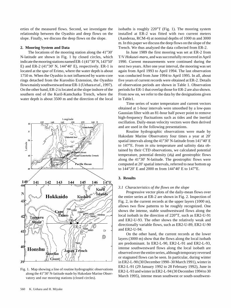
N-latitude are shown in Fig. 1 by closed circles, whichindicate the mooring stations named ER-1 (41°30′ N, 143°50′E) and ER-2 (41°30′ N, 144°40′ E), respectively. ER-1 islocated at the spur of Erimo, where the water depth is about1750 m. When the Oyashio is not influenced by warm-corerings detached from the Kuroshio Extension, the Oyashioflows mainly southwestward near ER-1 (Uehara et al., 1997).On the other hand, ER-2 is located at the slope inshore of thesouthern end of the Kuril-Kamchatka Trench, where thewater depth is about 3500 m and the direction of the local

Fig. 1. Map showing a line of routine hydrographic observationsalong the 41°30′ N-latitude made by Hakodate Marine Obser-vatory and our mooring stations (closed circles).

isobaths is roughly 220°T (Fig. 1). The mooring systeminstalled at ER-2 was fitted with two current meters(Aanderaa, RCM-4) at nominal depths of 1000 m and 3000m. In this paper we discuss the deep flows on the slope of theTrench. We thus analyzed the data collected from ER-2.

In June 1989 the first mooring was set at ER-2 fromT/V Hokusei-maru, and was successfully recovered in April1990. Current measurements were continued during thenext two years. After one year interval, the mooring was setagain from April 1993 to April 1994. The last observationwas conducted from June 1994 to April 1995. In all, aboutfive years of current records were obtained at ER-2. Detailsof observation periods are shown in Table 1. Observationperiods for ER-1 that overlap those for ER-2 are also shown.From now on, we refer to the data by the designations givenin Table1.

Time series of water temperature and current vectorsobtained at 1-hour intervals were smoothed by a low-passGaussian filter with an 81-hour half power point to removehigh-frequency fluctuations such as tides and the inertialoscillation. Daily-mean velocity vectors were then derivedand are used in the following presentations.

Routine hydrographic observations were made byHakodate Marine Observatory four times a year at 20′spatial intervals along the 41°30′ N-latitude from 141°40′ Eto 147°E. From in situ temperature and salinity data ob-tained by their CTD observations, we calculated potentialtemperature, potential density (σθ) and geostrophic flowsalong the 41°30′ N-latitude. The geostrophic flows werecomputed at 20′ spatial intervals, referred to near bottom upto 144°20′ E and 2000 m from 144°40′ E to 147°E.

3. Results

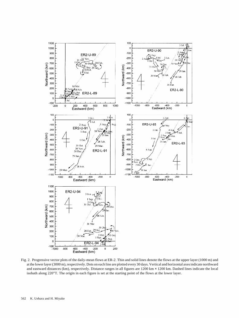
3.1 Characteristics of the flows on the slopeProgressive vector plots of the daily-mean flows over

the entire series at ER-2 are shown in Fig. 2. Inspection ofFig. 2, in the current records at the upper layers (1000 m),allows two flow patterns to be roughly recognized. Oneshows the intense, stable southwestward flows along thelocal isobath in the direction of 220°T, such as ER2-U-91and ER2-U-93. The other shows the relatively weak anddirectionally variable flows, such as ER2-U-89, ER2-U-90and ER2-U-94.

On the other hand, the current records at the lowerlayers (3000 m) show that the flows along the local isobathare predominant. In ER2-L-90, ER2-L-91 and ER2-L-93,intense southwestward flows along the local isobath areobserved over the entire series, although temporary reversedor stagnated flows can be seen. In particular, during winterin ER2-L-90 (30 December 1990–30 March 1991), winter inER2-L-91 (29 January 1992 to 28 February 1992), June inER2-L-93 and winter in ER2-L-94 (30 December 1994 to 30March 1995), intense mean southwest or south-southwest-

Deep Flows on the Slope Inshore of the Kuril-Kamchatka Trench Southeast off Cape Erimo 561

Table 1. The periods and instrument depths of current measurements off Cape Erimo.

ER-1: 41°30′ N, 143°30′ E; ER-1*: 41°30′ N, 144°00′ E; ER-2: 41°30′ N, 144°30′ E.

ward flows exceeding about 6 cm s–1 are observed. Fur-thermore, northeastward flows along the local isobath areobserved in ER2-L-89 and the first half of ER2-L-94,although they are weak.

We calculated statistics of these flows to investigatethe characteristics of the flows on the slope. We first com-puted the currents in a rotated system of along-isobath(+u = 220°T southwest, alongslope) and cross-isobath (+v =130°T downslope), because the flows at lower layer arepredominant along the local isobath (Fig. 2). The alongslopecomponents of the daily-mean flow u and the downslopecomponents v are represented as follows,

u = u + u′ , v = v + v′ , 1( )

where the

u ,

v indicate the mean values of u, v, averagedover the entire series. The primed symbols u′ , v′ indicatefluctuating components of the u, v, respectively.

We then computed the kinetic energy of the mean flowaveraged over the entire series per unit mass from Eq. (1),

KE = 12

u 2 + v 2( ). 2( )

In the same way, the eddy kinetic energy per unit mass wascomputed as follows,

KE ′ = 12

u′ 2 + v′ 2( ) = 12

σu2 + σv

2( ), 3( )

where σu2, σv

2 are the variance of the u, v, respectively.

The standard error of the mean of the u and v (εu and εv)was computed by first determining the integral timescale τ i

for each u, v time series by integrating the normalized auto-correlation functions. For estimating the integral timescale,we used the computed correlation functions, summed out tothe first zero crossing. The error then is ε = (2σ2τ i/T)1/2, whereT is a record length. These statistics are listed in Table 2.3.1.1 The mean flow field at the upper layer (1000 m)

In ER2-U-91 and ER2-U-93 the magnitudes of themean velocity vectors exceeded 4 cm s–1 and were greaterthan their standard deviations (Table 2). Their directionswere 203°T and 211°T, southwestward and approximatelyalong the local isobath. In particular, the flow characteristicsin ER2-U-91 are high

KE and low KE′ , therefore, the ratioof eddy to mean kinetic energy, KE′/

KE , is less than 1.Although the KE′/

KE ratio in ER2-U-93 is slightly greaterthan 1,

KE in ER2-U-93 is the same magnitude as in ER2-U-91. These flows show that the mean flow along the localisobath is more predominant than the fluctuating component.These flow characteristics are almost the same of that inER1-U-91 and ER1-U-93 which are located in the core ofthe Oyashio (Uehara et al., 1997). In others at the upperlayers, however, the magnitudes of the mean velocities wereless than their standard deviations. In particular, the stan-dard errors, εv, in ER2-U-89 and ER2-U-90 are larger thantheir mean values. These flows are characterized by low

KE , high KE′, therefore, the KE′/

KE ratios are very muchlarger than 1. That is, the fluctuating components are morepredominant than the mean flows in these flows. What is thedifference in the flow characteristics between the formerand the latter?

Vertical sections of CTD observations and the geostro-

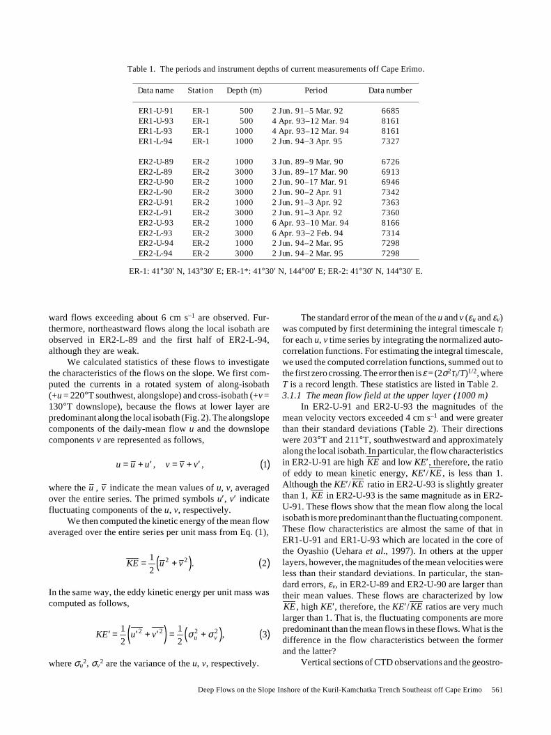
Data name Station Depth (m) Period Data number

ER1-U-91 ER-1 500 2 Jun. 91–5 Mar. 92 6685ER1-U-93 ER-1 500 4 Apr. 93–12 Mar. 94 8161ER1-L-93 ER-1 1000 4 Apr. 93–12 Mar. 94 8161ER1-L-94 ER-1 1000 2 Jun. 94–3 Apr. 95 7327

ER2-U-89 ER-2 1000 3 Jun. 89–9 Mar. 90 6726ER2-L-89 ER-2 3000 3 Jun. 89–17 Mar. 90 6913ER2-U-90 ER-2 1000 2 Jun. 90–17 Mar. 91 6946ER2-L-90 ER-2 3000 2 Jun. 90–2 Apr. 91 7342ER2-U-91 ER-2 1000 2 Jun. 91–3 Apr. 92 7363ER2-L-91 ER-2 3000 2 Jun. 91–3 Apr. 92 7360ER2-U-93 ER-2 1000 6 Apr. 93–10 Mar. 94 8166ER2-L-93 ER-2 3000 6 Apr. 93–2 Feb. 94 7314ER2-U-94 ER-2 1000 2 Jun. 94–2 Mar. 95 7298ER2-L-94 ER-2 3000 2 Jun. 94–2 Mar. 95 7298


Fig. 2. Progressive vector plots of the daily-mean flows at ER-2. Thin and solid lines denote the flows at the upper layer (1000 m) andat the lower layer (3000 m), respectively. Dots on each line are plotted every 30 days. Vertical and horizontal axes indicate northwardand eastward distances (km), respectively. Distance ranges in all figures are 1200 km × 1200 km. Dashed lines indicate the localisobath along 220°T. The origin in each figure is set at the starting point of the flows at the lower layer.


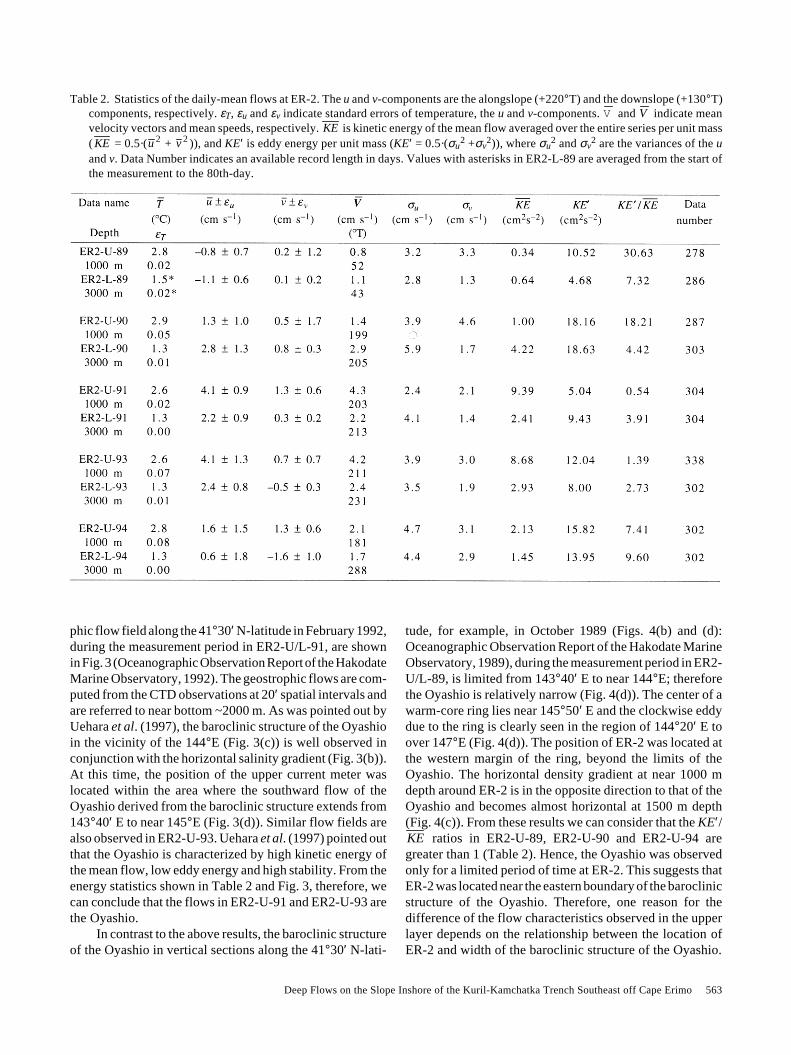
Table 2. Statistics of the daily-mean flows at ER-2. The u and v-components are the alongslope (+220°T) and the downslope (+130°T)components, respectively. εT, εu and εv indicate standard errors of temperature, the u and v-components.

V and

V indicate meanvelocity vectors and mean speeds, respectively.

KE is kinetic energy of the mean flow averaged over the entire series per unit mass(

KE = 0.5·(

u 2 +

v 2 )), and KE′ is eddy energy per unit mass (KE′ = 0.5·(σu2 +σv

2)), where σu2 and σv

2 are the variances of the uand v. Data Number indicates an available record length in days. Values with asterisks in ER2-L-89 are averaged from the start ofthe measurement to the 80th-day.

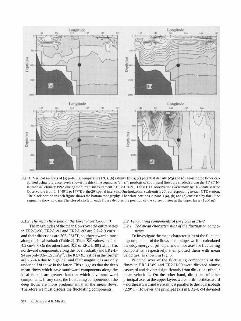
phic flow field along the 41°30′ N-latitude in February 1992,during the measurement period in ER2-U/L-91, are shownin Fig. 3 (Oceanographic Observation Report of the HakodateMarine Observatory, 1992). The geostrophic flows are com-puted from the CTD observations at 20′ spatial intervals andare referred to near bottom ~2000 m. As was pointed out byUehara et al. (1997), the baroclinic structure of the Oyashioin the vicinity of the 144°E (Fig. 3(c)) is well observed inconjunction with the horizontal salinity gradient (Fig. 3(b)).At this time, the position of the upper current meter waslocated within the area where the southward flow of theOyashio derived from the baroclinic structure extends from143°40′ E to near 145°E (Fig. 3(d)). Similar flow fields arealso observed in ER2-U-93. Uehara et al. (1997) pointed outthat the Oyashio is characterized by high kinetic energy ofthe mean flow, low eddy energy and high stability. From theenergy statistics shown in Table 2 and Fig. 3, therefore, wecan conclude that the flows in ER2-U-91 and ER2-U-93 arethe Oyashio.

In contrast to the above results, the baroclinic structureof the Oyashio in vertical sections along the 41°30′ N-lati-

tude, for example, in October 1989 (Figs. 4(b) and (d):Oceanographic Observation Report of the Hakodate MarineObservatory, 1989), during the measurement period in ER2-U/L-89, is limited from 143°40′ E to near 144°E; thereforethe Oyashio is relatively narrow (Fig. 4(d)). The center of awarm-core ring lies near 145°50′ E and the clockwise eddydue to the ring is clearly seen in the region of 144°20′ E toover 147°E (Fig. 4(d)). The position of ER-2 was located atthe western margin of the ring, beyond the limits of theOyashio. The horizontal density gradient at near 1000 mdepth around ER-2 is in the opposite direction to that of theOyashio and becomes almost horizontal at 1500 m depth(Fig. 4(c)). From these results we can consider that the KE′/

KE ratios in ER2-U-89, ER2-U-90 and ER2-U-94 aregreater than 1 (Table 2). Hence, the Oyashio was observedonly for a limited period of time at ER-2. This suggests thatER-2 was located near the eastern boundary of the baroclinicstructure of the Oyashio. Therefore, one reason for thedifference of the flow characteristics observed in the upperlayer depends on the relationship between the location ofER-2 and width of the baroclinic structure of the Oyashio.


Fig. 3. Vertical sections of (a) potential temperature (°C), (b) salinity (psu), (c) potential density (σθ) and (d) geostrophic flows cal-culated using reference levels shown the thick line segments (cm s–1; portions of southward flows are shaded) along the 41°30′ N-latitude in February 1992, during the current measurement in ER2-U/L-91. These CTD observations were made by Hakodate MarineObservatory from 141°40′ E to 147°E at the 20′ spatial intervals. One horizontal scale unit is 20′, corresponding to each CTD station.The black portion in each figure shows the bottom topography. The white portions in panels (a), (b) and (c) enclosed by thick linesegments show no data. The closed circle in each figure denotes the position of the current meter at the upper layer (1000 m).

3.1.2 The mean flow field at the lower layer (3000 m)The magnitudes of the mean flows over the entire series

in ER2-L-90, ER2-L-91 and ER2-L-93 are 2.2–2.9 cm s–1

and their directions are 205–231°T, southwestward almostalong the local isobath (Table 2). Their

KE values are 2.4–4.2 cm2s–2. On the other hand,

KE of ER2-L-89 (which hasnorthward components along the local isobath) and ER2-L-94 are only 0.6–1.5 cm2s–2. The KE′/

KE ratios in the formerare 2.7–4.4 due to high

KE and their magnitudes are onlyunder half of those in the latter. This suggests that the deepmean flows which have southward components along thelocal isobath are greater than that which have northwardcomponents. In any case, the fluctuating components of thedeep flows are more predominant than the mean flows.Therefore we must discuss the fluctuating components.

3.2 Fluctuating components of the flows at ER-23.2.1 The mean characteristics of the fluctuating compo-

nentsTo investigate the mean characteristics of the fluctuat-

ing components of the flows on the slope, we first calculatedthe eddy energy of principal and minor axes for fluctuatingcomponents, respectively, then plotted them with meanvelocities, as shown in Fig. 5.

Principal axes of the fluctuating components of theflows in ER2-U-89 and ER2-U-90 were directed almosteastward and deviated significantly from directions of theirmean velocities. On the other hand, directions of otherprincipal axes at the upper layers were north-northeastward~ northeastward and were almost parallel to the local isobath(220°T). However, the principal axis in ER2-U-94 deviated


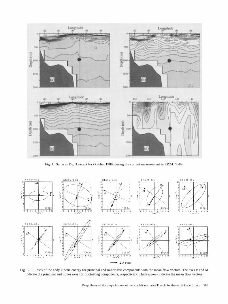
Fig. 4. Same as Fig. 3 except for October 1989, during the current measurement in ER2-U/L-89.

Fig. 5. Ellipses of the eddy kinetic energy for principal and minor axis components with the mean flow vectors. The axes P and Mindicate the principal and minor axes for fluctuating components, respectively. Thick arrows indicate the mean flow vectors.

566K

. Uehara and H

. Miyake

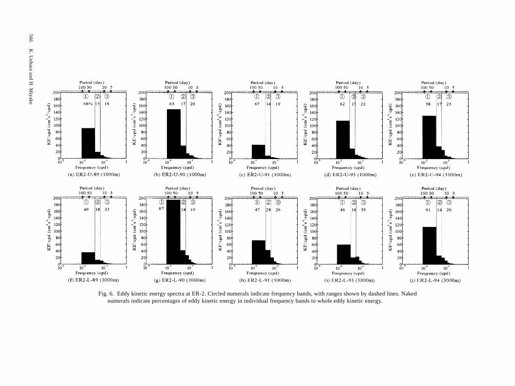
Fig. 6. Eddy kinetic energy spectra at ER-2. Circled numerals indicate frequency bands, with ranges shown by dashed lines. Nakednumerals indicate percentages of eddy kinetic energy in individual frequency bands to whole eddy kinetic energy.


from its mean velocity. In contrast to this, the principal axesin ER2-U-91 and ER2-U-93, which were observed theOyashio, agreed with directions of their mean velocities.Moreover, the ellipses of the eddy energy at ER2-U-91 arenearly circular, and flow variability shows isotropy.

In the lower layers, the directions of the principal axesof the fluctuating components agreed with those of the meanvelocities and were parallel to the local isobath (220°T),except for ER2-L-94. Moreover, ellipses of eddy kineticenergy were extremely flattened in the direction of the localisobath. This shows that the deep flows here were controlledby the local bottom topography. The magnitudes of the eddykinetic energy of the principal axes at the lower layers werecomparable to, or larger than those at the upper layers.3.2.2 Spectra of the eddy kinetic energy

We computed frequency spectra of the eddy kineticenergy, to investigate predominant periods of the flowfluctuations on the slope. To compute the eddy kineticenergy spectra, we first computed the spectra from timeseries of u′ and v′ , using the direct Fourier transform method.Next, these spectra were smoothed by averaging over fourfrequencies to obtain consistency of spectral estimates. Wethen obtained the total eddy kinetic energy spectra as thesum of spectra for u′ and v′ . These spectra are shown in Fig.6. For convenience, each spectrum is divided into threefrequency bands. Band (1) is the lowest frequency band,ranging from about 120- to 30-day periods. Band (2) is theintermediate frequency band, ranging from 30- to 16-dayperiods. Band (3) is the highest frequency band, less than 16-day.

In the upper layers, spectral distributions are charac-terized by a rapid decrease in energy toward higher frequen-cies. That is, the energy level in band (1) is the highest ineach frequency band. The contributions of the eddy kineticenergy in the lowest frequency band (1) to the whole eddykinetic energy in all frequencies are more than about 60%.Moreover, the contributions in frequency bands (1) and (2)to the whole eddy kinetic energy are more than 75%. Thus,the flow fluctuations at the upper layers shown in Fig. 5 aredue to the low-frequency fluctuations.

In the lower layers, the eddy kinetic energy levels in thelowest frequency band (1) in ER2-L-89, 93 and 94 are notvery large in comparison with those in the upper layers. Bycontrast, those in ER2-L-90 and 91 are larger than those inER2-U-90 and 91. In addition, in higher-frequency regions,bands (2) and (3), the eddy kinetic energy levels at the lowerlayers are generally larger than those at the upper layers.However, the contributions in these higher-frequency bandsto the whole eddy kinetic energy are small. The highestcontribution to the whole eddy kinetic energy is from theeddy kinetic energy in the lowest frequency band (1), thesame as in the upper layers. Therefore, low-frequency fluc-tuations of the flows are more predominant at the lowerlayers, in the same way as those at the upper layers.

3.3 Relationships between the upper flows and the lowerflowsNext we examine the relationships between the upper

and the lower flows from the monthly kinetic energy levels,because considerable variations in the flows over timescales of months or so are indicated by the eddy kineticenergy spectra (Fig. 6). Here we calculated the kineticenergy of the monthly mean flows, ⟨KE⟩ , as follows,

KE = 12

u 2 + v 2( ), 4( )

where the brackets ⟨ ⟩ indicate monthly mean, that is, ⟨u⟩ , ⟨v⟩are the monthly mean flows of the alongslope (220°T),downslope components (130°T), respectively. In addition,the monthly eddy kinetic energy to the monthly mean flows,KE*, are calculated as

KE∗ = 12

u∗ 2 + v∗ 2( ), 5( )

where ⟨u*2⟩ , ⟨v*2⟩ are the variance of the monthly flows.Hence, the monthly mean of the kinetic energy,

KEm , be-comes

KEm = 12

u 2 + v 2( )= KE + KE∗ . 6( )

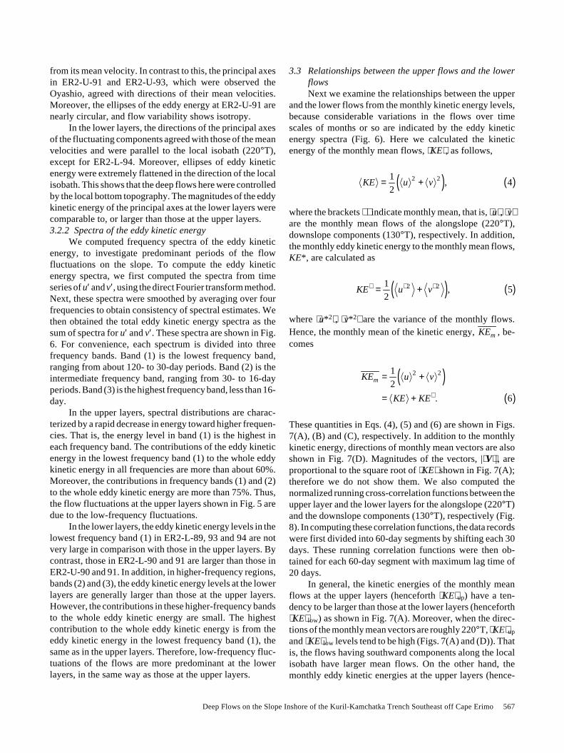
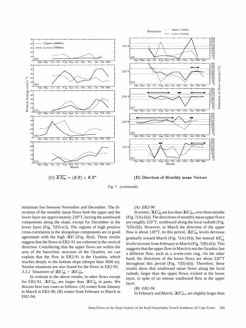
These quantities in Eqs. (4), (5) and (6) are shown in Figs.7(A), (B) and (C), respectively. In addition to the monthlykinetic energy, directions of monthly mean vectors are alsoshown in Fig. 7(D). Magnitudes of the vectors, |⟨V⟩ |, areproportional to the square root of ⟨KE⟩ shown in Fig. 7(A);therefore we do not show them. We also computed thenormalized running cross-correlation functions between theupper layer and the lower layers for the alongslope (220°T)and the downslope components (130°T), respectively (Fig.8). In computing these correlation functions, the data recordswere first divided into 60-day segments by shifting each 30days. These running correlation functions were then ob-tained for each 60-day segment with maximum lag time of20 days.

In general, the kinetic energies of the monthly meanflows at the upper layers (henceforth ⟨KE⟩up) have a ten-dency to be larger than those at the lower layers (henceforth⟨KE⟩ low) as shown in Fig. 7(A). Moreover, when the direc-tions of the monthly mean vectors are roughly 220°T, ⟨KE⟩up

and ⟨KE⟩ low levels tend to be high (Figs. 7(A) and (D)). Thatis, the flows having southward components along the localisobath have larger mean flows. On the other hand, themonthly eddy kinetic energies at the upper layers (hence-


forth

KEup∗ ) have a tendency to be less than those at the lower

layers (henceforth

KElow∗ ) as shown in Fig. 7(B). This sug-

gests that higher-frequency fluctuations (under a month) atthe lower layers are more predominant than those at theupper layers. The values of the cross-correlations in thedirection of 220°T between the upper and the lower layersare higher than those in the direction of 130°T (Fig. 8). Inaddition to this, the high positive cross-correlations are ingood agreement with both higher ⟨KE⟩ (Fig. 7(A)) and theflows in the direction of 220°T (Fig. 7(D)). In particular,each ⟨KE⟩ series has a peak in winter, and cross-correlationvalues more than 0.6 are found in winter after January,except for ER2-89, although, unfortunately, there is nocross-correlation data for winter in ER2-93 (Fig. 8(g)).

From these results, we consider that the flows along the localisobath which have higher ⟨KE⟩ are vertically coherent.

To describe relationships of the flows between theupper and the lower layers, we discuss some concreteexamples. Firstly, we examine situations of ⟨KE⟩up > ⟨KE⟩ low,such as ER2-91 (Fig. 7(A)-(c)). Contrary to this, secondly,we also examine some situations of ⟨KE⟩up < ⟨KE⟩ low. Fi-nally, we mention the northeastward flows along the localisobath, such as ER2-89 (Figs. 7(A)-(a) and 7(D)-(a)).3.3.1 Situations of ⟨KE⟩up > ⟨KE⟩ low

During period in ER2-91, ⟨KE⟩up are larger than ⟨KE⟩ low

for all months (Fig. 7(A)-(c)). Variations by months in⟨KE⟩up and ⟨KE⟩ low are almost the same; there is the maxi-mum peak in February, September follows this, and the

Fig. 7. (A) The kinetic energy of the monthly mean flows ⟨KE⟩ , (a) ER2-89, (b) ER2-90, (c) ER2-91, (d) ER2-93 and (e) ER2-94. Thinand thick lines indicate the upper layers ⟨KE⟩up and the lower layers ⟨KE⟩ low, respectively. Arrows indicate the periods when⟨KE⟩ low > ⟨KE⟩up. (B) The monthly eddy kinetic energy KE*, (a) ER2-89, (b) ER2-90, (c) ER2-91, (d) ER2-93 and (e) ER2-94. Thin

and thick lines indicate the upper layers

KEup∗ and the lower layers

KElow∗ , respectively. (C) The monthly mean of the kinetic energy

KEm , (a) ER2-89, (b) ER2-90, (c) ER2-91, (d) ER2-93 and (e) ER2-94. Thin and thick lines indicate the upper layers and the lowerlayers, respectively. (D) The directions of the monthly mean flows. Three horizontal lines indicate 265°T, 220°T and 175°T at 45intervals, respectively. Arrows show the periods when monthly mean flow directions are southwestward, roughly 220°T in both theupper and the lower layers.


minimum lies between November and December. The di-rections of the monthly mean flows both the upper and thelower layer are approximately 220°T, having the southwardcomponents along the slope, except for December in thelower layer (Fig. 7(D)-(c)). The regions of high positivecross-correlation in the alongslope components are in goodagreement with the high ⟨KE⟩ (Fig. 8(e)). These resultssuggest that the flows in ER2-91 are coherent in the verticaldirection. Considering that the upper flows are within thearea of the baroclinic structure of the Oyashio, we canexplain that the flow in ER2-91 is the Oyashio, whichreaches deeply to the bottom slope (deeper than 3000 m).Similar situations are also found for the flows in ER2-93.3.3.2 Situations of ⟨KE⟩up > ⟨KE⟩ low

In contrast to the above results, in other flows exceptfor ER2-91, ⟨KE⟩ low are larger than ⟨KE⟩up in parts. Wediscuss here two cases as follows: (A) winter from Januaryto March in ER2-90, (B) winter from February to March inER2-94.

(A) ER2-90In winter, ⟨KE⟩up are less than ⟨KE⟩ low over three months

(Fig. 7(A)-(b)). The directions of monthly mean upper flowsare roughly 220°T, southward along the local isobath (Fig.7(D)-(b)). However, in March the direction of the upperflow is about 120°T. In this period, ⟨KE⟩up levels decrease

gradually toward March (Fig. 7(A)-(b)), but instead

KEup∗

levels increase from February to March (Fig. 7(B)-(b)). Thissuggests that the upper flow in March is not the Oyashio, buta different flow, such as a worm-core ring. On the otherhand, the directions of the lower flows are about 220°Tthroughout this period (Fig. 7(D)-(b)). Therefore, theseresults show that southward mean flows along the localisobath, larger than the upper flows, existed at the lowerlayer, in spite of no intense southward flow at the upperlayer.

(B) ER2-94In February and March, ⟨KE⟩ low are slightly larger than

Fig. 7. (continued).


⟨KE⟩up (Fig. 7(A)-(e)), and both of them are larger than

KElow∗ and

KEup∗ , respectively (Fig. 7(B)-(e)). The direc-

tions of the monthly mean flows at both the upper and thelower layer are roughly 220°T, having southward compo-nents along the local isobath (Fig. 7(D)-(e)). At this time thecross-correlations are high in the direction of 220°T (Fig.8(i)). These facts show that both the upper and the lowerflows are stable, intense southward flows during fromFebruary to March and are coherent. Similar situations arefound in June of ER2-93.

3.3.3 Northeastward flows along the local isobathIn ER2-89, the directions of the monthly mean flows at

the lower layers are about 30°T–60°T, having northwardcomponents, from July to November (Fig. 7(D)-(a)). ⟨KE⟩ low

are quite small in this period (Fig. 7(A)-(a)), therefore, thelower flows in ER2-89 are very weak and not stable. How-ever, the cross-correlations between the upper and the lowerflows are relatively high to December (Fig. 8(a)), in spite ofthe fact that the directions of the lower flows are not inagreement with those of the upper layer (Fig. 7(D)-(a)).

Fig. 8. The normalized cross-correlation functions between the upper flows and the lower flows. Left side panels are for the alongslopecomponents (220°T) and right side panels are for the downslope components (130°T). Contour intervals are 0.2. Shaded portionsindicate statistically significant correlation values (significant level of 95%). Arrows in the left panels show the period when cross-correlations are positive and more than 0.6.


4. Discussion

4.1 Schematic flow images on the slopeTo explain the flows on the slope at ER-2, we consid-

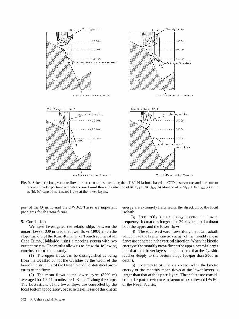
ered four schematic flow images as follows. When thebaroclinic structure of the Oyashio extends to the eastbeyond the position of ER-2, such as ER2-U-91 (see Fig. 3),the flows on the slope are intense, stable southward flowsalong the local isobath in both the upper and the lowerlayers. At this time, the flows on the slope are coherent in thevertical direction, and the upper flows are more intense thanthe lower flows. Therefore, we can explain that the Oyashioreaches deeply to the near bottom slope (deeper than 3000m). This flow image can be illustrated schematically in Fig.9(a). On the other hand, there are roughly two cases when⟨KE⟩up are less than ⟨KE⟩ low. If the Oyashio reaches deeplyto the lower layer, ⟨KE⟩up must be larger than ⟨KE⟩ low, suchas ER2-91. How can we give an explanation for these larger⟨KE⟩ low?

One case is the situation of ER2-94 in February andMarch. In this period, the upper flows are intense, stable,southwestward flows, the same as ER2-U-91 in winter.However, the lower flows, which are southward along thelocal isobath, are more intense than the upper flows. Fromhigh cross-correlations between the upper and the lowerflows, it is considered that these southwestward flows at thelower layer are lower parts of the Oyashio. However, theexplanation of ⟨KE⟩up < ⟨KE⟩ low cannot found from only inthe Oyashio. That is, we can consider that the situation of⟨KE⟩up < ⟨KE⟩ low are one item of evidence for a southwarddeep western boundary current in the North Pacific (DWBC)along the slope. The lower flows here, therefore, can beexplained in terms of an overlap between the lower part ofthe Oyashio and the DWBC, as illustrated in Fig. 9(b).

The other case is the situation of ER2-90 in winter fromJanuary to March. In January and February, the flow imageis similar to ER2-94 (Fig. 9(b)). We should draw the reader’sattention now to the flows in March. In March the directionof the upper flows is 120°T, not along the slope (Fig. 7(D)-

(b)), and ⟨KE⟩up is quite small, but

KEup∗ is now large.

Therefore, the upper flow in March is unstable and cannot bethe Oyashio. On the other hand, the lower flows are stableand intense along the slope, having a southwestward com-ponent. Hence, it is considered that this lower flow is alsoevidence of the DWBC (Fig. 9(c)).

When the lower flows are northward along the localisobath, such as ER2-89, the flow image is as shown in Fig.9(d). As shown in Fig. 4, the warm-core ring lies near ER-2 and the upper current meter is located in the northwardflow region of the ring. Therefore, it is supposed that thewarm-core ring influences the lower flows. But the north-ward flows are very weak and unstable.

In any case, we do not know at all how the DWBCdistributes on the slope around ER-2 in the inshore of the

Kuril-Kamchatka Trench, as marked “?” in Fig. 9(b), (c).Further study is necessary to clarify these problems.

4.2 Higher-frequency fluctuations under 30-day

In generally,

KElow∗ are larger than

KEup∗ (Fig. 7(B)).

This indicates that higher-frequency fluctuations under 30-day at the lower layer are predominant over those at theupper layers. This is also shown in the eddy kinetic energy

spectra (Fig. 6). Due to these large

KElow∗ , there are some

cases when the monthly mean of the kinetic energy

KEm atthe lower layers is larger than that at the upper layers, suchas August and September in ER2-90 (Fig. 7(C)-(b)),December and January in ER2-91 (Fig. 7(C)-(c)). Themooring system ER-2 is located on the steep slope in theKuril-Kamchatka Trench, and therefore, it is consideredthat the topographic β effect is not negligible for the higher-frequency fluctuations at the lower layers. Here, we roughlyestimate the value of the topographic β. Around ER-2, wemay assume that the slope gradient Γ ≈ 4.8 × 10–2, the waterdepth H ≈ 3500 (m) and the Coriolis parameter at the 41°30′N-latitude f ≈ 10–4 (s–1). Therefore, the value of the topo-graphic β becomes approximately 1.4 × 10–9 (m–1s–1), whichis two orders of magnitude larger than the planetary β at 41°30′N-latitude, which is approximately 1.7 × 10–11 (m–1s–1).Hence, we propose the possibility that the large eddy ener-gies at the lower layers are due to some topographic wavesdue to the topographic β effect. This seems to be a worth-while subject to investigate, and we want it to be the subjectof a future study.

4.3 Other deep flows on the slope inshore of the trenchesWarren and Owens (1985; henceforth WO) obtained

the 14-month mean deep flows of 1–3 cm s–1 at 2000–3000m depths along the slope inshore of the Aleutian Trench.Hallock and Teague (1996; henceforth HT) obtained the twoyears mean deep flows of 0.5–2.6 cm s–1 between 2000 mand near the bottom along the slope inshore of the JapanTrench. As results of our current measurements at 3000 mdepth (almost the same depths of WO and HT) on the slopeinshore of the Kuril-Kamchatka Trench, we obtained threedeep southwestward flows of 2.2–2.9 cm s–1 (ER2-L-90, ER2-L-91 and ER2-L-93) averaged for 10 or 11 months along theslope. The magnitudes and directions of these mean deepflows are similar to those of the flows observed by WO andHT. At this point, our three mean southwestward flows seemto be consistent with the deep circulation scenario proposedby HT, considering that our mooring location is inshore ofthe Kuril-Kamchatka Trench, where is located between theAleutian Trench (WO) and the Japan Trench (HT). How-ever, the observed northeastward flows such as ER2-L-89,contradict the HT scenario, but the cause for this is un-known. Furthermore, it is very difficult to distinguish thedeep flows on the slope obtained by us as between the lower


part of the Oyashio and the DWBC. These are importantproblems for the near future.

5. ConclusionWe have investigated the relationships between the

upper flows (1000 m) and the lower flows (3000 m) on theslope inshore of the Kuril-Kamchatka Trench southeast offCape Erimo, Hokkaido, using a mooring system with twocurrent meters. The results allow us to draw the followingconclusions from this study.

(1) The upper flows can be distinguished as beingfrom the Oyashio or not the Oyashio by the width of thebaroclinic structure of the Oyashio and the statistical prop-erties of the flows.

(2) The mean flows at the lower layers (3000 m)averaged for 10–11 months are 1–3 cm s–1 along the slope.The fluctuations of the lower flows are controlled by thelocal bottom topography, because the ellipses of the kinetic

energy are extremely flattened in the direction of the localisobath.

(3) From eddy kinetic energy spectra, the lower-frequency fluctuations longer than 30-day are predominantboth the upper and the lower flows.

(4) The southwestward flows along the local isobathwhich have the higher kinetic energy of the monthly meanflows are coherent in the vertical direction. When the kineticenergy of the monthly mean flow at the upper layers is largerthan that at the lower layers, it is considered that the Oyashioreaches deeply to the bottom slope (deeper than 3000 mdepth).

(5) Contrary to (4), there are cases when the kineticenergy of the monthly mean flows at the lower layers islarger than that at the upper layers. These facts are consid-ered to be partial evidence in favour of a southward DWBCof the North Pacific.

Fig. 9. Schematic images of the flows structure on the slope along the 41°30′ N-latitude based on CTD observations and our currentrecords. Shaded portions indicate the southward flows. (a) situation of ⟨KE⟩up > ⟨KE⟩ low, (b) situation of ⟨KE⟩up < ⟨KE⟩ low, (c) sameas (b), (d) case of northward flows at the lower layers.


6617–6624.Stommel, H. and A. B. Arons (1960a): On the abyssal circulation

of the world ocean—I. Stationary planetary flow patterns ona sphere. Deep-Sea Res., 6, 140–154.

Stommel, H. and A. B. Arons (1960b): On the abyssal circulationof the world ocean—II. An idealized model of the circulationpattern and amplitude in ocean basins. Deep-Sea Res., 6, 217–233.

Uehara, K., H. Miyake and M. Okazaki (1997): Characteristics ofthe flows in the Oyashio area off Cape Erimo, Hokkaido,Japan. J. Oceanogr., 53, 93–103.

Warren, B. A. and W. B. Owens (1985): Some preliminary resultsconcerning deep northern-boundary currents in the NorthPacific. Prog. Oceanogr., 14, 537–551.

Warren, B. A. and W. B. Owens (1988): Deep current in thecentral subarctic Pacific Ocean. J. Phys. Oceanogr., 18, 529–551.

AcknowledgementsWe would like to acknowledge the assistance, support,

and efforts of Dr. Kajihara as well as the others of thegraduate students of Laboratory of Physical Oceanography,Faculty of Fisheries, Hokkaido University. We wish tothank the officers and the crew of the T/S Hokusei-maru,Hokkaido University, who conducted the deployments andrecoveries of the current meter moorings. Comments fromtwo reviewers and Associate Editor, Dr. Jiro Yoshida, havegreatly improved the presentation of this paper.

ReferencesHakodate Marine Observatory (1989–1995): Oceanographic Ob-

servation Report, 27-33.Hallock, Z. R. and W. J. Teague (1996): Evidence for a North

Pacific deep western boundary current. J. Geophys. Res., 101,

deep flows on the slope inshore of the kuril-kamchatka trench

Documents