deep learning acceleration on the edge
TRANSCRIPT
Deep Learning Acceleration on the Edge
by Aditya Misra
A DISSERTATION
PRESENTED TO THE UNIVERSITY OF DUBLIN, TRINITY COLLEGE
IN PARTIAL FULFILMENT OF THE REQUIREMENTS FOR THE DEGREE OF
MASTER OF SCIENCE IN COMPUTER SCIENCE (INTELLIGENT SYSTEMS)
SUPERVISOR: PROFESSOR ROZENN DAHYOT
AUGUST 2019

©Aditya Misra August 15, 2019 Page 1/76
Declaration
I, the undersigned, declare that this thesis has not been submitted as an exercise for a degree at this or any
other university and and that unless otherwise stated, is my own work.
Aditya Misra
August 15, 2019

©Aditya Misra August 15, 2019 Page 2/76
Permission to Lend and/or Copy
I, the undersigned, agree that Trinity College Library may lend or copy this thesis upon request.
Aditya Misra
August 15, 2019
©Aditya Misra August 15, 2019 Page 3/76
Acknowledgments
I am extremely grateful to my parents without whom chasing this dream would have remained a fantasy.
To my supervisor, Prof. Dr. Rozenn Dahyot for her continuous support, guidance, encouragement and ex-
pertise during my Master thesis.
To Late Prof. Séamus Lawless, who provided me with the required hardware for this dissertation and will
continue to inspire me in the future through his example and dedication.
To the staff of Mama’s Revenge and Lavazza Coffee Machine for the regular supplies of Burritos and Coffee.
To B-1301, Wolfpack, Hazelwood and my batchmates who were a part of my Master’s journey since its in-
ception.

©Aditya Misra August 15, 2019 Page 4/76
Abstract
With the development of intelligent vision systems and features in today’s era, the industry is again moving
towards a crossroad where there is an imperative need for further technological advancements and de-
velopment of more adept algorithms to process computationally intensive applications that can provide
a far superior user experience. Some of the leading research fronts in this context are the use of hybrid
approaches combining traditional computer vision techniques and current state of the art deep learning
processes and the development of AI accelerators that can help in accelerating the deep learning processes.
The novelty of this dissertation is the application and acceleration of deep learning in the embedded system
devices. It consists of thorough evaluation of the effectiveness of the Intel neural computing sticks as deep
learning accelerators on an embedded system (Raspberry-Pi). Three different configurations combining the
embedded system, neural networks and the deep learning accelerators are incorporated in this dissertation.
We explore the state-of-the-art neural network architectures applying them on deep learning tasks of Im-
age Classification and Object Detection. With growing research into low powered embedded intelligence
devices, this work shows the capability of the deep learning accelerators and their potential for application
in other Deep Learning research areas for the future.
©Aditya Misra August 15, 2019 Page 5/76
Contents
1 Introduction 11
1.1 Overview . . . . . . . . . . . . . . . . . . . . . . . . . . . . . . . . . . . . . . . . . . . . . . . . . . . 11
1.2 Motivation . . . . . . . . . . . . . . . . . . . . . . . . . . . . . . . . . . . . . . . . . . . . . . . . . . 12
1.3 Dissertation Structure . . . . . . . . . . . . . . . . . . . . . . . . . . . . . . . . . . . . . . . . . . . 13
2 State of the Art 14
2.1 Computer Vision . . . . . . . . . . . . . . . . . . . . . . . . . . . . . . . . . . . . . . . . . . . . . . 14
2.1.1 Definition . . . . . . . . . . . . . . . . . . . . . . . . . . . . . . . . . . . . . . . . . . . . . . 14
2.1.2 History and Progression . . . . . . . . . . . . . . . . . . . . . . . . . . . . . . . . . . . . . . 14
2.1.3 Transition towards Deep Learning . . . . . . . . . . . . . . . . . . . . . . . . . . . . . . . . 16
2.2 Deep Learning . . . . . . . . . . . . . . . . . . . . . . . . . . . . . . . . . . . . . . . . . . . . . . . . 17
2.2.1 Definition . . . . . . . . . . . . . . . . . . . . . . . . . . . . . . . . . . . . . . . . . . . . . . 17
2.2.2 Neural Networks . . . . . . . . . . . . . . . . . . . . . . . . . . . . . . . . . . . . . . . . . . 17
2.2.3 Convolutional Neural Networks . . . . . . . . . . . . . . . . . . . . . . . . . . . . . . . . . 18
2.3 Embedded Computer Vision . . . . . . . . . . . . . . . . . . . . . . . . . . . . . . . . . . . . . . . 24
2.3.1 Definition . . . . . . . . . . . . . . . . . . . . . . . . . . . . . . . . . . . . . . . . . . . . . . 24
2.3.2 Embedded Vision Systems . . . . . . . . . . . . . . . . . . . . . . . . . . . . . . . . . . . . 24
2.4 Deep Learning on the Edge . . . . . . . . . . . . . . . . . . . . . . . . . . . . . . . . . . . . . . . . 27
2.4.1 Resurgence of Edge Computing . . . . . . . . . . . . . . . . . . . . . . . . . . . . . . . . . 27
2.4.2 Edge over Cloud . . . . . . . . . . . . . . . . . . . . . . . . . . . . . . . . . . . . . . . . . . . 27
2.4.3 Bringing Deep Learning to the Edge Devices . . . . . . . . . . . . . . . . . . . . . . . . . . 29
2.5 AI Accelerators . . . . . . . . . . . . . . . . . . . . . . . . . . . . . . . . . . . . . . . . . . . . . . . 31
2.5.1 Definition and History . . . . . . . . . . . . . . . . . . . . . . . . . . . . . . . . . . . . . . . 31
2.5.2 Rising Need for Deep Learning Accelerators . . . . . . . . . . . . . . . . . . . . . . . . . . 31
2.5.3 Current Deep Learning Accelerators . . . . . . . . . . . . . . . . . . . . . . . . . . . . . . . 32

©Aditya Misra August 15, 2019 Page 6/76
3 Design 34
3.1 Raspberry Pi . . . . . . . . . . . . . . . . . . . . . . . . . . . . . . . . . . . . . . . . . . . . . . . . . 34
3.1.1 Overview . . . . . . . . . . . . . . . . . . . . . . . . . . . . . . . . . . . . . . . . . . . . . . . 34
3.1.2 Setup . . . . . . . . . . . . . . . . . . . . . . . . . . . . . . . . . . . . . . . . . . . . . . . . . 35
3.1.3 Starting the Raspberry Pi . . . . . . . . . . . . . . . . . . . . . . . . . . . . . . . . . . . . . 35
3.2 Intel Movidius Neural Computing Stick . . . . . . . . . . . . . . . . . . . . . . . . . . . . . . . . . 37
3.2.1 Overview . . . . . . . . . . . . . . . . . . . . . . . . . . . . . . . . . . . . . . . . . . . . . . . 37
3.2.2 Intel Movidius Neural Compute SDK (Intel Movidius NCSDK) . . . . . . . . . . . . . . . 38
3.2.3 OpenVINO toolkit . . . . . . . . . . . . . . . . . . . . . . . . . . . . . . . . . . . . . . . . . 40
3.3 Neural Networks . . . . . . . . . . . . . . . . . . . . . . . . . . . . . . . . . . . . . . . . . . . . . . 42
3.3.1 Overview . . . . . . . . . . . . . . . . . . . . . . . . . . . . . . . . . . . . . . . . . . . . . . . 42
3.3.2 AlexNet . . . . . . . . . . . . . . . . . . . . . . . . . . . . . . . . . . . . . . . . . . . . . . . . 43
3.3.3 GoogLeNet . . . . . . . . . . . . . . . . . . . . . . . . . . . . . . . . . . . . . . . . . . . . . . 44
3.3.4 SqueezeNet . . . . . . . . . . . . . . . . . . . . . . . . . . . . . . . . . . . . . . . . . . . . . 45
3.3.5 MobileNet-SSD . . . . . . . . . . . . . . . . . . . . . . . . . . . . . . . . . . . . . . . . . . . 47
4 Implementation 49
4.1 Overview . . . . . . . . . . . . . . . . . . . . . . . . . . . . . . . . . . . . . . . . . . . . . . . . . . . 49
4.2 Setup . . . . . . . . . . . . . . . . . . . . . . . . . . . . . . . . . . . . . . . . . . . . . . . . . . . . . 51
4.2.1 NCSDK . . . . . . . . . . . . . . . . . . . . . . . . . . . . . . . . . . . . . . . . . . . . . . . . 51
4.2.2 OpenVINO . . . . . . . . . . . . . . . . . . . . . . . . . . . . . . . . . . . . . . . . . . . . . . 52
4.2.3 Hardware Setup . . . . . . . . . . . . . . . . . . . . . . . . . . . . . . . . . . . . . . . . . . . 52
4.3 Configurations . . . . . . . . . . . . . . . . . . . . . . . . . . . . . . . . . . . . . . . . . . . . . . . . 53
4.3.1 Configuration 1: Only Raspberry-Pi CPU . . . . . . . . . . . . . . . . . . . . . . . . . . . . 53
4.3.2 Configuration 2: Raspberry-Pi and Intel Movidius NCS 1 (NCSDK) . . . . . . . . . . . . . 54
4.3.3 Configuration 3: Raspberry-Pi, Intel Movidius NCS 1, Intel Movidius NCS 2 (OpenVINO) 57
5 Evaluation 59
5.1 Evaluation Parameters . . . . . . . . . . . . . . . . . . . . . . . . . . . . . . . . . . . . . . . . . . . 59
5.2 Experiments . . . . . . . . . . . . . . . . . . . . . . . . . . . . . . . . . . . . . . . . . . . . . . . . . 60
5.2.1 Image Classification . . . . . . . . . . . . . . . . . . . . . . . . . . . . . . . . . . . . . . . . 60
5.2.2 Object Detection . . . . . . . . . . . . . . . . . . . . . . . . . . . . . . . . . . . . . . . . . . 62
5.2.3 Comparing Image Classification and Object Detection . . . . . . . . . . . . . . . . . . . 64
6 Conclusion 65
6.1 Research Contribution . . . . . . . . . . . . . . . . . . . . . . . . . . . . . . . . . . . . . . . . . . . 65

©Aditya Misra August 15, 2019 Page 7/76
6.2 Discussion . . . . . . . . . . . . . . . . . . . . . . . . . . . . . . . . . . . . . . . . . . . . . . . . . . 65
6.3 Limitations . . . . . . . . . . . . . . . . . . . . . . . . . . . . . . . . . . . . . . . . . . . . . . . . . . 66
6.4 Future Work . . . . . . . . . . . . . . . . . . . . . . . . . . . . . . . . . . . . . . . . . . . . . . . . . 67

©Aditya Misra August 15, 2019 Page 8/76
List of Figures
1.1 Dissertation Timeline . . . . . . . . . . . . . . . . . . . . . . . . . . . . . . . . . . . . . . . . . . . 13
2.1 Model of an artificial neuron according to McCulloch and Pitts [29] . . . . . . . . . . . . . . . . 18
2.2 LeNet-5 Architecture [32] . . . . . . . . . . . . . . . . . . . . . . . . . . . . . . . . . . . . . . . . . 18
2.3 Normal NN vs CNN [33] . . . . . . . . . . . . . . . . . . . . . . . . . . . . . . . . . . . . . . . . . . 19
2.4 CNN Operations [34] . . . . . . . . . . . . . . . . . . . . . . . . . . . . . . . . . . . . . . . . . . . . 19
2.5 Image classification, Object detection and Instance segmentation[33] . . . . . . . . . . . . . . . 22
2.6 Embedded Vision system pipeline[56] . . . . . . . . . . . . . . . . . . . . . . . . . . . . . . . . . . 24
2.7 Learn2Compress for automatically generating on-device ML models[80] . . . . . . . . . . . . . 29
2.8 Comparison of NVIDIA GPU Accelerators DGX1 and DGX2 [84] . . . . . . . . . . . . . . . . . . . 32
2.9 Microsoft’s Project Brainwave powered by FPGAs [88] . . . . . . . . . . . . . . . . . . . . . . . . 33
3.1 Raspberry Pi 3 Model B+ [98] . . . . . . . . . . . . . . . . . . . . . . . . . . . . . . . . . . . . . . . 34
3.2 Component Connection Setup [98] . . . . . . . . . . . . . . . . . . . . . . . . . . . . . . . . . . . 36
3.3 Raspberry Pi Desktop start screen . . . . . . . . . . . . . . . . . . . . . . . . . . . . . . . . . . . . 36
3.4 Intel Movidius Neural Computing Stick [97] . . . . . . . . . . . . . . . . . . . . . . . . . . . . . . 37
3.5 Intel Movidius NCSDK components [97] . . . . . . . . . . . . . . . . . . . . . . . . . . . . . . . . 38
3.6 NC Toolkit command line tools [97] . . . . . . . . . . . . . . . . . . . . . . . . . . . . . . . . . . . 38
3.7 Complete NCSDK workflow [97] . . . . . . . . . . . . . . . . . . . . . . . . . . . . . . . . . . . . . 39
3.8 OpenVINO Architecture [100] . . . . . . . . . . . . . . . . . . . . . . . . . . . . . . . . . . . . . . . 40
3.9 Model Optimizer Architecture [100] . . . . . . . . . . . . . . . . . . . . . . . . . . . . . . . . . . . 41
3.10 Inference Engine Architecture [100] . . . . . . . . . . . . . . . . . . . . . . . . . . . . . . . . . . . 41
3.11 AlexNet Architecture [27] . . . . . . . . . . . . . . . . . . . . . . . . . . . . . . . . . . . . . . . . . 43
3.12 GoogLeNet architecture [35] . . . . . . . . . . . . . . . . . . . . . . . . . . . . . . . . . . . . . . . 44
3.13 Inception module architecture [35] . . . . . . . . . . . . . . . . . . . . . . . . . . . . . . . . . . . 44
3.14 Fire module architecture [42] . . . . . . . . . . . . . . . . . . . . . . . . . . . . . . . . . . . . . . . 45
3.15 SqueezeNet architecture [42] . . . . . . . . . . . . . . . . . . . . . . . . . . . . . . . . . . . . . . . 46
©Aditya Misra August 15, 2019 Page 9/76
3.16 Depth-wise and Point-wise convolutions [43] . . . . . . . . . . . . . . . . . . . . . . . . . . . . . 47
3.17 SSD architecture [49] . . . . . . . . . . . . . . . . . . . . . . . . . . . . . . . . . . . . . . . . . . . . 48
4.1 Workflow: NCSDK and OpenVINO toolkit [100] . . . . . . . . . . . . . . . . . . . . . . . . . . . . 50
4.2 Sample of test images for the Image Classification task . . . . . . . . . . . . . . . . . . . . . . . . 50
4.3 Hardware Setup showing Intel NCS attached to the Raspberry-Pi . . . . . . . . . . . . . . . . . . 52
4.4 Workflow for deploying a deep learning model using NCSDK [97] . . . . . . . . . . . . . . . . . 54
4.5 Workflow for deploying a deep learning model using OpenVINO [100] . . . . . . . . . . . . . . . 57
5.1 Some sample test results showing classification confidence percentage . . . . . . . . . . . . . . 60
5.2 Performance comparison of Image Classification between Configuration 1 and Configuration 2 61
5.3 Sample result showing Object Detection in video frames . . . . . . . . . . . . . . . . . . . . . . . 62
5.4 Performance comparison of Object Detection among Configuration 1, 2 and 3 . . . . . . . . . . 63
5.5 Comparing the Image Classification and Object Detection performances . . . . . . . . . . . . . 64
©Aditya Misra August 15, 2019 Page 10/76
List of Tables
5.1 Speedup % increase when using Intel NCS 1 and Raspberry Pi . . . . . . . . . . . . . . . . . . . 61
5.2 FPS benchmark comparison . . . . . . . . . . . . . . . . . . . . . . . . . . . . . . . . . . . . . . . 63

©Aditya Misra August 15, 2019 Page 11/76
Chapter 1
Introduction
1.1 Overview
Over the years, there has been a rapid improvement in device capabilities like, power consumption, mem-
ory, computing power, etc. This in turn has magnified the impact of computer vision in embedded ap-
plications. The current advancements in artificial intelligence (AI), especially deep learning, with the op-
timization of algorithms for computer vision operations such as object detection, face recognition, image
classification, etc. have further accelerated the development of embedded vision applications. Embedded
vision is the integration of a camera and processing board and is an exciting current trend in the artificial
intelligence sector. Although each embedded vision application uses a unique system, it has a considerable
transformative impact on multiple industries.
Embedded Vision products are being introduced in numerous day to day consumer applications such as
televisions, PCs, smartphones and tablets, appliances, home automation to facilitate the concept of a smart
home. In the security industry, intelligent video surveillance and analysis is gaining popularity with appli-
cations such as generation of real time alerts through real time face/person detection, perimeter detection
systems at airports and abandoned object detection. In the automotive sector, embedded vision is being
used to enhance the safe driving experience through both driver and road monitoring. Apart from monitor-
ing the internal activities like, driver gaze, head movement, body language, the vision systems are also being
used for external applications like lane marking detection, road edge detection and car position estimation.
Embedded Vision is a critical component in producing cars with self-driving capabilities. In medical sec-
tor, regular medical imaging devices like, X-Ray machines, MRI and CT are being embedded with vision
technology for analysing the historical patient data and predicting the future conditions.

©Aditya Misra August 15, 2019 Page 12/76
1.2 Motivation
In the case of Deep Learning, the increase in accuracy and performance of the vision processes comes with
an increase in computing power and resources with respect to both training and inferencing stages.
With the development of intelligent vision systems and features in today’s era, the industry is again moving
towards a crossroad where more advanced and adept algorithms will be required to be developed to process
computationally intense applications, which will provide a far superior user experience. Therefore, all this
is leading to the use of hybrid approaches and development of AI accelerators that can help in accelerating
the deep learning processes.
Hybrid approaches, combining deep learning and traditional computer vision, offer an optimum equilib-
rium [106]. They are good for high performance systems, which need a quick implementation. For example,
in a security camera, a Computer Vision algorithm can efficiently detect faces [108] or moving objects [109]
in the scene.
AI accelerators are multi-core processors designed with the purpose of providing hardware acceleration for
artificial intelligence applications. They also offer heterogeneous computing capabilities which can be use-
ful for vision processing at the edge. Running deep learning inferences on an embedded device combined
with an AI accelerator offers many advantages in comparison to the cloud based implementations with re-
spect to latency, security and costs. One breed of AI accelerators are the recently introduced Intel Movidius
neural computing sticks [97].
There is a lack of substantial research work related to the analysis of the effectiveness of the neural comput-
ing stick when applied to an embedded system. As such, this dissertation attempts a novel implementation
involving three configurations consisting of the embedded system, neural networks and the deep learning
accelerators to bridge the gap. It incorporates deep learning tasks of Image Classification and Object Detec-
tion to present a benchmark performance comparison of different configurations of Intel Movidius neural
computing stick with an embedded system, Raspberry-Pi in our case.
©Aditya Misra August 15, 2019 Page 13/76
1.3 Dissertation Structure
This dissertation is structured as follows:
The second chapter details the history, progression and current state of the art solutions of different fields
and subfields like computer vision, deep learning, embedded vision and AI accelerators.
The third chapter presents the design of the hardware components and brief explanation of the neural net-
work architectures. The chapter includes details on how to set up the system and gives in depth knowledge
about the architecture and flow of the deep learning accelerators involved in the dissertation.
The fourth chapter details the implementation methodology of the deep learning tasks involved according
to the respective hardware configurations.
The fifth chapter presents the results of the evaluation with a comparison of the different applied configu-
rations and the analysis of different deep learning implementations on our embedded system.
Finally, the sixth chapter concludes our research; we discuss the results, analyze the usefulness, highlight
some limitations and open possible future works of our study.
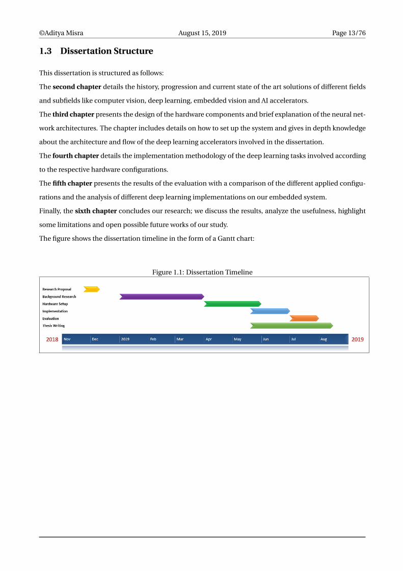
The figure shows the dissertation timeline in the form of a Gantt chart:
Figure 1.1: Dissertation Timeline
©Aditya Misra August 15, 2019 Page 14/76
Chapter 2
State of the Art
2.1 Computer Vision
2.1.1 Definition
Computer vision (CV) is a field of study that deals with development of techniques to help computers gain
an understanding from images and videos. From an engineering outlook, it aims to automate the human
visual system tasks [1][2][3]. It is in general a multidisciplinary field that can be predominantly called a sub-
field of artificial intelligence and involves the use of general algorithms and specialized methods.
Computer vision can be divided into two broad sub-tasks, firstly being implementing methods for acquir-
ing, processing and analyzing images, and secondly, performing the extraction of high-dimensional data
from the real world with an aim to produce relevant numerical or symbolic information [4][5][6][7].
Both the sub-tasks are related to each other in the sense, comprehending the content of the image involves
extraction of symbolic information from image such as, a description, which can be a text description, an
object or a three-dimensional model, etc. using models based on the principles of geometry, physics, statis-
tics, and learning theory [8].
2.1.2 History and Progression
One of the earliest breakthroughs in Computer Vision came in 1959, through the work of two neurophys-
iologists, David Hubel and Torsten Wiesel. Their publication elaborated the core response properties of
visual cortical neurons and their research through experimentation established that simple and complex
neurons existed in the primary visual cortex and as such simple structures like oriented edges were the
starting point of visual processing [9]. In 1959, Russell Kirsch and his colleagues worked on transforming
images into number grids. Their work [10], allows the present processing of digital images in multiple ways.
Lawrence Roberts, in 1963, simplified the visual world to geometric shapes through his elaboration on the

©Aditya Misra August 15, 2019 Page 15/76
process of derivation of 3-Dimensional information about solid objects from their 2-dimensional images
[11].
In 1982, David Marr, built on the ideas of Hubel and Wiesel and established that vision system is hierarchical
with it’s main function being to represent the environment in a 3-Dimensional form such that a person can
interact with it. He introduced a vision framework in which low-level algorithms that detect corners, curves,
edges. etc., were used as the building blocks for a high-level understanding of visual data [12]. In the similar
timeline, Kunihiko Fukushima, a Japanese scientist, built a self-organizing artificial network, Neocognitron,
that consisted of multiple layers whose receptive fields had weight vectors and was successful in recogniz-
ing patterns. His work [13] overcame the limitation of Marr’s work in the sense, it provided a mathematical
modeling for an artificial visual system and defined a learning process for the same.
In 1989, Yann Lecun, used Fukushima’s deep neural network architecture and applied a back-propagation
style learning algorithm to it. Application of his work [14] to the field of character recognition created the
present MNIST dataset. In the late 1990’s the focus of scientists shifted from Marr’s methodology towards
feature-based object recognition. In his work [15], David Lowe implemented a visual recognition system
that consisted of local features which remained unaffected with respect to change in location, rotation and,
partially, illumination. The breakthrough came in 2001, when Paul Viola and Michael Jones were successful
in creating a real-time face detection framework. Their algorithm also consisted of deep learning as, during
image processing, it continuously learned which Haar-like features could help localize faces using boosted
cascade (Adaboost).
With the advancement in the field of Computer Vision, Pascal VOC project was launched in 2006, so as
to provide a benchmark image dataset and standard evaluation metrics for model performance compar-
isons. In 2009, the Deformable Part Model (DPM) was introduced [16] which set great benchmarks in ob-
ject detection tasks. The ImageNet Large Scale Visual Recognition Competition (ILSVRC) was launched in
2010. Overcoming the limitation of Pascal VOC dataset which only provided 20 object categories, ImageNet
dataset provided thousands of object classes. The competition has since become a benchmark for object
detection and classification.
©Aditya Misra August 15, 2019 Page 16/76
2.1.3 Transition towards Deep Learning
Object recognition, detection and classification have always been the fundamental aspects of the Com-
puter vision systems. In computer vision, the scene is broken down into multiple components such that
the computer can easily analyze. Feature Extraction [17], being the first step, is used to identify and extract
the relevant information from the key points in an image. To define practically, it involves examining each
pixel of the image to detect a feature. Scale-invariant feature transform (SIFT) [18] was one of the first im-
plementations of this technology but was not suitable for real time vision systems as it involved complex
floating-point calculations, was computationally intensive and expensive.,
Speeded up robust features (SURF) [19], Histogram of oriented gradients (HOG) [20] and Oriented FAST
and Rotated BRIEF (ORB) [21] were introduced later which were built with the aim of efficient implemen-
tation and combating computationally expensive operations problem of SIFT. SURF overcame the problem
through implementation of a series of mathematical operations like, addition and subtractions for different
frame sizes, easy vectorization and also had low memory requirements. HOG introduced variations to in-
clude different scales for object detection of different sizes, parallel memory access and use of the amount of
overlap between blocks. ORB introduced a combination of binary descriptors and low weight functions for
feature extraction. The success of the former mentioned algorithms in improving the speed and quality of
detection without an increase in computational cost, paved the way for today’s deep learning transforming
frameworks like CNN.
©Aditya Misra August 15, 2019 Page 17/76
2.2 Deep Learning
2.2.1 Definition
Deep learning is a type of machine learning based on artificial neural networks [22]. In deep learning, a
computer is trained to perform human-oriented tasks, like, object detection/classification, speech recogni-
tion, or making predictions. Instead of the traditional way of arranging data and running it through preset
equations, in deep learning we define certain parameters about the data and use multiple layers of process-
ing to train the computer so that it can learn itself by identifying and analysing patterns [23].
The "deep" in "deep learning" refers to the depth (number of layers). "Learning" can be unsupervised,
semi-supervised or supervised [24]. In a deep learning network, the input data is transformed through ev-
ery layer and is converted into a more composite representation. Each layer learns and gradually identifies
which feature to place optimally in which level [25]. The convolution process within Deep Learning helps
in simplifying the feature extraction process. Convolution is a mathematical operation, which maps out an
energy function (the measure of similarity between two images in this case), thus the term Convolutional
Neural Networks [26].
Over the last decade, owing to the success of Alexnet [27] in 2012, there has been a sustained increase in
people worldwide to combine the aspects of classical computer vision local feature detection methods with
the recent deep learning models.
2.2.2 Neural Networks
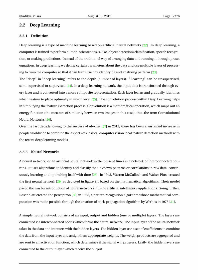
A neural network, or an artificial neural network in the present times is a network of interconnected neu-
rons. It uses algorithms to identify and classify the unknown patterns or correlations in raw data, contin-
uously learning and optimizing itself with time [28]. In 1943, Warren McCulloch and Walter Pitts, created
the first neural network [29] as depicted in figure 2.1 based on the mathematical algorithms. Their model
paved the way for introduction of neural networks into the artificial intelligence applications. Going further,
Rosenblatt created the perceptron [30] in 1958, a pattern recognition algorithm whose mathematical com-
putation was made possible through the creation of back-propagation algorithm by Werbos in 1975 [31].
A simple neural network consists of an input, output and hidden (one or multiple) layers. The layers are
connected via interconnected nodes which forms the neural network. The input layer of the neural network
takes in the data and interacts with the hidden layers. The hidden layer use a set of coefficients to combine
the data from the input layer and assign them appropriate weights. The weight products are aggregated and
are sent to an activation function, which determines if the signal will progress. Lastly, the hidden layers are
connected to the output layer which receive the output.
©Aditya Misra August 15, 2019 Page 18/76
Figure 2.1: Model of an artificial neuron according to McCulloch and Pitts [29]
There are numerous popular neural networks such as, Feed-forward Neural Network, Recurrent Neural Net-
works, Radial basis function Neural Network, Convolutional Neural Networks, etc. Deep Learning for Com-
puter Vision is majorly focused on the use of Convolutional Neural Networks.
2.2.3 Convolutional Neural Networks
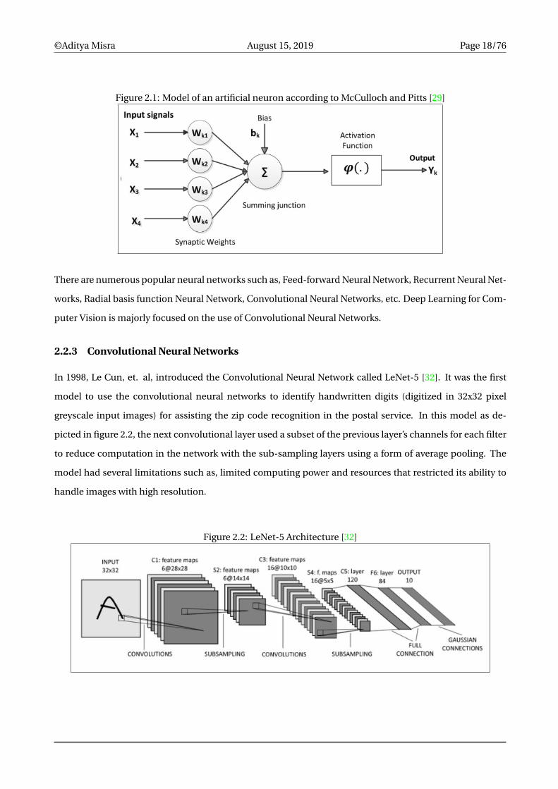
In 1998, Le Cun, et. al, introduced the Convolutional Neural Network called LeNet-5 [32]. It was the first
model to use the convolutional neural networks to identify handwritten digits (digitized in 32x32 pixel
greyscale input images) for assisting the zip code recognition in the postal service. In this model as de-
picted in figure 2.2, the next convolutional layer used a subset of the previous layer’s channels for each filter
to reduce computation in the network with the sub-sampling layers using a form of average pooling. The
model had several limitations such as, limited computing power and resources that restricted its ability to
handle images with high resolution.
Figure 2.2: LeNet-5 Architecture [32]

©Aditya Misra August 15, 2019 Page 19/76
Convolutional Neural Networks are different from the usual neural networks on some architectural aspects
as depicted in figure 2.3. Firstly, the layers in CNN’s have a 3-Dimensional organization, secondly, the neu-
rons of one layer are not connected to every neuron of the next layer but only to some of them and thirdly,
the output is represented as a single vector of probability scores. Training a Convolutional Neural Network
is mathematically complex due to the nature of convolutional operations involved but follows the same pro-
cess of a regular neural network,i.e, trained using gradient descent or back propagation. The functionality
of CNN’s can be divided into two stages:
Figure 2.3: Normal NN vs CNN [33]
Feature Extraction Stage: A series of convolutions and pooling operations are performed by the neural
network in this stage for feature detection. Further elaborating the process, the neural network produces a
feature map through a series of convolutions on the input data using filters/kernels. A convolution is imple-
mented by sliding a filter over input and performing matrix multiplication at each location, finally summing
up the result onto the feature map. Many convolutions are performed on the input with different filters gen-
erating different feature maps, hence, in the end; all the feature maps are taken together and put as he final
output of the convolution layer. Figure 2.4 shows a 2-dimensional convolution operation. In the process
however, the convolution operations are 3-Dimensional with each image having width, height and depth
dimensions. The filter (green square) slides over the input (blue square) and the feature map (red square)
takes the convolution sum as its input. Like other Neural Networks, an activation function (example: ReLU)
Figure 2.4: CNN Operations [34]
©Aditya Misra August 15, 2019 Page 20/76
is also used in a CNN.Two other important terms are Stride and Padding. Stride is the size of the step the
convolution filter moves each time (stride size is usually 1). Padding prevents the shrinkage of the feature
map through addition of a layer of zero-value pixels surrounding the input. Additionally, padding keeps
in check the stride and kernel size, which in turn helps in optimizing the performance. In order to control
over-fitting and reducing the training time, a pooling layer is usually added between the CNN layers, which
helps in reducing the dimensionality.
Therefore, the four important hyper-parameters in case of CNN are: filter count, kernel size, padding and
stride.
The Classification Stage: In this stage, the fully connected layers act as the classifier on the features ex-
tracted in the previous stage. The algorithm predicts the object in the image and a probability is assigned it.
The principle work in this stage involves converting the 3-Dimensional data to 1-Dimensional because the
fully connected layers only accept 1-Dimensional vectors and have access to all the activation functions of
previous layers.
CNN architectures have evolved over the years, however the general design principles still remain the same,
i.e, applying convolutional layers to the input, increasing the number of output feature maps while down-
sampling the spatial dimensions. The classic CNN architectures comprised of simple stacked convolutional
layers, whereas the modern CNN architectures adapt different techniques in the construction of convolu-
tional layers to enhance more efficient learning. These architectures perform rich feature extraction which
facilitate computer vision operations, like, object detection, image classification, image segmentation, etc.
Some of the state of the art image classification architectures include:
AlexNet: Introduced in 2012 by Alex Krizhevsky, et. al, to compete in the ImageNet competition. The gen-
eral network architecture was similar to LeNet-5 but considerably more deeper, with stacked convolutional
layers and more filters per layer [27]. AlexNet reduced the error rate from 26% to 15.3% and performed far
better than the other competitors, thereby, winning the challenge. The success of this model convinced the
computer vision community to delve further into deep learning and start using it for tasks based on com-
puter vision.
GoogLeNet/Inception: Google introduced the Inception network in the 2014 ImageNet challenge. The net-
work model again used a CNN architecture based on LeNet but implemented a novel basic element unit
referred to as an ’inception cell’ [35]. This module was based on a series of several very small convolutions

©Aditya Misra August 15, 2019 Page 21/76
and then doing their subsequent aggregation for reducing the number of parameters. The same researchers
later introduced more efficient alternatives [38] of original inception cell, refined through batch normaliza-
tion at first [36], later refined more in the third iteration through additional factorization ideas [37].
ResNet: Deep residual networks, i.e, deeper networks having more layers were a breakthrough idea, which
enabled the neural network systems to learn more complex functions and result in a better output perfor-
mance. However, they were constrained due to the degradation problem observed in the deep networks.
The researchers concluded that adding more layers resulted into a negative impact on the final output.
Kaiming He et al. introduced ResNet [39] in 2015 to combat the prior mentioned degradation problem.
ResNet consisted of residual blocks, in which the intermediate block layers learned a residual function with
reference to the block input, with each residual block representing itself as an identity function. Using the
methodology, a deep neural network (152 layers) was successfully trained with lower complexity than the
previous counterparts and achieved a much reduced error rate of 3.57%. A later refinement to the original
approach [40] lead to a discovery that the original residual block performed better with more efficient gra-
dient propagation through the network in the training phase. Other researchers later contributed [41] that
the overall capacity of the network can be more efficiently expanded by increasing a network’s width.
SqueezeNet: In 2016, the researchers from Berkeley and Stanford introduced SqueezeNet [42], a model
that achieves the same accuracy as AlexNet but has 50x less weights. The key idea behind SqueezeNet was a
fire module and non-presence of fully connected convolutional layers which helped in greatly reducing the
model size without affecting the accuracy.
MobileNet: In 2017, researchers at Google introduced MobileNet [43], a model that used depth-wise sep-
arable convolutions and outperformed SqueezeNet in cases having a comparable model size. The other
benefit of MobileNet was it’s flexibility, since it was only dependent on two hyper-parameters, therefore, the
architecture could be adapted as per the user’s need.
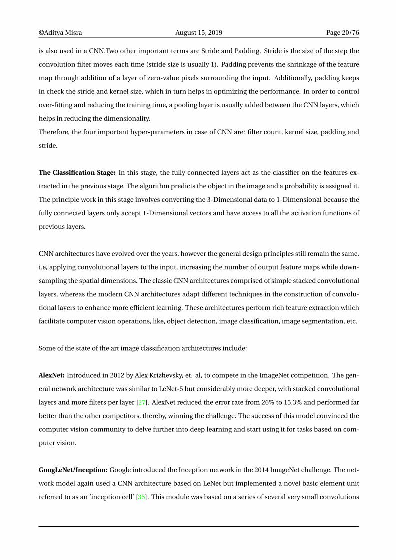
Image classification models detailed previously try to classify images and define them into a single category.
The Object Detection models try to identify the object of interest within the image by drawing a bounding
box around it. The challenge here is the presence of multiple bounding boxes for multiple objects of interest
at a time. This is where a standard CNN followed by a fully connected layer does not work as the length of
the output layer has become variable (multiple object occurrences). The approach in these cases is to use
the object detection algorithms to find fast the different occurrences of the objects of interest within differ-
ent region of interests in the image.
©Aditya Misra August 15, 2019 Page 22/76
Figure 2.5: Image classification, Object detection and Instance segmentation[33]
Some of the state of the art object detection algorithms include:
R-CNN: In 2014, Ross Girshick et al. [44] introduced R-CNN to overcome the limitation of selecting a large
number of regions for object detection which used the selective search method [45]. The selective search
algorithm was used to extract region proposals (region samples) and then further work was performed on
those region proposals.
Fast R-CNN: To reduce the high processing time of R-CNN due to the presence of large number models and
associated region proposals, R. Girshick (2015), introduced Fast R-CNN [46]. The difference in approach
was instead of giving region proposals to CNN as input, an input image was fed to the CNN to produce a
convolutional feature map and then Region of interests were detected using selective search.
Faster R-CNN: Shaoqing Ren et al. [47] introduced Faster R-CNN which followed the methodology of Fast
R-CNN till the point of feature map generation. In the last step, it used Region Proposal Network (RPN), a
separate network, to directly learn and generate region proposals, predict bounding boxes and detect ob-
jects, thus eliminating the need of selective search algorithm .
You Only Look Once (YOLO): J. Redmon et al., 2016 introduced YOLO [48] and it differed from the prior
object detection algorithms in the initial approach itself. YOLO was a simple model that used a single con-
volutional network to predict the bounding boxes and their class probabilities in a single evaluation, thus
allowing real-time predictions.
Single-Shot Detector (SSD): W. Liu et al. introduced SSD [49] to predict the bounding boxes and the re-
spective class probabilities in a single shot. Very similar in approach to the YOLO model, the difference in

©Aditya Misra August 15, 2019 Page 23/76
the architecture was the use of extra feature layers in SSD for increasing the number of relevant bounding
boxes.
Region-based Fully Convolutional Network (R-FCN): J. Dai and al. (2016) introduced R-FCN [50], a sin-
gle model consisting only of convolutional layers, simultaneously taking into account the object detection
(location invariant) and its position (location variant), thus, allowing complete back-propagation for train-
ing and inference.
©Aditya Misra August 15, 2019 Page 24/76
2.3 Embedded Computer Vision
2.3.1 Definition
“Embedded Vision” refers to the practical use of computer vision in machines that understand their envi-
ronment through visual means [51]. Elaborating in simpler terms, embedded vision refers to the integration
of a camera and processing board. Since its inception, the computer vision field has seen the application
of intelligent algorithms and digital processing in order to extract useful information from the images or
videos. Historically, the vision setup consisted of a separate camera and a PC, considered both large and
expensive. Evolving over the time, both cameras and PC’s shrunk in size and became affordable, the proces-
sors became powerful, therefore, making it possible to integrate practical computer vision capabilities into
the embedded systems [52]. Embedded vision systems present various advantages, such as, compact size,
lightweight, low cost and low energy consumption in their respective applications [53].
2.3.2 Embedded Vision Systems
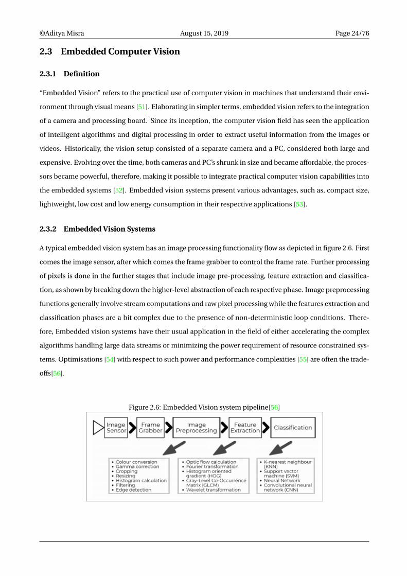
A typical embedded vision system has an image processing functionality flow as depicted in figure 2.6. First
comes the image sensor, after which comes the frame grabber to control the frame rate. Further processing
of pixels is done in the further stages that include image pre-processing, feature extraction and classifica-
tion, as shown by breaking down the higher-level abstraction of each respective phase. Image preprocessing
functions generally involve stream computations and raw pixel processing while the features extraction and
classification phases are a bit complex due to the presence of non-deterministic loop conditions. There-
fore, Embedded vision systems have their usual application in the field of either accelerating the complex
algorithms handling large data streams or minimizing the power requirement of resource constrained sys-
tems. Optimisations [54] with respect to such power and performance complexities [55] are often the trade-
offs[56].
Figure 2.6: Embedded Vision system pipeline[56]

©Aditya Misra August 15, 2019 Page 25/76
Different types of processors used for performing the embedded vision tasks include:
Central Processing Unit (CPU): A CPU, is an electronic circuitry residing inside a computer that consists
primarily of an Arithmetic Logic Unit, processor registers and a control unit, which facilitates the execution
of instructions. The increasing popularity and adoption of computer vision techniques in various fields,
such as, robotics, medicine, etc. together with a need for educating students to gain expertise in both these
fields (electronics and vision) led to the introduction of various CPU based single board platforms, such
as, Raspberry-Pi [57], Arduino [58], Nvidia Jetson [59], etc. While Otterness et.al [60], evaluated the effec-
tiveness of NVIDIA Jetson TX in supporting the real-time computer-vision workloads, [61] shows the vision
tasks performed on a Raspberry-Pi to demonstrate the effective embedded image processing and Eisenberg
et al. developed LilyPad, a construction kit to design textile artifacts using Arduino [62].
Graphic Processing Unit (GPU): A GPU is a specialized electronic circuit capable of rapid alteration and
manipulation of memory for accelerated creation of images in a frame. They have a highly parallel struc-
ture, which makes them faster than the CPU’s in case of processing algorithms that use large blocks of data
[63]. GPUs are used in embedded systems, personal computers, game consoles and also in combination
with programming models like OpenCL on mobile devices. A sample of GPU capabilities has been demon-
strated in works of Rister et al [64], Andargie et.al [65] and Szegedy et. al [66]. While in [64], an implementa-
tion of SIFT on GPU is shown, [65] presents a two fold up speedup in object detection algorithm using GPU
over a GPP and [66] presents a research on scaling up of convolutional networks based on a GPU enabled
architecture.
Application Specific Integrated Circuits (ASIC): To combat the problems of slow processing, high com-
putational cost and increasing the usefulness of vision based applications and systems in real-time appli-
cations, the researchers introduced the use of ASIC for producing dedicated solutions. Some of the popular
works include the use of deep networks [67] for combating high computational costs in models understand-
ing the visual, audio and video content, use of scalable and low power processor in [68] for deep learning
on mobile and [69] for performing lossless data compression.
©Aditya Misra August 15, 2019 Page 26/76
Field Programmable Gate Array (FPGA): FPGA’s provide an advantage of independent configurability over
CPU’s and GPU’s. They are a type of integrated circuits that are user/designer configurable and contain an
array of programmable logic blocks, which can be configured to perform complex functions or simple gate
logic and reconfigurable interconnects that wire the logic blocks together. They are successfully used in
embedded computer vision due to their faster rate of processing owing to their parallel and pipelined ar-
chitecture. In [54], the authors show the functionality of vision system pipeline and the associated parallel
execution in various forms (task and data). The parallel structure of FPGA’s has also been successfully ex-
ploited in the works of [70][71] for Neural network based reinforcement learning acceleration and in [72][73]
for feature classification using Convolutional Neural Networks.

©Aditya Misra August 15, 2019 Page 27/76
2.4 Deep Learning on the Edge
2.4.1 Resurgence of Edge Computing
Edge computing, a form of distributed computing is a concept that brings computer data storage closer to
the location where it is needed [74]. It is not a new concept with its roots dating back to 90’s, first of its
implementation example being the launch of a content delivery network by Akamai aimed to resolve web
congestion. Recent trends in cloud computing and artificial intelligence (especially machine learning) has
led to its resurgence. However, it continues to address the same problem of proximity, trying to reduce the
bandwidth, latency and overhead of the centralized data center by bringing the computer workload closer
to the consumer [75].
At present, with the progression of semiconductor technologies in terms of increased speeds, shrinking ge-
ometries, and low power consumption, and the introduction of System-on-Chip (SoC) devices, billions of
edge devices are being deployed in various application sectors such as, automotive, medical, industrial,
security and surveillance, etc. These edge devices consist of various types of sensors, which generate hu-
mongous amounts of data of various types such as, images, video, speech and other non-imaging data,
which is transmitted back to cloud. Several challenges exist in this aspect, such as, round trip delays in
transmission of data impacting the latency of the applications, security and privacy needs for critical data,
therefore, there is a need to develop next generation of edge devices which come with intelligent decision
making capabilities.
2.4.2 Edge over Cloud
With the increasing popularity of edge computing over cloud computing [76], it is being predicted that for-
mer will replace the latter at some point in the future. However, the cloud computing has its own target
areas where the edge computing usually fall short [77]. Still edge computing solves many challenges in-
volved with the cloud, some of them being:
Latency: Edge computing focuses on resolving the proximity issue, which directly addresses the latency
issue. In the on-device approach, an immediate action is taken as soon as the critical data is encountered
and only the remaining non-useful data is sent over the network. That is important for applications need-
ing instantaneous inference and are latency-sensitive, such as autonomous vehicles, where every second is
critical. As such, there has been an introduction of on-board compute devices to perform inference on the
edge [78].
©Aditya Misra August 15, 2019 Page 28/76
Bandwidth: The distributed approach of edge computing helps in combating the need of increasing band-
width. With the data processing being done at the collection point and only specific data in need of being
stored being sent to the cloud network, the network load is greatly reduced, thus decreasing the bandwidth.
Edge computing is also makes scaling more efficient as it provides the option of connecting large number
of devices to the same network.
Security and Reliability: Edge networking helps in enhancing the security in two key ways. First being
the aspect of presence of less data on cloud as most of the data is processed at the collection point, so less
threat of a data breach/leak. Second being the presence of a decentralized architecture that is much harder
to bring down than a centralized one. Edge computing also aids in outage reduction, better intermittent
connectivity, avoiding unplanned server downtime as it solely does not rely on the cloud. The distributed
node network provides an assurance that even if one of the edge devices (here, a node) fails; its neighbor
can take over temporarily.
Support for Online/Continuous Learning: Edge Devices are quite useful for Reinforcement Learning, as
they can aid in data collection for Online Learning and help in parallel simulation of large number of
episodes for the model to learn. Optimization techniques such as, Asynchronous SGD, can be used to train
a single model in parallel in whole or partial edge network [79].
Increased Cost Effectiveness: The cloud services are costly in the long run especially if they run contin-
uously for long periods. Instead, they can be replaced with a set of edge devices, which can provide on
device inference.

©Aditya Misra August 15, 2019 Page 29/76
2.4.3 Bringing Deep Learning to the Edge Devices
Since its inception, Deep Learning brings along with it the need of powerful CPUs and GPUs, Large Cloud
infrastructure, heavy software packages and frameworks for its fruitful execution. These heavy frameworks
in turn result in heavy computations and longer inference run times, which makes the application of Deep
Learning in edge devices for real-time inferences infeasible. Therefore, a big challenge at present is to fit the
Deep Learning models into the compact, low power consuming and minimal storage requiring next gener-
ation edge devices, which will support the quick real-time inferences. Some of the present ways to tackle
the problem include:
Parameter Efficient Neural Networks: A big challenge with neural networks was their enormous size, which
made it difficult to fit them into compact edge devices. The researchers were motivated by this aspect and
worked on minimizing the size of the neural networks without compromising on the accuracy. This re-
sulted in two popular efficient neural networks at present, the SqueezeNet [42] and the MobileNet [43].
While SqueezeNet incorporates techniques like, late down sampling, filter count reduction and use of fire
modules to get high performance at low parameter count, the MobileNet uses the concept of depth wise
convolutions.
Pruning, Quantization and Distillation: Researchers at Google introduced Learn2Compress (architecture
depicted in figure 2.7) [80] that involves use of several state-of-the-art techniques for compressing and op-
timizing neural network models to assist in building up custom on-device Machine Learning and Deep
Learning models [81]. Some of the popular techniques include:
Figure 2.7: Learn2Compress for automatically generating on-device ML models[80]
Pruning to reduce the model size by removing the benign neurons in the trained network not contributing
to the final accuracy (e.g.low-scoring weights). This can be very effective in obtaining a size reduction (up
to 2x factor) especially for on-device models involving sparse inputs or outputs, while retaining 97% of the
accuracy.
©Aditya Misra August 15, 2019 Page 30/76
Quantization for reducing the precision of the involved neural network parameters. Instead of the usual
32-bit float values, edge devices can be designed to work on 8-bit values or less. Reduction in precision im-
proves the inference speed, reduces the power consumption and reduces the size of the model (by a factor
of 4x in the case described before).
Joint training and distillation to teach smaller networks (on-device models) using a larger ‘teacher’ net-
work (user provided model). When combined further with transfer learning, it becomes a powerful way of
reducing model size with minimal loss in accuracy.
Optimized Microprocessor Designs: As an alternative to scale down neural networks to fit in the edge
devices, the researchers are also working to scale up the performance of the microprocessors. Different
approaches are possible in this aspect and as such, different products exist, such as, Nvidia Jetson, which
uses a GPU on microprocessor, Google AIY kit and Intel’s Neural Computing Stick that internally use Vision
Processing Units (VPUs) and Nvidia V100 which uses custom ASICs to accelerate the performance.

©Aditya Misra August 15, 2019 Page 31/76
2.5 AI Accelerators
2.5.1 Definition and History
AI accelerators are a type of microprocessors built with the purpose of providing hardware acceleration for
artificial intelligence applications. General applications areas include machine vision,internet of things,
robotics and deep learning. They are generally multi-core processors ingrained with capabilities like han-
dling and performing low-precision arithmetic, in-memory computing, high degree of parallel processing,
etc.
In the 90’s there were various instances of exploring the field of accelerators. Attempts for creation of parallel
systems for neural network simulations, trial for accelerating the optical character recognition using digital
signal processors, exploration of Field Programmable Gate Array (FPGA) based accelerators for training and
inferencing and introduction of Heterogeneous System Architecture. In the later years, Graphical Process-
ing Units (GPUs) and FPGAs were explored, where the former became the most popular choice for handling
of AI related operations the latter due to its re-configurability property, made it easier for the hardware,
frameworks and software to evolve alongside each other with the changing Deep Learning frameworks. At
present, there is a rise of AI accelerator Application Specific Integrated Circuits (ASICs) and System On Chip
(SOCs) dedicated to specific field of operation like computer vision, etc.
2.5.2 Rising Need for Deep Learning Accelerators
The progression of artificial intelligence (AI) in the last decade was mainly aided by the GPUs, even if they
were not initially built keeping in mind the neural network deployments that happened in the future. GPUs
gave the Deep Learning algorithms a significant boost in performance and made training of the neural
networks to cater to the real world problems possible. As the AI demand grows, more chips that are powerful
are need for computing answers (inference) from large data sets (training). Until a recent few years, data
centers were the key players for training and inferencing of the models, however with the shifting trend
towards the edge, the training portion may be handled by the data center in the future but most of the
inferencing will be done on the edge. Therefore, at present, a new breed of AI accelerators is unfolding,
having characteristics like, high-speed memory, fast data access and multi-node scaling [82]. Different types
of applications require different levels of Deep Learning inferencing to solve different complex problems
and it is not feasible or practical to develop different Deep Learning edge solutions for different applications.
As such, there is a need to develop highly integrated and configurable System on Chip (SOC) solutions with
embedded Deep Learning hardware accelerators for fulfilling the Deep Learning inference needs of edge
devices catering to a wide range of applications.
©Aditya Misra August 15, 2019 Page 32/76
2.5.3 Current Deep Learning Accelerators
GPU based accelerators: Over the time, GPUs have become standard for various artificial intelligence (AI)
applications, such as, face, object detection/recognition, data mining, etc. GPUs offers various advantages
such as, variety of hardware selections, a high-performance throughput and high computing power [83].
Some of the popular GPA based accelerators include:
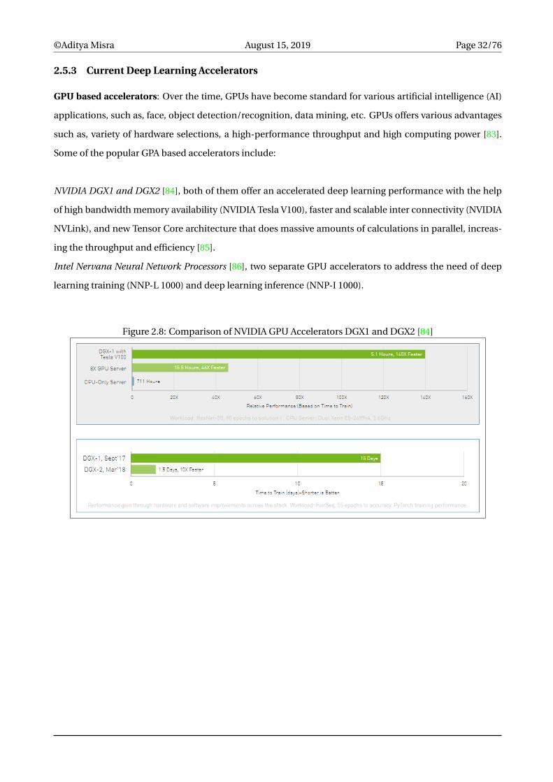
NVIDIA DGX1 and DGX2 [84], both of them offer an accelerated deep learning performance with the help
of high bandwidth memory availability (NVIDIA Tesla V100), faster and scalable inter connectivity (NVIDIA
NVLink), and new Tensor Core architecture that does massive amounts of calculations in parallel, increas-
ing the throughput and efficiency [85].
Intel Nervana Neural Network Processors [86], two separate GPU accelerators to address the need of deep
learning training (NNP-L 1000) and deep learning inference (NNP-I 1000).
Figure 2.8: Comparison of NVIDIA GPU Accelerators DGX1 and DGX2 [84]

©Aditya Misra August 15, 2019 Page 33/76
FPGA based accelerators: With the industry evolving, FPGAs are now competing with the GPUs for im-
plementing AI solutions. Microsoft Research’s Catapult Project claimed that using FPGAs could be as much
as 10 times more power efficient compared to GPUs [87]. A popular example of the FPGA based accelerator
is the recent Project Brainwave unveiled by Microsoft, which is a high performance, distributed system hav-
ing soft Deep Neural Network (DNN) systems synthesized onto Intel’s Stratix FPGAs that provides real time
AI with ultra-low latency [88].
Figure 2.9: Microsoft’s Project Brainwave powered by FPGAs [88]
ASIC based accelerators: Compared to FPGAs, Application Specific Integrated Circuits (ASICs) offer higher
efficiency of the Deep Learning algorithms, less complex programmable logic and reduced hardware design
cost. Although the FPGAs reduce the computing power consumption, their speed is 4-5x times lower than
ASICs [89]. Other reasons for a rapid rise of ASICs for supporting edge based AI include reduced network
overhead, reduced off-chip memory access, support for low power convolutional operations with reduced
processing times [90][91][92]. Modern ASICs often include entire microprocessors, memory blocks and
other large building blocks, often termed as System on Chip (SOC). A primary example of that being intro-
duction of a Vision Processing Unit (VPU) – Movidius Myriad X by Intel to accelerate machine vision tasks
[93].
Another prominent example of ASIC based edge accelerators are neural computing sticks, which compli-
ment the SOC solutions in accelerating the deep learning inference. The most popular currently being
Movidius Neural Computing Stick (NCS), a small USB device consisting of Myriad VPU and hardware accel-
erators for neural network inferencing, introduced by Intel. It is being used for building applications that
support vision tasks such as, Embedded Object Detection and Recognition [94], Emotion Recognition [95],
etc. Google has also recently launched EdgeTPU [96], an open, end-to-end infrastructure for deploying AI
solutions.
©Aditya Misra August 15, 2019 Page 34/76
Chapter 3
Design
3.1 Raspberry Pi
3.1.1 Overview
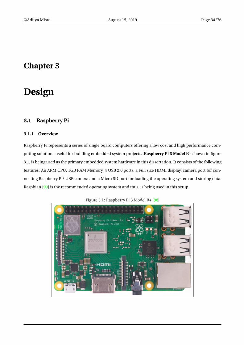
Raspberry Pi represents a series of single board computers offering a low cost and high performance com-
puting solutions useful for building embedded system projects. Raspberry Pi 3 Model B+ shown in figure
3.1, is being used as the primary embedded system hardware in this dissertation. It consists of the following
features: An ARM CPU, 1GB RAM Memory, 4 USB 2.0 ports, a Full size HDMI display, camera port for con-
necting Raspberry Pi/ USB camera and a Micro SD port for loading the operating system and storing data.
Raspbian [99] is the recommended operating system and thus, is being used in this setup.
Figure 3.1: Raspberry Pi 3 Model B+ [98]

©Aditya Misra August 15, 2019 Page 35/76
3.1.2 Setup
List of Components
The following components are needed for our setup:
• A minimum 2.5 amps micro USB power supply.
• A Storage Disk (SD) Card (16 or 32 GB) to store all files and the operating system.
• A keyboard and a mouse.
• An HDMI Cable.
• A computer screen.
• A USB camera.
SD Card Setup
New Out Of Box Software (NOOBS) operating system installation manager is the simplest way to install the
Raspbian operating system on the SD Card (using a computer and SD Card Reader).
Following are the steps to install the operating system on the SD card:
• Download the zip file for NOOBS installation available at the Raspberry Pi website [99].
• Format the SD card using SD Formatter.
• Extract NOOBS from the zip archive.
• Copy the extracted files to the SD card.
After finishing the operating system installation, insert the SD card into the Raspberry Pi. The final compo-
nent connection setup before starting the Raspberry Pi is shown in figure 3.2.
3.1.3 Starting the Raspberry Pi
After connecting all the components and setting up the SD card with the operating system, the following
steps are carried out to start up the Raspberry Pi:
• Connect the 2.5 amps micro USB power supply to the power port, a red LED light should light up on
the Raspberry Pi. The Raspbian desktop will appear on the computer screen as shown in figure 3.3.
• Follow the steps of Welcome to Raspberry Pi application for completing the initial setup (includes
setting up of time zone, Wi-Fi setup and user profile completion).
• Reboot for finishing the setup.

©Aditya Misra August 15, 2019 Page 36/76
Figure 3.2: Component Connection Setup [98]
Figure 3.3: Raspberry Pi Desktop start screen

©Aditya Misra August 15, 2019 Page 37/76
3.2 Intel Movidius Neural Computing Stick
3.2.1 Overview
Intel Movidius Neural Computing Stick (NCS) is a low power deep learning accelerator in the form of a USB
stick as shown in figure 3.4, consisting of high performance Intel Myriad Vision Processing Unit (VPU). Myr-
iad VPUs are specially designed for handling the computer vision and associated deep learning tasks. While
Myriad is essentially a System-on-Chip (SoC) board, Intel has extended the same technology to Movidius
NCS, which can be used to prototype, tune, validate and deploy deep neural networks on the edge devices
such as Raspberry Pi. Since its launch in 2017, two versions of NCS devices are available in the market
namely, Intel NCS 1 and Intel NCS 2, both of them are being incorporated in this dissertation.
The Intel NCS 1 consists of the Intel Movidius Myriad 2 VPU and the Intel NCS 2 consists of the Intel Mo-
vidius Myriad X VPU that includes two Neural Compute Engines (NCE) for accelerating deep learning in-
ferences at the edge and responding in real time. Intel Movidius Neural Compute SDK (NCSDK) [102], as-
sociated with the Intel NCS 1, is the primary software toolkit consisting of software tools and API. The Intel
NCS 2 on the other hand comes with the Open Visual Inference Neural Network Optimization (OpenVINO)
toolkit [100], a unified platform for model optimization and inferencing; The Intel NCS 2 is not compatible
with the NCSDK, while Intel NCS 1 is compatible with the OpenVINO toolkit. Both the NCS devices and their
associated methodologies for implementing deep learning inferencing on the edge have been incorporated
in this dissertation and are discussed in further subsections.
Figure 3.4: Intel Movidius Neural Computing Stick [97]

©Aditya Misra August 15, 2019 Page 38/76
3.2.2 Intel Movidius Neural Compute SDK (Intel Movidius NCSDK)
Overview and Architecture
The Intel Movidius NCSDK consists of two components as shown in figure 3.5, an NC Toolkit, which consists
of a Profiler, Checker and Compiler, and an NC API. In the NC Toolkit, the Profiler is used to get a better
insight of the deep neural network’s complexity, execution time and bandwidth, the Checker is used to run
an inference on the NCS and compare the result with that of the trained network and the Compiler is used
to convert the deep neural network into a binary graph file that can be used by the NC API. Each component
of the NC Toolkit corresponds to a command line tool (Profiler - mvNCProfile, Checker - mvNCCheck and
Compiler - mvNCCompile) which are discussed in the figure 3.6.
Figure 3.5: Intel Movidius NCSDK components [97]
Figure 3.6: NC Toolkit command line tools [97]
The NC API is then used to build applications that can be deployed on the edge devices with accelerated
deep learning inferencing. The complete architecture of the NCSDK workflow is shown in the figure 3.6.
©Aditya Misra August 15, 2019 Page 39/76
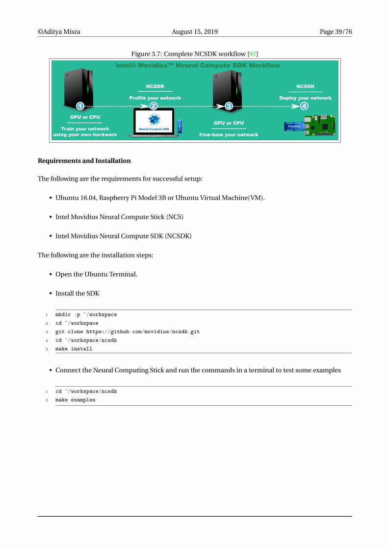
Figure 3.7: Complete NCSDK workflow [97]
Requirements and Installation
The following are the requirements for successful setup:
• Ubuntu 16.04, Raspberry Pi Model 3B or Ubuntu Virtual Machine(VM).
• Intel Movidius Neural Compute Stick (NCS)
• Intel Movidius Neural Compute SDK (NCSDK)
The following are the installation steps:
• Open the Ubuntu Terminal.
• Install the SDK
1 mkdir -p ~/workspace2 cd ~/workspace3 git clone https://github.com/movidius/ncsdk.git4 cd ~/workspace/ncsdk5 make install
• Connect the Neural Computing Stick and run the commands in a terminal to test some examples
1 cd ~/workspace/ncsdk2 make examples

©Aditya Misra August 15, 2019 Page 40/76
3.2.3 OpenVINO toolkit
Overview
OpenVINO is a toolkit based on Convolutional Neural Networks (CNN) that facilitates fast-track develop-
ment of computer vision algorithms and deep learning neural networks into vision applications, and en-
ables their easy heterogeneous execution across hardware platforms. OpenVINO consists of a Deep Learn-
ing Deployment Toolkit (DLDT) and contains optimized functions for OpenCV (Open Source Computer Vi-
sion Library) [107], OpenCL (Open Computing Language) [110] etc. The complete architecture is as shown
in figure 3.8.
Primary benefits of OpenVINO include:
• CNN-based deep learning inference on the edge using a common API and several pretrained models.
• Heterogeneous execution support across Intel hardware platforms such as, an Intel CPU, Intel Inte-
grated Graphics, Intel FPGA, Intel Movidius Neural Compute Stick (1 and 2), and Intel Movidius VPUs.
• Presence of easy ready to use library of computer vision functions and pre-optimized kernels that
speeds up the time-to-market of applications.
• Consists of optimized functions for computer vision standards, such as, OpenCV, OpenCL,etc.
Figure 3.8: OpenVINO Architecture [100]

©Aditya Misra August 15, 2019 Page 41/76
Deep Learning Deployment Toolkit (DLDT) Architecture
The DLDT has two components, a Model Optimizer (shown in figure 3.9) and an Inference Engine (shown
in figure 3.10).
Model Optimizer: A Python based cross-platform command-line tool that works on multiple operating
systems (Windows, Linux and MacOS) and is used for two primary tasks:
• Importing trained models trained on popular frameworks, such as Caffe, TensorFlow, Apache MXNet,
and Open Neural Network Exchange (ONNX).
• Preparing them for optimal execution with the Inference Engine through conversion of models into
an intermediate representation (IR) format from Intel.
Figure 3.9: Model Optimizer Architecture [100]
Inference Engine: An execution engine that uses a common API to deliver high performance inference
solutions on different hardware platforms (CPU, GPU, VPU, or FPGA). It is capable of running different
neural network layers on different target platforms, thereby optimizing the workloads for enhancing the
performance.
Figure 3.10: Inference Engine Architecture [100]
©Aditya Misra August 15, 2019 Page 42/76
3.3 Neural Networks
3.3.1 Overview
The NCSDK supports only GoogLeNet, AlexNet, SqueezeNet for Image Classification and MobileNet-SSD
and YOLO for Object Detection. Therefore, for a proper comparison between Intel NCS 1 using NCSDK
and Intel NCS 2 using OpenVINO, the GoogLeNet, AlexNet and SqueezeNet architectures are being used
for Image Classification and MobileNet-SSD is being used over YOLO for object detection as it provides
a better accuracy and framerate [100]. The Neural Compute Application Zoo (NCAppZoo) [101] contains
these pre-trained deep neural networks, their weights can be leveraged and the models can be fine-tuned
and optimized to suit own custom requirements. The same approach has been followed in this work’s setup.
Datasets
ImageNet [103] is an image dataset containing about 20,000 categories with each category consisting of
several hundred images, which are hand-annotated by the project to indicate the types of objects pictured.
The GoogLeNet, AlexNet, and SqueezeNet networks being used have been trained on the ImageNet dataset.
COCO [104] is dataset having 80 object categories and around 330k images, useful for large-scale object
detection. The MobileNet-SSD network being used has been trained on the COCO dataset.

©Aditya Misra August 15, 2019 Page 43/76
3.3.2 AlexNet
The AlexNet [27] has a relatively simple architecture as shown in figure 3.11, consisting of eight layers (5
convolutional layers and 3 fully connected layers). ReLU activation function is applied after all the convolu-
tional and fully connected layers except the output layer where a normalized exponential function (softmax)
is applied. Local normalization is applied after first and second convolutional layers; Max Pooling (Over-
lapping) is applied after first, second and fifth convolutional layers and lastly Dropout is applied after layers
first and second fully connected layers. The first convolutional layer consists of 11x11 filters at stride 4 with
zero padding; the second convolutional layer consists of 5x5 filters at stride 1 with padding as two; the third,
fourth and fifth convolutional layers are the same with 3x3 filters at stride 1 with padding as one. All the Max
Pool layers consist of 3x3 filters at stride 2.
Figure 3.11: AlexNet Architecture [27]
The key features of this architecture are:
1. Use of ReLU to add non-linearity that accelerates the speed without compromising on existing accu-
racy.
2. Use of Dropout instead of regularization for combating the problem of over-fitting.
3. Use of Overlap Pooling for reducing the network size and therefore the error rate.
Because the network resided on two GPUs, it is split in two parts that communicate only partially, half the
feature maps on each GPU. The first, second, fourth and fifth convolutional layers have connections with
feature maps on the same GPU, while the third convolutional layer and all the fully connected layers have
connections with all the feature maps in the preceding layer and can communicate between GPUs.

©Aditya Misra August 15, 2019 Page 44/76
3.3.3 GoogLeNet
The Inception (GoogLeNet) network model uses a similar CNN architecture based on LeNet but consists of a
novel basic element unit referred to as an ’inception module’ [35]. The architecture as shown in figure 3.12,
consists of a 22 layer deep CNN, using 1x1 convolutions for reducing the input channel depth, 1x1, 3x3, 5x5
filters for each inception cell to extract features at different scales, MaxPooling and Padding for preserving
dimensions for proper concatenation of output at later stages. A local network topology is designed where
the inception modules are stacked on top of each other.
Figure 3.12: GoogLeNet architecture [35]
As depicted in the figure 3.13, in a Naïve inception module, parallel filter operations are applied on the input
from the previous layer (Multiple sizes of Convolution - 1x1, 3x3, 5x5 and Pooling – 3x3) and filter outputs
are concatenated depth wise. This results in a much computationally expensive process with high magni-
tude of operations. Therefore, In GoogLeNet, in order to reduce the computation, 1×1 convolution is used
as a dimension reduction module.
Figure 3.13: Inception module architecture [35]
The reduction of computation bottleneck facilitates the increase of depth and width of the network. Further,
instead of using the fully connected layers as in the previous architectures, GoogLeNet uses global average
pooling at the end of the network, which helps in increasing the accuracy of the network. Certain interme-
diate softmax branches are also used in the middle that help combat the vanishing gradient issue and also
provide regularization.
©Aditya Misra August 15, 2019 Page 45/76
3.3.4 SqueezeNet
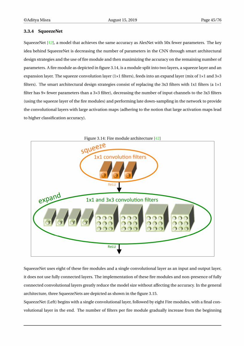
SqueezeNet [42], a model that achieves the same accuracy as AlexNet with 50x fewer parameters. The key
idea behind SqueezeNet is decreasing the number of parameters in the CNN through smart architectural
design strategies and the use of fire module and then maximizing the accuracy on the remaining number of
parameters. A fire module as depicted in figure 3.14, is a module split into two layers, a squeeze layer and an
expansion layer. The squeeze convolution layer (1×1 filters), feeds into an expand layer (mix of 1×1 and 3×3
filters). The smart architectural design strategies consist of replacing the 3x3 filters with 1x1 filters (a 1×1
filter has 9× fewer parameters than a 3×3 filter), decreasing the number of input channels to the 3x3 filters
(using the squeeze layer of the fire modules) and performing late down-sampling in the network to provide
the convolutional layers with large activation maps (adhering to the notion that large activation maps lead
to higher classification accuracy).
Figure 3.14: Fire module architecture [42]
SqueezeNet uses eight of these fire modules and a single convolutional layer as an input and output layer,
it does not use fully connected layers. The implementation of these fire modules and non-presence of fully
connected convolutional layers greatly reduce the model size without affecting the accuracy. In the general
architecture, three SqueezeNets are depicted as shown in the figure 3.15.
SqueezeNet (Left) begins with a single convolutional layer, followed by eight Fire modules, with a final con-
volutional layer in the end. The number of filters per fire module gradually increase from the beginning
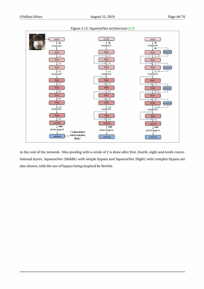
©Aditya Misra August 15, 2019 Page 46/76
Figure 3.15: SqueezeNet architecture [42]
to the end of the network. Max-pooling with a stride of 2 is done after first, fourth, eight and tenth convo-
lutional layers. SqueezeNet (Middle) with simple bypass and SqueezeNet (Right) with complex bypass are
also shown, with the use of bypass being inspired by ResNet.
©Aditya Misra August 15, 2019 Page 47/76
3.3.5 MobileNet-SSD
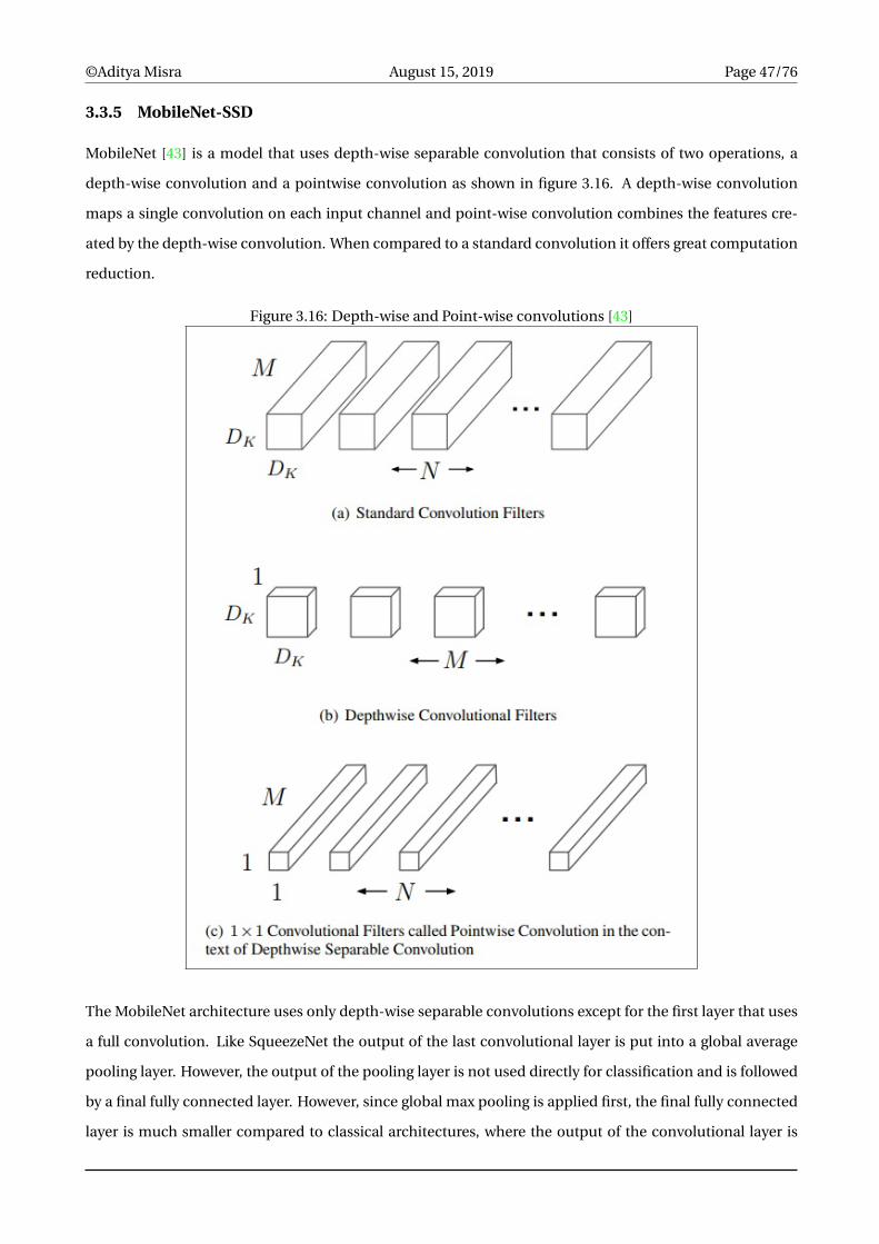
MobileNet [43] is a model that uses depth-wise separable convolution that consists of two operations, a
depth-wise convolution and a pointwise convolution as shown in figure 3.16. A depth-wise convolution
maps a single convolution on each input channel and point-wise convolution combines the features cre-
ated by the depth-wise convolution. When compared to a standard convolution it offers great computation
reduction.
Figure 3.16: Depth-wise and Point-wise convolutions [43]
The MobileNet architecture uses only depth-wise separable convolutions except for the first layer that uses
a full convolution. Like SqueezeNet the output of the last convolutional layer is put into a global average
pooling layer. However, the output of the pooling layer is not used directly for classification and is followed
by a final fully connected layer. However, since global max pooling is applied first, the final fully connected
layer is much smaller compared to classical architectures, where the output of the convolutional layer is
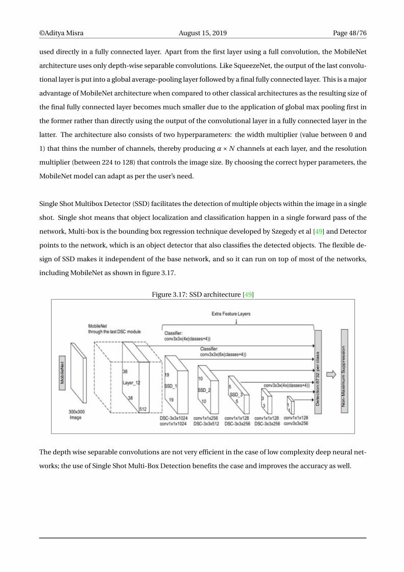
©Aditya Misra August 15, 2019 Page 48/76
used directly in a fully connected layer. Apart from the first layer using a full convolution, the MobileNet
architecture uses only depth-wise separable convolutions. Like SqueezeNet, the output of the last convolu-
tional layer is put into a global average-pooling layer followed by a final fully connected layer. This is a major
advantage of MobileNet architecture when compared to other classical architectures as the resulting size of
the final fully connected layer becomes much smaller due to the application of global max pooling first in
the former rather than directly using the output of the convolutional layer in a fully connected layer in the
latter. The architecture also consists of two hyperparameters: the width multiplier (value between 0 and
1) that thins the number of channels, thereby producing α×N channels at each layer, and the resolution
multiplier (between 224 to 128) that controls the image size. By choosing the correct hyper parameters, the
MobileNet model can adapt as per the user’s need.
Single Shot Multibox Detector (SSD) facilitates the detection of multiple objects within the image in a single
shot. Single shot means that object localization and classification happen in a single forward pass of the
network, Multi-box is the bounding box regression technique developed by Szegedy et al [49] and Detector
points to the network, which is an object detector that also classifies the detected objects. The flexible de-
sign of SSD makes it independent of the base network, and so it can run on top of most of the networks,
including MobileNet as shown in figure 3.17.
Figure 3.17: SSD architecture [49]
The depth wise separable convolutions are not very efficient in the case of low complexity deep neural net-
works; the use of Single Shot Multi-Box Detection benefits the case and improves the accuracy as well.

©Aditya Misra August 15, 2019 Page 49/76
Chapter 4
Implementation
Following the design laid out in Chapter 3, in this chapter, the implementation details of Image classification
and Real-time object detection done using the Intel Movidius Neural Computing Sticks on the Raspberry Pi
are discussed. Furthermore, the methodologies to derive the appropriate deep learning inferences from
the respective setups are also discussed. The Neural Compute Application Zoo (NCAppZoo) [101] contains
the pre-trained deep neural networks required for our experiments that can be fine-tuned and optimized
to suit own custom requirements. The weights of our respective neural networks for Image Classification
(AlexNet, GoogLeNet and SqueezeNet) and Real Time Object Detection (MobileNet-SSD), are being lever-
aged instead of training them from the scratch. The deep learning models are implemented using Caffe and
the implementation code for accessing the Neural Computing Stick, performing the computer vision tasks
and deriving the deep learning inferences from the same has been written in Python 3.5. The links to the
implementation code and associated videos are provided in the attached CD.
4.1 Overview
The Intel Movidius NCSDK can be used in two modes, a Full SDK Mode and an API only mode. In the
API only mode we install only the API framework on the system and applications are developed without the
toolkit. In the Full SDK mode, the full toolkit and API framework is installed on the system with the profiling,
validation and compiling of the neural networks into a binary graph file also done on the system. We will
be using the API-only mode installation on the Raspberry-Pi as the Full SDK installation and execution gets
very complex and overloads the processor of our low powered embedded board which in turn can impact
the output results. In parallel, we will be using Full SDK installation on separate Linux machine, where we
will generate a graph file by compiling the neural networks involved. The OpenVINO toolkit will be used
in a combination with the Movidius VPU, which will be used to perform the deep learning inference as it is
optimized and designed for the same.
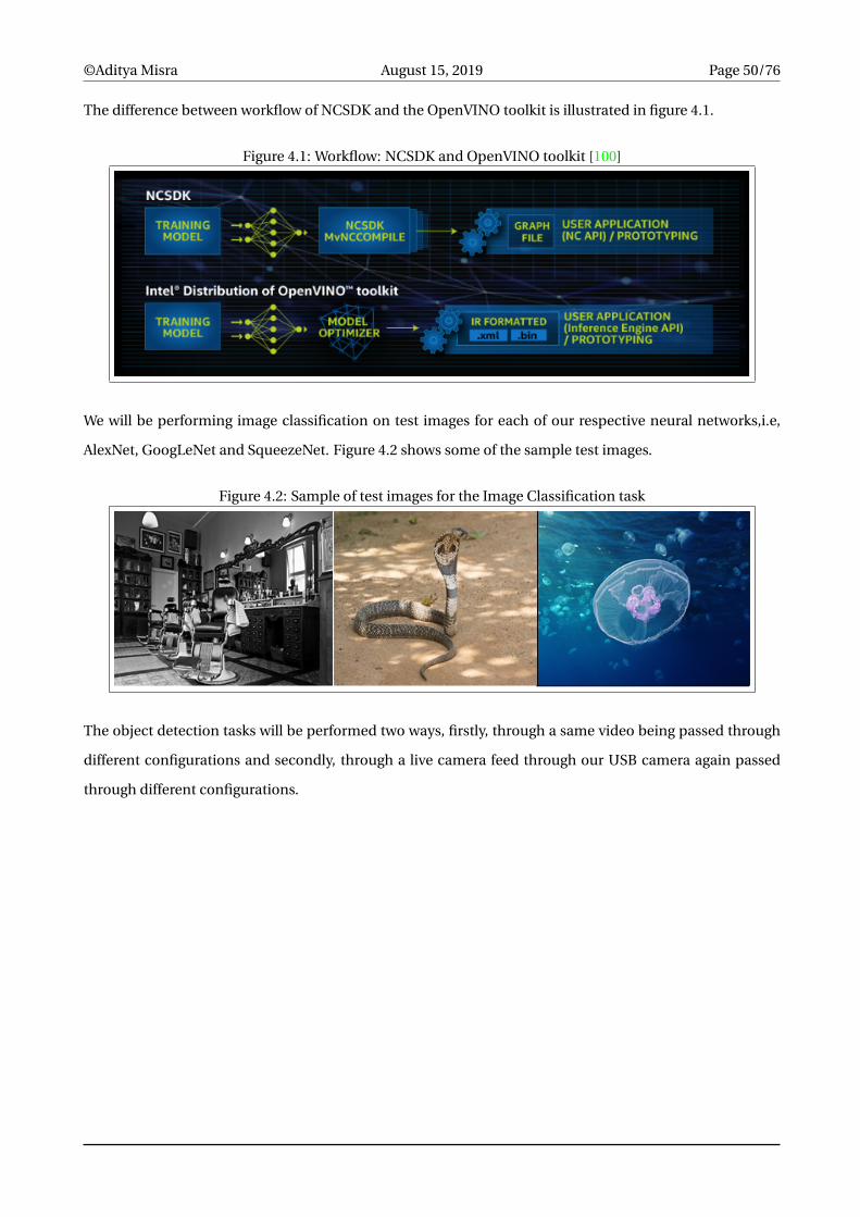
©Aditya Misra August 15, 2019 Page 50/76
The difference between workflow of NCSDK and the OpenVINO toolkit is illustrated in figure 4.1.
Figure 4.1: Workflow: NCSDK and OpenVINO toolkit [100]
We will be performing image classification on test images for each of our respective neural networks,i.e,
AlexNet, GoogLeNet and SqueezeNet. Figure 4.2 shows some of the sample test images.
Figure 4.2: Sample of test images for the Image Classification task
The object detection tasks will be performed two ways, firstly, through a same video being passed through
different configurations and secondly, through a live camera feed through our USB camera again passed
through different configurations.
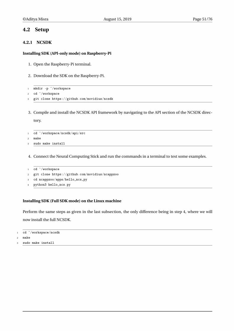
©Aditya Misra August 15, 2019 Page 51/76
4.2 Setup
4.2.1 NCSDK
Installing SDK (API-only mode) on Raspberry-Pi
1. Open the Raspberry-Pi terminal.
2. Download the SDK on the Raspberry-Pi.
1 mkdir -p ~/workspace2 cd ~/workspace3 git clone https://github.com/movidius/ncsdk
3. Compile and install the NCSDK API framework by navigating to the API section of the NCSDK direc-
tory.
1 cd ~/workspace/ncsdk/api/src2 make3 sudo make install
4. Connect the Neural Computing Stick and run the commands in a terminal to test some examples.
1 cd ~/workspace2 git clone https://github.com/movidius/ncappzoo3 cd ncappzoo/apps/hello_ncs_py4 python3 hello_ncs.py
Installing SDK (Full SDK mode) on the Linux machine
Perform the same steps as given in the last subsection, the only difference being in step 4, where we will
now install the full NCSDK.
1 cd ~/workspace/ncsdk2 make3 sudo make install

©Aditya Misra August 15, 2019 Page 52/76
4.2.2 OpenVINO
OpenVINO setup on Raspberry-Pi
1. Install OpenVINO + OpenCV dependencies on the Raspberry Pi.
2. Download and extract the OpenVINO toolkit on the Raspberry Pi [111].
3. Configure OpenVINO on the Raspberry Pi.
4. Configure USB rules and install dependencies for the Intel Movidius NCS and OpenVINO on the Rasp-
berry Pi.
5. Create a virtual environment for OpenVINO implementation, install the necessary packages and test
the OpenVINO install on your Raspberry Pi to get a successful output.
4.2.3 Hardware Setup
The final hardware setup with Intel Neural Computing Stick attached to the Raspberry-Pi is as shown in
figure 4.3.
Figure 4.3: Hardware Setup showing Intel NCS attached to the Raspberry-Pi
©Aditya Misra August 15, 2019 Page 53/76
4.3 Configurations
4.3.1 Configuration 1: Only Raspberry-Pi CPU
Image Classification
1. On the Linux machine, choose the respective CNN architectures and define their parameters in a
configuration file with extension .prototxt .
2. Generate a .caffemodel trained model to make prediction on the unseen data
3. Copy the generated respective Caffe models and their associated prototxt files to the Raspberry Pi.
4. Install the OpenCV library on the Raspberry Pi (minimum version 3.3).
5. Write a python script where the OpenCV DNN module is used for performing Image Classification
using the generated Caffe models.
6. Execute the python script in the Raspberry Pi terminal providing the path to the Caffe models, their
protxt files and class labels file and the test image to generate a successful inference.
Object Detection
1. On the Linux machine, choose the respective CNN architecture and define its parameters in a config-
uration file with extension .prototxt .
2. Generate a .caffemodel trained model to make prediction on the unseen data.
3. Copy the generated respective Caffe models and their associated prototxt files to the Raspberry Pi.
4. Install the OpenCV library on the Raspberry Pi (minimum version 3.3).
5. Write a python script where the OpenCV DNN module is used for performing Real time Object Detec-
tion using the generated Caffe models.
6. Execute the python script in the Raspberry Pi terminal providing the path to the Caffe models, their
protxt files and class labels file and the test image to generate a successful inference.
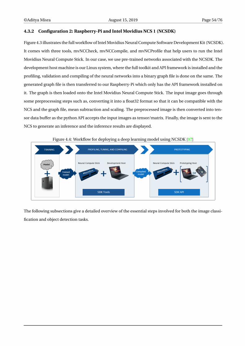
©Aditya Misra August 15, 2019 Page 54/76
4.3.2 Configuration 2: Raspberry-Pi and Intel Movidius NCS 1 (NCSDK)
Figure 4.3 illustrates the full workflow of Intel Movidius Neural Compute Software Development Kit (NCSDK).
It comes with three tools, mvNCCheck, mvNCCompile, and mvNCProfile that help users to run the Intel
Movidius Neural Compute Stick. In our case, we use pre-trained networks associated with the NCSDK. The
development host machine is our Linux system, where the full toolkit and API framework is installed and the
profiling, validation and compiling of the neural networks into a binary graph file is done on the same. The
generated graph file is then transferred to our Raspberry-Pi which only has the API framework installed on
it. The graph is then loaded onto the Intel Movidius Neural Compute Stick. The input image goes through
some preprocessing steps such as, converting it into a float32 format so that it can be compatible with the
NCS and the graph file, mean subtraction and scaling. The preprocessed image is then converted into ten-
sor data buffer as the python API accepts the input images as tensor/matrix. Finally, the image is sent to the
NCS to generate an inference and the inference results are displayed.
Figure 4.4: Workflow for deploying a deep learning model using NCSDK [97]
The following subsections give a detailed overview of the essential steps involved for both the image classi-
fication and object detection tasks.

©Aditya Misra August 15, 2019 Page 55/76
Image Classification
1. On the Linux machine with the full SDK, use the mvNCCompile tool of the SDK to generate graph files
through conversion of the respective Caffe models.
2. Copy the generated graphs to the Raspberry Pi.
3. Next we will perform some steps by writing a python script for performing Image Classification using
the respective neural networks (AlexNet, GoogLeNEt and SqueezeNet) and generating a successful
inference:
• Import the necessary packages.
• Import class labels and image.
• List all connected NCS devices.
1 devices = mvnc.EnumerateDevices()
• Select and open the NCS device.
1 device = mvnc.Device(devices[0])2 device.OpenDevice()
• Load the graph file into Raspberry Pi memory.
1 with open(args["graph"], mode="rb") as f:2 graph_in_memory = f.read()
• Load the graph on the NCS.
1 graph = device.AllocateGraph(graph_in_memory)
• Classify the image with the NCS and the API.
1 # Call graph.LoadTensor to make a prediction2 graph.LoadTensor(image.astype(np.float16), "user object")3 # Call graph.GetResult to grab the resulting predictions.4 (preds, userobj) = graph.GetResult()
• Close the device and deallocate the graph.
1 graph.DeallocateGraph()2 device.CloseDevice()
• Display the output image, predicted label and the associated probability to the console.
4. Execute the Python script in the Raspberry Pi terminal providing the path to the generated graph, test
image and class labels file to generate a successful inference for each neural network.

©Aditya Misra August 15, 2019 Page 56/76
Object Detection
1. On the Linux machine with the full SDK, use the mvNCCompile tool of the SDK to generate a graph
file through conversion of the respective Caffe model.
2. Copy the generated graph to the Raspberry Pi.
3. Next we will perform some steps by writing a python script for performing real time object detection
using MobileNet-SSD and generating a successful inference:
• Import the necessary packages.
• Define a function to preprocess the image to scale it and convert it to float16 format.
• Define a predict function that will send the preprocessed image to the NCS and output the net-
work predictions.
1 graph.LoadTensor(image, None)
• Connect the NCS and load the graph file on it.
1 devices = mvnc.EnumerateDevices()2 device = mvnc.Device(devices[0])3 device.OpenDevice()4 with open(args["graph"], mode="rb") as f:5 graph_in_memory = f.read()6 graph = device.AllocateGraph(graph_in_memory)
• Start the video stream and FPS counter.
• Use the NCS to acquire predictions.
1 frame = vs.read()2 predictions = predict(frame, graph)
• Close the device and deallocate the graph.
1 graph.DeallocateGraph()2 device.CloseDevice()
• Close the device and deallocate the graph.
1 graph.DeallocateGraph()2 device.CloseDevice()
4. Execute the Python script in the Raspberry Pi terminal, providing the path to the generated graph, to
generate a successful inference.
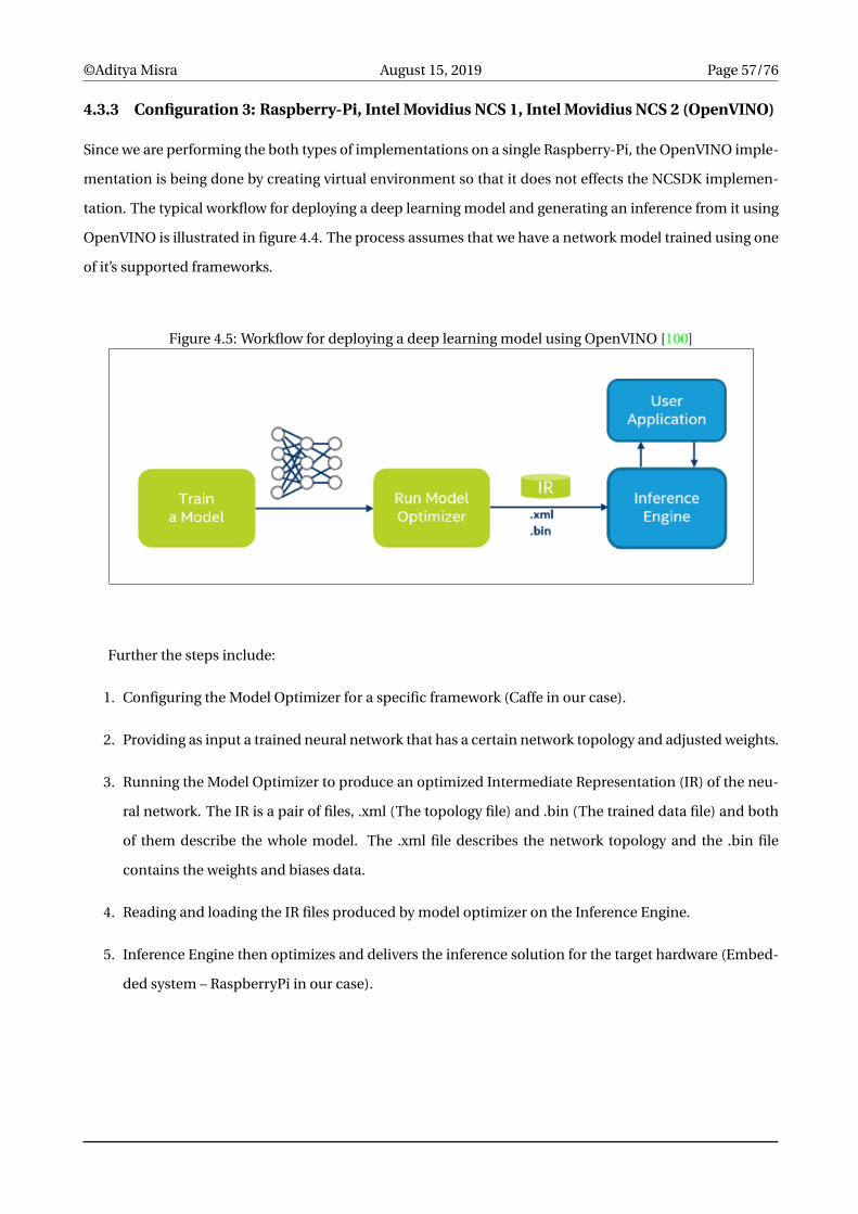
©Aditya Misra August 15, 2019 Page 57/76
4.3.3 Configuration 3: Raspberry-Pi, Intel Movidius NCS 1, Intel Movidius NCS 2 (OpenVINO)
Since we are performing the both types of implementations on a single Raspberry-Pi, the OpenVINO imple-
mentation is being done by creating virtual environment so that it does not effects the NCSDK implemen-
tation. The typical workflow for deploying a deep learning model and generating an inference from it using
OpenVINO is illustrated in figure 4.4. The process assumes that we have a network model trained using one
of it’s supported frameworks.
Figure 4.5: Workflow for deploying a deep learning model using OpenVINO [100]
Further the steps include:
1. Configuring the Model Optimizer for a specific framework (Caffe in our case).
2. Providing as input a trained neural network that has a certain network topology and adjusted weights.
3. Running the Model Optimizer to produce an optimized Intermediate Representation (IR) of the neu-
ral network. The IR is a pair of files, .xml (The topology file) and .bin (The trained data file) and both
of them describe the whole model. The .xml file describes the network topology and the .bin file
contains the weights and biases data.
4. Reading and loading the IR files produced by model optimizer on the Inference Engine.
5. Inference Engine then optimizes and delivers the inference solution for the target hardware (Embed-
ded system – RaspberryPi in our case).

©Aditya Misra August 15, 2019 Page 58/76
Object Detection
1. On the Linux machine, choose the respective CNN architecture (MobileNet-SSD) and define its pa-
rameters in a configuration file with extension .prototxt.
2. Generate a .caffemodel trained model to make prediction on the unseen data.
3. Copy the generated Caffe model and its associated prototxt file to the Raspberry Pi.
4. Perform the following steps by writing a python script for performing Real Time Object Detection
using MobileNet-SSD and generating a successful inference:
• Import the necessary packages.
• Load the model from the disk.
• Specify the target device as the Myriad processor on the Intel Neural Computing Sticks 1 and 2.
1 setPreferableTarget(cv2.dnn.DNN_TARGET_MYRIAD)
• Start the video stream and FPS counter.
• Loop over the frames from the video stream, grab the frame dimensions, convert it to a blob, and
pass the blob through the neural network to obtain the detections and predictions.
5. Execute the python script in the Raspberry Pi terminal, providing the path to the Caffe model and its
protxt file to generate a successful inference.
©Aditya Misra August 15, 2019 Page 59/76
Chapter 5
Evaluation
This chapter presents the evaluation results of this dissertation. As a part of the deep learning experiments,
we perform Image Classification and Object Detection tasks using multiple configurations and collect the
results. We evaluate the performance metrics and compare the performance against a set baseline to verify
the effectiveness of the deep learning accelerators. The videos results regarding the Object Detection can
be found on the attached CD.
5.1 Evaluation Parameters
The evaluation parameters are the following:
• Inference time (for Image Classification tasks)
• Frames per second (for Object Detection tasks)
We consider the performance of the Raspberry Pi CPU for Image Classification and Object Detection tasks
as a baseline for benchmarking the other results. The performance of the Raspberry Pi with respect to the
Deep Learning tasks with and without the Deep learning accelerators is compared as a part of the research.
When using the Raspberry Pi for deep learning we have two major pitfalls working against us:
• Restricted memory
• Limited processor speed
Therefore, it is expected that the larger, deeper neural networks would not give a preferable performance
and instead, smaller networks such as SqueezeNet will stand out in terms of performance. In the further
subsections the results of the neural networks and their associated measured performance will verify the
same.

©Aditya Misra August 15, 2019 Page 60/76
5.2 Experiments
5.2.1 Image Classification
We evaluate our image classification task on a set of 2000 test images, some of which showing the resulting
classification confidence percentage can be seen in the figure 5.1. Configuration 1 (Only RaspberryPi CPU)
and Configuration 2 (RaspberryPi and Movidius NCS 1 (NCSDK)) are used for performing the image classi-
fication task.
Figure 5.1: Some sample test results showing classification confidence percentage
We have taken a mix of color and non-color images, but due to our process of using the OpenCV’s DNN
module to convert the image into a Binary Large Object (BLOB), the color and non-color images eventually
are treated the same.
Furthermore, to keep the resolution of the input images same, we are pre-processing (normalizing) the im-
age to dimensions of 227 x 227, which are the image dimensions SqueezeNet was trained on (similarly, 227
x 227 for AlexNet and 224 x 224 for GoogLeNet to be consistent with the prototxt definitions) and scaling the
image further using mean subtraction. In case of using the Movidius NCS, a further action of converting the
image array data to float32 format is done, since it is a requirement for the NCS.
In the case of Configuration 1, we pass (forward) the BLOB through the respective neural network to gener-
ate classification predictions. In the case of Configuration 2, we classify the image with the NCS and its API
using a two-step process, loading our prior generated graph object as tensor matrix to generate a prediction
and then saving the resulting predictions.
Finally, in both the configurations, we derive the highest predicted class label and corresponding probability
on the image, sort and display the top five results.
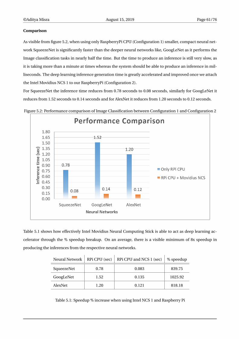
©Aditya Misra August 15, 2019 Page 61/76
Comparison
As visible from figure 5.2, when using only RaspberryPi CPU (Configuration 1) smaller, compact neural net-
work SqueezeNet is significantly faster than the deeper neural networks like, GoogLeNet as it performs the
Image classification tasks in nearly half the time. But the time to produce an inference is still very slow, as
it is taking more than a minute at times whereas the system should be able to produce an inference in mil-
liseconds. The deep learning inference generation time is greatly accelerated and improved once we attach
the Intel Movidius NCS 1 to our RaspberryPi (Configuration 2).
For SqueezeNet the inference time reduces from 0.78 seconds to 0.08 seconds, similarly for GoogLeNet it
reduces from 1.52 seconds to 0.14 seconds and for AlexNet it reduces from 1.20 seconds to 0.12 seconds.
Figure 5.2: Performance comparison of Image Classification between Configuration 1 and Configuration 2
Table 5.1 shows how effectively Intel Movidius Neural Computing Stick is able to act as deep learning ac-
celerator through the % speedup breakup. On an average, there is a visible minimum of 8x speedup in
producing the inferences from the respective neural networks.
Neural Network RPi CPU (sec) RPi CPU and NCS 1 (sec) % speedup
SqueezeNet 0.78 0.083 839.75
GoogLeNet 1.52 0.135 1025.92
AlexNet 1.20 0.121 818.18
Table 5.1: Speedup % increase when using Intel NCS 1 and Raspberry Pi

©Aditya Misra August 15, 2019 Page 62/76
5.2.2 Object Detection
Figure 5.3 shows sample results when performing Object Detection. The Object Detection has been per-
formed in all our 3 configurations, Configuration 1 (Only RaspberryPi CPU), Configuration 2 (RaspberryPi
and Movidius NCS 1 (NCSDK)) and Configuration 3 (RaspberryPi, Movidius NCS 1, Movidius NCS 2 (Open-
VINO)).
The object detection has been performed in two ways, firstly by using a random YouTube video as an input
and then recognising objects in it, and secondly, through the use of a USB camera, taking in a live stream of
video as input and then identifying objects in it.
As can be seen from the figure 5.3, the deep learning network MobileNetSSD is correctly identifying objects
like person and TV monitor in the left photo when using a live USB camera feed and it also successfully
identifies objects like car and person in the right photo, which is a frame of a YouTube video given as the
input.
Since, the performance metric for Object Detection is Frames per second (FPS), the clear difference is seen
in the videos of the individual configurations provided in the CD.
For current comparison sake, we are taking a random YouTube video as our input and processing it frame by
frame to detect the objects in it. This is the case because we are calculating the FPS over multiple instances
over a same set of frames, taking the average and verifying if it is in a reasonable deviation range for a set
amount of video run-time. A live USB camera feed would not be an ideal case because the video setting will
always be dynamic, with objects being added or subtracted from a frame each time.
Figure 5.3: Sample result showing Object Detection in video frames

©Aditya Misra August 15, 2019 Page 63/76
Comparison
Figure 5.4 shows the average FPS comparison respective to each configuration. As can it can be seen, the
average FPS (0.59) is very poor for a standalone Raspberry Pi CPU (Configuration 1), unsuitable for Ob-
ject Detection. The slow frame rate and lagging frames can be seen in the video associated with the same
(provided in the CD). The average FPS greatly improves in Configuration 2, upon the application of Intel
Movidius Neural Computing stick to the RaspberryPi. The average FPS of Configuration 2 (3.80) is nearly 6x
times of Configuration 1. In Configuration 3, when RaspberryPi, Intel NCS 1 and OpenVINO are combined
the FPS further rises by 1.1x times (4.20) of Configuration 2 and when when RaspberryPi, Intel NCS 2 and
OpenVINO are combined the FPS further rises by 1.2x (5.11) in the same configuration.
Figure 5.4: Performance comparison of Object Detection among Configuration 1, 2 and 3
Table 5.2 shows the further breakup in terms of average time per frame. Starting from our base Configura-
tion 1 and moving to Configuration 3, the average process time per frame reduces from 1.6 seconds to 0.19
seconds, which is nearly 8.5x speedup from the baseline.
Configurations MobileNetSSD FPS average time per frame (sec)
RPi CPU 0.59 1.6
RPi CPU and NCS 1 (NCSDK) 3.8 0.27
RPi CPU and NCS 1 (OpenVINO) 4.20 0.23
RPi CPU and NCS 2 (OpenVINO) 5.11 0.19
Table 5.2: FPS benchmark comparison
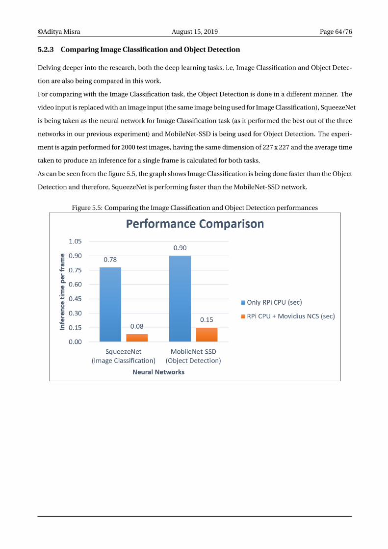
©Aditya Misra August 15, 2019 Page 64/76
5.2.3 Comparing Image Classification and Object Detection
Delving deeper into the research, both the deep learning tasks, i.e, Image Classification and Object Detec-
tion are also being compared in this work.
For comparing with the Image Classification task, the Object Detection is done in a different manner. The
video input is replaced with an image input (the same image being used for Image Classification), SqueezeNet
is being taken as the neural network for Image Classification task (as it performed the best out of the three
networks in our previous experiment) and MobileNet-SSD is being used for Object Detection. The experi-
ment is again performed for 2000 test images, having the same dimension of 227 x 227 and the average time
taken to produce an inference for a single frame is calculated for both tasks.
As can be seen from the figure 5.5, the graph shows Image Classification is being done faster than the Object
Detection and therefore, SqueezeNet is performing faster than the MobileNet-SSD network.
Figure 5.5: Comparing the Image Classification and Object Detection performances
©Aditya Misra August 15, 2019 Page 65/76
Chapter 6
Conclusion
In this chapter, we discuss our work, identify how it can be useful for future research, present some limita-
tions of our work and finally, we detail possible future work.
6.1 Research Contribution
A novel design concept and its implementation was presented in this dissertation project. It shows how
effective the AI accelerators(Intel Neural Computing Sticks) are and how they can assist in optimizing and
accelerating the state of the art Deep Learning concepts in low power and compact embedded system de-
vices (Raspberry Pi in this case).
Three different configurations are implemented in this dissertation, Configuration 1 (Only Raspberry-Pi
CPU), Configuration 2 (Raspberry-Pi and Intel NCS 1 (NCSDK)) and Configuration 3 (Raspberry-Pi, Intel
NCS 1 and Intel NCS 2 (OpenVINO)). Configuration 1’s results were used to benchmark the performance of
other two configurations.
6.2 Discussion
The Image Classification task was performed with Configuration 1 and 2, with Configuration 2 consisting of
Intel NCS 1 giving the best results. Configuration 2 greatly accelerated the deep learning task and performed
the same utp 9-11X times faster than Configuration 1. Further the results depict that compact and computa-
tionally efficient neural networks such as SqueezeNet and MobileNetSSD perform significantly better than
our other deeper neural networks such as, GoogLeNet and AlexNet, which is extremely important since we
are applying deep learning to the resource constrained Raspberry Pi.
©Aditya Misra August 15, 2019 Page 66/76
The Object Detection task was performed using Configuration 1, 2 and 3, with Configuration 3 consist-
ing of Intel NCS 2 and OpenVINO giving the best results. Configuration 1 gave an FPS of only 0.59 which
was very poor for the Object Detection, Configuration 2 and 3 greatly accelerated the FPS nearly 8.5X times
up to the range of 5-6 FPS, which can be considered suitable for Object Detection.
The results depict that the Raspberry Pi can be used as an embedded deep learning device and is well capa-
ble of performing complex tasks like Object Detection and Image Classification when combined with an AI
accelerator. This project depicts the ability of a low power and low cost inference model runner and shows
how the deep learning applications can be transitioned from the desktop PCs to current edge devices. With
growing research into low powered embedded intelligence devices, this work shows the capability of the
deep learning accelerators and their potential for application in other Deep Learning research areas for the
future.
6.3 Limitations
1. The Raspberry Pi lacks a USB 3.0. It has a USB 2.0, which has a lower clock speed and is slower than a
USB 3.0 bus. It reduces the speed with which the data can flow into the Intel Neural computing stick
from the host Raspberry Pi system.
2. Intel Movidius Neural Compute Stick has a number of limitations currently, as its current SDK does
not support many operations.
3. Only a limited number of Convolutional Neural Networks are currently available and associated with
the Movidius toolkit. It should be enhanced to include many of the successful CNNs for more robust
performance results.
4. Presently, Movidius does not support training of the deep learning convolutional neural networks.
This limits all applications related to on-line learning of a deep learning network.

©Aditya Misra August 15, 2019 Page 67/76
6.4 Future Work
1. The effectiveness of using multiple Intel Neural Computing Sticks in parallel can be explored.
2. The neural networks can be further fine-tuned to increase the accuracy of the results.
3. Caffe framework is used in this dissertation as it was the one more easily available configurable and
applicable for all the combinations. the same combinations can be applied through the TensorFlow
framework to verify if there is a considerable difference in the results.
4. MobileNetSSD is used for object detection. However, TinyYOLO is also available under the Movid-
ius software toolkit. The TinyYOLO implementation can be performed and can be compared to the
MobileNetSSD implementation.
5. Other state of the art AI accelerators, such as an Nvidia Jetson Nano can be explored.
©Aditya Misra August 15, 2019 Page 68/76
Bibliography
[1] Dana H. Ballard; Christopher M. Brown (1982). Computer Vision. Prentice Hall. ISBN 978-0-13-165316-
0.
[2] Huang, T. (1996-11-19). Vandoni, Carlo, E (ed.). Computer Vision : Evolution And Promise (PDF). 19th
CERN School of Computing. Geneva: CERN. pp. 21–25. doi:10.5170/CERN-1996-008.21. ISBN 978-
9290830955..
[3] Milan Sonka; Vaclav Hlavac; Roger Boyle (2008). Image Processing, Analysis, and Machine Vision.
Thomson. ISBN 978-0-495-08252-1.
[4] Reinhard Klette (2014). Concise Computer Vision. Springer. ISBN 978-1-4471-6320-6.
[5] Linda G. Shapiro; George C. Stockman (2001). Computer Vision. Prentice Hall. ISBN 978-0-13-030796-5.
[6] Tim Morris (2004). Computer Vision and Image Processing. Palgrave Macmillan. ISBN 978-0-333-99451-
1.
[7] Bernd Jähne; Horst Haußecker (2000). Computer Vision and Applications, A Guide for Students and
Practitioners. Academic Press. ISBN 978-0-13-085198-7.
[8] David A. Forsyth; Jean Ponce (2003). Computer Vision, A Modern Approach. Prentice Hall. ISBN 978-0-
13-085198-7.
[9] Hubel, D.H. and Wiesel, T.N., 1959. Receptive fields of single neurones in the cat’s striate cortex. The
Journal of physiology, 148(3), pp.574-591.
[10] Roberts, L.G., 1963. Machine perception of three-dimensional solids (Doctoral dissertation, Mas-
sachusetts Institute of Technology).
[11] Marr, D., 1982. Vision: A computational investigation into the human representation and processing
of visual information.
[12] Fukushima, K.; Miyake, S.; Ito, T. (1983). "Neocognitron: a neural network model for a mechanism of
visual pattern recognition". IEEE Transactions on Systems, Man, and Cybernetics. SMC-13 (3): 826–834.

©Aditya Misra August 15, 2019 Page 69/76
[13] LeCun, Y. and Bengio, Y., 1995. Convolutional networks for images, speech, and time series. The hand-
book of brain theory and neural networks, 3361(10), p.1995.
[14] Lowe, D.G., 1999, September. Object recognition from local scale-invariant features. In iccv (Vol. 99,
No. 2, pp. 1150-1157).
[15] Viola, P. and Jones, M., 2001. Rapid object detection using a boosted cascade of simple features. CVPR
(1), 1, pp.511-518
[16] Felzenszwalb, P.F., McAllester, D.A. and Ramanan, D., 2008, June. A discriminatively trained, multiscale,
deformable part model. In Cvpr (Vol. 2, No. 6, p. 7).
[17] Guyon, I., Gunn, S., Nikravesh, M. and Zadeh, L.A. eds., 2008. Feature extraction: foundations and
applications (Vol. 207). Springer
[18] Ke, Y. and Sukthankar, R., 2004. PCA-SIFT: A more distinctive representation for local image descrip-
tors. CVPR (2), 4, pp.506-513.
[19] Bay, H., Tuytelaars, T. and Van Gool, L., 2006, May. Surf: Speeded up robust features. In European
conference on computer vision (pp. 404-417). Springer, Berlin, Heidelberg.
[20] Dalal, N. and Triggs, B., 2005, June. Histograms of oriented gradients for human detection. In interna-
tional Conference on computer vision Pattern Recognition (CVPR’05) (Vol. 1, pp. 886-893). IEEE Com-
puter Society.
[21] Rublee, E., Rabaud, V., Konolige, K. and Bradski, G.R., 2011, November. ORB: An efficient alternative to
SIFT or SURF. In ICCV (Vol. 11, No. 1, p. 2).
[22] Bengio, Y.; Courville, A.; Vincent, P. (2013). "Representation Learning: A Review and New Perspectives".
IEEE Transactions on Pattern Analysis and Machine Intelligence. 35 (8): 1798–1828. arXiv:1206.5538.
doi:10.1109
[23] Schmidhuber, J. (2015). "Deep Learning in Neural Networks: An Overview". Neural Networks. 61:
85–117. arXiv:1404.7828. doi:10.1016/j.neunet.2014.09.003.
[24] Bengio, Yoshua; LeCun, Yann; Hinton, Geoffrey (2015). "Deep Learning". Nature. 521 (7553): 436–444.
Bibcode:2015Natur.521..436L. doi:10.1038..
[25] Bengio, Yoshua (2009). "Learning Deep Architectures for AI" (PDF). Foundations and Trends in Ma-
chine Learning. 2 (1): 1–127. CiteSeerX 10.1.1.701.9550. doi:10.1561/2200000006
[26] Smith, Stephen W (1997). "13.Convolution". The Scientist and Engineer’s Guide to Digital Signal Pro-
cessing (1 ed.). California Technical Publishing. ISBN 0966017633
©Aditya Misra August 15, 2019 Page 70/76
[27] Alex Krizhevsky, Ilya Sutskever, Geoffrey E. Hinton, ”ImageNet classification withdeep convolutional
neural networks”, NIPS’12 Proceedings of the 25th InternationalConference on Neural Information Pro-
cessing Systems - Volume 1 Pages 1097-1105
[28] Hopfield, J. J. (1982). "Neural networks and physical systems with emergent collective computational
abilities". Proc. Natl. Acad. Sci. U.S.A. 79 (8): 2554–2558. doi:10.1073/pnas.79.8.2554
[29] McCulloch, Warren; Walter Pitts (1943). "A Logical Calculus of Ideas Immanent in Nervous Activity".
Bulletin of Mathematical Biophysics. 5 (4): 115–133. doi:10.1007/BF02478259.
[30] Rosenblatt, F. (1958). "The Perceptron: A Probalistic Model For Information Storage And Organization
In The Brain". Psychological Review. 65 (6): 386–408. CiteSeerX 10.1.1.588.3775
[31] Werbos, P.J. (1975). Beyond Regression: New Tools for Prediction and Analysis in the Behavioral Sci-
ences.
[32] LeCun, Y., Bottou, L., Bengio, Y. and Haffner, P., 1998. Gradient-based learning applied to document
recognition. Proceedings of the IEEE, 86(11), pp.2278-2324.
[33] Fei-Fei Li, Andrej Karpathy. CS231n: Convolutional Neural Networks for Visual Recognition, Spring
2019.
[34] Shyamal Patel, Johanna Pingel, Introduction to Deep Learning: What Are Convolutional Neural Net-
works, Mathworks UK.
[35] Szegedy, C., Liu, W., Jia, Y., Sermanet, P., Reed, S., Anguelov, D., Erhan, D., Vanhoucke, V. and Rabi-
novich, A., 2015. Going deeper with convolutions. In Proceedings of the IEEE conference on computer
vision and pattern recognition (pp. 1-9).
[36] Ioffe, S. and Szegedy, C., 2015. Batch normalization: Accelerating deep network training by reducing
internal covariate shift. arXiv preprint arXiv:1502.03167.
[37] Szegedy, C., Vanhoucke, V., Ioffe, S., Shlens, J. and Wojna, Z., 2016. Rethinking the inception archi-
tecture for computer vision. In Proceedings of the IEEE conference on computer vision and pattern
recognition (pp. 2818-2826).
[38] Szegedy, C., Ioffe, S., Vanhoucke, V. and Alemi, A.A., 2017, February. Inception-v4, inception-resnet
and the impact of residual connections on learning. In Thirty-First AAAI Conference on Artificial Intel-
ligence.
[39] He, K., Zhang, X., Ren, S. and Sun, J., 2016. Deep residual learning for image recognition. In Proceedings
of the IEEE conference on computer vision and pattern recognition (pp. 770-778).
©Aditya Misra August 15, 2019 Page 71/76
[40] He, K., Zhang, X., Ren, S. and Sun, J., 2016, October. Identity mappings in deep residual networks. In
European conference on computer vision (pp. 630-645). Springer, Cham.
[41] Zagoruyko, S. and Komodakis, N., 2016. Wide residual networks. arXiv preprint arXiv:1605.07146.
[42] Iandola, F.N., Han, S., Moskewicz, M.W., Ashraf, K., Dally, W.J. and Keutzer, K., 2016. SqueezeNet:
AlexNet-level accuracy with 50x fewer parameters and< 0.5 MB model size. arXiv preprint
arXiv:1602.07360.
[43] Howard, A.G., Zhu, M., Chen, B., Kalenichenko, D., Wang, W., Weyand, T., Andreetto, M. and Adam, H.,
2017. Mobilenets: Efficient convolutional neural networks for mobile vision applications. arXiv preprint
arXiv:1704.04861.
[44] Girshick, R., Donahue, J., Darrell, T. and Malik, J., 2014. Rich feature hierarchies for accurate object
detection and semantic segmentation. In Proceedings of the IEEE conference on computer vision and
pattern recognition (pp. 580-587).
[45] Uijlings, J.R., Van De Sande, K.E., Gevers, T. and Smeulders, A.W., 2013. Selective search for object
recognition. International journal of computer vision, 104(2), pp.154-171.
[46] Girshick, R., 2015. Fast r-cnn. In Proceedings of the IEEE international conference on computer vision
(pp. 1440-1448).
[47] Ren, S., He, K., Girshick, R. and Sun, J., 2015. Faster r-cnn: Towards real-time object detection with
region proposal networks. In Advances in neural information processing systems (pp. 91-99).
[48] Redmon, J., Divvala, S., Girshick, R. and Farhadi, A., 2016. You only look once: Unified, real-time object
detection. In Proceedings of the IEEE conference on computer vision and pattern recognition (pp. 779-
788).
[49] Liu, W., Anguelov, D., Erhan, D., Szegedy, C., Reed, S., Fu, C.Y. and Berg, A.C., 2016, October. Ssd: Single
shot multibox detector. In European conference on computer vision (pp. 21-37). Springer, Cham.
[50] Dai, J., Li, Y., He, K. and Sun, J., 2016. R-fcn: Object detection via region-based fully convolutional
networks. In Advances in neural information processing systems (pp. 379-387).
[51] Embedded Vision alliance What is Embedded Vision. https://www.embedded-vision.com/
what-is-embedded-vision. Accessed 15 July 2019.
[52] Kisacanin, B., Bhattacharyya, S.S. and Chai, S. eds., 2008. Embedded computer vision. Springer Science
Business Media.

©Aditya Misra August 15, 2019 Page 72/76
[53] Kisacanin, B. and Gelautz, M. eds., 2014. Advances in embedded computer vision. Springer Interna-
tional Publishing.
[54] Stewart, R.J., Bhowmik, D., Wallace, A.M., Michaelson, G.: Profile Guided Dataflow Transformation for
FPGAs and CPUs. Signal Processing Systems 87(1), 3–20 (2017)
[55] Bhowmik, D., Garcia, P., Wallace, A., Stewart, R., Michaelson, G.: Power efficient dataflow design for a
heterogeneous smart camera architecture. In: Conference on Design and Architectures for Signal and
Image Processing (DASIP 2017) (August 2017)
[56] Bhowmik, D. and Appiah, K., 2018. Embedded vision systems: A review of the literature.
[57] Upton, E. and Halfacree, G., 2014. Raspberry Pi user guide. John Wiley Sons.
[58] Banzi, M. and Shiloh, M., 2014. Getting started with Arduino: the open source electronics prototyping
platform. Maker Media, Inc.
[59] Su, M., Tan, J., Lin, C.Y., Ye, J., Wang, C.H. and Hung, C.L., 2015, August. Constructing a Mobility and
Acceleration Computing Platform with NVIDIA Jetson TK1. In 2015 IEEE 17th International Conference
on High Performance Computing and Communications, 2015 IEEE 7th International Symposium on
Cyberspace Safety and Security, and 2015 IEEE 12th International Conference on Embedded Software
and Systems (pp. 1854-1858). IEEE.
[60] Otterness, N., Yang, M., Rust, S., Park, E., Anderson, J.H., Smith, F.D., Berg, A. and Wang, S., 2017, April.
An evaluation of the NVIDIA TX1 for supporting real-time computer-vision workloads. In 2017 IEEE
Real-Time and Embedded Technology and Applications Symposium (RTAS) (pp. 353-364). IEEE.
[61] Sahani, M., Mohanty, M.N.: Realization of different algorithms using raspberry pi for realtime image
processing application. In: Intelligent Computing, Communication and Devices,pp. 473–479. Springer
(2015)
[62] Buechley, L., Eisenberg, M., Catchen, J. and Crockett, A., 2008, April. The LilyPad Arduino: using com-
putational textiles to investigate engagement, aesthetics, and diversity in computer science education.
In Proceedings of the SIGCHI conference on Human factors in computing systems (pp. 423-432). ACM.
[63] Wang, G., Xiong, Y., Yun, J., Cavallaro, J.R.: Accelerating computer vision algorithms using opencl
framework on the mobile gpu - a case study. In: 2013 IEEE International Conference on Acoustics,
Speech and Signal Processing. pp. 2629–2633 (May 2013)
[64] Rister, B., Wang, G., Wu, M., Cavallaro, J.R.: A fast and efficient sift detector using the mobile GPU. In:
Proc. IEEE ICASSP. pp. 2674–2678 (2013)

©Aditya Misra August 15, 2019 Page 73/76
[65] Andargie, F.A., Rose, J., Austin, T., Bertacco, V.: Energy efficient object detection on the mobile gp-gpu.
In: 2017 IEEE AFRICON. pp. 945–950 (Sept 2017)
[66] Szegedy, C., Vanhoucke, V., Ioffe, S., Shlens, J., Wojna, Z.: Rethinking the inception architecture for
computer vision. In: The IEEE Conference on Computer Vision and Pattern Recognition (CVPR) (June
2016)
[67] Krizhevsky, A., Sutskever, I., Hinton, G.E.: Imagenet classification with deep convolutional neural net-
works. Commun. ACM 60(6), 84–90 (May 2017)
[68] Gokhale, V., Jin, J., Dundar, A., Martini, B., Culurciello, E.: A 240 g-ops/s mobile coprocessor for deep
neural networks. In: The IEEE Conference on Computer Vision and Pattern Recognition (CVPR) Work-
shops (June 2014)
[69] Sugiura, T., Yu, J., Takeuchi, Y., Imai, M.: A low-energy asip with flexible exponential golomb codec
for lossless data compression toward artificial vision systems. In: 2015 IEEE Biomedical Circuits and
Systems Conference (BioCAS). pp. 1–4 (Oct 2015)
[70] Su, J., Liu, J., Thomas, D.B., Cheung, P.Y.: Neural network based reinforcement learning acceleration
on fpga platforms. SIGARCH Comput. Archit. News 44(4), 68–73 (Jan 2017)
[71] Ho, S.M.H., Hung, C.H.D., Ng, H.C., Wang, M., So, H.K.H.: A parameterizable activation function gen-
erator for fpga-based neural network applications. In: IEEE 25th Annual International Symposium on
Field-Programmable Custom Computing Machines (FCCM) (2017)
[72] Bettoni, M., Urgese, G., Kobayashi, Y., Macii, E., Acquaviva, A.: A convolutional neural network fully
implemented on fpga for embedded platforms. In: 2017 New Generation of CAS (NGCAS). pp. 49–52
(Sept 2017)
[73] Colangelo, P., Luebbers, E., Huang, R., Margala, M., Nealis, K.: Application of convolutional neural
networks on intel; xeon; processor with integrated fpga. In: 2017 IEEE High Performance Extreme Com-
puting Conference (HPEC). pp. 1–7 (Sept 2017)
[74] Hamilton, Eric. "What is Edge Computing: The Network Edge Explained". cloudwards.net.
[75] Shi, W. and Dustdar, S., 2016. The promise of edge computing. Computer, 49(5), pp.78-81.
[76] Antonopoulos, N. and Gillam, L., 2010. Cloud computing. London: Springer.
[77] Shi, W., Cao, J., Zhang, Q., Li, Y. and Xu, L., 2016. Edge computing: Vision and challenges. IEEE Internet
of Things Journal, 3(5), pp.637-646.
©Aditya Misra August 15, 2019 Page 74/76
[78] Oh, C.S. and Yoon, J.M., 2019, February. Hardware Acceleration Technology for Deep-Learning in Au-
tonomous Vehicles. In 2019 IEEE International Conference on Big Data and Smart Computing (Big-
Comp) (pp. 1-3). IEEE.
[79] Chen, X., Zhang, H., Wu, C., Mao, S., Ji, Y. and Bennis, M., 2019, April. Performance optimization in
mobile-edge computing via deep reinforcement learning. In 2018 IEEE 88th Vehicular Technology Con-
ference (VTC-Fall) (pp. 1-6). IEEE.
[80] Custom On Device ML Models. https://ai.googleblog.com/2018/05/
custom-on-device-ml-models.html. Accessed 16 July 2019
[81] Feng, C., Sheng, T., Liang, Z., Zhuo, S., Zhang, X., Shen, L., Ardi, M., Berg, A.C., Chen, Y., Chen, B. and
Gauen, K., 2019. Low Power Inference for On-Device Visual Recognition with a Quantization-Friendly
Solution. arXiv preprint arXiv:1903.06791.
[82] Deep Learning is coming of age. https://www.intel.ai/deep-learning-is-coming-of-age/
#gs.hna7px Accessed 17 July 2019
[83] Du, L. and Du, Y., 2017. Hardware Accelerator Design for Machine Learning. In Machine Learning-
Advanced Techniques and Emerging Applications. IntechOpen.
[84] NVIDIA DGX2 WORLD’S MOST POWERFUL AI SYSTEM https://www.nvidia.com/en-us/
data-center/dgx-2/. Accessed 18 July 2019
[85] Markidis, S., Der Chien, S.W., Laure, E., Peng, I.B. and Vetter, J.S., 2018, May. Nvidia tensor core pro-
grammability, performance precision. In 2018 IEEE International Parallel and Distributed Processing
Symposium Workshops (IPDPSW) (pp. 522-531). IEEE.
[86] Rodriguez, A., Segal, E., Meiri, E., Fomenko, E., Kim, Y.J., Shen, H. and Ziv, B., 2018. Lower numerical
precision deep learning inference and training. Intel White Paper.
[87] Putnam A. The configurable cloud – accelerating hyperscale datacenter services with FPGA. In: IEEE
33rd International Conference on Data Engineering (ICDE); San Diego. 2017. p. 1587
[88] Microsoft Research - Microsoft unveils Project Brainwave for real-time AI https://www.microsoft.
com/en-us/research/blog/microsoft-unveils-project-brainwave/ Accessed 20 July 2019
[89] Chang AXM, Culurciello E. Hardware accelerators for recurrent neural networks on FPGA. In: IEEE
International Symposium on Circuits and Systems (ISCAS); MD, Baltimore. 2017. pp. 1-4
©Aditya Misra August 15, 2019 Page 75/76
[90] Sim J, Park J-S, Kim M, Bae D, Choi Y, Kim L-S. A 1.42TOPS/W deep convolution neural network recog-
nition processor for intelligent IoE systems. In: Proceeding of IEEE International Solid-State Circuits
Conference (ISSCC). Jan/Feb. 2016. pp. 264-265
[91] Bong K, Choi S, Kim C, Kang S, Kim Y, Yoo HJ. 14.6 A 0.62mW ultra-low-power convolutional-neural-
network face-recognition processor and a CIS integrated with always-on haar-like face detector. IEEE
International Solid-State Circuits Conference (ISSCC); San Francisco. 2017. pp. 248–249
[92] Desoli G et al. 4.1 A 2.9TOPS/W deep convolutional neural network SoC in FD-SOI 28nm for intelligent
embedded systems. In: IEEE International Solid-State Circuits Conference (ISSCC); San Francisco. 2017.
pp. 238–239
[93] Barry, B., Brick, C., Connor, F., Donohoe, D., Moloney, D., Richmond, R., O’Riordan, M. and Toma, V.,
2015. Always-on vision processing unit for mobile applications. IEEE Micro, 35(2), pp.56-66.
[94] Othman, N.A. and AYDIN, I., 2018, October. A New Deep Learning Application Based on Movidius NCS
for Embedded Object Detection and Recognition. In 2018 2nd International Symposium on Multidisci-
plinary Studies and Innovative Technologies (ISMSIT) (pp. 1-5). IEEE.
[95] Srinivasan, V., Meudt, S. and Schwenker, F., 2018, August. Deep Learning Algorithms for Emotion
Recognition on Low Power Single Board Computers. In IAPR Workshop on Multimodal Pattern Recog-
nition of Social Signals in Human-Computer Interaction (pp. 59-70). Springer, Cham.
[96] Cass, S., 2019. Taking AI to the edge: Google’s TPU now comes in a maker-friendly package. IEEE Spec-
trum, 56(5), pp.16-17.
[97] Intel® Neural Compute Stick https://software.intel.com/en-us/neural-compute-stick Ac-
cessed 21 July 2019
[98] Raspberry Pi 3 Model B+. https://www.raspberrypi.org/products/
raspberry-pi-3-model-b-plus/ Accessed 21 July 2019
[99] Downloads. https://www.raspberrypi.org/downloads/ Accessed 22 July 2019
[100] Deep Learning For Computer Vision. https://software.intel.com/en-us/openvino-toolkit/
deep-learning-cv Accessed 24 July 2019
[101] Chandan, G., Jain, A. and Jain, H., 2018, July. Real Time object detection and Tracking using Deep
Learning and openCV. In 2018 International Conference on Inventive Research in Computing Applica-
tions (ICIRCA) (pp. 1305-1308). IEEE.
©Aditya Misra August 15, 2019 Page 76/76
[102] Contains examples for the Movidius Neural Compute Stick. https://github.com/movidius/
ncappzoo Accessed 25 July 2019
[103] ImageNet. http://www.image-net.org/ Accessed 26 July 2019
[104] MS COCO. http://cocodataset.org/#home Accessed 28 July 2019
[105] Intel® Movidius™ Neural Compute Stick Blog. https://movidius.github.io/blog/mvNCCheck/
Accessed 30 July 2019
[106] Conventional computer vision coupled with deep learning makes AI better | Network
World.https://www.networkworld.com/article/3239146/internet-of-things/conventional-computer-
vision-coupled-with-deep-learning-makes-ai-better.html. Accessed 12 Sep 2018
[107] OpenCV 4.1.1. https://opencv.org/ Accessed 1 August 2019
[108] Zheng L, Yang Y, Tian Q SIFT Meets CNN: A Decade Survey of Instance Retrieval
[109] AlDahoul N, Md Sabri AQ, Mansoor AM (2018) Real-Time Human Detection for Aerial Captured Video
Sequences via Deep Models. Comput Intell Neurosci 2018:1–14. https://doi.org/10.1155/2018/1639561
[110] OpenCL™ Runtimes for Intel® Processors. https://software.intel.com/en-us/articles/
opencl-drivers Accessed 2 August 2019
[111] Install OpenVINO™ toolkit for Raspbian* OS. https://docs.openvinotoolkit.org/latest/
_docs_install_guides_installing_openvino_raspbian.html Accessed 5 August 2019

©Aditya Misra August 15, 2019 Page 77/76