Deep Learning-based Pipeline for Module Power

Prediction from EL Measurements

Mathis Hoffmann∗1,3, Claudia Buerhop-Lutz∗2, Luca Reeb1,2, TobiasPickel2, Thilo Winkler3,2, Bernd Doll2,3,4, Tobias Wurfl1, Ian Marius

Peters2, Christoph Brabec2,3,4, Andreas Maier1,4, and VincentChristlein1

1Pattern Recognition Lab, Universitat Erlangen-Nurnberg (FAU)2Forschungszentrum Julich GmbH, Helmholtz-Institute Erlangen-Nuremberg for

Renewable Energies3Institute Materials for Electronics and Energy Technology, FAU

4School of Advanced Optical Technologies, Erlangen

Abstract

Automated inspection plays an important role in monitoring large-scalephotovoltaic power plants. Commonly, electroluminescense measurementsare used to identify various types of defects on solar modules, but havenot been used to determine the power of a module. However, knowledgeof the power at maximum power point is important as well, since dropsin the power of a single module can affect the performance of an entirestring. By now, this is commonly determined by measurements thatrequire to discontact or even dismount the module, rendering a regularinspection of individual modules infeasible. In this work, we bridge the gapbetween electroluminescense measurements and the power determinationof a module. We compile a large dataset of 719 electroluminescensemeasurements of modules at various stages of degradation, especially cellcracks and fractures, and the corresponding power at maximum powerpoint. Here, we focus on inactive regions and cracks as the predominanttype of defect. We set up a baseline regression model to predict thepower from electroluminescense measurements with a mean absolute errorof 9.0 ± 8.4 WP (4.0 ± 3.7 %). Then, we show that deep-learning can beused to train a model that performs significantly better (7.3 ± 6.5 WP or3.2 ± 2.7 %) and propose a variant of class activation maps to obtain theper cell power loss, as predicted by the model. With this work, we aim toopen a new research topic. Therefore, we publicly release the dataset, thecode and trained models to empower other researchers to compare againstour results. Finally, we present a thorough evaluation of certain boundaryconditions like the dataset size and an automated preprocessing pipelinefor on-site measurements showing multiple modules at once.

∗equal contribution

1

arX

iv:2

009.

1471

2v2

[cs

.CV

] 2

6 N

ov 2

020

Sec. 3 Sec. 4 Sec. 5

prel

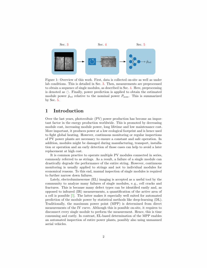
Figure 1: Overview of this work. First, data is collected on-site as well as underlab conditions. This is detailed in Sec. 3. Then, measurements are preprocessedto obtain a sequence of single modules, as described in Sec. 4. Here, preprocessingis denoted as . Finally, power prediction is applied to obtain the estimatedmodule power prel relative to the nominal power Pnom. This is summarizedby Sec. 5.

1 Introduction

Over the last years, photovoltaic (PV) power production has become an impor-tant factor in the energy production worldwide. This is promoted by decreasingmodule cost, increasing module power, long lifetime and low maintenance cost.More important, it produces power at a low ecological footprint and is hence usedto fight global heating. However, continuous monitoring or regular inspectionsof PV power plants are necessary to ensure a constant and safe operation. Inaddition, modules might be damaged during manufacturing, transport, installa-tion or operation and an early detection of those cases can help to avoid a laterreplacement at high cost.

It is common practice to operate multiple PV modules connected in series,commonly referred to as strings. As a result, a failure of a single module candrastically degrade the performance of the entire string. However, continuousmonitoring is usually applied to strings and not to individual modules foreconomical reasons. To this end, manual inspection of single modules is requiredto further narrow down failures.

Lately, electroluminescense (EL) imaging is accepted as a useful tool by thecommunity to analyze many failures of single modules, e. g., cell cracks andfractures. This is because many defect types can be identified easily and, asopposed to infrared (IR) measurements, a quantification of the active area ofa cell is possible [5]. The latter makes it especially well suited for automatedprediction of the module power by statistical methods like deep-learning (DL).Traditionally, the maximum power point (MPP) is determined from directmeasurements of the IV curve. Although this is possible on-site, it requires todisconnect every single module to perform the measurement. Hence, this is timeconsuming and costly. In contrast, EL-based determination of the MPP enablesan automated inspection of entire power plants, possibly also using unmannedaerial vehicles.

2

For PV-plant operators especially cell cracks and fractures with varying origin,including manufacturing process, transport, installation, operating conditions(e. g., storm, hailstorm, snow load) are of particular relevance. Note that,throughout this work, we refer to breaks of the cell that cause parts of itto become disconnected as fractures, whereas cracks are breaks that do notlead to disconnected regions. The impact of cell cracks on the module powerand performance is studied intensely during the last years using EL-images foridentifying cracks and IV-tracers for determining the module power [22, 20, 33, 30,5, 14]. To study crack propagation, mostly climate chambers and static loading,e. g., using sand sacks, were used. Buerhop and Gabor studied the performance ofmodules during static and cyclic loading using a specialized setup [3, 15], whereEL-measurements as well as power data were recorded at loaded and unloadedstages. In addition to the indoor experiments, Buerhop studied the performanceof modules with cracked cells at an on-site test facility in detail [6]. All previousinvestigations have in common that two separate measurements are required:The EL-measurements are used to identify cracks and IV-tracing is used todetermine the power at maximum power point (PMPP). Given that on-site IVmeasurements are costly, an automated and reliable estimation of the PMPPand the impact of cell cracks and fractures on the latter using EL-measurementsare of particular importance for future studies. Note that, throughout thiswork, we use the terms module power and power at maximum power pointinterchangeably.

In a previous conference paper, we showed that the PMPP can be automat-ically predicted from EL measurements taken during indoor mechanical loadtesting experiments [8]. This work is a direct continuation and extension ofthat conference paper. As opposed to the previous work, we now focus onbuilding regression models for on-site data. For efficiency reasons, on-site EL-measurements are usually conducted such that multiple modules are visible in asingle measurement. Since we aim to predict the PMPP for single modules, wedesign a segmentation pipeline for on-site EL-measurements to automaticallygenerate images showing only a single module. Furthermore, we add an extensiveevaluation of the prediction performance, stability and boundary conditions. Fi-nally, we automatically quantify the per cell power loss. The main contributionsof this work are as follows:

(1) We develop a method to predict the PMPP from a single on-site or indoorEL module measurement. We achieve a mean absolute error (MAE) of7.3± 6.5 WP and compare the result against alternative methods in athorough evaluation. Since the dataset is specifically selected such thatmodules have a high shunt resistance, the trained models are restricted tothis defect type.

(2) We propose a fast and robust pipeline to detect and segment multiplemodules in EL measurements, such that item (1) can be directly appliedfor on-site assessment of modules.

(3) We perform an extensive evaluation of boundary conditions, such as mini-

3

mum image size and dataset size.

(4) We set up and publicly release a dataset that is specifically compiled forthe task at hand [7]. In addition, we publish our code and trained models∗,such that a direct application and comparison in future research is feasibleand that our results directly scale to any other PV plant.

(5) We predict the the per cell power loss and analyze the results in termsof defect severity. For our dataset that is compiled such that modulesshow a reduced active area in EL measurements, we find that the PMPPis dominated by fractures and that cracks are only of minor importance.

The remainder of this work is organized as shown in Fig. 1: In Sec. 3, wedescribe the data collection procedure and characterize the dataset used in thiswork. In Sec. 4, we describe the localization of multiple modules from single ELmeasurements. Then, in Sec. 5, we detail the automated power prediction. Thisincludes baseline methods as well as DL-based methods.

Since the different parts of this work are of interest independent of eachother, we decided to summarize the results of every part directly after describingthe methodology and omit a detailed global results section. Then, we finallysummarize the most important results in Sec. 6.

2 Related Work

In the last years, many efforts have been made to leverage computer vision meth-ods in order to reduce the maintenance and operating cost of PV power plants.This includes automated defect analysis for solar cells [37, 25, 9] or automatedprediction of solar irradiance [2]. In prior works, it has been shown that thenumber of cracks visible in EL measurements roughly correlates to the powerloss of a module [12] and that the size of the inactive area on a module correlateswell to the power of the module, as long as the overall fraction of inactive arearemains small [35]. Furthermore, Karimi et al. have shown that the normalizedpower of the module can be determined from various features extracted from theEL image [21]. In addition, there are a few works on PMPP characterizationusing other methods as well. For example, Teubner et al. propose to use IR mea-surements of a module affected by potential induced degradation and computethe PMPP using linear regression from the mean temperature difference of themodule to a reference module [38]. However, this procedure requires that thereference module is exposed to the same environmental conditions (air tempera-ture, wind speed) as the module under test. This is especially challenging forroof-mounted PV installations, where the a temperature gradient is present dueto the convective environment. Furthermore, the measurement accuracy is highlydependent on the available measurement time and steady environmental condi-tions. Recently, Ortega et al. proposed a continuous monitoring of PV powerplants using measurement devices attached to every module [28]. Kropp et al.

∗https://github.com/ma0ho/elpvpower

4

(a) T1 (indoor/on-site) (b) T2 (on-site) (c) T3 (indoor)

Figure 2: Example images from the data set.

manage to predict cell level characteristics from two EL measurements usingsimulations and finally calculate the module power for a single test module [23].

In contrast to the IR-based approach, our method does not require a referencetemperature, since the magnitude of EL measurements mainly depends on cameracharacteristics and the excitation current, which is known in advance. Further, itis based on automated detection of defective areas rather than using module-widestatistics only. In contrast to the measurement-based approach by Ortega et al.,no additional hardware needs to be attached to the modules and the typeand location of a defect can be determined additionally. As opposed to thesimulation-based approach by Kropp et al., our method only requires a single ELmeasurement of a module. In comparison to previous works on power estimationusing a single EL measurement, our method does not rely on hand-craftedfeatures. Instead, relevant features are learned from the data directly, resultingin a data-optimal regression model. Since no manual feature design is required,this method generalizes to various defect and module types, given an appropriatetraining dataset. Furthermore, it enables the visualization of the learned featuresand quantification of per cell or even per defect power losses, facilitating a betterunderstanding for the roots of power degradation.

3 Data

We collected a large set of 719 EL measurements showing 137 module instancesalong with measurements of the maximum power point Pmpp at standard testconditions (1000 W m−2, 25°). The dataset is designed such that it has variationsin the measurement procedure as well as in the type of solar modules. Overall, itcontains three different module types, denoted as T1, T3 and T2 with nominalpowers given by 225 WP to 235 WP, 235 WP to 245 WP and 170 WP to 180 WP

respectively. Furthermore, it also includes variations in the excitation currents,such that models trained using the data should be invariant to the excitationcurrent to some degree. In particular, the excitation current for T3 is given by90%ISC (high current) and 10%ISC (low current), whereas for T2 it is given by

5

0 200 400 600

N

T1 (high) T2 (high)

T2 (low) T3 (high)

T3 (low)

Figure 3: The dataset used in this work consists of three different module types(T1, T3, T2). Two of those have been measured at a high and low current, whichindicated in brackets. Overall, the dataset consists of N = 719 samples.

75%ISC (high current) and 50%ISC (low current). Finally it includes on-sitemeasurements as well as measurements taken at controlled indoor conditions.Examples from the dataset are shown in Fig. 2. The distribution of samplesbetween module types is shown in Fig. 3.

The EL measurements were recorded by a “Greateyes 2048 2048” silicondetector camera with 50 mm focal length lens and a camera triggered powersupply. The camera parameters were fixed for the mechanical load testing siteto an integration time of 5 s and an aperture of 2.4. They measurements havebeen recorded at 16-bit without image compression. Furthermore, the on-sitemeasurements have been taken during night. Here, the integration time was alsofixed to 5 s and the aperture was constant as well.

The PMPP of each PV module was determined from IV-curve measurements.For indoor measurements a table flasher “Spire Spi-Sun Simulator 4600 SLP”with estimated measurement uncertainty of 1.45 % was used, while the indoormeasurements at the mechanical load testing site have been carried out using aprototype of a permanent light source consisting of many halogen lamps. Theresults were extrapolated to standard test conditions (STC) with a measurementuncertainty of 3 % to 4 %. For on-site measurements, a “PVPM 1000CX” with ameasurement uncertainty of at least 5 % according to the data sheet, was used.

As seen from Fig. 3, the dataset is dominated by module type T1, becausethis type has been used for mechanical load testing [4]. During that procedure,load is simulated by an underpressure that is applied on the backside of eachmodule. The underpressure is increased stepwise. After every increase, an ELand PMPP measurement is taken under load. Then, pressure is released andanother set of measurements is taken, before a new load cycle is started. As aresult, there are about 50 sets of measurements of a single module at differentstages of loading including changes in the crack structures. Since these differentstages of degradation come with a variance in PMPP, these load cycles are usefulto assess, if a certain type of defect has an influence on the PMPP. Furthermore,as shown in Fig. 2, there is a series of on-site measurements using module type T1as well.

The set of measurements using module type T2 only consists of on-sitemeasurements. As opposed to T1, we vary the EL excitation current for thismeasurement series between high and low excitation. This is later used to

6

(a) (b) (c) (d)

Figure 4: Preprocessing of multi-module measurements (top: module type T2,bottom: module type T3): Original image (Fig. 4a) is first downsampled andbinarized (Fig. 4b). Next, connected component analysis is applied (Fig. 4c).Finally, bounding boxes of connected components are computed and implausibledetections are rejected (Fig. 4d). Here, rejected detections are depicted by a redbounding box, whereas accepted detections are shown yellow.

obtain a model that performs well irrespective of the excitation current. Thesame holds for module type T3. This module type has been measured underindoor conditions again and includes variations in the excitation current, too.However, this type has not been subject to load testing experiments. Instead, thedegradation is caused by natural events like hailstorms. An even more detailedanalysis of the data can be found in Appendix C.

4 Localization of multiple modules

In this work, we use measurements from multiple sources. These include mea-surements taken under controlled lab conditions, as well as measurements takenon-site. For on-site measurements, it is common practice to capture multiplemodules in a single image in order to reduce the overall number of measure-ments (cf. Fig. 2). In order to assess the power of a single module using thesemeasurements, a localization of module instances is required. We propose afast and straight-forward preprocessing pipeline to locate PV modules in ELmeasurements.

7

4.1 Preprocessing

During preprocessing, we make use of the fact that the background in ELmeasurements has a weak intensity, whereas the modules appear as denselyconnected regions with a high intensity. In addition, modules are usually clearlyseparated by a distinguished margin. Therefore, background and modules areeasily separable by thresholding. We propose a five-step approach:

(1) The original measurement is downscaled by s .

(2) Binarization is performed using Otsu’s method [29]. As a result, themodules are clearly separated (cf. Fig. 4b).

(3) Region candidates are computed by connected component labelling (cf.Fig. 4c) and subsequent region proposal (cf. Fig. 4d) [19].

(4) Final module regions are obtained by rejecting implausible regions that donot adhere to simple constraints (cf. Fig. 4d and Sec. 4.2) and modulesare segmented.

(5) Perspective distortion of module images is removed using the methodproposed by Hoffmann et al. [18].

The downscaling in item (1) is necessary, since the method is based on binarizationand blob detection: Because we only aim at detecting entire modules, smallstructures such as cracks, busbars, cell borders or dirt are not of any interestto the detection at all. However, they regularily cause modules to appear asmultiple seperated blobs in the binarized images, which prevents the accuratedetection of the modules. Fortunately, downscaling the images turned out as anefficient and simple method to counter these effects. At the same time, it speedsup subsequent computations.

4.2 Region constraints

The proposed pipeline results in a large number of false positives. This is due tonoise in the background, parts of a module that are disconnected or modulesthat are only partially visible. The following constraints are applied to rejectfalse positives:

(1) Modules that are not completely visible in the measurement are not ofinterest in this work. Therefore, any detections that touch the boundaryof a measurement are rejected.

(2) Most of the outliers have a very small area, compared to the area of inliers.Therefore, any detections with an area small than τs · amax are rejected.Here, amax refers to the area of the largest detection in a measurementand τs is a hyperparameter.

As a result, we obtain a method that has only two hyperparameters: Thescale s, at which measurements are processed and the minimum area relative tothe maximum area τs.

8

4.3 Experiments

The hyperparameters of this method require proper tuning. To this end, weset up a separate dataset using a total of 37 measurements from the originalon-site measurements. In summary, these measurements show two to sevencompletely visible modules each. We manually annotate bounding boxes forevery completely visible module. Finally, we split the dataset into 25 trainingmeasurements with 75 completely visible modules and 12 test measurementswith 31 modules.

For hyperparameter tuning, we use the Optuna library v1.2 [1] with defaultsettings. Since we are mostly interested in a high detection rate and low falsepositives, we resort to maximizing the F1 score. Here, the F1 score is definedas the harmonic mean of precision and recall. Hence, it jointly accounts for thenumber of false positive and false negative detections. In order to compute theF1 score for a set of detected and ground truth object boxes, it is necessary toassess, if a ground truth box has been detected and, vice versa, if a detectioncorresponds to a ground truth box or is a false positive. To this end, we statethat a module is detected, if the intersection over union (IoU) between detectedand ground truth bounding box is at least τIoU = 0.9. Here, the IoU is defined asthe size of the intersection area divided by the size of the union area between twobounding boxes. Hence, the IoU is maximized, if two bounding boxes overlapperfectly. Then, we calculate the F1 score and perform the optimization onthe training set. Overall, the problem is optimized using 30 trials with thedefault tree-structured Parzen window trial generator. We find that s = 0.23and τs = 0.42 gives the best results on our training split with an F1 score of 1.

4.4 Results

The detection performance on the test split evaluates as F1 = 0.94 using thesame threshold τIoU = 0.9. Detailed results on the detection performance usingdifferent thresholds can be found in Appendix A. We find that the methodperforms very well for τIoU < 0.9 and performs slightly worse for larger valuesof τIoU. However, given that we are mostly interested in a high detection raterather than very accurate detections, the performance is very good. Further, themethod only takes about 322 ms (i7-8650U CPU) for a single image. Please alsonote that this method does not make any assumptions on the number of modulesvisible in a single image. Hence, s is estimated independent of the number ofmodules, although the optimal scale is dependent on the number of modules orthe resolution of a single module.

5 Power prediction

We estimate the power Pmpp at the maximum power point (STC conditions)of a module using a single EL image and the nominal power according tothe data sheet Pnom of the latter. We set up a baseline using support vectorregression (SVR) in Sec. 5.2. We describe our DL-based approach in Sec. 5.3. In

9

order to make the results using SVR and DL comparable, we stick to a commonexperimental procedure, which we describe in Sec. 5.1. Finally, in Sec. 5.4, wecompare both approaches and report experimental results.

Throughout this work, we assume that the nominal power Pnom is known forevery module. Then, we estimate the power relative to Pnom, i. e.,

Pmpp = prel · Pnom (1)

and denote estimates of the relative power prel by prel. Note that, for this dataset,prel roughly correlates to the amount of the inactive area of a module (r = 0.90).While we cannot say, if the slope of a linear model predicting prel from theamount of inactive area is the same for every module type, we expect that theobserved correlation between the two quantities holds for other module typesas well. This is also supported by the work of Schneller et al. that comes to asimilar observation using different data [35].

5.1 Evaluation protocol

The overall goal is to find a model that predicts prel with a low average errorand a small number of outliers. For evaluation purposes, we report the MAEover all samples, as well as the root mean squared error (RMSE). The MAE isgiven by

=1

N

N∑i=1

|p(i)rel − p

(i)rel| (2)

while the RMSE is computed as

=1

N

√√√√ N∑i=1

(p

(i)rel − p

(i)rel

)2

. (3)

Since the dataset is relatively small, making statistically significant statementson model performance using a conventional train/test split of the dataset ishard, since results are necessarily computed on a relatively small test set. Toovercome this limitation, we conduct a cross validation (CV), such that thecomplete dataset is used for testing. We initially split the dataset into 5 foldsusing stratified sampling, such that the overall distribution of relative powers ispreserved between folds. Since a stratified sample requires distinct class labels,we discretize prel in 20 distinct bins, where each bin has a range of 5 %. Further,we make sure that none of the solar module instances ends up in two differentfolds.

The baseline method as well as the DL-based methods have hyperparametersthat need to be tuned properly. In order to enable a fair comparison betweenmethods, we establish a standard protocol. We perform the hyperparameteroptimization using Optuna library v1.2 [1] with the default settings and 250iterations in every fold of the CV to make sure that no test data is used forhyperparameter optimization. Then, we split the training folds into a training

10

and a validation set. While the first one is used to determine model parameters,the latter one is used to optimize hyperparameters. We empirically found thatthe validation set needs to be large enough to obtain stable results. To this end,we use 40 % of the training data for validation. Again, we perform a stratifiedsplit, such that the label-distributions are similar in training and validation set.

5.2 Baseline

In this section, we propose a baseline approach to estimate the Pmpp froma single EL image. We train the SVR using features extracted from the ELmeasurements.

5.2.1 Feature extraction

To apply power estimation using the SVR, we map the data to a low dimensionalfeature representation. This representation is defined such that as much as possi-ble information that is required to estimate the power, is preserved. In previousworks, Zernike moments and Wavelet features have been successfully appliedto recognize textured defects such as cracks on PV modules [24, 13]. However,we know that the power of a module is largely dominated by fractures, sinceour dataset is carefully compiled to adhere to this property. Since fractures aremainly blob-like defects, we use the measurement mean and standard deviation,which is a good representation for that. Furthermore, it has been shown thatfeatures extracted from models pretrained on the ImageNet [10] dataset areuseful for machine learning tasks on different data as well [26, 36]. Therefore,we include features extracted from a pretrained ResNet18 as well [16]. TheResNet architecture has become popular for many computer vision problems. Itis available in different configurations featuring between 18 and 152 layers. It wasthe first architecture that introduced residual connections between subsequentlayers, which mainly solved the issue of vanishing gradients. As a result, itenables to increase the number of layers of a DL architecture. To compute theResNet18-features fR18, we convert measurements into RGB images and performchannel-wise normalization using the per-channel statistics. Hence, we makesure that the statistics of the measurements match those of the ImageNet [10]dataset that has been used during training. For the pretrained ResNet18, weuse the model available in the open-source DL framework PyTorch v1.3 [31] anddrop the fully connected layer to obtain features directly after global averagepooling. On the other hand, the features composed of the mean and standarddeviation of intensities fµ,σ is computed without further preprocessing.

The feature extraction is followed by a normalization. Here, we compute themean and standard deviation of every feature independently using all samplesfrom the training data. We use these statistics to normalize training, as well astest features.

11

indoor on-site T1 T2 T3 high current low current

100 200

100

200

Pmpp[W

P]

SVR fµ,σMAE: 9.0 ± 8.4WP

100 200

SVR fR18MAE: 10.6 ± 9.9WP

100 200

100

200

Pmpp [WP]

Pmpp[W

P]

MobileNetV2MAE: 7.8 ± 7.5WP

100 200

Pmpp [WP]

ResNet18MAE: 7.3 ± 6.5WP

100 200

Pmpp [WP]

ResNet50MAE: 10.5 ± 9.7WP

Figure 5: Distribution of estimation errors of all methods. We aggregate theresults from all folds of the cross validation (CV), such that all samples ofthe dataset are shown here. For the samples, we distinguish between indoorand on-site measurements by marker shape. Further, we distinguish betweenmodule type T1 , T2 and T3 by marker color. Finally, we differentiatemeasurements taken at high current or low current by marker filledness. Forbetter visualization, the ideal regression line is shown . Furthermore,indicates the 0± 15 WP isoline.

12

5.2.2 Experimental procedure

The SVR regression aims to minimize the absolute regression error

|∆prel| = |prel − prel| (4)

for those samples that have ∆prel > ε, while maintaining a regression modelwith a small Lipschitz constant. Here, ε is the width of the epsilon-tube withinwhich errors do not contribute to the loss of the SVR objective function [11].We use the implementation from the Scikit-learn library v0.20 [32] with thedefault radial basis function kernel. For the width of the epsilon-tube and theregularization constant, we conduct a hyperparameter optimization in every foldas described in Sec. 5.1.

5.3 Deep-learning

In this section, we introduce the DL-based approach to predict Pmpp given anEL-measurement as well as the nominal power Pnom of the module. We presenta straightforward approach and use standard DL-architectures that have beentrained on ImageNet [10] to perform regression of prel (see Eq. (1)). We detailour methodology in Sec. 5.3.1 and focus on the pipeline that empirically workedbest. In Sec. 5.3.2 we explain, how we tuned the hyperparameters for differentDL-models.

5.3.1 Method

As deep neural networks (DNNs) are usually trained end-to-end, meaning thatthe feature extraction is part of the training process, there are only a few designchoices that need to be made. These include (1) the preprocessing that is appliedto the raw measurements (2) the DL-models that are used (3) the loss function(4) the optimization method. We detail our choices in the next paragraphs:

Preprocessing Although we only use fully-convolutional networks, it is com-mon to limit the resolution of input measurements to reduce the computationaleffort. We rescale measurements such that the smallest side equals 800 px. Then,we normalize the measurements using the common normalization with globalstatistics. To this end, we compute the mean µ and standard deviation σ ofphoton counts using our data. A sample x is then normalized according to

x′ =x− µσ

. (5)

The choices of scale and normalization scheme are verified by initial experimentsreported in Fig. 6.

Furthermore, we apply online data augmentation during training. As alreadyreported by Deitsch et al. [9] for the case of single cells, light data augmentationis sufficient, since the segmented modules are mostly fixed in orientation andposition due to the module detection and removal of perspective distortion.

13

200 400 600 800 1,000

2

4

6

scale [px]

MAE

[%]

(a) Sensitivity of the error with respect tovariations in measurement scale.

20 30 40

2

3

4

5

epochs

global std.measurement std.ZCA whitening

(b) Sensitivity of the error with re-spect to variations in the normalizationscheme.

Figure 6: We conduct a series of initial experiments to determine the bestmeasurement scale and normalization scheme. All experiments were performedusing ResNet18 without further hyperparameter tuning. Every model is trained5 times until convergence. We report the minimum MAE on the validation set.Error bars denote the standard deviation of the MAE between training runs.In Sec. 5.3.1, we scale the smallest side of the measurement to the specifiedvalue. In Sec. 5.3.1, we compare the common global normalization, whereall measurements are normalized by the same statistics computed over thewhole training set to a measurement-wise approach, where every measurementis normalized using it’s own statistics. Finally, we include normalization bypatch-wise zero component analysis (ZCA)-whitening. It turns out that a scaleof 800 px and the common global normalization give the best results.

We apply random horizontal and vertical flips, random rotation by at most±10, random translation by 5% of the image size at maximum and randomdownscaling to 80% of the image size at minimum. The augmented images arezero-padded to match the original image size.

DL models In many recent works, it has been shown that applying transferlearning is advantageous over training models from scratch, even if source andtarget domain differ [39]. Therefore, we resort to using standard architectures,where pretrained weights are readily available. In this work, we focus on threedifferent architectures: First, we include a small and a larger network fromthe ResNet architecture family (ResNet18 and ResNet50) [16]. This allows usto investigate, if deeper architectures are beneficial for the task at hand. Inaddition, we include the MobileNetV2 architecture [34], which is specificallydesigned for high throughputs at inference time, since this is a major benefit for

14

practical applications.For every one of those models, the final layer is composed by a matrix

multiplication that maps the high dimensional feature representation to thecorrect output size. This layer is often referred to as the fully connected (FC)layer. We replace the final FC layer by a randomly initialized FC layer witha single output. We do not perform any non-linear activation on the output.Hence, this corresponds to a linear regression of prel using the features fromprevious layers.

Loss function Common loss functions for regression problems include themean squared error (MSE) and MAE. By definition, MSE puts a higher weighton outliers, resulting in a model that performs better for underrepresented casesand worse for overrepresented cases. Since we are interested in a model thatperforms well over a large range of samples, we minimize the MSE.

Optimization A huge variety of optimization methods has been proposed inthe literature. For this work, we decided to use some of the most prevalentapproaches: We use stochastic gradient descent (SGD) with momentum ν = 0.9and weight decay λ and properly tune the learning rate η, batch size B andweight decay λ independently for every architecture. For the learning rateschedule, we reduce the learning rate as soon as the validation loss does notdecrease for 20 epochs. Here, an epoch refers to training once on the completetraining dataset.

5.3.2 Experimental procedure

Proper tuning of hyperparameters is crucial in order to perform a fair comparisonof different architectures. We use the Optuna library v1.2 [1] to determine theoptimal values for η, B and λ individually for every architecture and fold of theCV, as described in Sec. 5.1. The results are summarized by Tab. 1. We findthat optimal parameters are relatively similar across architectures.

As soon as the optimal hyperparameters are determined, we use them totrain a final model for every fold that is then tested using the test data of therespective fold. As opposed to the hyperparameter search, we now use 80 %of the data for training and only 20 % for validation. We further apply earlystopping after 40 epochs without improvement on the validation set and use thecheckpoint that performed best on the validation set for testing.

5.4 Results

In this section, we assess the performance of the architectures for the predictionof PMPP and compare it to the performance of the baseline model. By training5 CV folds with every architecture using the parameters found by hyperparameteroptimization, we assess the stability of every method with respect to variationsin the training and test data. We report the results on the test folds in Fig. 7and in Tab. 2. It turns out that ResNet18 and MobileNetV2 have a smaller

15

SVR fµ,σ SVR fR18 MobileNetV2 ResNet18 ResNet50

0

5

10

15

|∆prel|[%

]outlier

Figure 7: Distributions of sample errors over all 5 folds of the CV. The errorsare computed on the testset of every fold. Note that the y axis has been cut at|∆prel| = 15% for better visualization.

average MAE than the baseline, whereas ResNet50 does not perform well. Thisis explained by the relatively small dataset. Among the SVR-based methods,fµ,σ has the lowest MAE. However, it also shows the strongest variation betweenfolds, indicating that the result is very data dependent. Overall, ResNet18 givesthe lowest MAE and RMSE.

In terms of variation between CV folds, ResNet50 turns out most stable.However, the advantage over ResNet18 is neglectible. We observe that the gapbetween MAE and RMSE is smaller for the DL-based models compared to theSVR-based ones. This is explained by the difference in the loss function, sinceSVR roughly minimizes the MAE (cf. Eq. (4)), whereas we chose to minimizethe MSE for the DL-based models.

In Fig. 5, we show the distribution of errors for all samples in the dataset andall methods. This is obtained by merging all five test folds into a single figure.The comparison shows that the predictions of ResNet18 are well aligned with theideal regression line, whereas the predictions using SVR are skewed with respectto the ideal line. We conclude that this is caused by the features chosen for theregression model that do not result in a linear regression problem under the RBFkernel. However, initial experiments with other kernels performed even worse.We also compute the p-value using a t-test to assess, if the ResNet18 performssignificantly better than the other approaches. We find that the performancedifference to the MobileNetV2 is not statistically significant, whereas ResNet18performs significantly better than the remaining other methods (p < 0.0001).

Finally, in Tab. 3, we summarize the results for different subsets of the data.It turns out that the prediction is stable across most of the different subsets.The only exception are those modules measured at a low excitation current and

16

B λ η

MobileNetV2 8 1.00± 1.01× 10−2 3.54± 11.30× 10−3

ResNet18 8 2.59± 0.69× 10−2 3.41± 5.70 × 10−3

ResNet50 8 1.79± 2.44× 10−2 3.38± 8.80 × 10−3

Table 1: Results from the hyperparameter optimization using Optuna li-brary v1.2 [1]. The hyperparameter optimization has been performed using250 iterations per model. We optimize the the batch size sampling fromB ∈ [8, 16, 32, 64], the learning rate sampling from η ∈

[1× 10−5, 1× 10−1

]and the weight decay sampling from λ ∈

[1× 10−3, 1× 10−1

]in logspace. Sam-

pling is performed using the default tree-structured Parzen window approachand unsuccessful trials are pruned.

MAE [%] RMSE [%] MAE [WP] RMSE [WP]

MobileNetV2 3.4± 3.2 4.7 7.8± 7.5 4.7ResNet18 3.2± 2.7 4.2 7.3± 6.5 4.2ResNet50 4.5± 4.1 6.2 10.5± 9.7 6.2SVR fµ,σ 4.0± 3.7 5.5 9.0± 8.4 5.5SVR fR18 4.6± 4.2 6.2 10.6± 9.9 6.2

Table 2: Quantitative results computed by CV. We show the MAE and theRMSE averaged over the test sets of every fold of the CV. In addition, thestandard deviation of errors is shown. Finally, we explicitly show the relativeerror, as used in training as well as the absolute error in [WP] for betterinterpretability.

modules of type T3. Both of them perform worse than the others. Subset T3 iscomposed of modules measured at high and low current. Hence, it contains thesame modules twice. We find that modules from subset T3 that are measured athigh current result in a MAE of 4.3 %, whereas modules from the same subsetmeasured at a low current result in a MAE of 4.7 %. Specifically, modules fromsubset T3 are mostly underestimated and we find that this effect is more severefor modules measured at a low current. Since those results have been computedusing the same module instances and are averaged over all 5 folds of the CV, wecan conclude that the model performs slightly better on measurements taken ata high current, irrespective of the module type. However, this result might bebiased by the fact that the dataset is largely dominated by samples measured ata high current.

5.4.1 Visualization of Class Activation Maps

In previous works, it has been shown that object locations can be extracted fromDNNs trained for object classification [27]. To this end, the activation mapsfrom the last layer that preserves spatial information are used to calculate a

17

MAE [%] RMSE [%] MAE [WP] RMSE [WP] N

indoor 3.1± 2.8 4.1 7.1± 6.6 9.7 596on-site 3.6± 2.7 4.5 8.1± 6.2 10.1 123high current 3.0± 2.7 4.0 6.9± 6.2 9.3 646low current 4.5± 3.3 5.5 10.3± 8.0 13.0 73T1 2.7± 2.6 3.7 6.2± 6.0 8.6 478T2 2.6± 1.8 3.1 4.5± 3.2 5.5 28T3 4.6± 3.1 5.5 11.0± 7.5 13.3 118

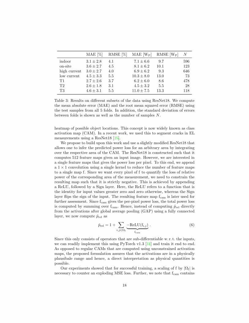
Table 3: Results on different subsets of the data using ResNet18. We computethe mean absolute error (MAE) and the root mean squared error (RMSE) usingthe test samples from all 5 folds. In addition, the standard deviation of errorsbetween folds is shown as well as the number of samples N .

heatmap of possible object locations. This concept is now widely known as classactivation map (CAM). In a recent work, we used this to segment cracks in ELmeasurements using a ResNet18 [25].

We propose to build upon this work and use a slightly modified ResNet18 thatallows one to infer the predicted power loss for an arbitrary area by integratingover the respective area of the CAM. The ResNet18 is constructed such that itcomputes 512 feature maps given an input image. However, we are interested ina single feature maps that gives the power loss per pixel. To this end, we appenda 1× 1 convolution using a single kernel to reduce the number of feature mapsto a single map f. Since we want every pixel of f to quantify the loss of relativepower of the corresponding area of the measurement, we need to constrain theresulting map such that it is strictly negative. This is achieved by appendinga ReLU, followed by a Sign layer. Here, the ReLU refers to a function that isthe identity for input values greater zero and zero otherwise, whereas the Signlayer flips the sign of the input. The resulting feature map fcam is later used forfurther assessment. Since fcam gives the per-pixel power loss, the total power lossis computed by summing over fcam. Hence, instead of computing prel directlyfrom the activations after global average pooling (GAP) using a fully connectedlayer, we now compute prel as

prel = 1 +∑i,j∈Ωf

−ReLU(fi,j)︸ ︷︷ ︸fcam

. (6)

Since this only consists of operators that are sub-differentiable w. r. t. the inputs,we can readily implement this using PyTorch v1.3 [31] and train it end to end.As opposed to regular CAMs that are computed using unconstrained activationmaps, the proposed formulation assures that the activations are in a physicallyplausibale range and hence, a direct interpretation as physical quantities ispossible.

Our experiments showed that for successful training, a scaling of f by |Ωf | isnecessary to counter an exploding MSE loss. Further, we note that fcam contains

18

−0.6 −0.4 −0.2 −0.2 −0.5 −0.2 −0.1 −0.3 −0.4 −0.2

−0.2 −0.3 −1.7 −0.8 −1.0 −1.3 −0.1 −0.5 −0.3 −0.4

−0.3 −0.3 −0.7 −0.2 −0.2 −0.4 −0.3 −0.2 −0.1 −1.0

−0.1 −0.3 −0.3 −0.1 −0.1 −0.1 −0.4 −0.3 −0.1 −0.3

−0.3 −1.2 −1.5 −0.5 −1.8 −1.1 −1.5 −2.3 −0.3 −0.5

−0.3 −0.9 −0.7 −0.6 −0.6 −1.5 −0.8 −0.9 −0.8 −0.9

0

25

50

75

100

[%]

Figure 8: Visualization of class activation map (CAM) using a modified ResNet18.Note that we color-code the original EL measurement with the given colormapusing the relative magnitude of −fcam such that brighter colors correspond toregions with high relative power loss. Since the intensity is given by the originalmeasurement, color appearence does not exactly correspond to the legend, sincethe legend uses a linear intensity ramp. For every cell, we give the power lossdetermined by the model in WP. This is computed by integrating over thecorresponding area of the CAM, resulting in the relative power loss, which isconverted into the absolute power loss by Eq. (1).

a small constant bias after training. We remove that bias by subtracting themedian of multiple fcam computed from module images with prel ≈ 1 from allfcam.

The results are shown in Fig. 8 and additional examples can be foundin Appendix B. It turns out that the resulting CAMs mostly highlight thefractures, indicating that the network is able to learn physically relevant featuresand that fractures are the main source of power loss as opposed to cracks.

It becomes apperent that, in many examples, the amount of power loss percell predicted by the network is roughly proportional to the amount of inactivearea. Although this might appear obvious at first, this is not a trivial finding,because there are various types of cracks and their relative position is importantas well. For example, it is known that the current and with the the power of astring is limited by the worst cell, since all cells are connected in series. However,at least for this dataset, the network reveals a linear relationship between theamount of inactive area and module power. To verify this, we compute the sizeof inactive area for every module in the dataset by thresholding and calculate thepower loss proportional to the inactive area, which is similar to the thresholding

19

100 200

100

200

Pmpp [WP]

Pmpp[W

P]

SVR fµ,σ

100 200

Pmpp [WP]

SVR fR18

100 200

Pmpp [WP]

ResNet18

Figure 9: Distribution of estimation errors for the generalization experiment.For the samples, we distinguish between indoor and on-site measurements bymarker shape. Further, we distinguish between module type T2 and T3 bymarker color. Finally, we differentiate measurements taken at high current orlow current by marker filledness. For better visualization, the ideal regressionline is shown . Furthermore, indicates the 0± 15 WP isoline.

MAE [%] RMSE [%] MAE [WP] RMSE [WP]

ResNet18 9.5± 6.0 11.3 22.6± 14.8 27.0SVR fµ,σ 14.8± 11.4 18.6 34.0± 27.9 43.9SVR fR18 17.1± 10.0 19.8 39.3± 24.8 46.4

Table 4: Quantitative results of the generalization experiment. We show theMAE and the RMSE as well as the standard deviation of errors. Finally, weexplicitly show the relative error, as used in training as well as the absolute errorin [WP] for better interpretability.

approach by Schneller et al. [35]. Using this approach, the module power ispredicted with a MAE of 8.5± 2.1 WP, which is on par with the baseline resultsreported in Fig. 7. It is possible that those results could be improved evenfurther by using more than a single threshold, because this would allow themodel to take variations in the shunt resistance into account.

5.5 Generalization to unseen Data

Finally, we aim to assess, if the method generalizes well to module types thathave not been used during training. This experiment is conducted using theResNet18, since this performed best in the previous experiments. In addition, weinclude the SVR-based methods for reference. We train the model on samples T1using the hyperparameters that have been found in the first fold of the CV andtest on samples T2 and T3. Note that the module types differ in their physical

20

properties. For example, T1 and T3 consist of 10 × 6 polycrystalline cells, ofwhich each has an edge length of 6 inch, whereas T2 consists of 12× 6 cells withan edge length of 5-inch. Furthermore, they also differ in their nominal power,which is given as 230 WP for T1, 170 WP for T2 and 240 WP for T3. However,all types have in common that their cells are arranged in 3 substrings that areconnected in parallel and include a bypass diode for every substring.

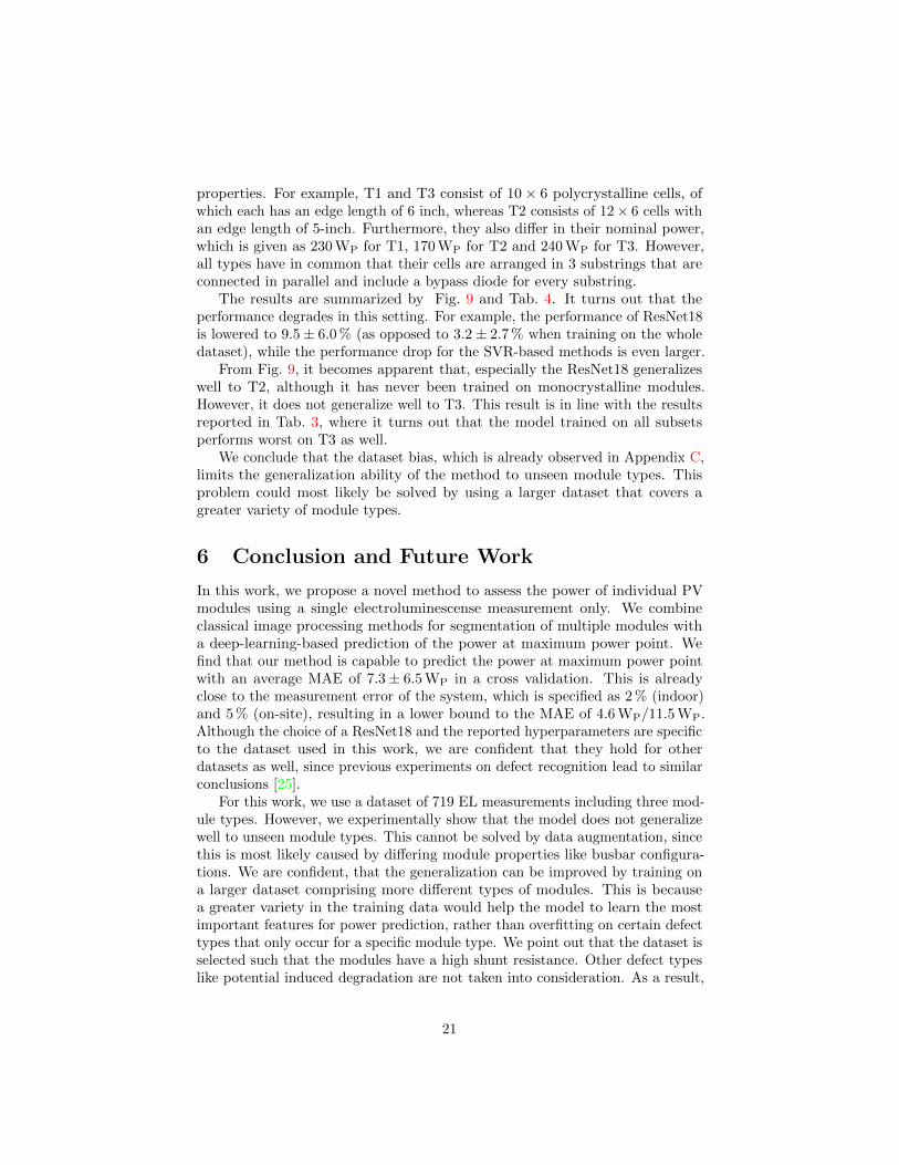
The results are summarized by Fig. 9 and Tab. 4. It turns out that theperformance degrades in this setting. For example, the performance of ResNet18is lowered to 9.5± 6.0 % (as opposed to 3.2± 2.7 % when training on the wholedataset), while the performance drop for the SVR-based methods is even larger.

From Fig. 9, it becomes apparent that, especially the ResNet18 generalizeswell to T2, although it has never been trained on monocrystalline modules.However, it does not generalize well to T3. This result is in line with the resultsreported in Tab. 3, where it turns out that the model trained on all subsetsperforms worst on T3 as well.

We conclude that the dataset bias, which is already observed in Appendix C,limits the generalization ability of the method to unseen module types. Thisproblem could most likely be solved by using a larger dataset that covers agreater variety of module types.

6 Conclusion and Future Work

In this work, we propose a novel method to assess the power of individual PVmodules using a single electroluminescense measurement only. We combineclassical image processing methods for segmentation of multiple modules witha deep-learning-based prediction of the power at maximum power point. Wefind that our method is capable to predict the power at maximum power pointwith an average MAE of 7.3± 6.5 WP in a cross validation. This is alreadyclose to the measurement error of the system, which is specified as 2 % (indoor)and 5 % (on-site), resulting in a lower bound to the MAE of 4.6 WP/11.5 WP.Although the choice of a ResNet18 and the reported hyperparameters are specificto the dataset used in this work, we are confident that they hold for otherdatasets as well, since previous experiments on defect recognition lead to similarconclusions [25].

For this work, we use a dataset of 719 EL measurements including three mod-ule types. However, we experimentally show that the model does not generalizewell to unseen module types. This cannot be solved by data augmentation, sincethis is most likely caused by differing module properties like busbar configura-tions. We are confident, that the generalization can be improved by training ona larger dataset comprising more different types of modules. This is becausea greater variety in the training data would help the model to learn the mostimportant features for power prediction, rather than overfitting on certain defecttypes that only occur for a specific module type. We point out that the dataset isselected such that the modules have a high shunt resistance. Other defect typeslike potential induced degradation are not taken into consideration. As a result,

21

the trained models are restricted to this particular type of defects. However,we are confident that the method can be applied to other defect types as well,as long as they are visible in EL measurements and a comprehensive trainingdataset is available.

We transfer the concept of class activation maps to the regression task anduse it to calculate the power loss per cell jointly with the power loss of theoverall module. Since the per cell power loss has never been used during training,this approach allows to quantify the impact of individual defects on the overallpower output and does not require any additional measurements or finite elementanalysis. Our experiments show that the model can automatically determine thedefect types that are most relevant to calculate the power loss of the module.By means of the thresholding experiment, we show that this quantification ofpower losses can help to design simpler methods that only perform slightly worse,compared to the DL-based approach.

Furthermore, we compile and release the dataset consisting of 719 EL measure-ments that have been aquired under varying conditions as well as measurementsof the Pmpp at standard test conditions. This includes indoor and on-site mea-surements as well as measurements from load cycle experiments. As some of theon-site measurements show multiple modules at the same time, we propose asimple yet robust preprocessing pipeline to detect and segment module instances.We evaluate the detection of modules on a separate testset and find that itresults in a detection rate of F1 = 0.94. This detection pipeline is currentlydesigned to detect modules that do not have a defective substring. Modules witha defective substring result in two separate detections, since the parts are notconneceted in the binarized measurement. An extension of the method for suchcases is subject to future works.

For future works, we think that it might be interesting to consider architec-tures that operate on cell level, because they could take the electrical connectionsinto account, which is not considered in this work. As shown in Sec. 5.4.1, themodel mainly focusses on fractures, which is consistent to physical considerationsand prior works. However, the impact of a fracture on the PMPP is dependenton the overall conductivity of the substring. This relationship could be learnedfrom the data using an architecture that determines the fraction of inactivearea per cell and subsequently combines this information into a final estimate.Further, the generalization gap shown in Fig. 9 deserves further investigation.

We are confident that this work contributes to an automated and contactlessassessment of large PV power plants. By releasing the data and code, we aim toallow other researchers to reproduce our results and to push the field forward.

Acknowledgements

We gratefully acknowledge the BMWi as well as the IBC SOLAR AG for financialfunding of the project iPV4.0 (FKZ: 0324286) and the German Federal Ministryfor Economic Affairs and Energy (BMWi) for financial funding of the projectCOSIMA (FKZ: 032429A). Furthermore, we acknowledge the PV-Tera grant bythe Bavarian State Government (No. 44-6521a/20/5). Further, we thank Allianz

22

Risk Consulting GmbH / Allianz Zentrum fur Technik (AZT) for providing uswith a large number of PV modules.

23

References

[1] Takuya Akiba, Shotaro Sano, Toshihiko Yanase, Takeru Ohta, and MasanoriKoyama. Optuna: A next-generation hyperparameter optimization frame-work. In Proceedings of the 25th ACM SIGKDD International Conferenceon Knowledge Discovery & Data Mining, pages 2623–2631, 2019.

[2] David Bernecker, Christian Riess, Elli Angelopoulou, and Joachim Horneg-ger. Continuous short-term irradiance forecasts using sky images. SolarEnergy, 110:303–315, 2014.

[3] C Buerhop, T Winkler, T Patel, J Hauch, C Camus, and CJ Brabec.Performance analysis of pre-cracked pv modules at cyclic loading conditions.In 35th EU PVSEC, page 1554, 2018.

[4] C. Buerhop, S. Wirsching, S. Gehre, T. Pickel, T. Winkler, A. Bemm,J. Mergheim, C. Camus, J. Hauch, and C. J. Brabec. Lifetime and degra-dation of pre-damaged pv-modules – field study and lab testing. In 2017IEEE 44th Photovoltaic Specialist Conference (PVSC), pages 3500–3505,2017.

[5] Claudia Buerhop, Sven Wirsching, Andreas Bemm, Tobias Pickel, PhilippHohmann, Monika Nieß, Christian Vodermayer, Alexander Huber, BernhardGluck, Julia Mergheim, et al. Evolution of cell cracks in pv-modules underfield and laboratory conditions. Progress in Photovoltaics: Research andApplications, 26(4):261–272, 2018.

[6] C Buerhop-Lutz, T Winkler, FW Fecher, A Bemm, J Hauch, C Camus,and CJ Brabec. Performance analysis of pre-cracked pv-modules at realisticloading conditions. Proceedings of the 33rd European PV-SEC, 5CO, 8:1451–1456, 2017.

[7] Claudia Buerhop-Lutz and Mathis Hoffmann. ELPVPower: A dataset forlarge scale PV power prediction using EL images, 2020.

[8] Claudia Buerhop-Lutz, Mathis Hoffmann, Luca Reeb, Tobias Pickel, JensHauch, and Andreas Maier. Applying Deep Learning Algorithms to EL-images for Predicting the Module Power. In Proceedings of the 36th EuropeanPhotovoltaic Solar Energy Conference and Exhibition, pages 858 – 863, 2019.

[9] Sergiu Deitsch, Vincent Christlein, Stephan Berger, Claudia Buerhop-Lutz,Andreas Maier, Florian Gallwitz, and Christian Riess. Automatic classifica-tion of defective photovoltaic module cells in electroluminescence images.Solar Energy, 185:455–468, 2019.

[10] Jia Deng, Wei Dong, Richard Socher, Li-Jia Li, Kai Li, and Li Fei-Fei. Ima-genet: A large-scale hierarchical image database. In 2009 IEEE conferenceon computer vision and pattern recognition, pages 248–255. Ieee, 2009.

24

[11] Harris Drucker, Christopher JC Burges, Linda Kaufman, Alex J Smola,and Vladimir Vapnik. Support vector regression machines. In Advances inneural information processing systems, pages 155–161, 1997.

[12] Rajiv Dubey, Shashwata Chattopadhyay, Sachin Zachariah, Sugguna Ram-babu, K Hemant, Singh Anil Kottantharayil, Brij M Arora, KL Narasimhan,Narendra Shiradkar, and Juzer Vasi. On-site electroluminescence study offield-aged pv modules. In 2018 IEEE 7th World Conference on PhotovoltaicEnergy Conversion (WCPEC)(A Joint Conference of 45th IEEE PVSC,28th PVSEC & 34th EU PVSEC), pages 0098–0102. IEEE, 2018.

[13] F. Farress, A. El Hassani Alaoui, M.N. Saidi, A. Tamtaoui, Z. Zaimi, andA. Bennouna. Defect detection in solar cells using electroluminescenceimaging and image processing algorithms. volume 8, 2017.

[14] Andrew M. Gabor, Rob Janoch, Andrew Anselmo, and Halden Field. Solarpanel design factors to reduce the impact of cracked cells and the tendencyfor crack propagation. In 2015 NREL PV Module Reliability Workshop.

[15] Andrew M Gabor, Rob Janoch, Andrew Anselmo, Jason L Lincoln, HubertSeigneur, and Christian Honeker. Mechanical load testing of solar pan-els—beyond certification testing. In 2016 IEEE 43rd Photovoltaic SpecialistsConference (PVSC), pages 3574–3579. IEEE, 2016.

[16] Kaiming He, Xiangyu Zhang, Shaoqing Ren, and Jian Sun. Identity map-pings in deep residual networks. In European conference on computer vision,pages 630–645. Springer, 2016.

[17] Geoffrey E Hinton and Sam T Roweis. Stochastic neighbor embedding. InAdvances in neural information processing systems, pages 857–864, 2003.

[18] Mathis Hoffmann, Bernd Doll, Florian Talkenberg, Christoph J Brabec,Andreas K Maier, and Vincent Christlein. Fast and robust detection ofsolar modules in electroluminescence images. In International Conferenceon Computer Analysis of Images and Patterns, pages 519–531. Springer,2019.

[19] Bernd Jahne. Digitale Bildverarbeitung. Springer, 2013.

[20] Sarah Kajari-Schroder, Iris Kunze, Ulrich Eitner, and Marc Kontges. Spatialand orientational distribution of cracks in crystalline photovoltaic modulesgenerated by mechanical load tests. Solar Energy Materials and Solar Cells,95(11):3054–3059, 2011.

[21] Ahmad Maroof Karimi, Justin S Fada, Nicholas A Parrilla, Benjamin GPierce, Mehmet Koyuturk, Roger H French, and Jennifer L Braid. Gener-alized and mechanistic pv module performance prediction from computervision and machine learning on electroluminescence images. IEEE Journalof Photovoltaics, 10(3):878–887, 2020.

25

[22] M Kontges, S Kajari-Schroder, I Kunze, and U Jahn. Crack statistic ofcrystalline silicon photovoltaic modules. In 26th EU PVSEC, volume 26,pages 3290–3294, 2011.

[23] Timo Kropp, Markus Schubert, and Jurgen H Werner. Quantitative predic-tion of power loss for damaged photovoltaic modules using electrolumines-cence. Energies, 11(5):1172, 2018.

[24] Wei-Chen Li and Du-Ming Tsai. Wavelet-based defect detection in solarwafer images with inhomogeneous texture. Pattern Recognition, 45(2):742–756, 2012.

[25] Martin Mayr, Mathis Hoffmann, Andreas Maier, and Vincent Christlein.Weakly supervised segmentation of cracks on solar cells using normalized l pnorm. In 2019 IEEE International Conference on Image Processing (ICIP),pages 1885–1889. IEEE, 2019.

[26] Maxime Oquab, Leon Bottou, Ivan Laptev, and Josef Sivic. Learningand transferring mid-level image representations using convolutional neuralnetworks. In Proceedings of the IEEE conference on computer vision andpattern recognition, pages 1717–1724, 2014.

[27] Maxime Oquab, Leon Bottou, Ivan Laptev, and Josef Sivic. Is objectlocalization for free?-weakly-supervised learning with convolutional neuralnetworks. In Proceedings of the IEEE conference on computer vision andpattern recognition, pages 685–694, 2015.

[28] Eneko Ortega, Gerardo Aranguren, and Juan Carlos Jimeno. New monitor-ing method to characterize individual modules in large photovoltaic systems.Solar Energy, 193:906–914, 2019.

[29] Nobuyuki Otsu. A threshold selection method from gray-level histograms.IEEE transactions on systems, man, and cybernetics, 9(1):62–66, 1979.

[30] Marco Paggi, Mauro Corrado, and Irene Berardone. A global/local ap-proach for the prediction of the electric response of cracked solar cells inphotovoltaic modules under the action of mechanical loads. EngineeringFracture Mechanics, 168:40–57, 2016.

[31] Adam Paszke, Sam Gross, Francisco Massa, Adam Lerer, James Bradbury,Gregory Chanan, Trevor Killeen, Zeming Lin, Natalia Gimelshein, LucaAntiga, et al. Pytorch: An imperative style, high-performance deep learninglibrary. In Advances in Neural Information Processing Systems, pages8024–8035, 2019.

[32] Fabian Pedregosa, Gael Varoquaux, Alexandre Gramfort, Vincent Michel,Bertrand Thirion, Olivier Grisel, Mathieu Blondel, Peter Prettenhofer, RonWeiss, Vincent Dubourg, et al. Scikit-learn: Machine learning in python.Journal of machine learning research, 12(Oct):2825–2830, 2011.

26

[33] M Sander, S Dietrich, M Pander, S Schweizer, M Ebert, and J Bagdahn.Investigations on crack development and crack growth in embedded solarcells. In Reliability of Photovoltaic Cells, Modules, Components, and Sys-tems IV, volume 8112, page 811209. International Society for Optics andPhotonics, 2011.

[34] Mark Sandler, Andrew Howard, Menglong Zhu, Andrey Zhmoginov, andLiang-Chieh Chen. Mobilenetv2: Inverted residuals and linear bottlenecks.In Proceedings of the IEEE conference on computer vision and patternrecognition, pages 4510–4520, 2018.

[35] Eric J Schneller, Rafaela Frota, Andrew M Gabor, Jason Lincoln, HubertSeigneur, and Kristopher O Davis. Electroluminescence based metrics to as-sess the impact of cracks on photovoltaic module performance. In 2018 IEEE7th World Conference on Photovoltaic Energy Conversion (WCPEC)(AJoint Conference of 45th IEEE PVSC, 28th PVSEC & 34th EU PVSEC),pages 0455–0458. IEEE, 2018.

[36] Ali Sharif Razavian, Hossein Azizpour, Josephine Sullivan, and StefanCarlsson. Cnn features off-the-shelf: an astounding baseline for recognition.In Proceedings of the IEEE conference on computer vision and patternrecognition workshops, pages 806–813, 2014.

[37] Daniel Stromer, Andreas Vetter, Hasan Can Oezkan, Christian Probst, andAndreas Maier. Enhanced crack segmentation (ecs): A reference algorithmfor segmenting cracks in multicrystalline silicon solar cells. IEEE Journalof Photovoltaics, 2019.

[38] Janine Teubner, Claudia Buerhop, Tobias Pickel, Jens Hauch, ChristianCamus, and Christoph J Brabec. Quantitative assessment of the powerloss of silicon pv modules by ir thermography and its dependence on data-filtering criteria. Progress in Photovoltaics: Research and Applications,27(10):856–868, 2019.

[39] Jason Yosinski, Jeff Clune, Yoshua Bengio, and Hod Lipson. How transfer-able are features in deep neural networks? In Advances in neural informationprocessing systems, pages 3320–3328, 2014.

27

Appendices

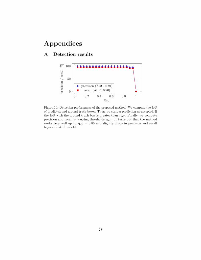
A Detection results

0 0.2 0.4 0.6 0.8 1

0

50

100

τIoU

precision

/recall[%

]

precision (AUC: 0.94)

recall (AUC: 0.90)

Figure 10: Detection performance of the proposed method. We compute the IoUof predicted and ground truth boxes. Then, we state a prediction as accepted, ifthe IoU with the ground truth box is greater than τIoU. Finally, we computeprecision and recall at varying thresholds τIoU. It turns out that the methodworks very well up to τIoU = 0.85 and slightly drops in precision and recallbeyond that threshold.

28

B Additional CAMs

−2.0 −0.5 −0.7 −0.3 −0.0 −0.1 −0.1 −0.0 −0.0 −0.6

−0.5 −0.4 −1.0 −0.3 −0.0 −0.0 −0.1 −0.0 −0.1 −0.4

−0.1 −0.1 −0.0 −0.0 −0.1 −0.2 −0.3 −0.3 −0.5 −0.4

−0.1 −0.0 −0.0 −0.0 −0.4 −1.2 −1.9 −1.0 −0.4 −0.2

−0.1 −0.2 −1.3 −0.1 −0.3 −0.7 −2.2 −0.7 −0.0 −0.4

−0.5 −1.7 −0.9 −0.5 −1.9 −1.8 −1.9 −1.5 −0.1 −0.5

0

25

50

75

100

[%]

−0.6 −0.5 −0.4 −0.2 −0.2 −0.4 −0.1 −0.5 −0.8 −0.2

−0.4 −1.7 −2.3 −2.1 −1.0 −1.8 −1.0 −1.7 −1.1 −0.4

−0.3 −0.3 −0.7 −0.8 −0.4 −0.4 −0.4 −0.2 −0.1 −0.8

−0.1 −0.2 −0.3 −0.5 −0.1 −0.1 −0.9 −0.3 −0.1 −0.3

−0.2 −1.8 −2.8 −1.5 −1.5 −1.1 −2.3 −2.5 −1.0 −0.6

−1.4 −2.0 −1.5 −0.6 −0.6 −1.0 −0.8 −0.8 −1.0 −1.5

0

25

50

75

100

[%]

Figure 11: Additional examples for CAMs used to compute the per cell powerloss.

29

C Data analysis

indoor on-site T1 T2 T3 high current low current

(a)

60

80

100

prel [%]

(b)

Figure 12: t-stochastic neighbour embedding (t-SNE) visualization of ResNet18embeddings.

In Fig. 12, we visualize our data using t-stochastic neighbour embedding(t-SNE) [17] applied on the embeddings from a pretrained ResNet18. We observethat there is a weak clustering according to prel without any further training. Thisis in line with the results from an earlier publication on the same topic, where apretrained ResNet18 already performed well on this task by only training thelast fully connected layer [8]. In addition, Fig. 12 reveals that module instancesfrom the load cycle measurements result in dense clusters. A further analysisof the data shows that there is a strong clustering regarding module types andmeasurement conditions in the t-SNE visualization, as shown in Appendix C. Weconclude that prel is not the main mode of variation without further finetuningof the network. This observation is supported by the results obtained from usinga pretrained ResNet18 followed by a SVR, which we introduce as a baselinemethod (Sec. 5.2).

30