deep learning for coronary artery segmentation in cta...
TRANSCRIPT

Deep Learning for Coronary ArterySegmentation in CTA ImagesUsing fully convolutional neural networks with deepsupervision for efficient volume-to-volume segmentation
Master’s thesis in Biomedical Engineering
FREDRIK RING
Department of Electrical EngineeringCHALMERS UNIVERSITY OF TECHNOLOGYGothenburg, Sweden 2018


Master’s thesis 2018:NN
Deep Learning for Coronary ArterySegmentation in CTA Images
Using fully convolutional neural networks with deepsupervision for efficient volume-to-volume segmentation
FREDRIK RING
Department of Electrical EngineeringDivision of Signal processing and Biomedical engineering
Computer vision and medical image analysis groupChalmers University of Technology
Gothenburg, Sweden 2018

Deep Learning for Coronary Artery Segmentation in CTA ImagesUsing fully convolutional neural networks with deep supervision for efficient volume-to-volume segmentationFREDRIK RING
© FREDRIK RING, 2018.
Supervisor: Jennifer Alvén, Department of Electrical EngineeringExaminer: Fredrik Kahl, Department of Electrical Engineering
Master’s Thesis 2018:EX029Department of Electrical EngineeringDivision of Signal processing and Biomedical engineeringComputer vision and medical image analysis groupChalmers University of TechnologySE-412 96 GothenburgTelephone +46 31 772 1000
Cover: Segmentation of coronary arteries produced by the deep learning algorithmproposed in this thesis. Visualisation constructed in Matlab.
Typeset in LATEXGothenburg, Sweden 2018
iv

Deep Learning for Coronary Artery Segmentation in CTA ImagesFREDRIK RINGDepartment of Electrical EngineeringChalmers University of Technology
AbstractThe mortality of cardiovascular diseases (CVD) calls for more knowledge of diseasemechanisms and prevention strategies. The SCAPIS study, which is a collaborationbetween Swedish university hospitals and universities, aims to acquire this knowledgeand is the worlds largest study focusing on CVD to date. Among other biomarkers,the SCAPIS study is interested in studying atherosclerotic plaque in coronary arter-ies which is a major risk factor of CVD. Atherosclerotic plaques can be studied fromcomputed tomography angiography (CTA) images. The first step of the analysisis segmentation of the coronary artery tree, which is tedious and time consumingto do manually. Automatic segmentation techniques can speed up this procedure,but unfortunately, current automatic methods lack the accuracy required and haveto be manually corrected. Thus, improving the performance of automatic softwarecould be highly valuable to a large scale study such as SCAPIS.
This thesis investigates the viability of a deep learning based automatic segmen-tation approach and compares its performance to the commercial software MedisQAngioCT Re and to the interobserver variability in manual segmentations fromtwo medical professionals. A version of the state-of-the-art network architecture forvessel wall boundary segmentation, I2I-3D, is implemented in PyTorch and appliedto the task. I2I-3D is a fully convolutional network allowing for a variable input sizeand full volume-to-volume segmentations. It has an encoder-decoder architecturewith multiple levels of deep supervision integrated into the decoder. Evaluation onmanually corrected segmentations on three CTA images shows that the implementedmethod outperforms the commercial software for two different segmentation similar-ity indices; Dice index and modified Hausdorff Distance. However, visual inspectionstill implies some shortcomings. Although very precise in the segmentation bor-der placement, the network segmentations include broken vessels and unconnectedislands of labellings. In contrast, the Medis software’s downfall is its inclusion ofsmall, clinically irrelevant vessels. When comparing to the interobserver variabil-ity, both automatic approaches perform unfavourably. Nevertheless, I2I-3D showspromising performance despite the relatively limited data set of 25 manually cor-rected segmentations. The results encourage further development with clear roomfor improvement. Most importantly, in order to reach full potential the method re-quires a significantly larger data set. In conclusion, this thesis confirms the viabilityof using deep learning to segment coronary arteries in cardiac CTA and should beinterpreted as a proof-of-concept, rather than the presentation of a finished product.
Keywords: coronary artery segmentation, volume-to-volume segmentation, deeplearning, fully convolutional networks, deep supervision, I2I-3D, CNN, cardiac CTA,SCAPIS, medical image segmentation
v


AcknowledgementsFirstly, I would like to express gratitude to my supervisor Jennifer Alvén, PhDstudent in the Computer Vision and Medical Image Analysis research group atChalmers, for her support and thoughtful insights throughout this project. Thankyou for helping me break down problems that otherwise would have bested me.Without you, this thesis would not be what it is today. Secondly, I thank OlaHjelmgren, physician at the Department of Clinical Physiology at Sahlgrenska uni-versity hospital, for his enthusiasm towards the project and for being my connectionto the medical world. Thirdly, I thank my examiner Fredrik Kahl, professor andleader of the mentioned Computer Vision group, for the opportunity to work withthis exciting project and for allowing me to use his office for the entirety of my thesiswork. This project has been both educational and a seemingly never-ending sourceof fun challenges.
Fredrik Ring, Gothenburg, May 2018
vii


Abbreviations
ANN Artificial Neural NetworkBCE Binary Cross EntropyCNN Convolutional Neural NetworkCTA Computed Tomography AngiographyCVD CardioVascular DiseasesDI Dice IndexFCN Fully Convolutional NetworkGPU Graphics Processing UnitmHD Modified Hausdorff DistanceReLU Rectified Linear Unit: ReLU(x) = max(0, x)SCAPIS Swedish CArdioPulmonary bioImage StudySGD Stochastic Gradient Descent
Data sets:AS Automatic Medis QAngioCT Re coronary artery segmentationsMS Manually corrected segmentations from ASPS Manual pericardium (heart sac) segmentationsVS Manually segmented sternums from CT images
ix

x

Contents
1 Introduction 11.1 Background . . . . . . . . . . . . . . . . . . . . . . . . . . . . . . . . 11.2 Project description . . . . . . . . . . . . . . . . . . . . . . . . . . . . 3
1.2.1 Limitations . . . . . . . . . . . . . . . . . . . . . . . . . . . . 41.3 Outline of thesis . . . . . . . . . . . . . . . . . . . . . . . . . . . . . . 4
2 Theory 72.1 Deep learning . . . . . . . . . . . . . . . . . . . . . . . . . . . . . . . 7
2.1.1 Artificial neural networks . . . . . . . . . . . . . . . . . . . . . 82.1.1.1 Backpropagation . . . . . . . . . . . . . . . . . . . . 92.1.1.2 Activation function . . . . . . . . . . . . . . . . . . . 102.1.1.3 Overfitting . . . . . . . . . . . . . . . . . . . . . . . 112.1.1.4 Optimiser . . . . . . . . . . . . . . . . . . . . . . . . 122.1.1.5 Loss function . . . . . . . . . . . . . . . . . . . . . . 122.1.1.6 Deep supervision . . . . . . . . . . . . . . . . . . . . 132.1.1.7 Transfer learning . . . . . . . . . . . . . . . . . . . . 13
2.1.2 Convolutional neural networks . . . . . . . . . . . . . . . . . . 132.1.3 Terminology . . . . . . . . . . . . . . . . . . . . . . . . . . . . 15
2.2 Previous work on medical image segmentation . . . . . . . . . . . . . 162.2.1 Non-learning based medical image segmentation . . . . . . . . 162.2.2 Deep learning based image segmentation . . . . . . . . . . . . 172.2.3 Medical image segmentation with U-Net . . . . . . . . . . . . 172.2.4 Vessel wall segmentation with I2I-3D . . . . . . . . . . . . . . 18
3 Data and Methods 213.1 Data . . . . . . . . . . . . . . . . . . . . . . . . . . . . . . . . . . . . 21
3.1.1 VISCERAL (VS) data set . . . . . . . . . . . . . . . . . . . . 213.1.2 SCAPIS pericardium (PS) data set . . . . . . . . . . . . . . . 223.1.3 Medis automatic coronary artery segmentations (AS) data set 233.1.4 Manual coronary artery segmentations (MS) data set . . . . . 233.1.5 Preprocessing . . . . . . . . . . . . . . . . . . . . . . . . . . . 243.1.6 Overview of data fed to network . . . . . . . . . . . . . . . . . 253.1.7 Data Augmentation . . . . . . . . . . . . . . . . . . . . . . . . 25
3.2 Implementation of I2I-3D . . . . . . . . . . . . . . . . . . . . . . . . . 263.2.1 PyTorch . . . . . . . . . . . . . . . . . . . . . . . . . . . . . . 263.2.2 Implementation of I2I-3D architecture . . . . . . . . . . . . . 26
xi

Contents
3.2.3 Training I2I-3D . . . . . . . . . . . . . . . . . . . . . . . . . . 293.2.3.1 Initialisation of network parameters . . . . . . . . . . 293.2.3.2 Loss function and deep supervision . . . . . . . . . . 303.2.3.3 Optimiser . . . . . . . . . . . . . . . . . . . . . . . . 303.2.3.4 Training algorithm . . . . . . . . . . . . . . . . . . . 31
3.3 Evaluation . . . . . . . . . . . . . . . . . . . . . . . . . . . . . . . . . 31
4 Results 334.1 Run times . . . . . . . . . . . . . . . . . . . . . . . . . . . . . . . . . 334.2 Network training . . . . . . . . . . . . . . . . . . . . . . . . . . . . . 334.3 Segmentation performance for test data . . . . . . . . . . . . . . . . . 35
4.3.1 Pretraining segmentation results . . . . . . . . . . . . . . . . . 354.3.2 Final segmentation results . . . . . . . . . . . . . . . . . . . . 36
5 Discussion 435.1 Analysis of method . . . . . . . . . . . . . . . . . . . . . . . . . . . . 435.2 Analysis of results . . . . . . . . . . . . . . . . . . . . . . . . . . . . . 445.3 Subjectivity in manual segmentations . . . . . . . . . . . . . . . . . . 455.4 Future work . . . . . . . . . . . . . . . . . . . . . . . . . . . . . . . . 46
6 Conclusion 47
Bibliography 49
A Segmentations for the three test volumes in the MS dataset I
xii

1Introduction
1.1 Background
Cardiovascular diseases accounted for 45% of all deaths from non-communicable dis-eases in 2015 [1]. Research is focusing on determining effective strategies for diagno-sis and prevention, not least in Sweden. The Swedish CArdioPulmonary BioImageStudy (SCAPIS) is the largest study of its kind to date and aims to find risk factorsfor diseases such as stroke, chronic obstructive pulmonary disease (COPD), suddencardiac arrest and myocardial infarction, with hopes to ultimately prevent thesediseases [2]. SCAPIS is performed in collaboration between six universities and sixuniversity hospitals, collecting loads of data1, including cardiac CTA and anthropo-metric data, of 30 000 Swedish individuals in order to study the disease mechanismsand improve risk predictions.
One part of the data analysis is looking at coronary arteries in computed tomog-raphy angiography (CTA) images. CTA images are volumes built up of multipleX-ray measurements, where a liquid contrast agent has been injected into the ves-sels to make them visible. The coronary arteries can show buildup of vascular plaquecausing stenosis; a narrowing of the vessel. Vascular plaque in coronary arteries is,among other things, a direct risk factor for myocardial infarction. Commonly knownas heart attacks, myocardial infarctions are often the result of plaque coming loosefrom the vessel walls and clogging up an artery, thereby preventing blood flow andcausing tissue damage. Segmentations of the lumen, i.e. the space available forblood flow, and segmentations of the full vessel, i.e. the full space inside the vesselwall, can provide information of stenosis, by comparing the diameters of the innerand outer segmentations. A figure showing lumen and vessel wall segmentations ina healthy vessel and a vessel with vascular plaque is shown in Figure 1.1. In theright image, the space available for the blood to flow is clearly limited due to theplaque buildup.
With segmentations of the coronary artery lumen and wall, problem areas are easierto detect than if manually parsing the entire image (volume). Although provid-ing valuable information, the segmentation process is tedious and time consuming.
1The complete subject examination consists of cardiac CTA and anthropometric measurements,determination of ratio between abdominal fat and subcutaneous fat, fat content in the liver, ul-trasound examinations and lung function tests as well as analysis of sleep quality, physical healthand a survey of general health answered by patients.
1

1. Introduction
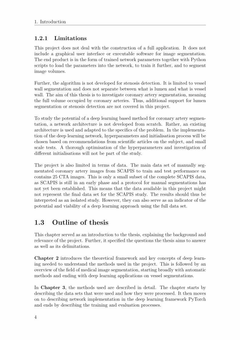
Figure 1.1: Cross section of coronary arteries in healthy vessel (left) and vessel withplaque (right). Rough outline for vessel segmentation showing full vessel (dottedgreen line), and lumen, i.e. the available space for blood flow (blue line).
With images being in 3D it is hard to view the data properly on a computer screen,adding another obstacle to the process. Even though manual segmentations are con-sidered the gold standard, an automatic method, such as Medis QAngioCT Re [3],is typically used to create a proposal segmentation. That base segmentation is thenmanually corrected by medical professionals. This procedure drastically reduces thetime needed to create the segmentations. Having fast and reliable segmentationsoftware that performs in line with what medical professionals desire is thus highlyvaluable for large scale studies such as SCAPIS. Construction of an automatic coro-nary artery segmentation tool is a complex task, partly due to vessel segmentationbeing complex in its own right, and partly due to the volumes containing a largenumber of lung vessels which should not be included in the segmentation.
With the field of image analysis moving towards deep learning approaches for seg-mentation tasks, it is natural to wonder how a deep learning algorithm would com-pare to non-learning based software like QAngioCT Re at the task of coronary arterysegmentation. If a deep learning tool performs well on the task, it could provideprofessionals with better tools in their complex task of combating terrible diseases.Deep learning algorithms have been successful on similar tasks in the past. In 2015,Ronneberger et al. introduced U-Net, a fully convolutional network for biomedicalimage segmentation which surpassed the performance of all competition on the ISBIchallenge on neuronal segmentation [4]. Further, Merkow et al. built on the generalstructure of U-Net with integration of deep supervision in their network, I2I-3D,which was used in vessel wall boundary segmentation [5]. These networks, and theirunderlying building blocks, are reviewed in more detail in Chapter 2.
Investigating the possibility of using deep learning tools for coronary artery segmen-tation is the focus of this thesis. A state-of-the-art deep learning network for medicalimage vessel segmentation is applied to the task of coronary artery segmentation,with data provided by the SCAPIS study, to determine if such an approach couldbe viable.
2

1. Introduction
1.2 Project description
The foundation for this thesis is a collaboration between researchers from ChalmersUniversity of Technology and the SCAPIS study. The Computer Vision and MedicalImage Analysis group at the Department of Electrical Engineering at Chalmers Uni-versity of Technology have gotten access to manually segmented CTA data from thestudy. The vision is to create a deep learning based tool for segmentation of coro-nary arteries as well as detection and classification of stenosis and vascular plaque.This master thesis project comprises the first step of the creation of such a tool;deep learning based coronary artery segmentation. More specifically, the questionthat this thesis aims to answer is:
Is deep learning viable for coronary artery segmentation?To answer this question, a deep learning architecture suitable for the characteristicsof this particular problem has to be chosen. The architecture needs to be able tohandle 3D image data and learn to segment tiny structures from a relatively limiteddata set. How viable the approach is can then be determined by comparison toother methods, both automatic and manual. The main research question can thusbe divided into two sub-questions:
(1) What is state-of-the-art in the field of deep learning based medical imagesegmentation in general and, more specifically, with focus on vessels?
Answering this question requires knowledge of the field; of what is being used and re-searched in medical image segmentation, and what has led the field there. Throughthis investigation, knowledge is gained both of the key elements behind deep learn-ing and the specific characteristics of deep learning applications on medical images.An exploration of the field also provides a scientific context in which to place thereport as well as ensures that the choice of network architecture can be made basedon previous research.
(2) How does a deep learning approach compare to other automatic approaches aswell as manual segmentations?
With this question, a shift from the theoretical possibilities towards practical im-plementation is made. Having acquired both a solid foundation of knowledge ondeep learning medical image segmentation and a network structure, the potential ofthe method needs to be tested. This requires reference points for performance. Asthe algorithm aims to produce segmentations as close to manual segmentations aspossible, it is natural to compare the network segmentations to those from medicalprofessionals. Further, a comparison with an automatic software that is currentlyin use for the task of coronary artery segmentation will be a clear test of its viability.
Combined, these questions lead to theoretical and practical knowledge of deep learn-ing for medical image segmentation and, specifically, a conclusion of the viability ofusing deep learning to segment coronary arteries in cardiac CTA.
3
1. Introduction
1.2.1 LimitationsThis project does not deal with the construction of a full application. It does notinclude a graphical user interface or executable software for image segmentation.The end product is in the form of trained network parameters together with Pythonscripts to load the parameters into the network, to train it further, and to segmentimage volumes.
Further, the algorithm is not developed for stenosis detection. It is limited to vesselwall segmentation and does not separate between what is lumen and what is vesselwall. The aim of this thesis is to investigate coronary artery segmentation, meaningthe full volume occupied by coronary arteries. Thus, additional support for lumensegmentation or stenosis detection are not covered in this project.
To study the potential of a deep learning based method for coronary artery segmen-tation, a network architecture is not developed from scratch. Rather, an existingarchitecture is used and adapted to the specifics of the problem. In the implementa-tion of the deep learning network, hyperparameters and initialisation process will bechosen based on recommendations from scientific articles on the subject, and smallscale tests. A thorough optimisation of the hyperparameters and investigation ofdifferent initialisations will not be part of the study.
The project is also limited in terms of data. The main data set of manually seg-mentated coronary artery images from SCAPIS to train and test performance oncontains 25 CTA images. This is only a small subset of the complete SCAPIS data,as SCAPIS is still in an early phase and a protocol for manual segmentations hasnot yet been established. This means that the data available in this project mightnot represent the final data set for the SCAPIS study. The results should thus beinterpreted as an isolated study. However, they can also serve as an indicator of thepotential and viability of a deep learning approach using the full data set.
1.3 Outline of thesisThis chapter served as an introduction to the thesis, explaining the background andrelevance of the project. Further, it specified the questions the thesis aims to answeras well as its delimitations.
Chapter 2 introduces the theoretical framework and key concepts of deep learn-ing needed to understand the methods used in the project. This is followed by anoverview of the field of medical image segmentation, starting broadly with automaticmethods and ending with deep learning applications on vessel segmentations.
In Chapter 3, the methods used are described in detail. The chapter starts bydescribing the data sets that were used and how they were processed. It then moveson to describing network implementation in the deep learning framework PyTorchand ends by describing the training and evaluation processes.
4

1. Introduction
In the following chapters, Chapters 4 and 5, the results of the implementation ofthe deep learning algorithm are presented and analysed, respectively. In these chap-ters, the focus lies on comparing the network segmentations to the Medis QAngioCTRe segmentations and the manual segmentations in order to establish the viabilityof the proposed method. Finally, a conclusion follows in Chapter 6.
5

1. Introduction
6

2Theory
This chapter aims to give the reader the foundation needed to understand the con-tents of this report, as well as to describe the research surrounding the topic. Itis sectioned into two parts; a section on deep learning and a section highlightingrelated work.
2.1 Deep learningThe need for software able to make informed decisions from large amounts of datais ever increasing in our digital society. Such software is highly dependent on theinterpretation of the data, which is a complex task to manage. Instead of manuallyprogramming the interpretation into the software, there might be benefits to gainfrom creating software that can take care of both the interpretation and the deci-sion making. Such software, able to learn how to interpret data on their own aregenerally classified as machine learning algorithms.
More generally, machine learning refers to a family of data-driven algorithms thatare able to automatically learn function mappings to desired output responses fromgiven inputs. Machine learning can be divided into two categories; supervised learn-ing where the desired output is explicitly stated, and unsupervised learning wherethe algorithm has to learn a suitable output on its own. The former will be thefocus of this report.
The actual learning process is mathematically guided and allows the algorithm tofind important features and disregard redundant information in the data without ex-plicitly being programmed to. The algorithms find new ways of representing data tofit a desired response over many iterations of tuning their parameters, usually calledtraining. This iterative optimisation process of tuning the parameters to the datacan be computationally intensive. Machine learning techniques have been aroundfor decades, but only with modern advances in computational power have their truepotential fully been demonstrated.
This section will introduce deep learning; a machine learning sub-type based onartificial neural networks. The section will explore key concepts with a specific focuson convolutional neural networks. The reader is assumed to have basic knowledge ofneural networks and machine learning. The following should serve as an overview,rather than a complete mathematical derivation of the underlying theory. For a
7

2. Theory
deeper review of deep learning, see Deep learning by LeCun et al. [6].
2.1.1 Artificial neural networksArtificial neural networks (ANNs) are a branch within machine learning, inspiredby the structure of the brain. ANNs are networks of inter-connected simple com-puting units called neurons. Just like in the brain, these neurons are responsible forpassing along information in the huge network of neurons that constitute the brain.A typical ANN structure can be seen in Figure 2.1. This type of network is knownas a feed-forward network as information only moves in one direction to produce anoutput. It is also a fully connected network due to every neuron being connectedto all neurons in the previous and the next layer. The networks usually consistsof multiple layers of neurons. The information flows through the network layer bylayer and is manipulated in each pass between layers through weighted connections,represented by arrows in the figure, and activation functions. The more layers anetwork has, the deeper it is said to be and the more complex functions it can learnto model. In the case of the network shown in Figure 2.1 there is only one hiddenlayer, resulting in a quite shallow network.
Input #1
Input #2
Input #3
Input #4
Output
Hiddenlayer
Inputlayer
Outputlayer
Figure 2.1: A simple feed-forward neural network structure with one hidden layer,mapping from R4 to R1. Neurons are represented by coloured circles.
The mathematics driving the neurons of the network is simple. Each of the neu-rons weighted inputs gets summed together, subtracted by a bias term and passedthrough an activation function before moving on to the next layer. For neuron i inthe input layer of Figure 2.1 the computation at the neuron is simply
O(I)i = a(w(I)
i Ii −B(I)i ) (2.1)
where Ii is input #i, w(I)i is the weight from the weighted connection to the neuron,
B(I)i is the bias term, a(·) is the activation function, and O(I)
i is the output from theneuron, with superscript (I) referring to the Input layer. There is no summation inthis expression due to there only being one input to this neuron. Similarly for the
8

2. Theory
jth neuron of the Hidden layer, which will be referred to with superscript (H), theexpression for the computation at the neuron becomes
O(H)j = a(
4∑i=1
w(H)ji O
(I)i −B
(H)j ). (2.2)
This expression shows the summation of the previous layers weighted outputs, butis otherwise the exact same calculation as in the previous layer. This calculationdrives all of the neurons in the network and can be seen in the Output layer, withsuperscript (O), as well,
O(O) = a(5∑j=1
w(O)j O
(H)j −B(O)). (2.3)
The propagation of information through the network, from input to output, is com-pletely described by these calculations. However, for the network to output a desiredresponse from an input it needs to learn appropriate values for its parameters, theweights w and the biases B. This is achieved through iterative updates based on aprocess named backpropagation.
2.1.1.1 Backpropagation
A simple way of describing the mathematics behind learning is that it should up-date the parameters of the network in the way that most makes the output fromthe network resemble the desired output. To do this, one first needs to describehow different from the desired output the network output is. That is the role of theloss function. There are many different viable loss functions, one of them being thesquared distance function, L = (O(O) −O∗)2 where O(O) is the network output andO∗ is the desired output, which will be used in this demonstration. The task is nowto minimise L. The ideal outcome is to reach a case of L = 0, meaning that thereis no difference between the network output and the desired output.
Assume that for a specific time tn, the weights of the network w(tn) are such thatL 6= 0, with bold w referring to all the weights stacked in a vector. One way tominimise L is to update the weights in the direction where L decreases fastest, orin other words, where the slope of L(w) is largest. Mathematically, that can becomputed by differentiation, or the gradient in the multivariate case. The updaterule for each one of the weights, based on this approach, is shown in Equation 2.4,
wj(tn+1) = wj(tn)− η ∂L∂wj
∣∣∣∣t=tn
. (2.4)
The factor η is called the learning rate and is a hyperparameter determining howlarge a single update step should be. The minus sign ensures that the update isdown the slope, so that L decreases. This method of updating the weights is appro-priately named gradient descent, and is one of multiple viable optimisation methods
9

2. Theory
to tune the weights of a neural network.
Calculating ∂L∂wj
∣∣∣t=tn
is a straight forward task through the use of the chain rule. Theterm can be split into its constituents as shown in Equation system 2.5, exemplifiedfor the small neural network described in Figure 2.1 and Equations 2.1-2.3, wherethe gradient is calculated for a weight connecting the hidden and the output layer,w
(O)j , a weight connecting the first layer and the hidden layer, w(H)
ji , and a weightconnecting the input to the first layer, w(I)
j :
∂L
∂w(O)j
= ∂L
∂O(O)∂O(O)
∂w(O)j
= 2(O(O) −O∗) a′︸ ︷︷ ︸=δ(O)
O(H)j = δ(O)O
(H)j
∂L
∂w(H)ji
= ∂L
∂O(O)∂O(O)
∂O(H)j
∂O(H)j
∂w(H)ji
= δ(O) w(O)j a′︸ ︷︷ ︸
=δ(H)j
O(I)i = δ(O)δ
(H)j O
(I)i (2.5)
∂L
∂w(I)i
= ∂L
∂O(O)∂O(O)
∂O(H)j
∂O(H)j
∂O(I)i
∂O(I)i
∂w(I)i
= δ(O)δ(H)j w
(H)ji a′Ii.
The same procedure is done for all of the weights and biases of the network. Theright hand side expressions in Equation 2.5 are easy to evaluate at the specific timetn once the values have been propagated through the network. As can be seen fromthe δs, the gradients all build on each other just like Equations 2.1-2.3 leading tothe network output, but in the opposite direction. The input data flows through thenetwork from input layer to output layer in order to calculate the output and thefirst gradient. The updates are then calculated from the output layer to the inputlayer, as gradients are propagated backwards in the network. This is the process ofbackpropagation, first introduced by Rumelhart et al. in 1986 [7].
2.1.1.2 Activation function
While present in all layers of the network in Figure 2.1, the role of the activationfunction has yet to be described. To understand why it is needed, assume a networkwithout activation functions. In vector notation, the computation at every layerof the network can be described as follows: f(x) = a(Ax + B), where a(·) is theactivation function, x ∈ Rn is the input to the layer, A ∈ Rm×n is the weight matrix,and B ∈ Rm is the bias vector. It is then clear that in a network without activationfunctions, every layer represents an affine mapping: Ax+B. Assume two such layers,with affine mappings f(x) = Ax + B and g(x) = Cx + D. Propagating x throughboth layers, first through g and then through f , results in f(g(x)). Expanding thisexpression gives as follows:
f(g(x)) = A(Cx +D) +B = (AC)x + (AD +B),with (AC) being a matrix and (AD + B) being a vector, the result is a new affinemapping. Thus; combining affine mappings gives no new complexity to the model.
10
2. Theory
Multiple layers would not have any benefits in a neural network, since they couldalways be represented by a single layer. However, with the addition of non-linearactivation functions between the affine mappings the linearity is broken and thenetwork can model much more complex mappings.
While there are countless non-linear functions, many neural networks use one ofReLU(x) = max(0, x), tanh(x) or the sigmoid function; σ(x) = 1
ex+1 . The reasoningbehind this is that these functions have gradients that are easy to compute, whichis crucial for learning as shown in Section 2.1.1.1.
2.1.1.3 Overfitting
The training of a neural network may seem straight forward but the process is quitedelicate and complex. There are unwanted phenomenons that need to be consid-ered, such as overfitting. Overfitting is the phenomenon where the neural network isovertrained on the training data set to the point that it fails to properly process newdata. While producing correct results on the training set, it might have been tunedtoo well to the specific samples of the training set, rather than learning techniquesto properly process it. That way, it becomes more of a dictionary of the trainingdata, giving the correct output for the chosen input, but not being able to handlenew data. This behaviour is very undesirable and there are ways to combat it suchas data augmentation and drop-out layers. These methods are examples of regular-isation methods which aim to help the network learn to generalise from the data itsees in order to handle new data well.
Data augmentation refers to different methods of extending the available data throughsoftware. By doing natural manipulations on the data, more variation can be repre-sented which gives the network better conditions to learn important features. Withmore variation represented, the training process is less susceptible to overfitting.Which manipulations are viable for augmentation depends on the data. In the caseof images, typical manipulations include flipping along axis, rotation, scaling andnoise addition. For the coronary artery data, flipping along axis is not a viablemanipulation due to the asymmetry in the vessel structure. The left and right - aswell as top and bottom, and front and back - sides have characteristic shapes andflipping will not represent naturally occurring data. Small rotations, scaling, andadditive noise are on the other hand feasible and were implemented in this project.
Drop-out is another technique to combat overfitting by randomly dropping unitsand their connections in each training iteration [8]. Dropping refers to removing theunits from the learning process. This ensures that the network is not too dependenton any single unit or small group of units. The network constantly has to learn toprocess the data correctly from a new set of active neurons each training iteration,which has been shown to significantly reduce overfitting.
Another regularisation method is weight decay, which reduces the size of the weightsby a factor every weight update. This has been shown to attenuate irrelevant com-ponents of the vector, improving the networks ability to generalise from data [9].
11
2. Theory
2.1.1.4 Optimiser
There are different ways of updating the network parameters, or optimising them,based on the gradients. Gradient descent, as mentioned in Section 2.1.1.1, is onesuch optimiser. In reality, stochastic gradient descent (SGD) is used in favour ofregular gradient descent, due to it being faster and computationally cheaper. Gra-dient descent requires the gradients to be calculated for the entire training data setfor each update. SGD allows for updates after every data sample, which is muchmore efficient.
While reliable, SGD requires careful choice of hyperparameters to tune the algo-rithm. An optimal learning rate with or without decay, weight decay factor and amomentum factor have to be set manually and greatly affect the outcome of theoptimisation. Both learning rate and weight decay have been explained previously.Momentum acts as a sort of memory in the training process. Instead of calculatingcompletely new update terms every iteration, the new update term is complementedby the previous update term, typically scaled down by a factor. The scaling factorthen tunes the balance between previous update terms (the memory) and the cur-rent update term.
Another optimiser, Adam, builds on SGD and is able to adjust learning rate on itsown and individually for each weight [10]. For specific details of how this is achievedthe reader is referred to the paper in which the method is described, i.e. [10]. SGDstill sets the bar for finding good minimas of the loss function, whereas Adam mightget stuck in bad local mininas. However, Adam is faster to converge and does notrequire the same level of manual tinkering.
2.1.1.5 Loss function
The loss function solely determines what the network is optimised for, since it iswhat the learning algorithm minimises. It is a tricky task to choose the optimal lossfunction. Typically, there is a discrepancy between the qualitative characteristicswanted from the network and what can be mathematically described. An exampelof a simple loss function was demonstrated in Section 2.1.1.1; the squared distanceloss L = (O − O∗)2. There are many different loss functions used in deep learning,with each being suited for specific tasks. For image segmentation tasks with fullyconvolutional neural networks, binary cross entropy (BCE) is a commonly used lossfunction [4, 5]. It is formulated in Equation 2.6, with O = (o1, ...oN) being thenetwork output and O∗ = (o∗1, ..., o∗N) being the desired output, as described inSection 2.1.1, for an image with N voxels:
lBCE(O,O∗) = −N∑n=1
o∗n · log(on) + (1− o∗n) · log(1− on). (2.6)
This is a measure of negative log likelihood and quantifies the difference between twoprobability distributions, where the two terms in the sum represent the two classes,i.e. the binary nature. Intuitively, one can think of cross entropy as a measure ofhow easy it is to predict O∗ from O, where lBCE closer to 0 means easier.
12

2. Theory
2.1.1.6 Deep supervision
In supervised learning applications, where the desired output is explicitly stated inthe training process, the parameter updates are typically calculated based on theloss from comparing the network output and the desired output, as previously de-scribed. In theory, one could also add outputs from deeper layers in the network andcalculate losses from them as well, in order to force the network to produce viableoutputs in its earlier stages. This is the idea behind deep supervision, which wasfirst introduced by Lee et al. [11]. Their article shows that the addition of deep su-pervision not only decreases classification error rate, but also speeds up convergence.
Assume a network with N total outputs, from N different layers in the network.Deep supervision works by calculating a loss for each of the outputs. Generally, tocompare the network output to the desired output one might need an additionallayer to produce an output shape corresponding to the desired output. All of thenetworks losses are then summed together to create the total loss, which is usedfor parameter optimisation. With N levels of supervision, and the individual lossesdenoted by l, the total loss, L, is simply as shown in Equation 2.7, with superscriptdenoting level,
L =N∑n=1
l(n)(O(n),O∗). (2.7)
2.1.1.7 Transfer learning
Transfer learning refers to the act of applying gained knowledge on one task toa new task. This is largely relevant in the field of deep learning. In many deeplearning applications, there might not be a large enough data set to generalise from.Something that can help is then to initially train the network on different datasets with similar features to the main data set, before the main training. The datarepresentations learnt from those data sets might improve the learning on the maindata set, which gives the network a head start on learning to generalise [12]. Thistraining on different data sets before training on the main task, generally known aspretraining, is a common practice in deep learning applications.
2.1.2 Convolutional neural networksConvolutional neural networks (CNNs) are a special category of feed-forward net-works whose core structure was first introduced under the name Neocognitron byFukushima et al. in 1982 [13]. Since then, CNNs have become largely popular incomputer vision applications. They are especially well suited for image analysisdue to their shift invariance and non-sensitivity to natural image variations such aslighting and visual clutter [14]. As of 2017, CNN-based architectures are the topperformers in ImageNet’s Large Scale Visual Recognition Challenge in object detec-tion, object classification and object localization [15, 16].
13

2. Theory
What separates CNNs from the network type introduced in Chapter 2.1.1 is thatthe operation driving the network is filtering, performed by discrete convolutions,rather than Equations 2.1-2.3. Each layer of a convolutional neural network appliestrained filters on the input through convolutions. The filters are typically muchsmaller in size than the image, meaning that they are applied locally to the image.They are then shifted a set distance in the image, referred to as stride length, suc-cessively building up the output.1 Each output voxel is the result of a dot productbetween a filter and a local neighbourhood of the corresponding voxel in the input.A visualisation of this is shown in Figure 2.2. This local application of the samefilter all across the image is what gives CNNs their shift invariance.
Figure 2.2: Visualisation of how the output is formed in a CNN. A filter is appliedto a local neighbourhood in the image through dot product. The result is a singlevalue at the centre of the corresponding position of the neighbourhood in the outputimage. The filter is applied to the entire input image in this way.
The filtering process creates a loss of pixels around the borders, which can be seenin Figure 2.3 as the filter can’t be moved up or right in the input image fromits current position, leaving the space above and to the right of the output pixelempty. This can be handled by zero padding the input, placing zeros on the outsideof the input image, allowing the filter to be applied at the very borders of the image.
Intuitively, the filtering can be thought of as a means of feature extraction, wherethe network learns important features of the data, as well as the appropriate filtersto extract them. It then applies these filters regularly along the image, "looking"for the specific features it has been trained for. The output becomes a feature map,
1In reality, filters are duplicated to match the size of the input image in order to perform thefull filtering in one operation, rather than shifting and applying the filters iteratively.
14

2. Theory
containing information of if and where features are located. At shallow levels inthe network these features may be distinctive gradients in images or characteristicshapes of signals, but deeper layer filters are often far too abstract to have inter-pretable conceptual counterparts.
In a CNN, convolutional filters are often interlaced with activation functions andpooling layers. Pooling layers reduce the size of the input, typically by half along eachaxis. There are different ways of pooling; max pooling converts a neighbourhood ofvoxels into one voxel containing the largest value from the neighbourhood, averagepooling converts the neighbourhood into a voxel containing the average value, andso on. An example of max pooling on a 2D image with a pooling window of size(2, 2) and a stride length of 2 is shown in Figure 2.3. Pooling enables the network towork with the data in multiple scales. By pooling the input the network effectivelygets a larger receptive field. As in Figure 2.3, four pixels represent a total of 16pixels in the original image. This allows CNNs to learn features in both large andsmall scales; using both global and local image information.
Figure 2.3: Maxpooling of the image matrix on the left with a pooling windowsize of (2,2) and a stride length of 2. The result is seen on the right, where eachpixel is the maximum value of their respective neighbourhood in the image.
2.1.3 TerminologyTo provide the reader with a quick view of terms that are useful to know in relationto deep learning and the specifics of this thesis, a small dictionary is shown below.
Activation function Non linear function to break linearity in networks.Epoch One full pass over every data point in the training process.Layer Every single function applied to the input can be thought of as a layer that
the input propagates through and is changed by.Level A block within the neural network where image resolution is constant.Neuron A single computation unit in the network.Tensor A multidimensional extension of vectors and matrices.Training The process of having a neural network learn to produce desired outputs
from inputs through iterative updates of the network parameters.
15

2. Theory
Volume / 3D image Used interchangeably to refer to the CTA images, which are3D image volumes composed of stacks of 2D images.
Voxel The 3D equivalent of a pixel.
2.2 Previous work on medical image segmenta-tion
Manual image segmentation is both hard and time consuming and many automaticapproaches have been developed with the aim to reduce the amount of manual work.This section provides an overview of important automatic segmentation techniques,both non-learning and deep learning based, used in medicine and specifically forvessels.
2.2.1 Non-learning based medical image segmentationAutomatic image segmentation techniques have been used since before deep learn-ing algorithms were applied to the task. A technique that has been around sincebefore the 21st century is the use of Watershed. Watershed is an algorithm thatinterprets an image as a topological map where pixel intensities represent height[17]. Simplified, the segmentation is constructed from borders defined by ”height”differences. In 2004, Yu-Len Huang et al. successfully implemented Watershed tosegment breast tumors in 2D sonography [18]. The tool was used to assist medicalprofessionals, aiming to save time and help inexperienced physicians reach the cor-rect diagnosis.
Another automatic approach used specifically for vessel-like structures is Frangi fil-tering [19]. The filter enhances tube-like structures based on the eigenvalues ofthe Hessian matrix, locally applied to the image. The Hessian is a matrix con-taining the second order partial derivatives. From its eigenvalues one can deter-mine the local principal directions in the data, making it a good measure for lo-cal tube-likeness in an image. Among others, a method based on Frangi filteringwas applied by Martinez-Perez et al. to segment blood vessels in fluorescein reti-nal images and reached 0.94 in segmentation accuracy (in this case meaning thenumber of correctly segmented pixels divided by the total number of pixels)when compared to medical professionals [20].
A commercial software building on Frangi filters, exclusively used for coronary arterysegmentation, is the Medis QAngioCT Re software [3]. The frangi filtered outputin QAngioCT Re is post-processed using geometric information to separate coro-nary arteries from unwanted structures. To separate the aorta from the rest of thecoronary artery tree the software uses a Hough transform to determine its location.The Hough transform is a feature extraction technique excelling at the detection ofcircular shapes in images [21]. The software has performed well on the RotterdamCoronary Artery Evaluation Framework, currently placing 10th in coronary arterysegmentation and 14th in stenoses detection [22, 23]. The SCAPIS study utilises
16

2. Theory
Medis QAngioCT Re for automatic coronary artery segmentation.
Even though automatic approaches like Watershed and Frangi filtering have provenuseful, the field of image segmentation is shifting away from such non-learning basedtechniques towards deep learning. This is in part due to the impressive performanceof CNNs in image analysis.
2.2.2 Deep learning based image segmentationDue to CNNs impressive performance in image classification, as mentioned in Sec-tion 2.1.2, it was only natural to investigate their performance on segmentationtasks as well. The first approaches used pixel-by-pixel classifications, where a singlepixel was classified based on the pixel values of a square neighbourhood centeredon it. The filter is applied in a sliding-window manner, being locally applied to aneighbourhood at a time and building up the output as the filter moves across theimage. With this approach, Ciresan et al. used four stages of convolutional filterstogether with fully connected layers to produce segmentations from pixel-by-pixelclassification and outperformed the previous state of the art in the ISBI 2012 EMSegmentation Challenge [24]. Ning et al. used a similar architecture to segmentimages of C. elegans embryos into five classes with an error rate of 29.0% [25].
A breakthrough by Long et al. in 2015 with a network architecture named fullyconvolutional networks (FCNs) enabled the use of full image-to-image segmentations,rather than constructing segmentations from pixel-by-pixel classifications on imagepatches [26]. As the name suggests, FCNs have no fully connected layers. They arecomposed solely from convolutional filter layers, pooling and activation functions.This allows the networks to be size-agnostic, able to produce a full size segmentationregardless of the input image dimensions. In their paper, Long et al. show FCNsstrong ability to produce both accurate classification and localisation while workingon a full image, improving accuracy and reducing computational cost when comparedto patch-by-patch pixel classification.
2.2.3 Medical image segmentation with U-NetIn 2015, Ronneberger et al. introduced a convolutional neural network structurespecifically developed for biomedical image segmentation called U-Net, building onFCNs [4]. At its time of introduction, U-Net surpassed the performance of all othermethods on the ISBI challenge for neuronal segmentation in electron microscopy im-ages, as well as the ISBI cell tracking challenge. What makes it ideal for biomedicalimage segmentation is its ability to learn from a relatively small data set, somethingthat can otherwise be a problem in medical applications.
The U-Net network structure is shown in Figure 2.4. It has the typical CNN compo-nents of filters, activation functions which are ReLU in this case, and pooling. Whatseparates it from other architectures is that after the standard encoder structure (leftside) of moving down in resolution and extracting features, it has a decoder structure
17

2. Theory
(right side), turning the features into a full resolution segmentation in the same levelstructure as in the encoder. This gives the network a U-shape, explaining the originof its name. The upscaling in the decoder is performed by what Ronneberger etal. call up-convolutions, also known as transposed convolutions or deconvolutions.There are also interconnections between the levels of the encoder and the decoder.The outputs from the encoder levels are concatenated to the corresponding decoderlevel inputs, where they are mixed together by convolution. As the network poolsthe data in the encoder, the shallow fine detail information gets lost with the im-age size reduction. This is a problem, since small scale localisation is important inmedical images. Having the encoder responses added back into the decoder combatsthis problem, allowing the final layers of the network to have information of boththe shallow fine detail localisation and deep semantic information determining whatclass the individual pixels belong to.
Figure 2.4: Image describing U-Net from the original paper by Ronneberger etal. [4]. The filter sizes are written on top of every convolutional layer and the filterinput sizes are written on the sides.
The U-net structure has also been extended to 3D image segmentation by Çiçek etal. [27]. One might assume that 3D data could be sliced into a stack of 2D imagesand segmented slice by slice before restructuring the segmentations into a 3D vol-ume, making the need for a 3D version of U-Net unnecessary. However, anatomicalstructures have features in all three spatial dimensions, meaning that leaving outone dimension would limit the information available to the network. Slicing 3D datais thus not good practice when working with medical images, unless other measuresare taken to account for the three-dimensionality of anatomical features.
2.2.4 Vessel wall segmentation with I2I-3DIn 2016, Merkow et al. introduced a network structure originally designed for vesselwall segmentation named I2I-3D [5]. The architecture builds on a 3D U-Net struc-
18

2. Theory
ture with the addition of deep supervision. It has the general structure of a fine tocoarse, or shallow to deep, encoder followed by a coarse to fine, or deep to shal-low, decoder with four levels, as well as the interconnections between encoder anddecoder that are present in U-Net. The complete structure, together with specifica-tions of the number of filters used is shown in Figure 2.5. Upsampling is performedby deconvolutions. The filter levels contain no drop-out layers and are completelymade up of the convolutional filters and ReLU functions shown in the image. Themixing layers in the decoder, coloured orange, combine the information from theprevious layer with the corresponding encoder level output through 1 × 1 × 1 con-volution filters. Merkow et al. showed that this approach, with deep supervisionplaced at the end of every decoder level as illustrated in Figure 2.5, outperformedthe previous state of art in 3D vascular boundary detection.
Figure 2.5: Image of I2I-3D network structure from Dense Volume-to-VolumeVascular Boundary Detection by Merkow et al. [5]. The filter size is written to theleft of every filter layer. Deep supervision is applied at the end of every decoderlevel.
With I2I-3D having proved itself in vessel wall boundary detection, it was a naturalchoice to investigate its coronary artery segmentation potential. The development ofa segmentation tool in this thesis was thus centered around this network architecture.
19

2. Theory
20

3Data and Methods
This chapter will describe the data sets used in the project and how they wereprocessed and used to train the model. The deep learning framework and the net-work implementation will also be described, as well as the training and evaluationprocesses.
3.1 Data
As described in Section 2.1, the data is what drives the training in deep learning andis thus extremely important. The network needs to generalise from the informationit sees, meaning that the quality of the data can make or break the application.A common approach in deep learning is to preprocess the data before feeding it tothe network, and to pretrain the network on different data sets before training onthe main task. Even if the pretraining data sets are different to the main data set,they allow the network to start learning features, as described in Section 2.1.1.7.To virtually enlarge the data set it is also good practice to augment the data. Thischapter serves to introduce the data sets, as well as the preprocessing and augmen-tation methods used.
Four data sets were used to train the network; three data sets for pretraining inaddition to the main data set of manually segmented coronary arteries. All data setswere produced by CT scans, ensuring that the network does not encounter the extradifficulty of learning to handle images produced by different imaging modalities.
3.1.1 VISCERAL (VS) data set
A subset of the data from the study Cloud-based evaluation of anatomical structuresegmentation and landmark detection algorithms: VISCERAL anatomy benchmarkswas used for pretraining, here referred to as data set VS [28]. The study containsboth MR and CT data with multiple segmented anatomical regions in the body,e.g. the sternum, the pancreas and the spleen. A subset of 20 CT volumes ofthe sternum were used in pretraining, due to their similarity in composition to thecoronary artery images as they are images of the same anatomical region. Thesevolumes had voxel dimensions of 0.82 × 0.82 × 1.5 mm3 An example image fromthe set is shown in Figure 3.1. The data set was split into two sets; a training set(17/20) and a validation set to evaluate the training (3/20).
21
3. Data and Methods
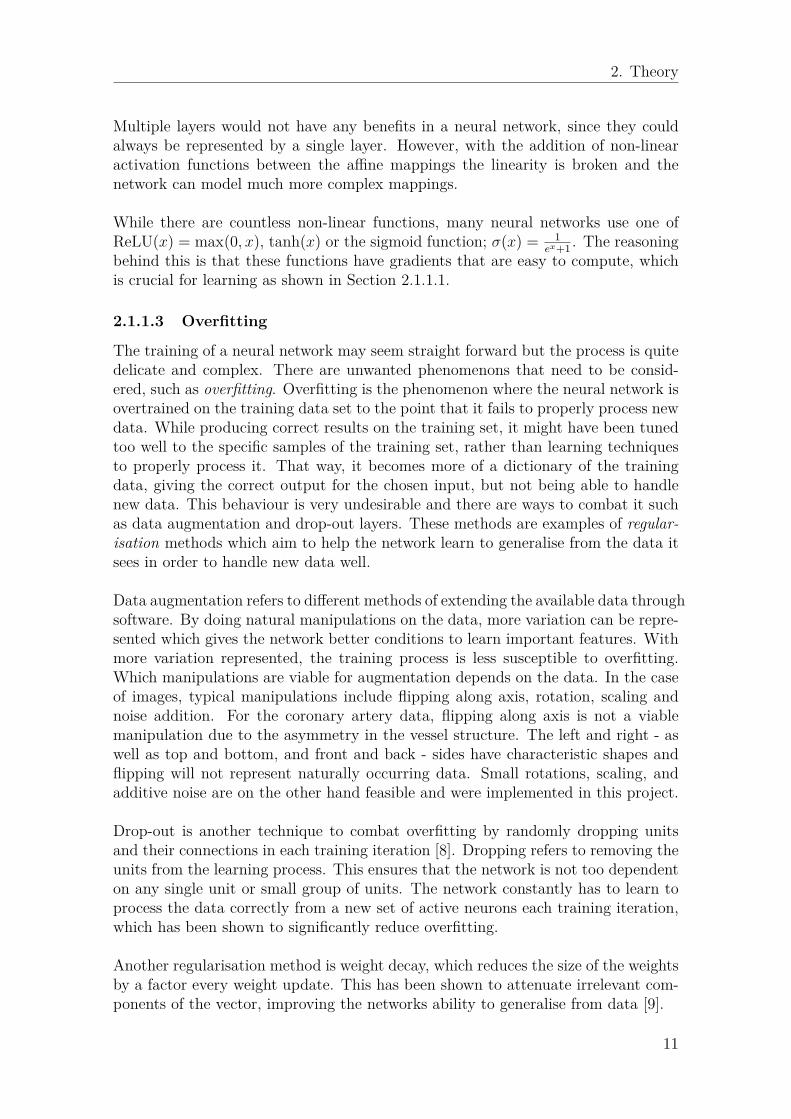
Figure 3.1: Example image volume from the VS data set, sliced along the threespatial axes. The corresponding segmentation of the sternum is marked in red.
3.1.2 SCAPIS pericardium (PS) data set
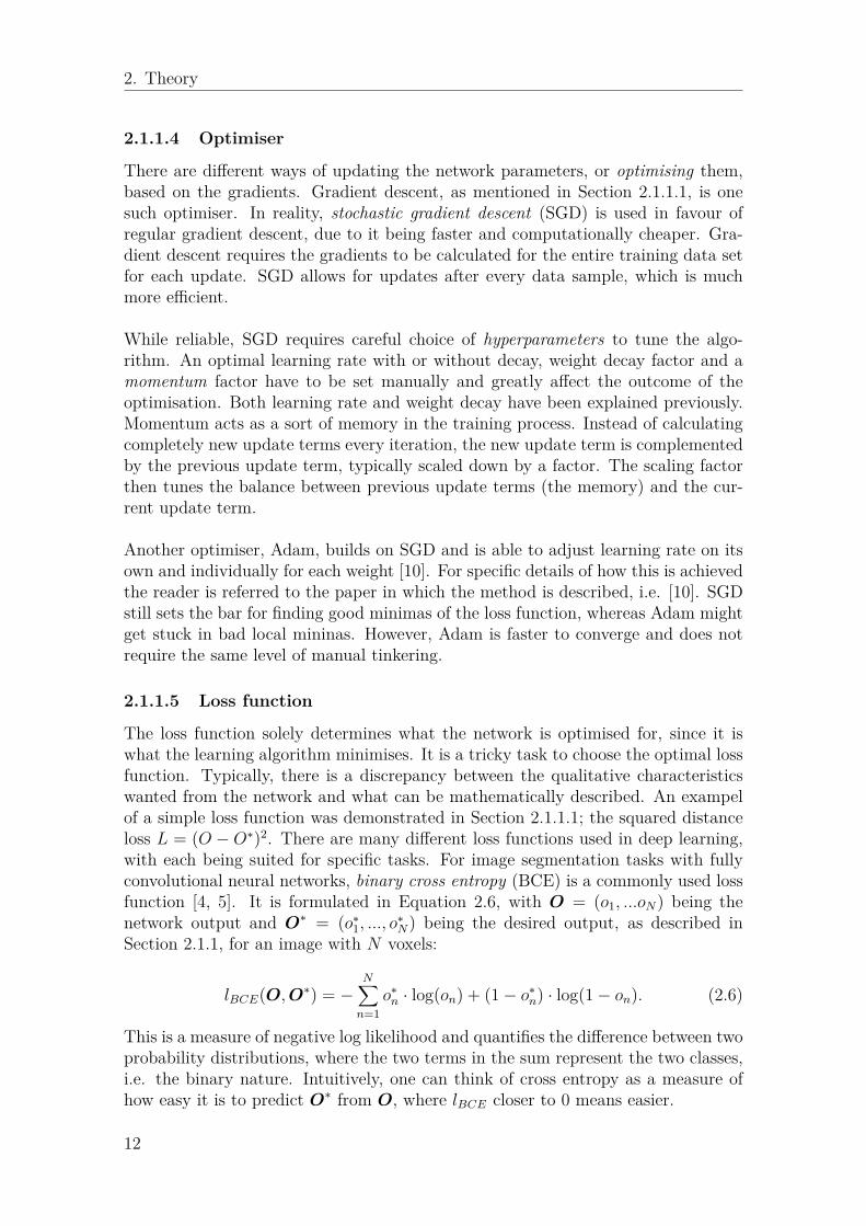
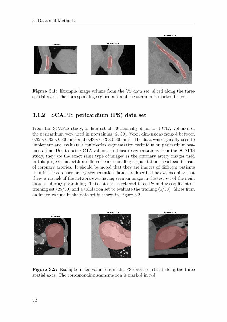
From the SCAPIS study, a data set of 30 manually delineated CTA volumes ofthe pericardium were used in pretraining [2, 29]. Voxel dimensions ranged between0.32×0.32×0.30 mm3 and 0.43×0.43×0.30 mm3. The data was originally used toimplement and evaluate a multi-atlas segmentation technique on pericardium seg-mentation. Due to being CTA volumes and heart segmentations from the SCAPISstudy, they are the exact same type of images as the coronary artery images usedin this project, but with a different corresponding segmentation; heart sac insteadof coronary arteries. It should be noted that they are images of different patientsthan in the coronary artery segmentation data sets described below, meaning thatthere is no risk of the network ever having seen an image in the test set of the maindata set during pretraining. This data set is referred to as PS and was split into atraining set (25/30) and a validation set to evaluate the training (5/30). Slices froman image volume in the data set is shown in Figure 3.2.
Figure 3.2: Example image volume from the PS data set, sliced along the threespatial axes. The corresponding segmentation is marked in red.
22

3. Data and Methods
3.1.3 Medis automatic coronary artery segmentations (AS)data set
Automatically produced coronary artery segmentations from the software MedisQAngioCT Re working on the SCAPIS data were also used in pretraining, referred toas the AS data set [2, 3]. The data was of two different voxel sizes; 0.332×0.332×0.5mm3 and 0.32×0.32×0.30 mm3. Medis QAngioCT Re segments all coronary arteriesit can find, regardless of size. This means that small, clinically irrelevant vessels willbe part of this data. The data set contains 77 CTA volumes with segmentationswhich have not been reviewed by medical professionals. Althogh not manuallycorrected, AS contains acceptable segmentations of the coronary artery tree for thetask of helping the network learn to segment vessel like structures in pretraining.The classes are highly imbalanced in this data set, with coronary arteries making uponly an average of around 0.1% of the image voxels. This imbalance can be seen inthe example image in Figure 3.3. The data was split into three sets: a training setused for training (59/77), a validation set used to evaluate the performance in thetraining process (11/77), and a test set which was only used once during the finalevaluation (7/77).
Figure 3.3: Example image volume from the AS data set, sliced along the threespatial axes. The corresponding segmentation is marked in red.
3.1.4 Manual coronary artery segmentations (MS) data setThe main data set for this study consists of 25 manually corrected segmentationsfrom the Medis QAngioCT Re software performed on SCAPIS data. These manualcorrections typically consist of small scale corrections of placing segmentation bor-ders, as well as removal of small vessels far out in the coronary artery tree. Vesselswith a diameter less than 2 mm are typically deemed clinically irrelevant and re-moved from the segmentation. Naturally, these images are similar to the AS dataset, as can be seen in Figure 3.4. These volumes had the same voxel sizes as the ASdata; (0.332, 0.332, 0.5) mm and (0.39, 0.39, 0.5) mm.
23

3. Data and Methods
Figure 3.4: Example image volume from the AS data set, sliced along the threespatial axes. The corresponding segmentation is marked in red.
Each of the 25 CTA volumes were processed by two medical professionals, A andB, resulting in two sets of segmentations: MS-A and MS-B. The network trainedon both MS-A and MS-B. The data was split into 3 sets: a training set (18/25), avalidation set (4/25), and a test set for the final evaluation (3/25). Just like the ASdata set, this data set also has a class imbalance with around 0.1% the image voxelsbeing coronary arteries.
One should note that since medical professionals decide what vessels are interestingenough to be part of the segmentation, there is subjectivity involved in the manualcorrections. As such, there is no guarantee that two medical professionals producecompletely similar segmentations from the same image data. Over the 25 images,the mean Dice index similarity was 0.81 and the mean modified Hausdorff distancesimilarity was 2.34 between MS-A and MS-B.
3.1.5 PreprocessingAll data samples were normalised to have zero mean and unit variance. A largerange of values in data will create a large range of values in the features extractedfrom the filtering processes in the network. Normalising all data to zero mean andunit variance is a way to keep the data consistent. In Efficient Backprop, LeCun etal. describe that this process facilitates faster convergence [30].
Due to CT images having different sample spacings in different spatial directions,the images are scaled to cube voxels. Having cube voxels means that moving onevoxel in any direction represents the same real world distance travelled, no matterwhich direction is chosen, so that the image matrix represents the real world moreclosely. The information needed for this, the slice thickness (z-dimension) and thepixel spacing (x-y-dimensions) from the CT scan, is readily available in the DICOMheader incorporated into every DICOM image file [31].
24

3. Data and Methods
The VS data set images were small enough to be processed on the available GPUmemory, being of size 176, 176, 128. The PS data set was however too large and wastherefore downscaled to a factor 0.39, to a size of (200, 200, 176). For the AS andMS data sets, the original image size of (512, 512, Z), where Z represents a variablenumber of slices, also proved too large to process. This meant that all images wereshrunk to a maximum size of (248, 248, Z), where Z had a maximum value of 184due to the GPU memory restriction. Any value larger than 184 in the z-dimensionresulted in a cut down to 184, equally from the top and bottom of the image. Theimage shrinking was achieved through downscaling to a factor of 0.5 followed bythe removal of a 4 voxel wide frame in the x and y dimensions. No coronary arteryvessels are present in this 4 voxel wide frame, so this removal should not affect theperformance of the network.
3.1.6 Overview of data fed to networkTo summarise; the network was fed data from four different data sets. Two of whichare of the anatomical region surrounding the heart, but not of coronary arterysegmentations, VS and PS, and two coronary artery segmentation data sets, ASand MS, created by an automatic software and manually by medical experts, re-spectively. All of the data was normalised to zero mean and unit variance and, ifneeded, shrunken down to a smaller size due to GPU memory limitations.
During training, full images were used for the VS and PS data sets, and both fullimages and patches from the images were used for the AS and MS data sets, withroughly 1/6 of the images used in full size and 5/6 used to create patches. Dataaugmentation was performed both on the full images and on the patches for the twolatter data sets in order to prevent overfitting.
3.1.7 Data AugmentationData augmentation was performed online, meaning that it was done in the trainingloop. Offline data augmentation refers to augmentation done separately from train-ing where the manipulated images are stored as an extra data set. With 3D imagesbeing quite large to begin with, this can become a problem. Another drawback isthat the network will see the same images every epoch. The network may still besusceptible to overfitting because of this. With online augmentation, the data setis instead loaded into the training loop where it is manipulated with the methodsdescribed in Section 2.1.1.3 every iteration. Since angles of rotation, scales, andnoise are chosen randomly, new transformations of the images will be used everyepoch, ensuring that the network never sees the same image twice.
The transformations used on the data were small scalings, small rotations and addi-tive noise. Implementation of noise and rotations are straight forward with PythonsSciPy library [32]. numpy.rand.normal() was used to generate both noise (mean 0,variance 3 · 10−2) and small rotation angles (mean 0, variance 1), and the rotationswere performed using scipy.ndimage.interpolation.rotate(). On the patches,
25

3. Data and Methods
scaling was implemented by selecting different sized patches from the image. With32 × 32 × 32 acting as the standard patch size, a side length was chosen from anormal distribution with a mean of 32 and a variance of 3.2, with lower and upperlimits set to 16 and 64 respectively. On the recommendation of Merkow et. al, onlypatches with at least 0.25% coronary artery voxels were used in training [5].
3.2 Implementation of I2I-3DThe focus of this thesis lies on the I2I-3D network described in Section 2.2.4. Thissection describes the implementation of I2I-3D in the deep learning frameworkPyTorch. A detailed description of the training process is included, with choicesfor initialisation, loss function, and optimiser.
3.2.1 PyTorchPyTorch is a deep learning framework released on Jan 19 2017 [33]. At the timeof writing this report, PyTorch is still in early-release beta but has already beenadopted by the deep learning research community. A year after its beta release onJan 12 2018, monthly arxiv.org framework mentions where 72 for PyTorch, com-pared to 273 for the widely popular TensorFlow, 100 for Keras, 94 for Caffe, and 53for Theano, showing its quick rise in popularity [33].
PyTorch was created for deep Python integration and builds upon the scientificcomputation package Torch for Lua [34]. Unlike frameworks like Tensorflow whichrequire the user to create a static graph of the network which is differentiated sym-bolically before any information is passed to it, PyTorch simply runs computationsfunction by function, line by line, and dynamically constructs the network graphwith each new computation. Although requiring that differentiation is performedevery iteration, it offers the possibility to easily integrate new code into the graphand change the network structure dynamically and without compilation [35]. Anadditional benefit when debugging is that one only has to break through the Pythonabstractions, rather than both the Python abstractions and the abstractions of astatic graph to find errors.
PyTorch supports NVIDIAs parallel computing platform, CUDA, for GPU process-ing. Loading networks and PyTorch tensors containing the inputs and outputs to aGPU is handled by the cuda() function available in all tensor and neural networkobjects. Using multiple GPUs for data parallelisation is initiated by passing theneural network model through the torch.nn.DataParallell() function. Both ofthese computation accelerators were used in training and evaluation.
3.2.2 Implementation of I2I-3D architectureThe I2I-3D network was implemented from scratch in PyTorch based on the articleby Merkow et al. and their Caffe implementation available at GitHub [5, 36]. In
26

3. Data and Methods
PyTorch, all neural networks are subclasses of the torch.nn.Module class. Thisclass contains all the functions needed to build a network; fully connected layers,convolutional layers, activation functions, pooling layers, and so on. PyTorch alsohas a sequential container, torch.nn.Sequential, which builds a block of the neu-ral network from multiple functions connected in the order they are added to thesequential container. For example, the line of code below will create a neural net-work block consisting of two layers of (5, 5) convolution filters acting on a singlelayer input, followed by a ReLU activation function.
torch.nn.Sequential(torch.nn.Conv2d(1, 2, (5,5)), torch.nn.ReLU())
The sequential block was used to build each level in the encoder and the decoderof the I2I-3D network. A snippet of the code, containing the class construction andthe first level of the encoder is shown below.
import torch
import torch.nn as nn
class I2I3D(nn.Module):
def __init__(self):
super(I2I3D, self).__init__()
self.encoder_lvl_1 = nn.Sequential(
nn.Conv3d(1, 4, (3,3,3), padding=1),
nn.ReLU(),
nn.Conv3d(4, 4, (3,3,3), padding=1),
nn.ReLU()
)
The code shows the creation of the I2I3D class, as well as the construction of thefirst encoder level, with two sets of four filter layers using filters of size (3, 3, 3) withzero padding to keep the dimensions unaltered, each followed by ReLU activationfunctions. The structure of the network is specified in the __init__ function, mean-ing that it is created whenever an instance of the I2I3D class is created. The flowof information has to be specified in a function named forward within the class,showing how the network output is formed from the input, using the created blocksfrom __init__. For example, if the I2I3D class only had the one layer shown above,the forward function might look like the following:
def forward(self, x):
output = self.encoder_lvl_1(x)
return output
The encoder and decoder blocks, as well as the mixing layers for interconnectionsand upscaling layers for deep supervision outputs were created in the __init__()function and connected in the forward() function. To create probabilistic out-puts, where each voxel has a probability of being a coronary artery, representing thenetwork’s certainty in its classification, a sigmoid was added to the outputs. Thisnormalises the voxel values to the interval (0, 1) which is easily interpreted. A voxel
27

3. Data and Methods
value larger than 0.5 was determined as coronary artery in the binarisation processto create a segmentation.
One change to the original network architecture is the filter sizes used in the net-work. Merkow et al. suggest using 32, 128, 256 and 512 filter layers in the fourlevels. Due to memory limitations of the GPUs, these were changed to 4, 8, 16, and32 layers, which represents a significantly lower amount of network parameters. Oneattempt to tackle memory limitations was done by converting parameters and datato floating point 16 instead of floating point 32 during training through a methodknown as mixed precision training. Unfortunately, this attempt was ultimately un-successful. For more information on mixed precision training the reader is referredto an article by NVIDIA [37].
In total, the implemented version of I2I-3D network consists of 49 layers, countingconvolution and ReLU layers separately and including the 3 upscaling and/or flat-tening layers, and a total of 113,185 trainable parameters. A schematic illustrationof the network structure is shown in Figure 3.5, where filter sizes are written onthe side of every filter layer. The flattening layers are used for the deep supervisionoutputs to create single-layered outputs from the 8 and 16 layered decoder outputs.The full code for the network can be found on GitHub1.
Figure 3.5: The I2I-3D network archtitecture implemented in PyTorch for coronaryartery segmentation.
1https://github.com/frefdrk/i2i3d-pytorch
28

3. Data and Methods
3.2.3 Training I2I-3DMoving from just a network structure to a useful model requires training. A trainingloop in PyTorch requires the specification of a loss function and an optimiser. Choiceof loss function, optimiser as well as the optional initialisation process are covered inupcoming sections. Assuming these choices have been made, example code showingthe simple fashion behind a PyTorch training loop is shown below.
import torch
import torch.nn as nn
import torch.optim as optim
from torch.autograd import Variable
network = I2I3D() # Construct a network from the class created above
network = nn.DataParallell(network) # These two lines enable
network.cuda() # parallell GPU computing
lossFunction = nn.BCELoss() # Binary cross entropy selected as loss
optimiser = optim.Adam(network.parameters()) # Adam chosen as optimser , gets fed with
# the network parameters
for data in dataset:
image, seg = data # Extract image and segmentation from data
output = network(Variable(image).cuda()) # Load to GPU, produce output
loss = lossFunction(output, Variable(seg)) # Calculate loss
optimiser.zero_grad() # Reset optimiser to not keep
# gradients from previous iteration
loss.backward() # Backpropagate from loss
optimiser.step() # Perform the update
After the network has been initialised, one can simply pass the data through it,calculate the loss and update the parameters with a few lines of code. Naturally,with the addition of data augmentation in the loop and preprocessing before it,the code can become more complex. Still, the core of training a neural network inPyTorch is encapsulated in the code above.
3.2.3.1 Initialisation of network parameters
Initialisation of network parameters can be performed in a multitude of ways. Forthis thesis, initialisation follows the method proposed by Xavier Giorot et al., suit-ably named Xavier initialisation [38]. This initialisation is chosen based on the factthat Merkow et al. used it in their original implementation of the I2I-3D network[36]. With Xavier initialisation, biases are initialised to be 0 and weights, w, areinitialised with values sampled from a distribution according to Equation 3.1
wl ∼ U
[−
√6
√nl−1 + nl+1
,
√6
√nl−1 + nl+1
](3.1)
29

3. Data and Methods
where U [a, b] is the uniform distribution in the interval (a, b), l represents the currentlayer and nl is the number of parameters in layer l. Clearly, the distribution hasmean 0. The variance of a uniform distribution X, Var[X], in the interval (a, b) is
Var[X] = (b− a)2
12
which gives that
Var[U ] = 1nl−1+nl+1
2
meaning that the variance of the weights is not dependent on the size of the layerthey belong to, nl, but rather on the average size of the previous and next layer,(nl−1 and nl+1).
3.2.3.2 Loss function and deep supervision
Binary cross entropy (BCE), described in Section 2.1.1.5, was chosen as loss func-tion due to its popularity in binary segmentation tasks. Due to deep supervisionintegration, the I2I-3D network has three outputs from which to calculate a lossas visualised in Figure 3.5, with two deep outputs that get flattened and upscaledin addition to the standard network output. The BCE loss is calculated for eachoutput and summed together to create the total loss for the network. Using thedefinition of BCE from Equation 2.6, the total loss L becomes
L = −3∑
k=1
N∑n=1
o∗n · log(o(k)n ) + (1− o∗n) · log(1− o(k)
n ) (3.2)
where superscript k denotes the outputs from the network.
3.2.3.3 Optimiser
The role of the optimiser is to update the parameters of the network based on thegradients, as described in Section 2.1.1.1 with gradient descent. In reality, stochasticgradient descent (SGD) is used in favour of regular gradient descent, due to it beingfaster and computationally cheaper. Gradient descent requires the gradients to becalculated for the entire training data set for each update. SGD allows for updatesafter every data sample, which is much more efficient.
While reliable, SGD requires careful choice of hyperparameters to tune the algo-rithm. An optimal learning rate with or without decay, momentum which acts asa memory that keeps part of the previous update term in the next iteration, andweight decay which reduces the size of the weights by a chosen factor each iterationhave to be set manually and greatly affect the outcome of the optimisation.
30

3. Data and Methods
3.2.3.4 Training algorithm
We can now combine the previously described topics into an actual algorithm forthe training process of a neural network. A step by step description follows below.
1. Preprocess the data to be used2. Initialise the network3. Select and augment a sample or subset of the data4. Feed data to network and produce output5. Calculate loss between output and ground truth data6. Backpropagate gradients from the loss7. Update parameters based on gradients with optimiser8. Repeat from step 3 until stopping criteria is met
This process continues for a chosen number of epochs or until a certain criteria ismet, for example reaching a plateau of the loss or some other measure on the vali-dation data set. The latter criteria was used in this project, where a plateau of Diceindex decided when to stop training.
The training of the I2I-3D network was sectioned into two parts, both followingthe steps above. The first part implemented the loss function for deep supervisionfrom Equation 2.7 and continued until the Dice index plateaued. The second partcontinued from the first but with the deep supervision removed, only calculating theloss from the top-most output of the network, once again until Dice index plateaued.
3.3 EvaluationTo judge whether a deep learning approach is viable for coronary artery segmenta-tion, the I2I-3D network was tested against the Medis QAngioCT Re software andthe medical professionals. On each of the two medical professionals’ segmentations,similarity is calculated between it and (1) the deep learning segmentation, (2) theMedis QAngioCT Re segmentation and (3) the other professional manual segmen-tation. This gives an assessment of whether or not the deep learning segmentationsexhibit better conformity to the manual segmentations than the automatic softwareor the medical professionals themselves. Similarity is measured by two metrics:Dice index and modified Hausdorff distance, which are both good similarity mea-sures when working with unbalanced classes, and the latter being especially suitedfor cases where the shape of the segmentation is of importance, as in this thesis [39].
Dice index (DI) is a commonly used similarity measure in medical image segmen-tation [40, 41, 42]. It is also known as the overlap index, with formulation shownbelow [39]:
DI = 2TP2TP + FP + FN
.
Here, TP stands for True Positives which is the number of voxels correctly classifiedas coronary arteries, FP stands for False Positives which is the number of voxels in-
31

3. Data and Methods
correctly classified as coronary arteries, and FN stands for False Negatives which isthe number of voxels incorrectly classified as non-coronary arteries. With DI takingall of this into account, it penalises segmentations that are either too inclusive ortoo exclusive. It gives a much better measure of performance than simply countingthe number of correct voxel segmenations. Due to the imbalance of classes, withonly 0.1% coronary arteries, a network that would produce an output of only zeros(representing the non-coronary artery class) would have 99.9% of voxels correctlyclassified, seeming like good performance while actually failing completely to seg-ment the arteries. On the other hand, that same network’s DI would be 0, which iscompletely in line with the performance. However, one shortcoming of DI is the lackof consideration to spatial position. If a segmentation result is wrong by consistentlybeing one voxel distance off the true segmentation, it would not improve the scorein any way compared to a segmentation result that is wrong by being consistentlyoff by a hundred voxels. There is no relativeness in DI, only whether each voxel iscorrect or not is considered. To complement this measure, a distance metric calledthe modified Hausdorff distance is also used.
Instead of counting voxels, the modified Hausdorff distance gives a measure of howclose in space the edge points of the respective segmentations lie. Given two setsof points, X = {x1, ..., xNx} and Y = {y1, ..., yNy}, the modified Hausdorff distance(mHD) is given by:
mHD = max(d(X,Y), d(Y,X)
)d(X,Y) = 1
Nx
∑x∈X
miny∈Y||x− y||
where ||x − y|| refers to the Euclidean distance [43]. It measures the average dis-tance from each point in set X to its closest point in set Y, as well as the otherway around, and returns the largest of the two averages as the similarity measure.A low mHD value thus represents high similarity.
For the evaluation, the network output was produced as described in Section 3.2.2.After binarising the network output by thresholding at 0.5 to construct a segmen-tation, the output was post-processed by manually editing the segmentation in a 20voxel wide outer frame in the x and y dimensions to the non-coronary artery class.This was done due to the training data not having any coronary arteries in thisregion. The reason for this was twofold; not including this region frees up memoryin the GPU during training, and prevents misclassification in this region as long asthere are no coronary arteries present.
32
4Results
This chapter presents the results of this study. It covers the speed of the network,the outcome of the training and, most importantly, the segmentation performanceon coronary arteries in cardiac CTA compared to Medis QAngioCT Re and manualsegmentations by medical professionals.
4.1 Run timesThe results were produced on a computer with a NVIDIA GeForce GTX TITAN XGPU with 12 GB of memory and a NVIDIA GeForce GTX 1070 GPU with 8 GB ofmemory running on Ubuntu 16.04. Segmentation of an image of size (256, 256, 192)took 0.4 seconds on the TITAN X and 1.7 seconds on the 1070. Training for anepoch took 28.6 seconds on the VS data set, 127.6 seconds on the PS data set, 339.7seconds on the AS data set, and 182.0 seconds on the MS data set, using both GPUsin parallel.
4.2 Network training
During all stages of training, the learning rate was set to 10−4 as this proved to belarge enough to provide a relatively fast learning process, after tests starting froma learning rate of 10−7. Decreasing the learning rate during later epochs was han-dled automatically by the Adam optimiser. No weight decay was used, due to earlytesting on the AS data set showing better performance without it. The trainingon the AS and MS data sets was performed with both image patches and full sizeimages, after early testing showed that this was advantageous. The data serving asfoundation for these decisions is shown in Figure 4.1.
The I2I-3D network was trained for a thousand epochs on each of the pretrainingdata sets; VS, PS and AS. The segmentation performance on each of the data setsbefore and after training for the training and validation set respectively is listedin Tables 4.1 and 4.2. The tables show the performance measured in Dice index,precision, and recall.
These tables show large increases in all performance metrics after training for theVS and PS data sets, and significantly smaller increases for the two data sets ofcoronary arteries, AS and MS, indicating that learning to segment coronary arteries
33

4. Results
0 200 400 600 800 1000
Epoch
0
0.1
0.2
0.3
0.4
0.5
0.6
0.7
0.8
0.9
1D
ice
in
de
xWeight decay vs no weight decay
Weight decay
Without weight decay
0 200 400 600 800
Epoch
0
0.1
0.2
0.3
0.4
0.5
0.6
0.7
0.8
0.9
1
Dic
e in
de
x
Patches and full images vs only patches
Patches and full images
Only patches
Figure 4.1: Plots of segmentation performance for training with and withoutweight decay (left) as well as training on only patches and on both patches andfull images (right) on the AS data set. Using weight decay resulted in decreasedperformance, whereas training on both patches and full sized images resulted in alarge improvement.
Table 4.1: Training performance on training data. Table shows how the trainingaffected performance on each of the datasets, where Dice index (DI) before and aftertraining are listed together with precision and recall. The network column showsthe training in chronological order, where "post XX" refers to a completed trainingon dataset XX.
Network Dataset DI Precision RecallInitialised VS 0.03 0.01 0.41post VS VS 0.92 0.94 0.90post VS PS 0.00 0.22 0.00post PS PS 0.97 0.98 0.97post PS AS 0.01 0.00 0.71post AS AS 0.70 0.66 0.75post AS MS 0.50 0.46 0.59post MS MS 0.64 0.59 0.72
is a tough problem. Note that after training on VS, the performance on the VSvalidation data set is lower than on the VS training data set. This is a sign of over-fitting, where the network is tuned too well to the training data. On the PS data set,the metrics are consistantly high both for the training and validation set, indicatingthat the I2I-3D structure is apt at heart sac segmentation. Another interesting factis that performance on the MS data set is significantly better on the validation datathan on the training data. With only four images in the MS validation data set, thiseffect may be due to those images being "easy" cases that do not include hard tolearn features that may be present in the training set. This behaviour is also visiblefor the AS data set, but to a lesser degree.
34

4. Results
Table 4.2: Training performance on validation data. Table shows how the trainingaffected performance on each of the datasets, where where Dice index (DI) beforeand after training are listed together with precision and recall. The network columnshows the training in chronological order, where "post XX" refers to a completedtraining on dataset XX.
Network Dataset DI Precision RecallInitialised VS 0.03 0.01 0.99post VS VS 0.81 0.84 0.80post VS PS 0.01 0.4 0.01post PS PS 0.97 0.98 0.96post PS AS 0.01 0.00 0.74post AS AS 0.78 0.78 0.78post AS MS 0.61 0.58 0.64post MS MS 0.74 0.71 0.79
The AS and MS data sets, which are both coronary artery segmentations, are ofspecial interest to the study, and were thus investigated in greater detail. The meanDI on the validation data set during pretraining on AS is shown in the left plot ofFigure 4.2. The plot indicates strong performance in vessel segmentation, as theDI reaches a value of 0.78. The jumps visible in the left plot at epoch 350 and 750correspond to reinitialisations of the optimiser after continuation from a previouslycompleted training session. Adam changes learning rates individually for each pa-rameter during training, and the reinitialisation will reset these learning rates backto 10−4 which might explain this behaviour. The reset might have increased thelearning rate enough for the system to leave a local minimum in the next iteration.
On the manually segmented training set the network trained 500 epochs with deepsupervision and 500 epochs without deep supervision. The best performing networktraining on the full MS training data set was obtained after 70 deep supervisionepochs and no training without deep supervision, which is what the segmentationresults are based on. A graph showing the DI on the test set for the first 300 epochscan be seen in the right plot of Figure 4.2. Notice the starting DI being high ataround 0.6, hinting at a successful pretraining where the network learnt to segmentvessel structures well. Due to this, the network only had to fine tune its parametersto the manually segmented data rather than having to learn from scratch.
4.3 Segmentation performance for test data
4.3.1 Pretraining segmentation resultsOn the AS test data set containing 7 images, the pretrained I2I-3D network achieved0.81 in mean DI and 3.37 in mean mHD. Segmentations for two of the 7 test imagesare shown in Figure 4.3. Aside from some unconnected islands of labellings, the
35

4. Results
0 50 100 150 200 250 300
Epochs
0.55
0.6
0.65
0.7
0.75
0.8DI on validation data during main training
MS-A validation data
MS-B validation data
Epoch 70
0 200 400 600 800 1000
Epochs
0
0.1
0.2
0.3
0.4
0.5
0.6
0.7
0.8
0.9
1DI on validation data during pretraining
Figure 4.2: DI on validation data during pretraining on the AS data set (left)and main training on the MS data set (right). The final DI on the validationset in pretraining was 0.78. During main training on manual segmentations, peakperformance was achieved at epoch 70.
network segmentations greatly resemble those from Medis QAngioCT Re. The net-work being able to segment vessels to this extent explains the high DI at the startof training on the main data set shown in the right plot of Figure 4.2.
4.3.2 Final segmentation resultsTo compare the segmentation performance of the different methods, similarity wasmeasured between each of them and the manual segmentations, MS-A and MS-B,and the manual segmentations were also compared to each other. This was doneto evaluate how the deep learning based method compares to the software used byprofessionals today as well as to how coherent the professionals are, also known asthe interobserver variability.
Segmentations from one of the three cases are shown in Figure 4.4. Both the seg-mentations from the network only pretrained on VS, PS and AS data set, referred toas I2I-3D pretrained, and from the network trained on VS, PS, AS and the manuallysegmented data set MS (both MS-A and MS-B), referred to as I2I-3D fully trained,are shown. Segmentations for each of the methods on all three evaluation cases canbe found in Appendix A.
From the 77 training images used to pretrain the network on vessel segmentation,the I2I-3D pretrained network performs admirably in mimicking Medis QAngioCTRe. Further, with the 25 manual segmentations in the main training the networklearns to disregard small vessel structures, although not completely successfully,and therefore produces segmentations that resemble the manual segmentations to ahigher degree than I2I-3D pretrained. From a visual inspection, it is clear that theincorporation of the small vessels is the largest source of dissimilarity between the
36

4. Results
Figure 4.3: Segmentations for two volumes in the test data set of AS from MedisQAngioCT Re and the pretrained I2I-3D. The rows correspond to the two volumes,with the left figures being the Medis segmentations and the right figures being thepretrained I2I-3D segmentations.
manual segmentations and the I2I-3D pretrained and Medis QAngioCT Re.
Moving on to a comparison on a smaller scale, there is generally no significantdifference in where the segmentation borders are placed between the manual seg-mentations, Medis QAngioCT Re and the fully trained I2I-3D, as exemplified byFigure 4.5, aside from how much of the aorta is part of the segmentation, i.e. thearea in the bottom right corner of the images. A small difference that is visibleis that Medis QAngioCT Re seems to favour a smaller vessel diameter, with morebright pixels outside of the red segmentation than the others, whereas I2I-3D is
37
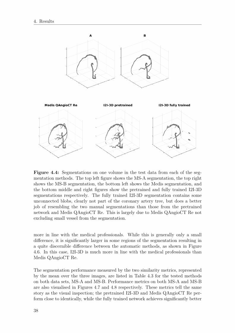
4. Results
Figure 4.4: Segmentations on one volume in the test data from each of the seg-mentation methods. The top left figure shows the MS-A segmentation, the top rightshows the MS-B segmentation, the bottom left shows the Medis segmentation, andthe bottom middle and right figures show the pretrained and fully trained I2I-3Dsegmentations respectively. The fully trained I2I-3D segmentation contains someunconnected blobs, clearly not part of the coronary artery tree, but does a betterjob of resembling the two manual segmentations than those from the pretrainednetwork and Medis QAngioCT Re. This is largely due to Medis QAngioCT Re notexcluding small vessel from the segmentation.
more in line with the medical professionals. While this is generally only a smalldifference, it is significantly larger in some regions of the segmentation resulting ina quite discernible difference between the automatic methods, as shown in Figure4.6. In this case, I2I-3D is much more in line with the medical professionals thanMedis QAngioCT Re.
The segmentation performance measured by the two similarity metrics, representedby the mean over the three images, are listed in Table 4.3 for the tested methodson both data sets, MS-A and MS-B. Performance metrics on both MS-A and MS-Bare also visualised in Figures 4.7 and 4.8 respectively. These metrics tell the samestory as the visual inspection; the pretrained I2I-3D and Medis QAngioCT Re per-form close to identically, while the fully trained network achieves significantly better
38

4. Results
Figure 4.5: Image highlighting segmentation border placement for segmentationsfrom professional A (top left), professional B (top right), Medis QAngioCT Re(bottom left), and the fully trained I2I-3D (bottom right). Area marked in redrepresents the segmentation.
similarity metrics. Over the three test images, the two professionals (i.e. the in-terobserver variability) achieve the highest similarity in both similarity measures.The fully trained I2I-3D network shows better performance and less variation thanMedis QAngioCT Re on both MS-A and MS-B.
Table 4.3: Similarity metrics measuring segmentation performance. A high DIas well as a low mHD are desired. The I2I-3D network can not compete with theinterobserver agreement, but outperforms the non-deep learning based automaticsoftware in similarity to both medical professionals.
Segmentation MS-A MS-Bmethod DI mHD DI mHD
Professional A - - 0.89 2.18Professional B 0.89 2.18 - -I2I-3D fully trained 0.73 3.51 0.74 3.47I2I-3D pretrained 0.57 4.63 0.58 4.57Medis QAngioCT Re 0.58 4.69 0.60 4.64
In addition to the fully trained I2I-3D, two networks trained solely on segmentationsfrom one of the professionals were also implemented, i.e. only having trained on MS-
39

4. Results
Figure 4.6: Image highlighting segmentation border placement for segmentationsfrom professional A (top left), professional B (top right), Medis QAngioCT Re(bottom left), and the fully trained I2I-3D (bottom right). Area marked in redrepresents the segmentation.
A and MS-B respectively. However, neither of these produced results on par withthe fully trained I2I-3D, and they are thus left out of the comparison.
40

4. Results
0.3
0.4
0.5
0.6
0.7
0.8
0.9
1
DI
(higher = better)
Professional B
I2I-3D fully trained
I2I-3D pretrained
Medis QAngioCT Re
0
1
2
3
4
5
6
7
8
9
10
mHD
(lower = better)
Professional B
I2I-3D fully trained
I2I-3D pretrained
Medis QAngioCT Re
Performance on
data set MS-A
Figure 4.7: Performance of segmentation methods on the three images in data setMS-A. Professional B shows both the best performance and the least variation in DI.In mHD, B has the best performance, but I2I-3D shows the least variation. Whileprofessional B achieves the best results, the fully trained I2I-3D does outperformMedis QAngioCT Re, whereas the pretrained I2I-3D is close to Medis QAngioCTRe’s performance.
0.3
0.4
0.5
0.6
0.7
0.8
0.9
1
DI
(higher = better)
Professional A
I2I-3D fully trained
I2I-3D pretrained
Medis QAngioCT Re
0
1
2
3
4
5
6
7
8
9
10
mHD
(lower = better)
Professional A
I2I-3D fully trained
I2I-3D pretrained
Medis QAngioCT Re
Performance on
data set MS-B
Figure 4.8: Performance of segmentation methods on the three images in dataset MS-B. Once again, the professional shows the best segmentation performance,followed by the I2I-3D network. The fully trained network shows better performanceand less variation than the Medis QAngioCT Re software. The pretrained I2I-3D isclose to Medis QAngioCT Re in performance.
41

4. Results
42

5Discussion
5.1 Analysis of methodThis study investigated the coronary artery segmentation performance of a version ofthe I2I-3D network implemented in PyTorch. By building the network from scratchin PyTorch rather than using the Caffe implementation provided by Merkow et al.,a significant amount of time was consumed by implementing and testing the net-work. Had a different methodology been chosen, for example starting from the Caffeimplementation, this project could most likely have reached further in the investi-gation of the network’s potential. There could also have been time to investigateimprovements to the architecture of the network. That said, there is also value inproviding an implementation of the network in another framework1, expanding itsavailability for further research. With the network showing promising performance,that value should not be neglected.
A limiting factor of this project is the relatively small data sets. With a test set ofonly three images in the main data set, one could certainly question the weight ofthe results. A clear indication that the data sets were too small was shown in Tables4.1 and 4.2, where the performance was better on the AS and MS validation setsthan on the respective training sets. Since the network has trained on the trainingset but never seen the validation images, one expects the performance to be higheron the training set than on the validation set. That fact that it is not may be anindication that some hard to learn features in the training sets were not representedin the validation sets. To do the evaluation thoroughly would thus require a largerdata set. With the SCAPIS study progressing, that will become a reality in time.Working with medical data, as that provided by SCAPIS, requires that ethical con-cerns are taken into consideration. It should not be possible to connect any datasample to an individual taking part in the study. As such, the data used in thisproject was stripped of identification tags in information headers.
Another data set that could have been used as either another pretraining data set oranother evaluation set is from the Rotterdam Coronary Artery Algorithm EvaluationFramework which provides data to compare methods for coronary artery segmenta-tion and stenoses detection [23]. Using this data would have been the next step inthe investigation into I2I-3D’s potential, given more time. With facts in hand, thatwould have been a better use of time than that spent trying to implement mixed
1Available at https://github.com/frefdrk/i2i3d-pytorch
43

5. Discussion
precision learning.
Why attempts to implement mixed precision were unsuccessful is not known. Asthe network was not able to learn with mixed precision, there might have been aproblem of vanishing gradients, i.e. gradients being too small to affect parametersin the update. One parameter in mixed precision learning, the loss scaling factor,should be tuned to combat this problem and that might not have been done correctly.
5.2 Analysis of resultsWith the I2I-3D network architecture having performed well on vessel wall bound-ary detection in prior research, it is expected that it is also able to learn to segmentfull vessel structures. However, with relatively low filter sizes of only 4, 8, 16 and 32layers in the four respective filter blocks it is surprisingly effective at the task, ableto outperform a commercial automatic software in similarity metrics measured tomanual segmentations. On one hand, this is showing impressive performance. Onthe other hand, when analysing the segmentations in Figure 4.4 by eye one can seethat Medis QAngioCT Re is better at keeping vessel structures intact, and its mainfault is including the small, clinically irrelevant vessels of a diameter below 2 mm.The fully trained network, having learnt to not include these, has the upper hand inthat regard. Even with the impressive numbers in Table 4.3, one should not be toohasty in celebrating the performance of the network when compared to QAngioCTRe. The similarity metrics do not tell the complete story.
A more fair comparison of how the two automatic methods compare in full coro-nary artery vessel segmentation is shown in Figure 4.3. Clearly, the network canproduce segmentations similar to Medis QAngioCT Re, but that was not the goalof this study. This study aims to reach beyond the Medis QAngioCT Re’s seg-mentations and produce segmentations as close to the manual ones as possible.The network suceeds in that aspect. During the training on the manual segmenta-tions, the network learns to disregard the small vessels that Medis QAngioCT Reincludes, although not perfectly, which improves the similarity indices to manualsegmentations quite drastically. The network also learns to place the segmentationborder more in line with the manual segmentations than Medis QAngioCT Re, asshown in Figures 4.5 and 4.6. These are both improvements that could set aparta deep learning approach from regular automatic approaches. However, it seemsthat what the network learns when training on the manual data unfortunately alsoresults in there being broken vessels, as can be seen in the left most vessel in Figure4.4. There are ways to combat this issue. Using more manually segmented train-ing data could be a first step, for example. Post-processing on the probabilisticnetwork output could also be applied. As an example, applying Frangi filteringtechniques to detect vessel-like structures in the probabilistic output might producemore sophisticated segmentations than simply thresholding at 0.5. Other alterna-tives for post-processing include using connected component analysis to distinguishlarge connected components (vessels) from small connected components (non-vessel
44

5. Discussion
blobs), using conditional random field modeling to produce segmentations from lo-cal information in the probabilistic output rather than thresholding every voxel ata fix threshold, and to simply exclude any structures smaller than 2 mm in diameter.
Nevertheless, using a state-of-the-art network architecture, designed for use on med-ical images and for vessel (wall) segmentation in the form of I2I-3D, gives promisingresults. While not quite keeping up with medical professional segmentations, thesimilarity measures favour the deep learning approach over commercial segmentationsoftware. A deep learning method for coronary artery segmentation, as suggestedin this thesis, definitely seems viable.
In addition to this, it is important to remember that these results were achievedusing a rather limited data set. With 77 automatic coronary artery segmentationsin pretraining and 25 manually corrected segmentations for the main training, theseresults show great potential in regards to what could be possible to achieve with alarger data set. That said, any results obtained with such a small evaluation set,three images in this case, should be taken with a grain of salt as pointed out previ-ously. Nevertheless, the strong ability of the U-shaped, interconnected fully convolu-tional network with integration of deep supervision, but otherwise quite bare-bonedstructure, to segment these tiny structures in the evaluation data from limited andhighly unbalanced data sets should be encouraging for future work.
None of the data used to train the network is published online. It was generouslymade available from the SCAPIS project for this specific study, meaning that testingthe repeatability of the results achieved in the thesis is limited to those connectedto the SCAPIS project.
Finally, a point regarding the proposed method for coronary artery segmentationin this thesis should be made clear; the proposed deep learning tool aims to assistmedical professionals in their work rather than to replace them altogether. Thesegmentation results and, in continuation, any diagnoses based on them should beinspected by a professional.
5.3 Subjectivity in manual segmentationsThe similarity metrics between the medical professionals segmentations verify thesubjectivity in the process of producing manual segmentations mentioned in Sec-tion 3.1.4. With a Dice index of 0.89 and a modified Hausdorff distance of 2.18 inthe test data set, it is clear that they differ, although not to a huge degree. Thequestion of how a neural network handles such subjectivity in the training data isinteresting. Looking at Figure 4.4, the network looks to be more similar to the seg-mentation from professional B than that from professional A in the presented case,which the similarity metrics agree with. Whether the subjectivity in the data is aproblem or not is difficult to answer. Since medical professionals don’t completelyagree on what the ground truth is in terms of segmentations, the most one can hopeof from the network is that it produces segmentations that are more similar to the
45

5. Discussion
group of medical professionals than any one professional from that group. With theprofessionals each having their own subjective ideal segmentation, the network willnever be able to agree completely with all of them. This needs to be understood byanyone wanting to use a deep learning tool in this fashion. Alternatively, one couldconstruct a separate network for each individual. The subjectivity would still bepresent, but there would only be the subjectivity of one individual to learn. Thiswas attempted in this project, but did not result in segmentations on par with thenetwork trained on both MS-A and MS-B on either of the MS-A or MS-B test datasets. Either way, if the tool is to be used to produce an automatic segmentation tothen manually correct, having the tool produce some sort of average segmentationin relation to a large group of medical professionals seems like the way to go froman engineer’s point of view.
5.4 Future workWith the SCAPIS study advancing, more and more segmentation data will be pro-duced. This could certainly benefit deep learning algorithms which are so deeplydependent on training data. With a starting point in the proposed I2I-3D network,there are also additions and changes to be investigated. A successful implementa-tion of mixed precision training would allow for a deeper network which potentiallycould improve the network performance. The architecture does not include eitherbatch normalisation layers or drop-out layers, as Merkow et al. did not include thesein their original architecture, both of which have shown to have a positive impacton learning [44] [6]. Modified versions of the ReLU activation function, such as theLeaky ReLU which has a non-zero response for negative inputs, have also shownimprovements compared to regular ReLU in CNN applications [45].
These points, together with hyperparameter optimisation and post-processing pos-sibilities previously mentioned clearly show that there is still a lot of potential toinvestigate. With deep learning based segmentation of coronary arteries being thefirst step in the development of a larger tool, this should be done thoroughly.
Building on this deep learning approach to construct a deep learning based tool ableto detect stenosis and vascular plaque is a vision of the Computer Vision and MedicalImage Analysis group at the Department of Electrical Engineering at ChalmersUniversity of Technology. Using the proposed I2I-3D structure can be encouragedbased on the results of this thesis.
46

6Conclusion
In a large-scale study such as SCAPIS, it is important that the automatic segmenta-tion tools used are able to produce high-quality segmentations in order to minimisethe need for laborious and time consuming manual correction. The field of au-tomated image analysis has been moving away from traditional image processingtechniques in favour of deep learning for some time now. In the case of image seg-mentation, fully convolutional networks are leading the way, with U-Net inspirednetworks such as I2I-3D being front runners in medical applications.
The main research question of this thesis is whether or not a deep learning methodfor coronary artery segmentation in CTA images is viable. To answer that ques-tion, a version of the state-of-the-art deep convolutional neural network architecturenamed I2I-3D was applied to data from the SCAPIS study. The network was imple-mented in the PyTorch deep learning framework, with pretraining on three separatedata sets. To investigate the viability, the network segmentations were comparedto both commercial segmentation software and manual segmentations performed bytwo medical professionals. The comparison was made by establishing how similar thedifferent methods were to each of the manual segmentations through two separatesimilarity metrics. One metric, Dice index, measures the segmentation overlap, i.e.counts correctly and incorrectly classified voxels and gives a single value correspond-ing to the performance. The other metric, modified Hausdorff distance, determineshow close in space two segmentations are, i.e. determining similarity in overall shape.
What can be concluded from the results is:1. The I2I-3D network is able to learn well from the limited data set but can not
perform on par with manual segmentations.2. The I2I-3D network beats the commercial software Medis QAngioCT Re in
both similarity measures on both evaluation data sets. Manual inspection ofthe segmentation shows that the network loses some important structures ofthe coronary tree, making it harder to determine a clear winner between thetwo. The largest source of dissimilarity between the manual segmentation andMedis QAngioCT Re segmentations is that the latter includes small vesselstructures, while the former does not. I2I-3D does however perform better insegmentation border placement than Medis QAngioCT Re.
3. The results are promising for future development, as there are clear additionsand changes to investigate for potential improvements, such as batch normal-isation layers, drop-out layers and post-processing of the probabilistic outputfrom the network.
47

6. Conclusion
The main research question of this thesis was: Is deep learning viable for coronaryartery segmentation? With the network outperforming the commercial software inboth similarity metrics, the viability has been demonstrated. However, a visual in-spection of the segmentations show that there is still room for improvement. Withmore data and implementation of the proposed additions possibly improving theperformance further, the future for a deep learning based coronary artery segmen-tation tool looks bright.
48

Bibliography
[1] Geneva: World Health Organization. World health statistics 2017: Monitoringhealth for the SDGs, sustainable development goals. 2017.
[2] G. Bergström et al. The Swedish Cardiopulmonary Bioimage Study: Objectivesand Design. Journal of internal medicine, 278(6):645–659, 2015.
[3] A. Broersen et al. FrenchCoast: Fast, robust extraction for the nice challenge oncoronary artery segmentation of the tree. In Proceedings of MICCAI Workshop”3D Cardiovascular Imaging: a MICCAI segmentation Challenge, 2012.
[4] P. Fischer O. Ronneberger and T. Brox. U-Net: Convolutional Networks forBiomedical Image Segmentation. CoRR, abs/1505.04597, 2015.
[5] J. Merkow et al. Dense volume-to-volume vascular boundary detection. CoRR,abs/1605.08401, 2016.
[6] Y. Bengio Y. LeCun and G. Hinton. Deep learning. Nature, 521(7553):436,2015.
[7] David E Rumelhart, Geoffrey E Hinton, and Ronald J Williams. Learningrepresentations by back-propagating errors. Nature, 323(6088):533, 1986.
[8] N. Srivastava et al. Dropout: A simple way to prevent neural networks fromoverfitting. The Journal of Machine Learning Research, 15(1):1929–1958, 2014.
[9] A. Krogh and J. A. Hertz. A simple weight decay can improve generalization.In Advances in neural information processing systems, pages 950–957, 1992.
[10] D. P. Kingma and J. Ba. Adam: A method for stochastic optimization. arXivpreprint arXiv:1412.6980, 2014.
[11] C. Lee. Deeply-supervised nets. In Artificial Intelligence and Statistics, pages562–570, 2015.
[12] S. J. Pan and Q. Yang. A survey on transfer learning. IEEE Transactions onknowledge and data engineering, 22(10):1345–1359, 2010.
[13] K. Fukushima and S. Miyake. Neocognitron: A self-organizing neural networkmodel for a mechanism of visual pattern recognition. In Competition and co-operation in neural nets, pages 267–285. Springer, 1982.
[14] S. Ji et al. 3D convolutional neural networks for human action recognition.
49

Bibliography
IEEE Transactions on Pattern Analysis and Machine Intelligence, 35(1):221–231, Jan 2013.
[15] O. Russakovsky et al. ImageNet Large Scale Visual Recognition Challenge.International Journal of Computer Vision (IJCV), 115(3):211–252, 2015.
[16] UNC Vision Lab ImageNet. Large scale visual recognition challenge 2017(ilsvrc2017), 2017. URL http://image-net.org/challenges/LSVRC/2017/results. [Online; accessed 3 May 2018].
[17] S. Beucher et al. The watershed transformation applied to image segmentation.Scanning Microscopy-Supplement, pages 299–299, 1992.
[18] Y. Huang and D. Chen. Watershed segmentation for breast tumor in 2-Dsonography. Ultrasound in Medicine and Biology, 30(5):625–632, 2004.
[19] A. Frangi et al. Multiscale vessel enhancement filtering. In William M.Wells, Alan Colchester, and Scott Delp, editors, Medical Image Computing andComputer-Assisted Intervention — MICCAI’98, pages 130–137, Berlin, Heidel-berg, 1998. Springer Berlin Heidelberg.
[20] M. E. Martinez-Perez et al. Segmentation of blood vessels from red-free andfluorescein retinal images. Medical image analysis, 11(1):47–61, 2007.
[21] H. K. Yuen et al. Comparative study of hough transform methods for circlefinding. Image and vision computing, 8(1):71–77, 1990.
[22] M Schaap et al. Standardized evaluation methodology and reference databasefor evaluating coronary artery centerline extraction algorithms. Medical ImageAnalysis, 13(5):701 – 714, 2009. Includes Special Section on the 12th Interna-tional Conference on Medical Imaging and Computer Assisted Intervention.
[23] Consortium for Open Medical Image Computing. Rotterdam coro-nary artery algorithm evaluation framework, 2018. URL http://coronary.bigr.nl/stenoses/results/results.php?type=testing&subs=public&sinfo=no&vendor=all. [Online; accessed 23 May 2018].
[24] D. Ciresan et al. Deep neural networks segment neuronal membranes in electronmicroscopy images. In F. Pereira, C. J. C. Burges, L. Bottou, and K. Q.Weinberger, editors, Advances in Neural Information Processing Systems 25,pages 2843–2851. Curran Associates, Inc., 2012.
[25] N Feng et al. Toward automatic phenotyping of developing embryos from videos.IEEE Transactions on Image Processing, 14(9):1360–1371, 2005.
[26] E. Shelhamer J. Long and T. Darrell. Fully convolutional networks for semanticsegmentation. In Proceedings of the IEEE conference on computer vision andpattern recognition, pages 3431–3440, 2015.
[27] Ö. Çiçek et al. 3D u-net: learning dense volumetric segmentation from sparseannotation. In International Conference on Medical Image Computing andComputer-Assisted Intervention, pages 424–432. Springer, 2016.
50

Bibliography
[28] O. Jimenez del Toro et al. Cloud-based evaluation of anatomical structure seg-mentation and landmark detection algorithms: Visceral anatomy benchmarks.35(11):2459–2475, 2016.
[29] A. Norlén et al. Automatic pericardium segmentation and quantification ofepicardial fat from computed tomography angiography. Journal of MedicalImaging, 3(3):034003, 2016.
[30] Y. LeCun et al. Efficient backprop. In Neural networks: Tricks of the trade,pages 9–50. Springer, 1998.
[31] M. Eichelberg P. Mildenberger and E. Martin. Introduction to the dicom stan-dard. European Radiology, 12(4):920–927, Apr 2002.
[32] E. Jones et al. SciPy: Open source scientific tools for Python, 2001–. URLhttp://www.scipy.org/. [Online; accessed 30 Apr 2018].
[33] The PyTorch Team. Pytorch, a year in..., 2018. URL http://pytorch.org/2018/01/19/a-year-in.html. [Online; accessed 30 Apr 2018].
[34] A Paszke. Automatic differentiation in pytorch. 2017.
[35] N. Ketkar. Introduction to PyTorch, pages 195–208. Apress, Berkeley, CA,2017.
[36] jmerkow. Github user page, 2016. URL https://github.com/jmerkow/I2I/.[Online; accessed 30 Apr 2018].
[37] NVIDIA. Training with mixed precision :: Deep learning sdk documen-tation, 2018. URL https://docs.nvidia.com/deeplearning/sdk/mixed-precision-training/index.html. [Online; accessed 13 May 2018].
[38] X. Glorot and Y. Bengio. Understanding the difficulty of training deep feedfor-ward neural networks. In Proceedings of the thirteenth international conferenceon artificial intelligence and statistics, pages 249–256, 2010.
[39] A. A. Taha and A. Hanbury. Metrics for evaluating 3D medical image segmen-tation: Analysis, selection, and tool. BMC medical imaging, 15(1):29, 2015.
[40] K. Zou et al. Statistical validation of image segmentation quality based on aspatial overlap index1. Academic Radiology, 2(11):178–189, 2004.
[41] K. Zou et al. Three validation metrics for automated probabilistic image seg-mentation of brain tumours. Statistics in medicine, 23(8):1259–1282, 2004.
[42] R. de Luis-García R. Cárdenes and M. Bach-Cuadra. A multidimensional seg-mentation evaluation for medical image data. Computer methods and programsin biomedicine, 96(2):108–124, 2009.
[43] M. Dubuisson and A. K. Jain. A modified hausdorff distance for object match-ing. In Pattern Recognition, 1994. Vol. 1-Conference A: Computer Vision &Image Processing., Proceedings of the 12th IAPR International Conference on,volume 1, pages 566–568. IEEE, 1994.
51

Bibliography
[44] S. Ioffe and C. Szegedy. Batch normalization: Accelerating deep network train-ing by reducing internal covariate shift. arXiv preprint arXiv:1502.03167, 2015.
[45] B. Xu et al. Empirical evaluation of rectified activations in convolutional net-work. arXiv preprint arXiv:1505.00853, 2015.
52

ASegmentations for the three test
volumes in the MS dataset
I

A. Segmentations for the three test volumes in the MS dataset
Figure A.1: Volume #1 in test set of the MS dataset.
II

A. Segmentations for the three test volumes in the MS dataset
Figure A.2: Volume #2 in test set of the MS dataset.
III

A. Segmentations for the three test volumes in the MS dataset
Figure A.3: Volume #3 in test set of the MS dataset.
IV