1

DEEP LEARNING FOR EXOTIC OPTION VALUATION*

Jay Cao, Jacky Chen, John Hull, Zissis Poulos

Abstract

A common approach to valuing exotic options involves choosing a model and then determining its

parameters to fit the volatility surface as closely as possible. We refer to this as the model

calibration approach (MCA). A disadvantage of MCA is that some information in the volatility

surface is lost during the calibration process and the prices of exotic options will not in general be

consistent with those of plain vanilla options. We consider an alternative approach where the

structure of the user’s preferred model is preserved but points on the volatility are features input to

a neural network. We refer to this as the volatility feature approach (VFA) model. We conduct

experiments showing that VFA can be expected to outperform MCA for the volatility surfaces

encountered in practice. Once the upfront computational time has been invested in developing the

neural network, the valuation of exotic options using VFA is very fast.

*An earlier version of this paper was titled “Valuing exotic options and estimating model risk”

2

DEEP LEARNING FOR EXOTIC OPTION VALUATION

For many underlying assets, there is little uncertainty about the pricing of plain vanilla

European and American options. Quotes and trades by market participants provide points on the

volatility surface. Interpolating between these points as necessary, a trader can derive a reasonable

estimate of the implied volatility appropriate for any new plain vanilla European or American

option that is of interest. Plain vanilla options are therefore not priced using a model. They are

simply priced to be consistent with the market. The volatility surface derived from the Black–

Scholes–Merton model is a convenient interpolation tool for doing this.

Exotic options are generally not as actively traded as plain vanilla options and, as a result, a

model is required for pricing. A variety of different models are used in practice. Two conditions

that traders would like the model to satisfy are:

A. The stochastic behavior assumed for the underlying asset price should correspond

reasonably well to its observed behavior, and

B. The volatility surface derived from the model should be reasonably consistent with the

volatility surface used to price plain vanilla options.

Two categories of models that are used in practice can be distinguished. The models in the first

category focus on condition A by assuming a process for the asset price that is roughly consistent

with its observed behavior. The models have parameters that can be chosen to provide an

approximate fit to the current volatility surface. Models in the second category focus on condition B

and are designed to be exactly consistent with the current volatility surface.

Many different models in the first category involving stochastic volatility and jumps have been

proposed. Examples of stochastic volatility models are Hull and White (1987) and Heston (1993).

Merton (1976) proposed a model that overlays Black-Scholes-Merton model with jumps. Bates

(1996) adds jumps to Heston (1993). Madan et al (1998) propose a variance–gamma model where

there are only jumps. More recently, rough volatility models where the process for volatility is

non-Markov have been suggested by authors such as Gatheral et al (2018).

The second category of models are referred to as local volatility models. The original one-

factor local volatility model was suggested by Dupire (1994) and Derman and Kani (1994). It has

3

been extended by authors such as Ren et al (2007) and Saporito et al (2019). Local volatility

models by design satisfy condition B. However, they are liable to perform less well than models in

the first category as far as condition A is concerned.

This paper is concerned with ways in which machine learning can be used to bridge the gap

between the two categories of models. It provides a way in which models in the first category can

be made more consistent with the volatility surface, and therefore with the pricing of plain vanilla

options.

The usual approach to implementing models in the first category is to choose model

parameters to fit the volatility surface as closely as possible. This approach, which we refer to as

the “model calibration approach” or MCA has been used by researchers such as Horvath et al

(2021) and Liu et al (2019). A drawback of the approach is that some of the points on the volatility

surface are likely to be more important than others for any particular exotic option that is

considered. It is of course possible to vary the weights assigned to different points on the volatility

surface according to the instrument being valued. However, it is difficult to determine in advance

what these weights should be. As a result, the points are usually given equal weight when model

parameters are determined.

Authors such as Ferguson and Green (2018) show how neural networks can be used in

conjunction with MCA to provide fast pricing once model parameters have been determined.

Consider an exotic option that is valued using Monte Carlo simulation. As a first step, it is necessary

to devote computational resources to creating a data set relating model parameters and exotic

option parameters to the price. The pricing model can then be replicated with a neural network.

Once this has been done, valuation is several orders of magnitude faster than Monte Carlo

simulation because it involves nothing more than a forward pass through the neural network.

We suggest an approach, which we refer to as the “volatility feature approach” or VFA. This can

be regarded as an extension of the Ferguson and Green (2018) methodology. We create a neural

network where the inputs are the volatility surface points and the exotic option parameters and the

target is the price. We randomly generate many sets of parameters for (a) the model under

consideration and (b) the exotic option under consideration. For each set of parameters, a volatility

surface and a price for the exotic option are calculated. The neural network is then constructed.

The model parameters are used to create the training set, but they are not inputs to the neural

network.

4

The VFA approach is a compromise between models that satisfy condition A and those that

satisfy condition B. It retains some of the structure of an analyst’s preferred model while learning

which points on the volatility surface are most important for the exotic option being valued. It

produces prices for exotic options that are more consistent with the prices of vanilla options than

MCA.1

We first carry out an experiment to compare the performance of MCA and VFA. We assume that

the world is governed by a particular model A, and that the model used for pricing a particular type

of exotic option is an alternative simpler model B. The ‘true’ prices of a panel of exotic options are

determined using model A. The average pricing errors of VFA and MCA are about the same in the

experiment. However, a key result is that the performance of VFA relative to MCA increases

significantly as the MCA calibration error increases. For the volatility surfaces encountered in

practice, the calibration error is on average much greater than in our idealized experiment. This

provides evidence suggesting that VFA is a better tool than MCA.

As a second test, we compare the pricing of knock-in and knock-out options with vanilla

options. A portfolio consisting of a knock-in and a knock-out option with the same barrier level,

strike price and maturity should, in the absence of arbitrage, have the same value as a vanilla

European option with that strike price and maturity. Using S&P 500 data, we show that this is much

closer to being true for VFA than MCA.

Model risk has assumed increasing importance for both dealers and their regulators in recent

years. SR 11-7, which was published by the U.S. Board of Governors of the Federal Reserve System

in 2011, and is used by other regulators throughout the world, requires banks to identify sources of

model risk and carry out frequent model validation exercises.2 We illustrate how model risk can be

assessed using VFA for options on the S&P 500 by comparing Bates (1996) and a version of the

rough volatility model.

1 Unlike MCA, VFA model is not necessarily an arbitrage-free model. This means that there may be theoretical arbitrage opportunities between the pricing of different exotic options. However, this disadvantage is outweighed by the fact that VFA creates less arbitrage opportunities between exotic and vanilla options than MCA. 2 See Federal Reserve System (2011)

5

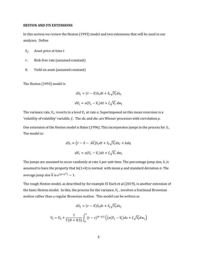
HESTON AND ITS EXTENSIONS

In this section we review the Heston (1993) model and two extensions that will be used in our

analyses. Define

𝑆𝑡: Asset price at time t

r: Risk-free rate (assumed constant)

δ: Yield on asset (assumed constant)

The Heston (1993) model is

𝑑𝑆𝑡 = (𝑟 − 𝛿)𝑆𝑡𝑑𝑡 + 𝑆𝑡√𝑉𝑡𝑑𝑧𝑡

𝑑𝑉𝑡 = 𝑎(𝑉𝐿 − 𝑉𝑡)𝑑𝑡 + 𝜉√𝑉𝑡 𝑑𝑤𝑡

The variance rate, 𝑉𝑡 , reverts to a level 𝑉𝐿 at rate a. Superimposed on this mean reversion is a

‘volatility of volatility’ variable, 𝜉. The dzt and dwt are Wiener processes with correlation ρ.

One extension of the Heston model is Bates (1996). This incorporates jumps in the process for St.

The model is:

𝑑𝑆𝑡 = (𝑟 − 𝛿 − 𝜆�̅�)𝑆𝑡𝑑𝑡 + 𝑆𝑡√𝑉𝑡𝑑𝑧𝑡 + 𝑘𝑑𝑞

𝑑𝑉𝑡 = 𝑎(𝑉𝐿 − 𝑉𝑡)𝑑𝑡 + 𝜉√𝑉𝑡 𝑑𝑤𝑡

The jumps are assumed to occur randomly at rate λ per unit time. The percentage jump size, k, is

assumed to have the property that ln(1+k) is normal with mean μ and standard deviation σ. The

average jump size �̅� is 𝑒(𝜇+𝜎2) − 1.

The rough Heston model, as described by for example El Euch et al (2019), is another extension of

the basic Heston model. In this, the process for the variance, 𝑉𝑡 , involves a fractional Brownian

motion rather than a regular Brownian motion. This model can be written as

𝑑𝑆𝑡 = (𝑟 − 𝛿)𝑆𝑡𝑑𝑡 + 𝑆𝑡√𝑉𝑡𝑑𝑧𝑡

𝑉𝑡 = 𝑉0 +1

Γ(𝐻 + 0.5)∫ (𝑡 − 𝑠)𝐻−0.5 ((𝑎(𝑉𝐿 − 𝑉𝑠)𝑑𝑠 + 𝜉√𝑉𝑠𝑑𝑤𝑠)

𝑡

0

6

where the correlation between dzt and dwt is ρ, H is the Hurst exponent, and Γ is the gamma

function. When H = 0.5 the model reduces to Heston (1993). When H < 0.5, the correlation between

volatility movements in successive periods of time is negative while, when H > 0.5, this correlation

is positive. Gatheral et al (2018) produce results for indices showing that the model reflects market

data well when H is between 0.06 and 0.20.

A close approximation to the rough Heston model is the lifted Heston model proposed by Jaber

(2019). This has the advantage that it involves only regular Brownian motions and, as a result, is

much faster for the computation of exotic option prices. We will use the following version of Jaber

(2019)

𝑑𝑆𝑡 = (𝑟 − 𝛿)𝑆𝑡𝑑𝑡 + 𝑆𝑡√𝑉𝑡𝑑𝑧𝑡

𝑉𝑡 = 𝑉0 + 𝑎𝑉𝐿 ∑𝑐𝑖

𝑥𝑖

(1 − 𝑒−𝑥𝑖𝑡)

𝑛

𝑖=1

+ ∑ 𝑐𝑖𝑈𝑖,𝑡

𝑛

𝑖=1

𝑑𝑈𝑖,𝑡 = −𝑥𝑖𝑈𝑖,𝑡𝑑𝑡 + 𝜉√𝑉𝑡𝑑𝑤𝑡

where the correlation between the Wiener processes, dzt and dwt , is ρ. The Ui,t are initially zero and

revert to zero at different speeds 𝑥𝑖 .

As recommended by Jaber, we set n = 20 and

𝑐𝑖 =(𝛽1−𝛼 − 1)𝛽(𝛼−1)(1+

𝑛2

)

𝛤(𝛼)𝛤(2 − 𝛼)𝛽(1−𝛼)𝑖

𝑥𝑖 = (1 − 𝛼

2 − 𝛼) (

𝛽2−𝛼 − 1

𝛽1−𝛼 − 1)𝛽𝑖−1−

𝑛2

with α = H + 0.5 and 𝛽 = 2.5.

A CONTROLLED EXPERIMENT

In this section, we describe a controlled experiment to compare the results from MCA and VFA.

We assume that an asset price evolves according to a particular model A and that a simpler model B

is used for pricing a particular type of exotic option dependent on the asset price. The ‘true’ prices

of a panel of exotic options are determined using model A. The prices using both MCA and VFA in

conjunction with model B are then computed and the accuracies of the models compared.

7

We define the volatility surface by considering five different times to maturity (one month,

three months, six months, one year, and two years) and five different strike prices (0.7S, 0.85S, S,

1.15S and 1.3S, where S is the asset price). When combined, these maturity/moneyness

combinations give 25 ‘standard’ points on the volatility surface. The MCA calibration error is

calculated as the minimum value of

𝑋 =1

25∑ |𝜎𝑗 − 𝜎𝑗

∗| 25

𝑗=1(1)

where 𝜎𝑗∗ is the ‘true’ implied volatility calculated from model A and 𝜎𝑗 is implied volatility at the jth

point on the volatility surface given by a set of model B parameters.

The steps in carrying out the controlled experiment are as follows:

(a) Sample n sets of parameters for model A and the exotic option under consideration.

(b) For each of the n scenarios in (a), calculate the 25 implied volatilities that define the ‘true’

volatility surface.

(c) For each of the n scenarios, calculate the parameters of model B that fit the 25 volatilities

calculated in (b) as closely as possible by using an iterative procedure that minimizes the

calibration error in equation (1).

(d) Calculate prices for the n exotic options in (a) using both model A and the calibrated model B in

(c).

(e) For each of the n scenarios, calculate the MCA error as the absolute value of the difference

between the two model prices.

(f) Sample N sets of parameters for model B and the exotic option under consideration. For each,

calculate the value of the exotic option and the 25 standard points on the volatility surface.

(g) Use the data from step (f) to construct a neural network where the features are the volatility

surface points and the exotic option parameters and the target is the model B exotic option

price.

(h) Use the neural network in (g) to calculate the prices of the n exotic options in (a) using the ‘true’

volatility surface in (b).

(i) For each of the n options in (a), calculate the VFA error as the absolute value of the difference

between the price in (h) and the model A price.

8

The neural networks we used in the experiment consisted of three hidden layers with 30

neurons per layer, and used the sigmoid activation function. We used Adam as the optimizer and

mean absolute error to measure training loss. In the training process, we saved the weights of the

neural network every time when the validation loss reached a new low. We stopped the training

when there was no improvement in the validation loss for 50 epochs and used the last saved set of

weights as the final weights of the model.

We assumed that model B (the valuation model) is Heston (1993) and model A (the ‘true

model’) is Bates (1996). We considered three different types of exotic options. The first is a knock-

out barrier call option where the barrier level is greater than either the initial asset price or the

strike price. The second is an Asian option where the payoff is the excess of the average asset price

during the life of the option over the strike price if this is positive and zero otherwise. The third is a

lookback option where the payoff is the excess of the highest price during the life of the option over

the strike price if this is positive and zero otherwise.

We set n=1,000 and N= 20,000, and used Monte Carlo simulation with 50,000 paths to calculate the

prices of the exotic options in (d) and (f).

We assumed an initial asset price, 𝑆0, of 100, a yield on the asset, δ, of zero, and sampled other

parameters from uniform distributions. We will denote the ranges considered by parentheses. For

example, [1, 2] indicates a uniform distribution between 1 and 2.

The model B (Heston) parameters in (f) were sampled as follows

Risk-free rate, r: [0.01, 0.05]

Initial variance, 𝑉0: [0.01, 0.25]

Mean reversion parameter, a: [0.1, 3]

Long-term variance, 𝑉𝐿: [0.01, 0.25]

Volatility of volatility, ξ: [0.1, 0.8]

Correlation, ρ: [–0.9, 0]

The model A (Bates) parameters in (a) were sampled similarly with the following additional

samples:

Jump intensity, λ: [1, 5]

Jump size parameter, 𝜇: [–0.05, 0.05]

Jump size parameter, σ: [0, 0.05]

9

The option parameters in (a) and (f) were sampled as follows:

Time to maturity (yrs): [0.05, 2]

Strike price: [80, 120]

For barrier options, the barrier level was set equal to C times the maximum of the asset price and

strike price with C sampled from [1.05, 1.30].

Define Y as the MCA minus the VFA error. We plotted Y against the calibration error, X, in equation

(1). The results are shown in Exhibit 1. Overall VFA performed only slightly better than MCA, but

the t-statistics indicate that as the calibration error increases the performance of VFA relative to

MCA improves significantly. This result is not too surprising. When the model provides a good fit to

the volatility surface MCA performs well. As the fit becomes worse, VFA starts to perform relatively

better because it retains all information about the volatility surface.

Exhibit 1: Results of regressing the MCA error minus the VFA error (Y) against the MCA calibration

error (X). t-statistics are in parentheses.

Exotic Option Relationship

Barrier 𝑌 = −0.10 + 16.35𝑋

(−8.30) (15.64)

Asian 𝑌 = −0.21 + 10.37𝑋

(−17.90) (9.96)

Lookback 𝑌 = −0.42 + 58.42𝑋

(−11.41) (18.04)

The results are encouraging. The Bates model is an extension of Heston and shares many of its

properties. The volatility surfaces encountered in practice can be expected to be ‘less well behaved’

than those derived from the Bates model. To investigate this, we fitted Heston to S&P 500 volatility

surfaces between 2001 and 2019. As will be described later, the volatility surface was defined

10

using 19 rather than 25 standard points and the points were determined from market data using a

bivariate linear interpolation.

We found the S&P 500 calibration errors to be over twice as high on average as the Bates

calibration errors. Given that the relative performance of VFA improves as the calibration error

increases, our results suggest that VFA is likely to be a better tool than MCA in practice.3 Once the

upfront computational time to create the neural network has been invested, VFA provides a fast

pricing tool.4

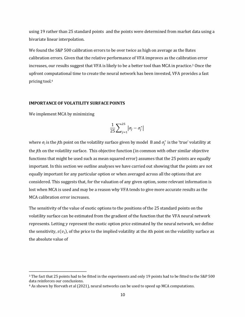
IMPORTANCE OF VOLATILITY SURFACE POINTS

We implement MCA by minimizing

1

25∑ |𝜎𝑗 − 𝜎𝑗

∗|25

𝑗=1

where σj is the jth point on the volatility surface given by model B and 𝜎𝑗∗ is the ‘true’ volatility at

the jth on the volatility surface. This objective function (in common with other similar objective

functions that might be used such as mean squared error) assumes that the 25 points are equally

important. In this section we outline analyses we have carried out showing that the points are not

equally important for any particular option or when averaged across all the options that are

considered. This suggests that, for the valuation of any given option, some relevant information is

lost when MCA is used and may be a reason why VFA tends to give more accurate results as the

MCA calibration error increases.

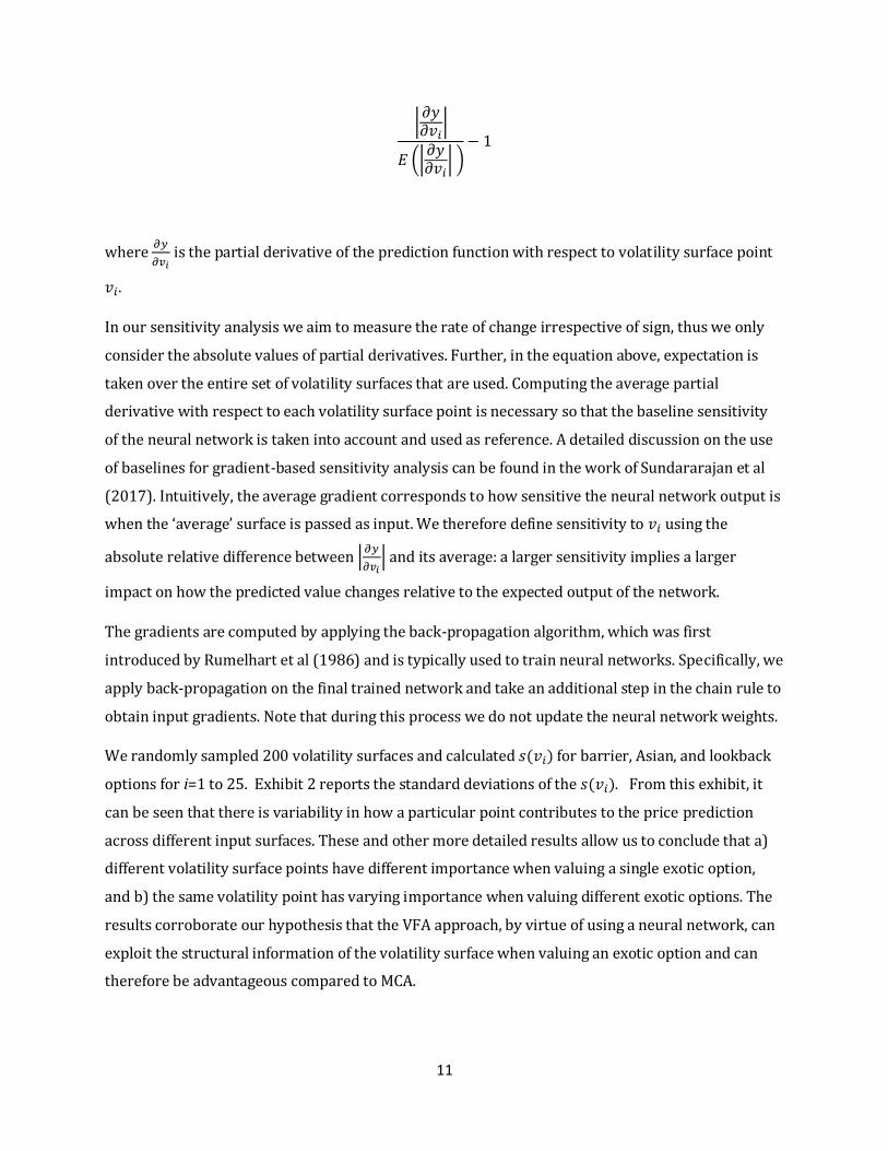
The sensitivity of the value of exotic options to the positions of the 25 standard points on the

volatility surface can be estimated from the gradient of the function that the VFA neural network

represents. Letting 𝑦 represent the exotic option price estimated by the neural network, we define

the sensitivity, 𝑠(𝑣𝑖), of the price to the implied volatility at the ith point on the volatility surface as

the absolute value of

3 The fact that 25 points had to be fitted in the experiments and only 19 points had to be fitted to the S&P 500 data reinforces our conclusions. 4 As shown by Horvath et al (2021), neural networks can be used to speed up MCA computations.

11

|𝜕𝑦𝜕𝑣𝑖

|

𝐸 (|𝜕𝑦𝜕𝑣𝑖

| )− 1

where 𝜕𝑦

𝜕𝑣𝑖 is the partial derivative of the prediction function with respect to volatility surface point

𝑣𝑖.

In our sensitivity analysis we aim to measure the rate of change irrespective of sign, thus we only

consider the absolute values of partial derivatives. Further, in the equation above, expectation is

taken over the entire set of volatility surfaces that are used. Computing the average partial

derivative with respect to each volatility surface point is necessary so that the baseline sensitivity

of the neural network is taken into account and used as reference. A detailed discussion on the use

of baselines for gradient-based sensitivity analysis can be found in the work of Sundararajan et al

(2017). Intuitively, the average gradient corresponds to how sensitive the neural network output is

when the ‘average’ surface is passed as input. We therefore define sensitivity to 𝑣𝑖 using the

absolute relative difference between |𝜕𝑦

𝜕𝑣𝑖| and its average: a larger sensitivity implies a larger

impact on how the predicted value changes relative to the expected output of the network.

The gradients are computed by applying the back-propagation algorithm, which was first

introduced by Rumelhart et al (1986) and is typically used to train neural networks. Specifically, we

apply back-propagation on the final trained network and take an additional step in the chain rule to

obtain input gradients. Note that during this process we do not update the neural network weights.

We randomly sampled 200 volatility surfaces and calculated 𝑠(𝑣𝑖) for barrier, Asian, and lookback

options for i=1 to 25. Exhibit 2 reports the standard deviations of the 𝑠(𝑣𝑖). From this exhibit, it

can be seen that there is variability in how a particular point contributes to the price prediction

across different input surfaces. These and other more detailed results allow us to conclude that a)

different volatility surface points have different importance when valuing a single exotic option,

and b) the same volatility point has varying importance when valuing different exotic options. The

results corroborate our hypothesis that the VFA approach, by virtue of using a neural network, can

exploit the structural information of the volatility surface when valuing an exotic option and can

therefore be advantageous compared to MCA.

12

Exhibit 2: Standard deviation of sensitivity of price to implied volatility for barrier, Asian

and lookback options. T is the maturity for volatility surface point considered, K is strike

price and S is asset price.

Barrier Options

T = 1 month T = 3 months T = 6 months T = 1 year T = 2 years

K = 0.7S 0.77 0.59 0.22 0.47 0.37

K = 0.85S 0.37 0.52 0.42 0.37 0.48

K = S 0.58 0.45 0.33 0.34 0.47

K = 1.15S 0.49 0.40 0.38 0.40 0.32

K = 1.3S 0.36 0.42 0.38 0.46 0.25

Asian Options

K = 0.7S 0.67 0.65 0.40 0.39 0.40

K = 0.85S 0.26 0.44 0.34 0.43 0.54

K = S 0.37 0.23 0.35 0.38 0.47

K = 1.15S 0.56 0.44 0.31 0.38 0.34

K = 1.3S 0.30 0.35 0.27 0.48 0.31

Lookback Options

K = 0.7S 0.40 0.22 0.34 0.44 0.57

K = 0.85S 0.40 0.22 0.34 0.31 0.41

K = S 0.51 0.23 0.29 0.28 0.41

K = 1.15S 0.58 0.23 0.24 0.29 0.40

K = 1.3S 0.33 0.26 0.27 0.43 0.52

13

It is clear from the analysis in this section that it is at best an approximation to give all points on the

volatility surface equal weights when an exotic option is valued. The weights appropriate for

different points vary according to the parameters of the exotic being considered. When MCA is used

the volatility surface is fitted with some error. It is possible to vary the weights used for different

points on the volatility surface so that some parts of the volatility surface are fitted more accurately

than other parts. However, it is difficult to know ex ante what the appropriate weights are. This is

what motivates us to experiment with the VFA approach. The neural network that is used in VFA

has the potential to better reflect inter-relationships between points on the volatility surface and

the parameters of the exotic option being valued.

S&P 500 HISTORICAL DATA

The rest of our tests involve S&P 500 data. We collected data on call options on the S&P 500

between June 2001 and June 2019 from OptionMetrics. We cleaned the data in a number of ways. In

particular, we only kept options with open interest greater than 0 and time to maturity between 1

month and 2 years. Options with no implied volatility reported by the database were removed. We

defined moneyness as the strike price divided by the index level and removed all options with

moneyness smaller than 0.7 and greater than 1.3. This led to an average number of options each

day of 500.4.

In defining the S&P 500 volatility surface, only 19 of the 25 points used in the controlled

experiments were used. The one-month implied volatilities for moneyness levels of 0.7, 0.85, 1.15,

and 1.3, and the three month implied volatilities for moneyness levels of 0.7 and 1.3 were not used.

This is because S&P 500 implied volatilities were often either unreliable or nonexistent for these

extreme moneyness/maturity combinations.

Options trade on any given day with nonstandard maturity/moneyness combinations. Each day we

used a search algorithm to determine the implied volatilities for standard points that, with

interpolation, gave the best fit to the options in our data set. Consider a particular option in the

data set has a strike price of K and time to maturity T. Define Ku and Kd as the standard strike prices

that are closest to K with the property that Ku ≥ K ≥ Kd. Similarly, define Tu and Td as the standard

times to maturity that are closest to T with the property that Tu ≥ T ≥ Td. For any given trial set of

standard implied volatilities, the implied volatility for the {K, T} option was determined using a

bivariate linear interpolation between the {Ku, Tu}, {Ku, Td}, {Kd, Tu}, and {Kd, Td} implied volatilities.

The best-fit implied volatilities for the standard maturities and strike prices were those that

14

minimized the sum of squared differences between the interpolated volatilities and the reported

implied volatilities.

CHOOSING MODEL PARAMETERS

For computational efficiency, it is important that the model parameters sampled to generate the

training set lead to volatility surfaces that have similar characteristics to those that have been

observed for the underlying asset. Mutual information measures can be used to test this.5

The first step is to create a balanced data set where half the volatility surfaces come from historical

data and half come from sampled model parameters. The k-means algorithm is then used to

partition the data into two clusters. Finally, adjusted mutual information (AMI) is used to measure

the quality of the produced clusters. A large AMI indicates good clustering, where sampled and

historical surfaces are mostly placed in separate clusters, i.e., it is easier for the algorithm to

discriminate between the two types of surfaces. The opposite is also true. If AMI is small then it is

harder to discriminate between the two types of surfaces, and thus one can conclude that they

share more similar characteristics. Based on this rationale we can determine whether the sampled

surfaces were similar enough to the historical surfaces using the following rules:

(a) If the average AMI of clustering is distinctly larger than the average AMI of a random

partition then the sampled surfaces are unsatisfactory for capturing the data distribution

of S&P volatility surfaces. In other words, sampled surfaces were easy to identify and the

model parameters should be adjusted.

(b) If the average AMI of clustering was close to the average AMI of a random partition then

the sampled surfaces were considered valid for our purposes and the model parameters

were accepted.

Note that this process was not used to explicitly search for the best model parameters (clustering

results did not dictate how model parameters should be sampled), but rather it was applied as a

validation step to ensure the quality of the dataset

In the case of the S&P 500, the at-the-money one-month implied volatility, X, ranged from 0.054 to

0.7589. The value of ln(X−0.05) had a mean of −2.41 and a standard deviation of 0.69. This led us

to sample the initial volatility for the Heston model and its extensions as 0.05+exp(u) where u has a

5 See Vinh et al. (2010) for a discussion of mutual information measures.

15

mean of −2.5 and a standard deviation of 1.0. The best fit relationship between the two-year

implied volatility, W, and the one-month implied volatility, Z, for the S&P 500 was

W=0.12 + 0.46Z

with a standard error of 0.02. This led us to sample the long-term variance rate so that the two-

year volatility was in a 0.08 range that was approximately centered on this. Other parameters were

sampled similarly to the controlled experiments. This led to the sampled volatility surfaces

satisfying our AMI test.

BARRIER OPTION TEST

Define VKO and VKI as the value of a knock-out and knock-in options with barrier H, strike price K,

and time to maturity T. For no arbitrage we must have:

𝑉KO + 𝑉KI = 𝑉

where V is the price of a vanilla European option with strike price K and time to maturity T. This

relationship enables us to provide a test of the extent to which exotic option pricing is consistent

with vanilla option pricing.

For each day for which we had S&P 500 data we created knock-in, knock-out and vanilla options

with a common maturity, strike price, and barrier. The maturities were chosen by randomly

sampling from four alternatives: three months, six months, one year and two years. The strike

prices were then chosen by randomly sampling from a uniform distribution as indicated in Exhibit

3. For example the one year options has strike prices between 85% and 115% of the index. Finally,

a barrier multiplier, , was sampled from a uniform distribution as indicated in Exhibit 3. The

barrier was then set equal to times max(S, K) where S is the index level and K is the strike price.

For example, one-year options had barriers that were between 120% and 135% of max(S, K).

Exhibit 3: Strike price and barrier ranges

Maturity Strike Price (% of S&P 500)

Barrier Multiplier,

3 months [92.5,107.5] [1.10,1.15]

6 months [90,110] [1.10,1.30]

1 year [85,115] [1.20,1.35]

2 years [80,120] [1.30,1.50]

16

The volatility surfaces each day were calculated using the double-linear interpolation method

described earlier. These volatility surfaces were then used with interpolation to calculate an

implied volatility, and therefore a market price for the vanilla options.

To value the barrier options we used MCA and VFA in conjunction with Heston (1993). For MCA ,

we determined Heston parameters by minimizing the mean absolute error between the calibrated

and the historical volatilities.6 We then used Monte Carlo simulation to generate asset paths and

calculate the prices of the knock-in and knock-out options.

For VFA, we sampled 400,000 sets of model parameters and barrier option parameters. The model

parameters were sampled as explained in the previous section. A neural network was then used to

relate knock-in and knock-out option prices to (a) volatility surface points and (b) the option

parameters. The neural networks were then used to calculate the prices of the options than had

been sampled each day.

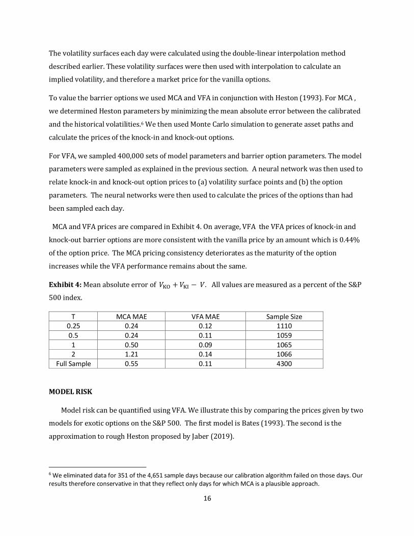
MCA and VFA prices are compared in Exhibit 4. On average, VFA the VFA prices of knock-in and

knock-out barrier options are more consistent with the vanilla price by an amount which is 0.44%

of the option price. The MCA pricing consistency deteriorates as the maturity of the option

increases while the VFA performance remains about the same.

Exhibit 4: Mean absolute error of 𝑉KO + 𝑉KI − 𝑉. All values are measured as a percent of the S&P

500 index.

T MCA MAE VFA MAE Sample Size 0.25 0.24 0.12 1110

0.5 0.24 0.11 1059

1 0.50 0.09 1065 2 1.21 0.14 1066

Full Sample 0.55 0.11 4300

MODEL RISK

Model risk can be quantified using VFA. We illustrate this by comparing the prices given by two

models for exotic options on the S&P 500. The first model is Bates (1993). The second is the

approximation to rough Heston proposed by Jaber (2019).

6 We eliminated data for 351 of the 4,651 sample days because our calibration algorithm failed on those days. Our results therefore conservative in that they reflect only days for which MCA is a plausible approach.

17

The steps used to produce results for each of the models and exotic options considered are as

follows:

(a) Model parameters are generated randomly as discussed in the previous section. For each

set of model parameters, a set of parameters describing the exotic option are also generated

randomly. For each of the resulting data sets, the standard points on the volatility surface

are calculated and the exotic option is valued.

(b) Data from step (a) are used to construct a neural network. The features are the volatility

surface points and the exotic option parameters while the target is the exotic option price.

(c) The neural network in (b) is used to price a panel of exotic options using historical data on

the asset of interest (the S&P 500 in our case)

The price differences when different models are used to price the same panel of exotic options

provide statistics to quantify model risk

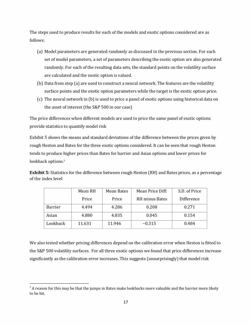
Exhibit 5 shows the means and standard deviations of the difference between the prices given by

rough Heston and Bates for the three exotic options considered. It can be seen that rough Heston

tends to produce higher prices than Bates for barrier and Asian options and lower prices for

lookback options.7

Exhibit 5: Statistics for the difference between rough Heston (RH) and Bates prices, as a percentage

of the index level

Mean RH

Price

Mean Bates

Price

Mean Price Diff:

RH minus Bates

S.D. of Price

Difference

Barrier 4.494 4.286 0.208 0.271

Asian 4.880 4.835 0.045 0.154

Lookback 11.631 11.946 −0.315 0.484

We also tested whether pricing differences depend on the calibration error when Heston is fitted to

the S&P 500 volatility surfaces. For all three exotic options we found that price differences increase

significantly as the calibration error increases. This suggests (unsurprisingly) that model risk

7 A reason for this may be that the jumps in Bates make lookbacks more valuable and the barrier more likely to be hit.

18

increases as the deviation of the volatility surface from the volatility surfaces given by models

commonly used increases.

CONCLUSIONS

In this paper, we have contrasted two approaches for valuing exotic options. One widely used

approach, MCA, involves fitting a model to the current volatility surface as closely as possible. The

other approach, VFA, uses the model in a different way. It relates points on the volatility surface to

the price and allows a neural network to learn which points on the volatility surface are most

relevant for valuing a particular exotic option. Tests show that VFA provides an interesting

alternative to local volatility models for analysts who are concerned that MCA leads to arbitrage

opportunities between exotic options and vanilla options.

References

Bates D. S. 1996. “Jumps and Stochastic Volatility: Exchange Rate Processes Implicit in

Deutschemark Options.” Review of Financial Studies 9 (1): 69-107.

Derman, E. and I. Kani. 1994. “Riding on a Smile.” Risk (February): 32-39.

Dupire B. 1994. “Pricing with a Smile.” Risk. (January):18-20.

El Euch O., J. Gatheral, and M. Rosenbaum. 2019. “Roughening Heston.” Risk (May): 84-89.

Federal Reserve System. 2011. “SR Letter 11-7: Supervisory Guidance on Model Risk Management.”

Washington, DC.

Ferguson R. and A. Green. 2018. “Deeply Learning Derivatives.” Working paper, arXiv: 1809.02233.

Gatheral J., T. Jaisson, M. Rosenbaum. 2018. “Volatility is Rough.” Quantitative Finance. 18 (6):933-

949.

Heston S. L. 1993. “A Closed Form Solution for Options with Stochastic Volatility with Applications

to Bond and Currency Options.” Review of Financial Studies. 6 (2): 327-343.

19

Horvath B., A. Muguruza, M. Tomas. 2021. “Deep Learning Volatility: A Deep Neural Network

Perspective on Pricing and Calibration in (Rough) Volatility Models.” Quantitative Finance. 21 (1):

11-27.

Hull, J. C. and A. White. 1997. “The Pricing of Options on Assets with Stochastic Volatility.” Journal of

Finance. 42 (2): 281-300.

Jaber E. A. 2019. “Lifting the Heston model.” Quantitative Finance. 19 (12): 1995-2013.

Liu S., A. Borovykh, L. A. Grzelak, C. W. Oosterlee. 2019. “A Neural Network-based Framework for

Financial Model Calibration. Journal of Mathematics in Industry.

9(9), https://doi.org/10.1186/s13362-019-0066-7.

Madan, D. B., P. P. Carr, and E. C. Chang. 1988. “The Variance-Gamma Process and Option Pricing.”

European Finance Review. 2: 79-105.

Merton R. C. 1976. “Option Pricing when Underlying Stock Returns are Discontinuous.” Journal of

Financial Economics. 3 (1-2): 125-144.

Ren, Y., D. Madan, and M. Q. Qian (2007), “Calibrating and Pricing with Enbedded Local Volatility

Models.” Risk. (September): 138-143.

Saporito, Y. F., X. Yang, and J. P. Zubelli. 2019. “The Calibration of Stochastic Local Volatility models:

An Inverse Problem Perspective.” Computers and Mathematics with Applications. 77 (12): 3054-

3067.

Sundararajan M., A. Taly, and Q. Yan. 2017. “Axiomatic Attributions for Deep Networks.”

Proceedings of 34th International Conference on Machine Learning: 3319-3328.

Vinh, N. X., J. Epps, and J. Bailey. 2010. “Information Theoretic Measures for Clusterings

Comparison: Variants, Properties, Normalization and Correction for Chance.” Journal of Machine

Learning Research. 11: 2837–2854.