deep learning for natural language...
TRANSCRIPT
Deep Learning for Natural LanguageProcessing
Sidharth MudgalApril 4, 2017

Table of contents
1. Intro
2. Word Vectors
3. Word2Vec
4. Char Level Word Embeddings
5. Application: Entity Matching
6. Conclusion
1

Intro

Intro
Deep Learning

Core Idea
• Given data that has hard to describe complex intrinsic structure• Important: DL usually works well only when data has unknownhidden structure. Not a silver bullet for all tasks
• Learn hierarchical representations of data points to perform atask
2

Typical flow
• Input representation• Hidden representations (higher level features)• Output prediction
3

Main Challenge
• Assisting the neural network to learn to create goodrepresentations
• How?• Encoding domain knowledge• Make training easier
• Improved optimization techniques• Better gradient flow
4
Model Engineering
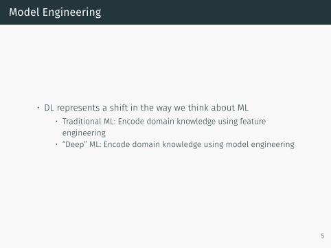
• DL represents a shift in the way we think about ML• Traditional ML: Encode domain knowledge using featureengineering
• “Deep” ML: Encode domain knowledge using model engineering
5

Intro
Natural Language Processing

What is NLP? (from Stanford CS224n)
6
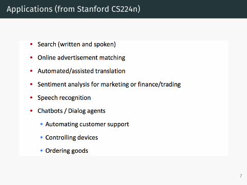
Applications (from Stanford CS224n)
7
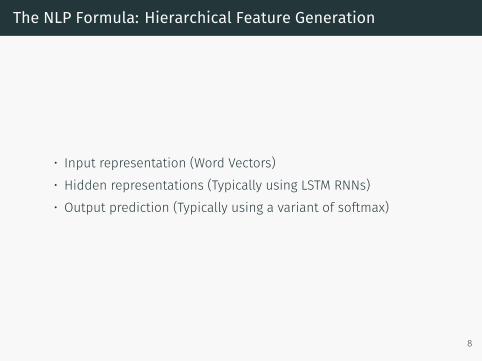
The NLP Formula: Hierarchical Feature Generation
• Input representation (Word Vectors)• Hidden representations (Typically using LSTM RNNs)• Output prediction (Typically using a variant of softmax)
8

Word Vectors

Word Vectors
Motivation

What do we want?
We want a representation of words that:
• Captures meaning• Is efficient
9

Past attempts to capture meaning of words - WordNet
10
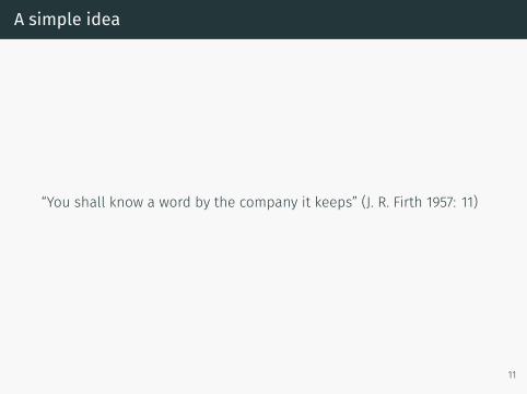
A simple idea
“You shall know a word by the company it keeps” (J. R. Firth 1957: 11)
11
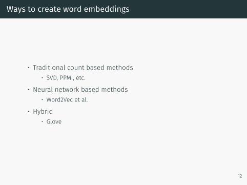
Ways to create word embeddings
• Traditional count based methods• SVD, PPMI, etc.
• Neural network based methods• Word2Vec et al.
• Hybrid• Glove
12

Word Vectors
Language Modeling

What is a Language Model?
• A probability distribution over sequences of wordsP(w1, · · · ,wm) =
∏mt=1 P(wt|wt−1, · · · ,w1)
• In practice, we only condition on the last M wordsP(w1, · · · ,wm) =
∏mt=1 P(wt|wt−1, · · · ,wt−M)
13
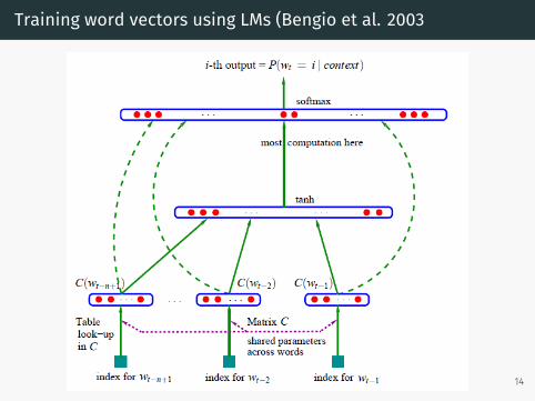
Training word vectors using LMs (Bengio et al. 2003
14

Word2Vec

Core Idea
• Parameterize words as vectors• Use an NN to predict nearby words
• Skip Gram• CBOW
• Hope that learned word vectors are semantically meaningful
15

Skip Gram Model
16
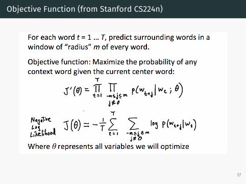
Objective Function (from Stanford CS224n)
17

How do we predict nearby words? (from Stanford CS224n)
18

Step by step (from Stanford CS224n)
19
The problem of Softmax
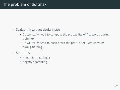
• Scalability wrt vocabulary size• Do we really need to compute the probability of ALL words duringtraining?
• Do we really need to push down the prob. of ALL wrong wordsduring training?
• Solutions:• Hierarchical Softmax• Negative sampling
20

The problem of Softmax
21
Hierarchical Softmax - Simple version
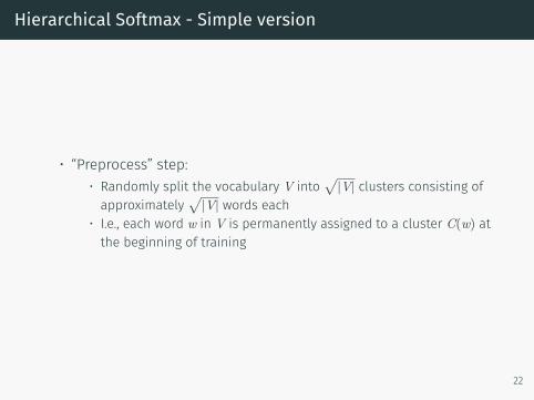
• “Preprocess” step:• Randomly split the vocabulary V into
√|V| clusters consisting of
approximately√
|V| words each• I.e., each word w in V is permanently assigned to a cluster C(w) atthe beginning of training
22
Hierarchical Softmax - Simple version
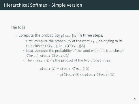
The Idea
• Compute the probability p(wt−1 |⃗ct) in three steps:• First, compute the probability of the word wt−1 belonging to itstrue cluster C(wt−1), i.e., p(C(wt−1)|⃗ct)
• Next, compute the probability of the word within its true clusterC(wt−1), p(wt−1|C(wt−1), c⃗t)
• Then, p(wt−1 |⃗ct) is the product of the two probabilities:
p(wt−1 |⃗ct) = p(wt−1,C(wt−1)|⃗ct)
= p(C(wt−1)|⃗ct)× p(wt−1|C(wt−1), c⃗t)
23

Hierarchical Softmax - Simple version
• Computing cluster probability p(C(wt−1)|⃗ct):• Use a regular softmax NN with
√|V| classes, 1 for each cluster.
24

Hierarchical Softmax - Simple version
• Computing word in cluster probability p(wt−1|C(wt−1), c⃗t):• To do so, each word cluster has a dedicated softmax NN withapproximately
√|V| classes, 1 for each word in the cluster.
25

Hierarchical Softmax
• Time complexity of simple version = O(√|V|)
• Can do much better (O(log |V|)) with more complex versions• Frequency based clustering of words• Brown clustering• etc...
26
Negative Sampling
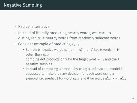
• Radical alternative• Instead of literally predicting nearby words, we learn todistinguish true nearby words from randomly selected words
• Consider example of predicting wt−1
• Sample k negative words n1t−1, · · · ,nk
t−1 ∈ V, i.e., k words in Vother than wt−1
• Compute dot products only for the target word wt−1 and the knegative samples
• Instead of computing a probability using a softmax, the model issupposed to make a binary decision for each word using asigmoid, i.e., predict 1 for word wt−1 and 0 for words n1
t−1, · · · ,nkt−1
27

Results
E.g.: France - Paris + Italy ≈ Rome
28
Drawbacks
• Learns word vectors independently for each word• Cannot estimate word embeddings of out-of-vocabulary (OOV)words
29
Char Level Word Embeddings
Core Idea
• Make use of fact that words are composed of characters• Parameterize characters as vectors• Compose char vectors to create word vectors
• Can use CNN or RNN
• Use an NN to predict nearby words• Hope that word vectors are semantically meaningful
30

The Word Embedding Network (WEN)
31
Step 1: Lookup Char Embeddings
• Same as word vector lookup layer
32
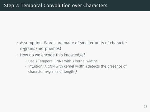
Step 2: Temporal Convolution over Characters
• Assumption: Words are made of smaller units of charactern-grams (morphemes)
• How do we encode this knowledge?• Use k Temporal CNNs with k kernel widths• Intuition: A CNN with kernel width j detects the presence ofcharacter n-grams of length j
33

Step 2: Temporal Convolution over Characters
• Example: Temporal convolution with kernel width = 3 and twofeature maps sensitive to 3-grams “mac” and “est”
34
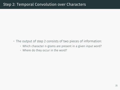
Step 2: Temporal Convolution over Characters
• The output of step 2 consists of two pieces of information:• Which character n-grams are present in a given input word?• Where do they occur in the word?
35

Step 3: Max-Pooling
• For each feature map in each CNN, output only the maximumactivation
• Intuition: Get rid of the position information of charactern-grams
• This yeilds a fixed dimensional vector
36
Step 4: Fully Connected Layers
• 3-layer “highway network”• Intuition: Compose a word vector using information about whichcharacter n-grams are present in the word
37
Step 4: Highway NN Layer Details
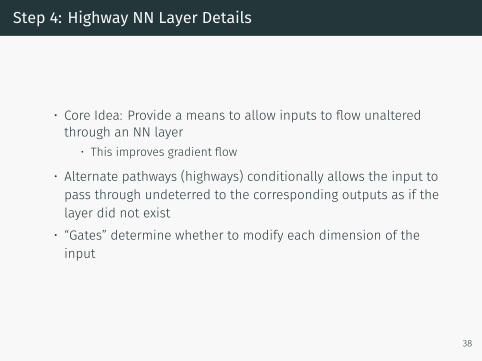
• Core Idea: Provide a means to allow inputs to flow unalteredthrough an NN layer
• This improves gradient flow
• Alternate pathways (highways) conditionally allows the input topass through undeterred to the corresponding outputs as if thelayer did not exist
• “Gates” determine whether to modify each dimension of theinput
38

Step 4: Highway NN Layer Details
39

Step 4: Highway NN Layer Details
Given an input vector q⃗, the output of the nth highway layer withinput x⃗n and output y⃗n is computed as follows:
x⃗n =
{q⃗, if n = 1,y⃗n−1, if n > 1
H(⃗xn) = W⃗(H)n x⃗n + b⃗(H)
n
T(⃗xn) = W⃗(T)n x⃗n + b⃗(T)
n
y⃗n = H(⃗xn)⊙ T(⃗xn) + x⃗n ⊙ (1 − T(⃗xn))
Here H applies an affine transformation to x⃗n and T acts as the gatedeciding which inputs should be transformed and by how much.
40
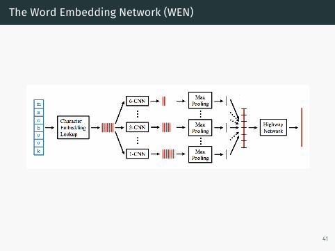
The Word Embedding Network (WEN)
41

Training the Word Embedding Network
• How can we train this model to produce good wordembeddings?
• Train it as part of a recurrent neural language model
42

Training
43

Results
44

Application: Entity Matching

The Task
• Given text descriptions of two entities, determine if they refer tothe same real world entity
• Binary classification problem
45

The Task
• Typical approach: Information Extraction (IE)• Followed by training a traditional classifier: SVM, Random Forestetc.
• Proposed alternate approach: Neural Entity Matching Model(Nemo)
• Use deep learning to perform this end to end• Train a single model to perform extraction and entity matching
46

Nemo Overview
47
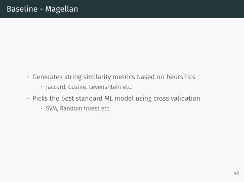
Baseline - Magellan
• Generates string similarity metrics based on heursitics• Jaccard, Cosine, Levenshtein etc.
• Picks the best standard ML model using cross validation• SVM, Random forest etc.
48
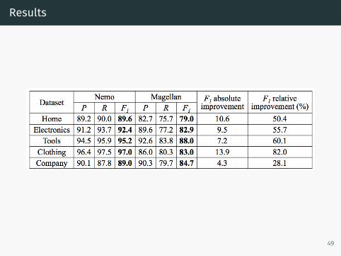
Results
49

Results - Extensive extraction
50

Understanding the model
• Compute first order saliency scores for word embeddings• Essentially the derivative of word embeddings wrt the output ofthe model
• Measure of sensitivity
51

Understanding the model
Example:
• Assume we have an entity pair (e1, e2)
• We want to compute the saliency of the tth word in e1
• If yL represents the score that Nemo assigns to the correct labelL (match or mismatch) for the pair, x⃗t represents Nemo’s inputunits for the tth word and w⃗t is the word embedding of the tthword in e1, then the saliency s of the word is calculated as
s =∥∥∥∥∂yL∂x⃗t
|x⃗t=w⃗t
∥∥∥∥
52

Saliency Visualization
53
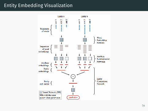
Entity Embedding Visualization
54
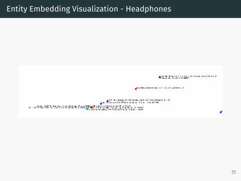
Entity Embedding Visualization - Headphones
55

Entity Embedding Visualization - Cables
56
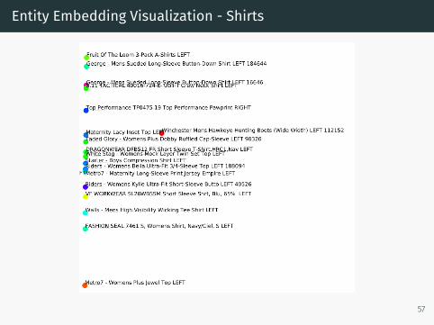
Entity Embedding Visualization - Shirts
57

Entity Embedding Visualization - Bags
58

Entity Embedding Visualization - Desks
59

Conclusion

Deep Learning: An incredibly promising tool
• Has produced breakthroughs in several domains• But has a lot of open problems
• Large quantities of labeled data• Huge number of parameters• Optimization challenges
60