Deep Learning for Physics DiscoveryWinter 2021

Wai Tong Chungwtchung@stanford.edu

Danyal Mohaddes Khorassanidanmohad@stanford.edu

Jacob Roy Westjrwest@stanford.edu

AbstractA variational autoencoder is employed to gain insights into two physical systems: a particle settling under gravity in a viscousfluid, and a chemical reactor. The network architecture allows the interpretation of neuron activations in the latent layer in termsof physical parameters governing system behavior. The network takes as input a set of observations, a question regarding thestate of nature under particular conditions, and an answer describing the state of nature under said conditions. The architecturewas shown to yield accurate, interpretable results in both physical systems of interest, correctly discerning the parametersgoverning the physical systems and storing them in the latent neuron activations, and providing additional physical insight intothe systems at hand.

1 Introduction

Figure 1: Example data for the particle motionproblem.

From Archimedes to Ibn-Khwarazmi to Newton, physicists have always relied upon a combina-tion of observation of nature and deductive reasoning to discover the laws of nature. Physicistsgenerally have access to a set of observations tou, often from experimentation, that are indica-tive of a deterministic relationship among variables of interest. The objective of the physicistis then to determine the function f which represents the deterministic mapping between sup-posed physical conditions termed questions q to particular states of nature termed answers a,i.e. f : q Ñ a. Crucially, once f has been found, its structure is then analyzed, for it is theinterpretation of this structure that yields insight into the inner workings of natural laws. Thatf be merely an accurate mapping from q to a is a necessary condition for meaningful physicalanalysis, but it is not sufficient.

Traditional neural network architectures used in deep learning are akin to “black-boxes”, in thatwith a sufficiently large observational data set tou they can be trained to offer an accurate map-ping function f : q Ñ a, but offer little insight. This is because the activations of hidden layersin a deep neural network, though containing the information necessary to achieve the afore-mentioned accurate mapping, represent a high-dimensional non-linear parameter space. Thisis in stark contrast to traditional physics-based models, where each model parameter representsspecific physical mechanisms or their interaction. Consequently, physics-based models have ahigh degree of interpretability. Nevertheless, developments in interpretable deep learning havesuggested a promising path towards automatic scientific discovery.

A deep learning model called Scinet, which incorporates a variational autoencoder [1], wasshown to automatically extract physical laws from several fundamental physics problems.When employed to predict planetary motion from raw geocentric planetary angles, the model’sinterpretable latent activations were shown to transform planetary angles from geocentric toheliocentric coordinates, thus demonstrating the network’s ability to automatically recover necessary intermediate steps within complex calcula-tions from unprocessed observations. To this end, we have applied the SciNet network architecture to extract interpretable scientific insight fromcanonical problems in fluid dynamics and combustion.

We will discuss the details of the network architecture in Sec. 4. Briefly, the inputs to the encoder network are a set of observations |tou| “ No,where each observation is a vector in Rn of observed variables rv1, v2, ..., vns. The data input to the decoder network is a question q, which is avariable which defines the condition under which the state of nature is to be inquired, with other inputs coming from other parts of the network.The output of the decoder network is the answer a, which is the state of nature under the conditions stipulated by the question q.

2 Related workThere has been growing interest in the use of what can be broadly considered “data-driven” techniques for the advancement of the field ofphysics, as opposed to the traditional “pen-and-paper” methodology. A conservative approach (conservative in the sense of similarity withtraditional physical analysis) was taken by Floryan and Graham [2]. The authors employ a spectral decomposition technique and combined it

CS230: Deep Learning, Winter 2018, Stanford University, CA. (LateX template borrowed from NIPS 2017.)

Encoder Decoder # Training samples # Dev samples # Test samples[500,100] [100,100] 200,000 10,000 10,000

Table 1: Scinet architecture and dataset breakdown used for the particle motion sub-problem.

Encoder Decoder # Training samples # Dev samples # Test samples[500,100] [100,100] 1500 250 250

Table 2: Scinet architecture and dataset breakdown used for the chemistry sub-problem.

with a data-driven approach to extract the persistent features of physical systems across large ranges of time and scale. A more radical approachwas taken by Wu and Tegmark [3], who aimed to develop an “AI physicist”. They combine a number of ideas from both artificial intelligence andclassical physics to develop an “agent” whose purpose is to learn new theories of physics and attempt to unify them when presented with data in anunsupervised setting. The authors successfully demonstrate their model by applying their agent to accurately predict particle motion in domainsgoverned by a harmonic potential field, a gravitational field and an electromagnetic field. An approach that lies between the two aforementionedextremes is that proposed by Iten et al. [1], upon which this project is based. The authors refrain from creating an agent-based automatic physicsdiscovery system, but instead use an encoder-decoder architecture where a latent neuron layer is designed to capture physical insights in afashion inspired by the process physicists employ in traditional analysis. The authors apply their methodology to various physical systems anddemonstrate that their architecture is well-suited to capturing key insights into system behavior and stores them in the activations of the latentneurons, such as the number of parameters necessary to accurately describe system dynamics, and even coordinate transformations.

3 Dataset and Features3.1 Particle Motion

Figure 2: Architecture of Scinet (taken from [1],Figure 1b)

The motion of a particle in a viscous fluid is typically described by ODEs relating the forceson the particle to its velocity [4]. These forces are parametrized by properties of the fluid andparticle, and its velocity, which may not be constant in time. A very simple model for particlemotion is described by two constant parameters, the Stokes number, St which describes thedrag force, and the Froude number Fr, which describes the gravitational force. Given a particleinitially at rest at position x “ 0, its future position at time t is given by

xptq “ St2Frr1´1

Stt´ expp´t{Stqs (1)

Fr is sampled uniformly from the range r0, 5s and St is sampled logarithmically from the ranger0.01, 100s to synthetically generate training data for this problem. The observations are a setof 50 xptq, uniformly spaced in the range t “ r0, 1s, evaluating equation 1. The “question” isa time randomly chosen in the range tq “ r0, 2s, and the “answer” is the position xptqq. Thisforces the decoder to extrapolate to a time where it does not have direct observations. Exampleobservations, questions, and answers for two different parameter combinations are shown inFigure 1.

This problem setup is very similar to the pendulum problem studied in [1], and so the same architecture is used. The architecture details anddataset size are given in Table 1.

3.2 ChemistryWe apply the chemistry package Cantera [5] to calculate the formation of CO2 and water from methane and oxygen with a single step chemistryin an isothermal zero-dimensional reactor:

CH4 ` 2O2 ÝÑ CO2 ` 2H2O (2)drCO2s

dt“ kf pT qrCH4srO2s

2 (3)

where the forward rate constant kf is a function of temperature and the brackets [φ] refer to the concentration of scalar φ. 2000 samples of dataare generated from range T “ r1000, 3000s K.

The “observation” data consists of CO2 mass fraction YCO2 as a function of time before time t “ r0, 12.5s µs, with a timestep of 0.5 µs. The“answer” consists of YCO2 at t “ r0, 25s µs, and the “question” consists of 3 neurons corresponding to time, YCH4, and YO2. The training detailsfor Scinet are provided in Table 2.

4 MethodsWe employ the Scinet architecture in this study, shown in Figure 2. Scinet trains an encoder on observation data o, which condenses the inputto a much smaller latent representation. Then, instead of reconstructing the input directly, the latent representation and question q are fed into adecoder network to provide an answer a. Users provide triples of po, q, aq as training data. This structure mimics the scientific task of observingexperiments, creating a model, and assessing the accuracy of the model predictions.

2

Training phase Batch size Learning rate β # Epochs1 512 10´3 10´3 1,0002 1024 10´4 10´3 5003 1024 10´5 10´3 500

Table 3: Hyperparameters used to train Scinet on the particle motion sub-problem.

Since the goal of this network is a model which is both descriptive and interpretable, there are two parts to the Scinet loss function, which is basedon the β-VAE cost function [6]:

Cost “1

Nbatch

Nbatchÿ

i“1

˜

||ai ´ ai||2 ´β

2

ˆNlatentÿ

j“1

`

logpσ2ijq ´ µ

2ij ´ σ

2ij ´ 1

˘

˙

¸

(4)

where the first term represents the distance between the correct and predicted answers, a and a. The second term approximates the KL divergenceunder certain assumptions detailed in the supplemental material of [1]. µij and σij represent the mean and standard deviation of the latent activa-tion distribution for latent neuron j on example i. β is a hyperparameter which controls the relative importance of the two objectives. Individualterms are summed over Nbatch examples in a batch. Depending on the physical problem addressed, Scinet uses different hyperparameters, butgenerally speaking, it uses 2 fully connected layers each in the encoder and decoder. The Adam optimizer is used, with Op100, 000q examples,5% of which are used in the dev set.

5 Results and Discussion5.1 Particle Motion

Figure 3: Training and dev losses during train-ing of Scinet with 2 latent neurons, and the ab-solute value of their difference.

The training hyperparameters are largely adapted from the “pendulum” problem in [1], but alsousing multiple phases as in their “heliocentric” problem. The parameters used during trainingfor all of the following results are shown in Table 3. Decreasing the learning rate and increasingthe batch size through multiple phases of training was helpful in reducing the large oscillationsin the loss function, which can be seen in Fig. 3. The difference between training and dev lossesis consistently about 3 orders of magnitude smaller than the losses themselves, which indicatesthat overfitting is not a problem.

A key goal of Scinet is to correctly determine the minimum number of parameters needed tofully describe a dataset, where each parameter is represented by the activation of a differentlatent neuron. To assess the network’s performance, we used the same procedure to train net-works with 1´ 4 latent neurons. The components of the loss function (reconstruction loss andKL divergence loss) are plotted against the number of latent neurons in Figure 4. This showsa substantial improvement in reconstruction loss going from 1 to 2 neurons, and then no addedbenefit. The KL divergence loss increases slightly when using more than 1 neuron, but this issomewhat expected as there are more latent neurons to sum over. The fact that the KL loss doesnot increase beyond 2 neurons indicates that the additional neurons are not active.

When the latent space is too small, the network is forced to learn a representation which istoo compact to represent all the characteristics of the data. When the latent space is too large,Scinet should set those unecssary activations to zero. This behavior is demonstrated in Figure5, which shows the latent activations on test data for networks with 1´3 latent neurons, plottedagainst the input parameters. A few observations can be made:

• With more than 1 neuron, the ordering of the latent activations is probably a result of random initialization. Nothing was done to ensuresimilarity among the first neurons.

• The contours of the first activation are very similar across cases. However, with the 2 neuron network, the activation appears to bemultiplied by ´1. This is probably also a result of random initialization, and it indicates that the learned parameters could be simpletransformations of the true parameters.

• The fact that the 1 neuron network has learned essentially the same representation as the first neurons of the other networks suggests thatScinet could be used to identify useful reduced models for physical phenomena, which have a more limited range of applicability.

Figure 5 can only be made when the input parameters are known. However, it suggests that for networks with several active latent neurons, theextracted feature can be understood by dropping out different neurons and assessing the kinds of errors the network makes. This may help suggestto the scientist the kinds of patterns the network has been able to find.

5.2 ChemistryTraining Scinet for the chemistry problem adopted a similar approach to the particle problem in section Section 5.1, with hyperparameters shownin Table 4. Since only 2000 datapoints are used for train, dev, and test sets, a smaller batch size has been adopted. Training is found to haveconverged around 200 epochs as shown in Fig. 6b. The difference between training and dev losses is consistently about 2 orders of magnitudesmaller than the losses themselves, which indicates that overfitting is not a problem. Additionally, the predictions from Scinet are found to be ingood agreement with the correponding true CO2 mass fractions as shown in Fig. 6a.

3

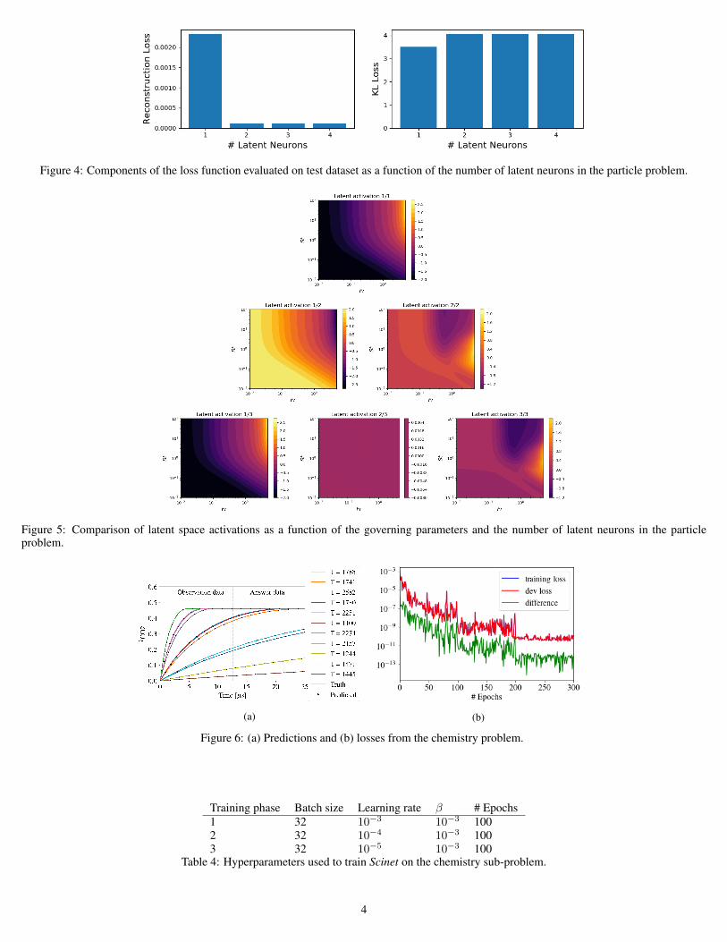
Figure 4: Components of the loss function evaluated on test dataset as a function of the number of latent neurons in the particle problem.

Figure 5: Comparison of latent space activations as a function of the governing parameters and the number of latent neurons in the particleproblem.

(a) (b)

Figure 6: (a) Predictions and (b) losses from the chemistry problem.

Training phase Batch size Learning rate β # Epochs1 32 10´3 10´3 1002 32 10´4 10´3 1003 32 10´5 10´3 100

Table 4: Hyperparameters used to train Scinet on the chemistry sub-problem.

4

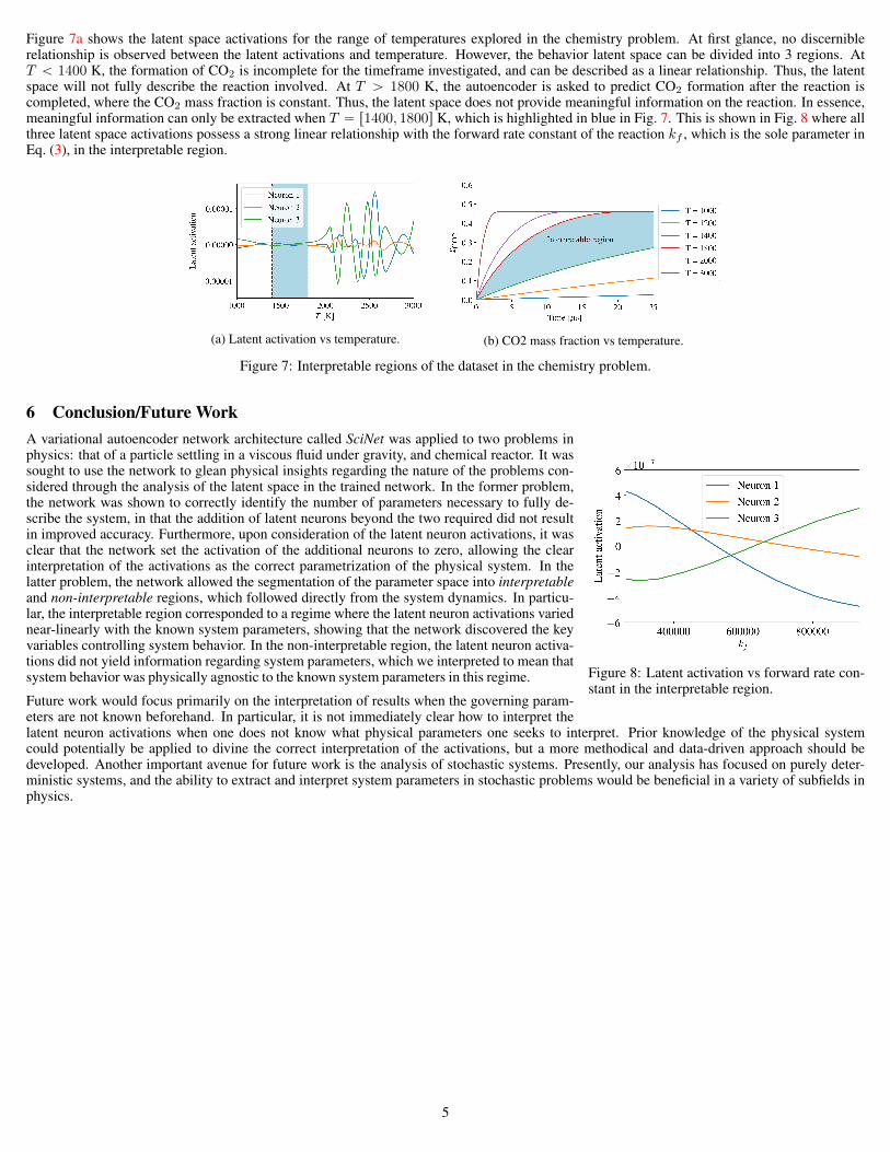
Figure 7a shows the latent space activations for the range of temperatures explored in the chemistry problem. At first glance, no discerniblerelationship is observed between the latent activations and temperature. However, the behavior latent space can be divided into 3 regions. AtT ă 1400 K, the formation of CO2 is incomplete for the timeframe investigated, and can be described as a linear relationship. Thus, the latentspace will not fully describe the reaction involved. At T ą 1800 K, the autoencoder is asked to predict CO2 formation after the reaction iscompleted, where the CO2 mass fraction is constant. Thus, the latent space does not provide meaningful information on the reaction. In essence,meaningful information can only be extracted when T “ r1400, 1800s K, which is highlighted in blue in Fig. 7. This is shown in Fig. 8 where allthree latent space activations possess a strong linear relationship with the forward rate constant of the reaction kf , which is the sole parameter inEq. (3), in the interpretable region.

(a) Latent activation vs temperature. (b) CO2 mass fraction vs temperature.

Figure 7: Interpretable regions of the dataset in the chemistry problem.

6 Conclusion/Future Work

Figure 8: Latent activation vs forward rate con-stant in the interpretable region.

A variational autoencoder network architecture called SciNet was applied to two problems inphysics: that of a particle settling in a viscous fluid under gravity, and chemical reactor. It wassought to use the network to glean physical insights regarding the nature of the problems con-sidered through the analysis of the latent space in the trained network. In the former problem,the network was shown to correctly identify the number of parameters necessary to fully de-scribe the system, in that the addition of latent neurons beyond the two required did not resultin improved accuracy. Furthermore, upon consideration of the latent neuron activations, it wasclear that the network set the activation of the additional neurons to zero, allowing the clearinterpretation of the activations as the correct parametrization of the physical system. In thelatter problem, the network allowed the segmentation of the parameter space into interpretableand non-interpretable regions, which followed directly from the system dynamics. In particu-lar, the interpretable region corresponded to a regime where the latent neuron activations variednear-linearly with the known system parameters, showing that the network discovered the keyvariables controlling system behavior. In the non-interpretable region, the latent neuron activa-tions did not yield information regarding system parameters, which we interpreted to mean thatsystem behavior was physically agnostic to the known system parameters in this regime.

Future work would focus primarily on the interpretation of results when the governing param-eters are not known beforehand. In particular, it is not immediately clear how to interpret thelatent neuron activations when one does not know what physical parameters one seeks to interpret. Prior knowledge of the physical systemcould potentially be applied to divine the correct interpretation of the activations, but a more methodical and data-driven approach should bedeveloped. Another important avenue for future work is the analysis of stochastic systems. Presently, our analysis has focused on purely deter-ministic systems, and the ability to extract and interpret system parameters in stochastic problems would be beneficial in a variety of subfields inphysics.

5

7 ContributionsWTC developed the chemistry SciNet application. DMK developed a thermodynamics SciNet application (discussed in the proposal and mile-stone) and contributed to the dataset generation for the chemistry application. JRW developed the particle motion SciNet application. All authorscontributed to analysis and report writing.

8 References[1] R. Iten, T. Metger, H. Wilming, L. del Rio, and R. Renner, “Discovering physical concepts with neural networks,” Phys. Rev. Lett., vol. 124,

p. 010508, Jan 2020.

[2] D. Floryan and M. D. Graham, “Discovering multiscale and self-similar structure with data-driven wavelets,” Proceedings of the NationalAcademy of Sciences, vol. 118, no. 1, 2021.

[3] T. Wu and M. Tegmark, “Toward an ai physicist for unsupervised learning.(2018),” arXiv preprint arXiv:1810.10525, 1810.

[4] M. R. Maxey and J. J. Riley, “Equation of motion for a small rigid sphere in a nonuniform flow,” The Physics of Fluids, vol. 26, no. 4,pp. 883–889, 1983.

[5] D. G. Goodwin, R. L. Speth, H. K. Moffat, and B. W. Weber, “Cantera: An object-oriented software toolkit for chemical kinetics, thermody-namics, and transport processes,” 2018. https://www.cantera.org.

[6] I. Higgins, L. Matthey, A. Pal, C. Burgess, X. Glorot, M. Botvinick, S. Mohamed, and A. Lerchner, “beta-vae: Learning basic visual conceptswith a constrained variational framework,” 2016.

6