deep learning - stm 6
TRANSCRIPT
Deep Learning for Computer Vision
Igor Trajkovski
[email protected] twitter.com/mkrobot
facebook.com/mkrobot
SkopjeTechMeetup 29.9.2016
Slides from Andrej Karpathy, Yann LeCun & Geoffrey Hinton

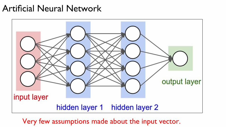
Artificial Neural Network
Artificial Neural Network
Very few assumptions made about the input vector.

In many real-world applications input vectors have structure.
Spectrograms
Images Text

Convolutional Neural Networks:A pinch of history

Hubel & Wiesel,1959RECEPTIVE FIELDS OF SINGLE NEURONES INTHE CAT'S STRIATE CORTEX
1962RECEPTIVE FIELDS, BINOCULAR INTERACTIONAND FUNCTIONAL ARCHITECTURE INTHE CAT'S VISUAL CORTEX
https://www.youtube.com/watch?v=8VdFf3egwfg
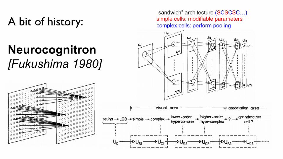
A bit of history: Neurocognitron [Fukushima 1980]
“sandwich” architecture (SCSCSC…) simple cells: modifiable parameters complex cells: perform pooling
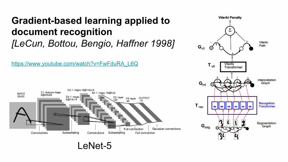
Gradient-based learning applied to document recognition [LeCun, Bottou, Bengio, Haffner 1998]
LeNet-5
https://www.youtube.com/watch?v=FwFduRA_L6Q
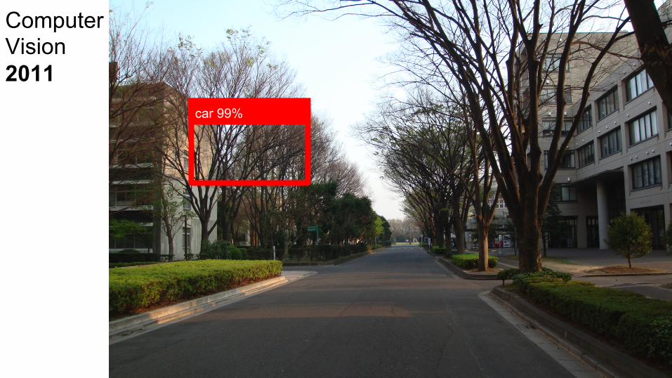
car 99%
Computer Vision 2011

Computer Vision 2011
+ code complexity :(
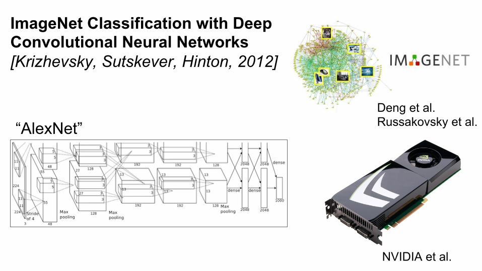
ImageNet Classification with Deep Convolutional Neural Networks [Krizhevsky, Sutskever, Hinton, 2012]
“AlexNet” Deng et al. Russakovsky et al.
NVIDIA et al.
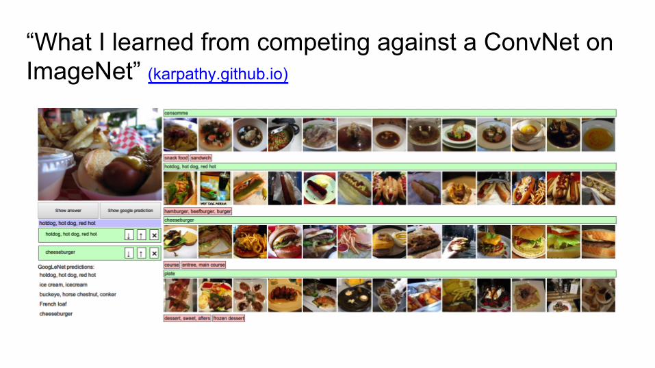
“What I learned from competing against a ConvNet on ImageNet” (karpathy.github.io)

“What I learned from competing against a ConvNet on ImageNet” (karpathy.github.io)
TLDR: Human accuracy is somewhere 2-5%. (depending on how much training or how little life you have)
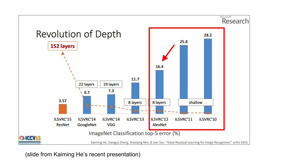
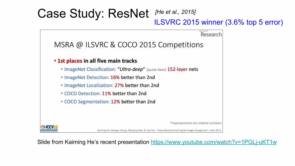
(slide from Kaiming He’s recent presentation)

[224x224x3]
f 1000 numbers, indicating class scores
Feature Extraction
vector describing various image statistics
[224x224x3]
f 1000 numbers, indicating class scores
training
training
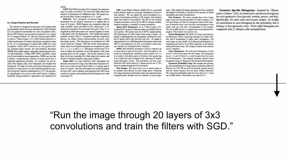
“Run the image through 20 layers of 3x3 convolutions and train the filters with SGD.”

Convolutional Neural Networks

[224x224x3]
f 1000 numbers, indicating class scores
training
Only two basic operations are involved throughout: 1. Dot products w.x 2. Max operations parameters
(~10M of them)
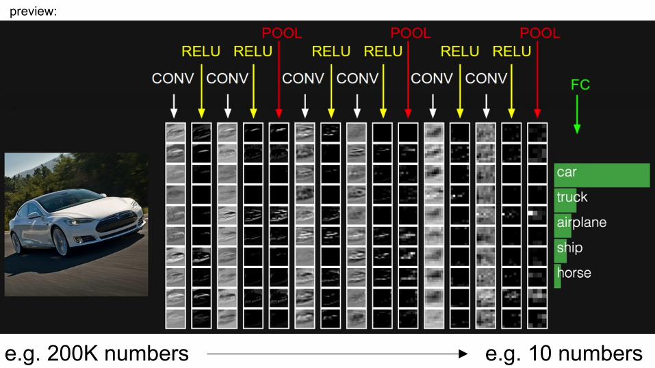
preview:
e.g. 200K numbers e.g. 10 numbers
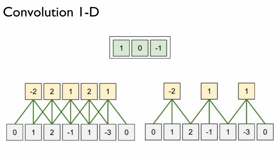
Convolution 1-D
1 -1 -1-1 1 -1-1 -1 1
-1 -1 -1 -1 -1 -1 -1 -1 -1-1 1 -1 -1 -1 -1 -1 1 -1-1 -1 1 -1 -1 -1 1 -1 -1-1 -1 -1 1 -1 1 -1 -1 -1-1 -1 -1 -1 1 -1 -1 -1 -1-1 -1 -1 1 -1 1 -1 -1 -1-1 -1 1 -1 -1 -1 1 -1 -1-1 1 -1 -1 -1 -1 -1 1 -1-1 -1 -1 -1 -1 -1 -1 -1 -1
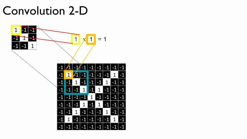
Convolution 2-D

11 -1 -1-1 1 -1-1 -1 1
-1 -1 -1 -1 -1 -1 -1 -1 -1-1 1 -1 -1 -1 -1 -1 1 -1-1 -1 1 -1 -1 -1 1 -1 -1-1 -1 -1 1 -1 1 -1 -1 -1-1 -1 -1 -1 1 -1 -1 -1 -1-1 -1 -1 1 -1 1 -1 -1 -1-1 -1 1 -1 -1 -1 1 -1 -1-1 1 -1 -1 -1 -1 -1 1 -1-1 -1 -1 -1 -1 -1 -1 -1 -1
Convolution 2-D

1 11 -1 -1-1 1 -1-1 -1 1
-1 -1 -1 -1 -1 -1 -1 -1 -1-1 1 -1 -1 -1 -1 -1 1 -1-1 -1 1 -1 -1 -1 1 -1 -1-1 -1 -1 1 -1 1 -1 -1 -1-1 -1 -1 -1 1 -1 -1 -1 -1-1 -1 -1 1 -1 1 -1 -1 -1-1 -1 1 -1 -1 -1 1 -1 -1-1 1 -1 -1 -1 -1 -1 1 -1-1 -1 -1 -1 -1 -1 -1 -1 -1
Convolution 2-D

1 1 11 -1 -1-1 1 -1-1 -1 1
-1 -1 -1 -1 -1 -1 -1 -1 -1-1 1 -1 -1 -1 -1 -1 1 -1-1 -1 1 -1 -1 -1 1 -1 -1-1 -1 -1 1 -1 1 -1 -1 -1-1 -1 -1 -1 1 -1 -1 -1 -1-1 -1 -1 1 -1 1 -1 -1 -1-1 -1 1 -1 -1 -1 1 -1 -1-1 1 -1 -1 -1 -1 -1 1 -1-1 -1 -1 -1 -1 -1 -1 -1 -1
Convolution 2-D

1 1 11
1 -1 -1-1 1 -1-1 -1 1
-1 -1 -1 -1 -1 -1 -1 -1 -1-1 1 -1 -1 -1 -1 -1 1 -1-1 -1 1 -1 -1 -1 1 -1 -1-1 -1 -1 1 -1 1 -1 -1 -1-1 -1 -1 -1 1 -1 -1 -1 -1-1 -1 -1 1 -1 1 -1 -1 -1-1 -1 1 -1 -1 -1 1 -1 -1-1 1 -1 -1 -1 -1 -1 1 -1-1 -1 -1 -1 -1 -1 -1 -1 -1
Convolution 2-D

1 1 11 1
1 -1 -1-1 1 -1-1 -1 1
-1 -1 -1 -1 -1 -1 -1 -1 -1-1 1 -1 -1 -1 -1 -1 1 -1-1 -1 1 -1 -1 -1 1 -1 -1-1 -1 -1 1 -1 1 -1 -1 -1-1 -1 -1 -1 1 -1 -1 -1 -1-1 -1 -1 1 -1 1 -1 -1 -1-1 -1 1 -1 -1 -1 1 -1 -1-1 1 -1 -1 -1 -1 -1 1 -1-1 -1 -1 -1 -1 -1 -1 -1 -1
Convolution 2-D

1 1 11 1 1
1 -1 -1-1 1 -1-1 -1 1
-1 -1 -1 -1 -1 -1 -1 -1 -1-1 1 -1 -1 -1 -1 -1 1 -1-1 -1 1 -1 -1 -1 1 -1 -1-1 -1 -1 1 -1 1 -1 -1 -1-1 -1 -1 -1 1 -1 -1 -1 -1-1 -1 -1 1 -1 1 -1 -1 -1-1 -1 1 -1 -1 -1 1 -1 -1-1 1 -1 -1 -1 -1 -1 1 -1-1 -1 -1 -1 -1 -1 -1 -1 -1
Convolution 2-D
1 1 11 1 11
1 -1 -1-1 1 -1-1 -1 1
-1 -1 -1 -1 -1 -1 -1 -1 -1-1 1 -1 -1 -1 -1 -1 1 -1-1 -1 1 -1 -1 -1 1 -1 -1-1 -1 -1 1 -1 1 -1 -1 -1-1 -1 -1 -1 1 -1 -1 -1 -1-1 -1 -1 1 -1 1 -1 -1 -1-1 -1 1 -1 -1 -1 1 -1 -1-1 1 -1 -1 -1 -1 -1 1 -1-1 -1 -1 -1 -1 -1 -1 -1 -1
Convolution 2-D
1 1 11 1 11 1
1 -1 -1-1 1 -1-1 -1 1
-1 -1 -1 -1 -1 -1 -1 -1 -1-1 1 -1 -1 -1 -1 -1 1 -1-1 -1 1 -1 -1 -1 1 -1 -1-1 -1 -1 1 -1 1 -1 -1 -1-1 -1 -1 -1 1 -1 -1 -1 -1-1 -1 -1 1 -1 1 -1 -1 -1-1 -1 1 -1 -1 -1 1 -1 -1-1 1 -1 -1 -1 -1 -1 1 -1-1 -1 -1 -1 -1 -1 -1 -1 -1
Convolution 2-D

1 1 11 1 11 1 1
1 -1 -1-1 1 -1-1 -1 1
-1 -1 -1 -1 -1 -1 -1 -1 -1-1 1 -1 -1 -1 -1 -1 1 -1-1 -1 1 -1 -1 -1 1 -1 -1-1 -1 -1 1 -1 1 -1 -1 -1-1 -1 -1 -1 1 -1 -1 -1 -1-1 -1 -1 1 -1 1 -1 -1 -1-1 -1 1 -1 -1 -1 1 -1 -1-1 1 -1 -1 -1 -1 -1 1 -1-1 -1 -1 -1 -1 -1 -1 -1 -1
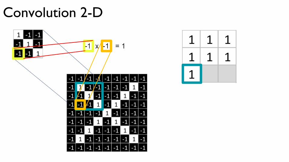
Convolution 2-D
1
1 1 11 1 11 1 1
1 -1 -1-1 1 -1-1 -1 1
-1 -1 -1 -1 -1 -1 -1 -1 -1-1 1 -1 -1 -1 -1 -1 1 -1-1 -1 1 -1 -1 -1 1 -1 -1-1 -1 -1 1 -1 1 -1 -1 -1-1 -1 -1 -1 1 -1 -1 -1 -1-1 -1 -1 1 -1 1 -1 -1 -1-1 -1 1 -1 -1 -1 1 -1 -1-1 1 -1 -1 -1 -1 -1 1 -1-1 -1 -1 -1 -1 -1 -1 -1 -1
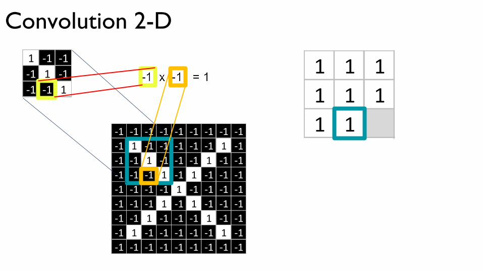
Convolution 2-D

11 -1 -1-1 1 -1-1 -1 1
-1 -1 -1 -1 -1 -1 -1 -1 -1-1 1 -1 -1 -1 -1 -1 1 -1-1 -1 1 -1 -1 -1 1 -1 -1-1 -1 -1 1 -1 1 -1 -1 -1-1 -1 -1 -1 1 -1 -1 -1 -1-1 -1 -1 1 -1 1 -1 -1 -1-1 -1 1 -1 -1 -1 1 -1 -1-1 1 -1 -1 -1 -1 -1 1 -1-1 -1 -1 -1 -1 -1 -1 -1 -1
Convolution 2-D

1 1 -11 -1 -1-1 1 -1-1 -1 1
-1 -1 -1 -1 -1 -1 -1 -1 -1-1 1 -1 -1 -1 -1 -1 1 -1-1 -1 1 -1 -1 -1 1 -1 -1-1 -1 -1 1 -1 1 -1 -1 -1-1 -1 -1 -1 1 -1 -1 -1 -1-1 -1 -1 1 -1 1 -1 -1 -1-1 -1 1 -1 -1 -1 1 -1 -1-1 1 -1 -1 -1 -1 -1 1 -1-1 -1 -1 -1 -1 -1 -1 -1 -1
Convolution 2-D

1 1 -11 1 1-1 1 1
1 -1 -1-1 1 -1-1 -1 1
-1 -1 -1 -1 -1 -1 -1 -1 -1-1 1 -1 -1 -1 -1 -1 1 -1-1 -1 1 -1 -1 -1 1 -1 -1-1 -1 -1 1 -1 1 -1 -1 -1-1 -1 -1 -1 1 -1 -1 -1 -1-1 -1 -1 1 -1 1 -1 -1 -1-1 -1 1 -1 -1 -1 1 -1 -1-1 1 -1 -1 -1 -1 -1 1 -1-1 -1 -1 -1 -1 -1 -1 -1 -1
Convolution 2-D
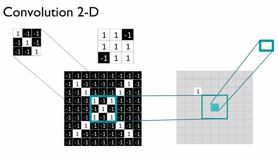
1
1 -1 -1-1 1 -1-1 -1 1
-1 -1 -1 -1 -1 -1 -1 -1 -1-1 1 -1 -1 -1 -1 -1 1 -1-1 -1 1 -1 -1 -1 1 -1 -1-1 -1 -1 1 -1 1 -1 -1 -1-1 -1 -1 -1 1 -1 -1 -1 -1-1 -1 -1 1 -1 1 -1 -1 -1-1 -1 1 -1 -1 -1 1 -1 -1-1 1 -1 -1 -1 -1 -1 1 -1-1 -1 -1 -1 -1 -1 -1 -1 -1
1 1 -11 1 1-1 1 1
55
1 1 -11 1 1-1 1 1
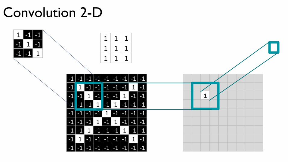
Convolution 2-D
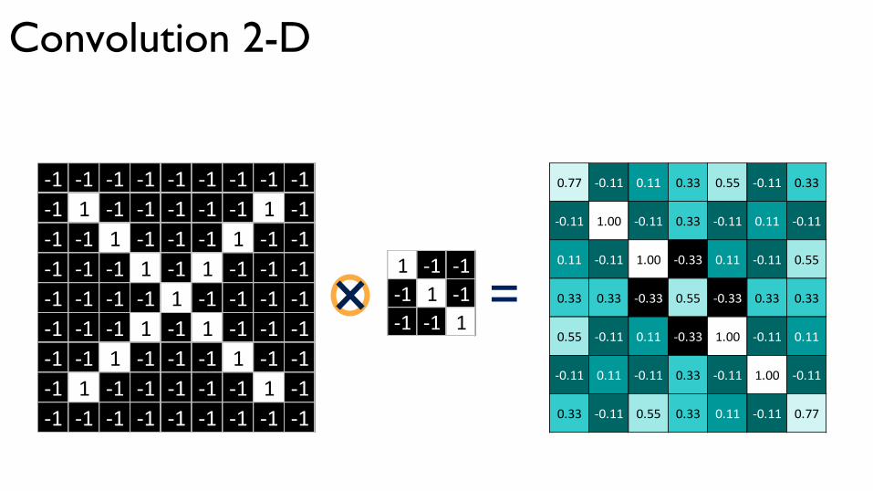
1 -1 -1-1 1 -1-1 -1 1
-1 -1 -1 -1 -1 -1 -1 -1 -1-1 1 -1 -1 -1 -1 -1 1 -1-1 -1 1 -1 -1 -1 1 -1 -1-1 -1 -1 1 -1 1 -1 -1 -1-1 -1 -1 -1 1 -1 -1 -1 -1-1 -1 -1 1 -1 1 -1 -1 -1-1 -1 1 -1 -1 -1 1 -1 -1-1 1 -1 -1 -1 -1 -1 1 -1-1 -1 -1 -1 -1 -1 -1 -1 -1
=
0.77 -0.11 0.11 0.33 0.55 -0.11 0.33
-0.11 1.00 -0.11 0.33 -0.11 0.11 -0.11
0.11 -0.11 1.00 -0.33 0.11 -0.11 0.55
0.33 0.33 -0.33 0.55 -0.33 0.33 0.33
0.55 -0.11 0.11 -0.33 1.00 -0.11 0.11
-0.11 0.11 -0.11 0.33 -0.11 1.00 -0.11
0.33 -0.11 0.55 0.33 0.11 -0.11 0.77
Convolution 2-D
32
32
3
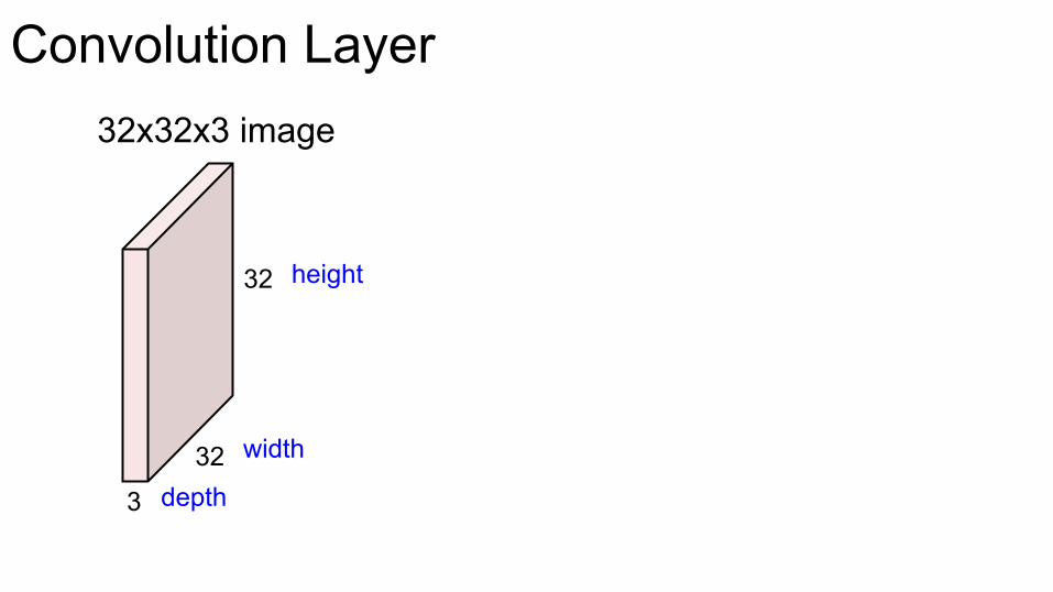
Convolution Layer 32x32x3 image
width
height
depth

32
32
3
Convolution Layer
5x5x3 filter
32x32x3 image
Convolve the filter with the image i.e. “slide over the image spatially, computing dot products”
32
32
3
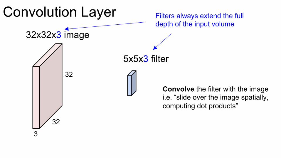
Convolution Layer
5x5x3 filter
32x32x3 image
Convolve the filter with the image i.e. “slide over the image spatially, computing dot products”
Filters always extend the full depth of the input volume

32
32
3
Convolution Layer 32x32x3 image 5x5x3 filter
1 number: the result of taking a dot product between the filter and a small 5x5x3 chunk of the image (i.e. 5*5*3 = 75-dimensional dot product + bias)

32
32
3
Convolution Layer 32x32x3 image 5x5x3 filter
convolve (slide) over all spatial locations
activation map
1
28
28
32
32
3
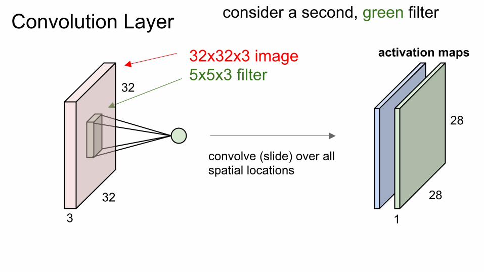
Convolution Layer 32x32x3 image 5x5x3 filter
convolve (slide) over all spatial locations
activation maps
1
28
28
consider a second, green filter
32
32
3
Convolution Layer
activation maps
6
28
28
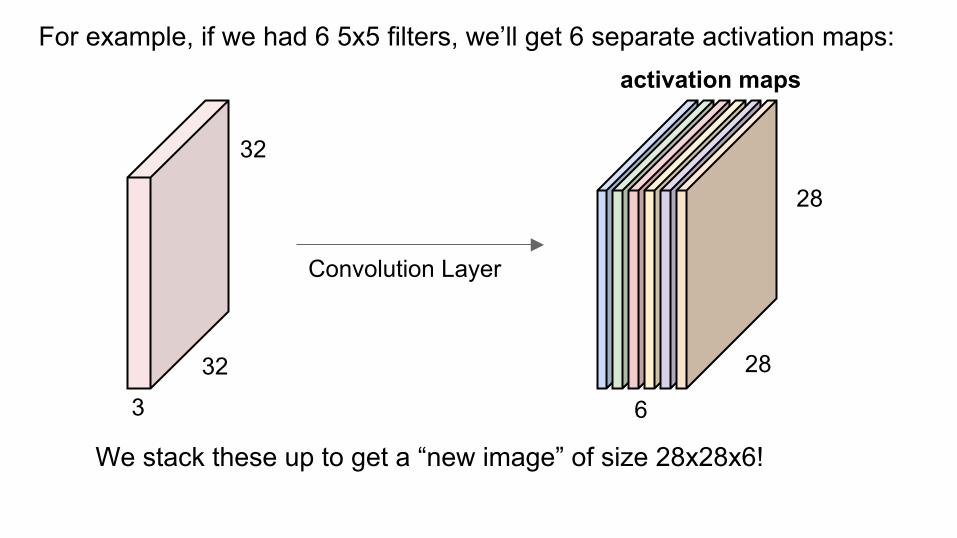
For example, if we had 6 5x5 filters, we’ll get 6 separate activation maps:
We stack these up to get a “new image” of size 28x28x6!

32
32
3
Convolution Layer
activation maps
6
28
28
For example, if we had 6 5x5 filters, we’ll get 6 separate activation maps:
We processed [32x32x3] volume into [28x28x6] volume. Q: how many parameters would this be if we used a fully connected layer instead?
32
32
3
Convolution Layer
activation maps
6
28
28
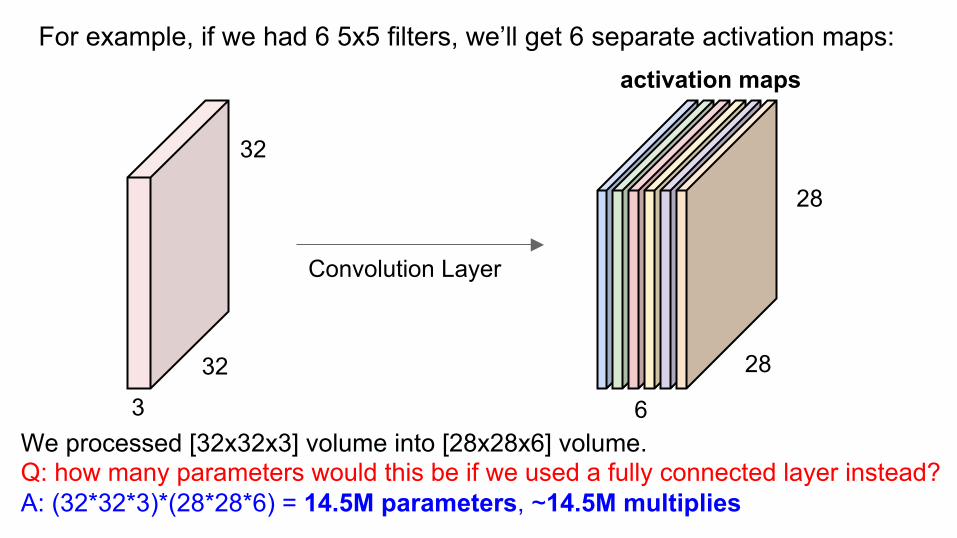
For example, if we had 6 5x5 filters, we’ll get 6 separate activation maps:
We processed [32x32x3] volume into [28x28x6] volume. Q: how many parameters would this be if we used a fully connected layer instead? A: (32*32*3)*(28*28*6) = 14.5M parameters, ~14.5M multiplies
32
32
3
Convolution Layer
activation maps
6
28
28
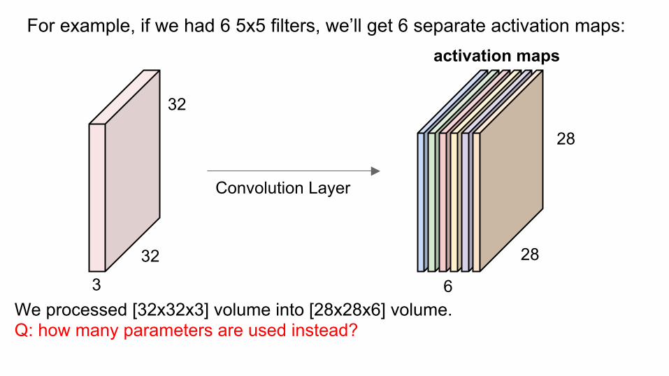
For example, if we had 6 5x5 filters, we’ll get 6 separate activation maps:
We processed [32x32x3] volume into [28x28x6] volume. Q: how many parameters are used instead?

32
32
3
Convolution Layer
activation maps
6
28
28
For example, if we had 6 5x5 filters, we’ll get 6 separate activation maps:
We processed [32x32x3] volume into [28x28x6] volume. Q: how many parameters are used instead? --- And how many multiplies? A: (5*5*3)*6 = 450 parameters
32
32
3
Convolution Layer
activation maps
6
28
28
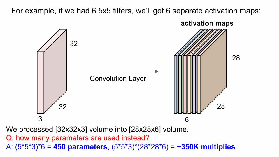
For example, if we had 6 5x5 filters, we’ll get 6 separate activation maps:
We processed [32x32x3] volume into [28x28x6] volume. Q: how many parameters are used instead? A: (5*5*3)*6 = 450 parameters, (5*5*3)*(28*28*6) = ~350K multiplies

example 5x5 filters (32 total)
We call the layer convolutional because it is related to convolution of two signals:
elementwise multiplication and sum of a filter and the signal (image)
one filter => one activation map

Preview: ConvNet is a sequence of Convolution Layers, interspersed with activation functions
32
32
3
28
28
6
CONV, ReLU e.g. 6 5x5x3 filters

Rectified Linear Units (ReLUs)
0.77 -0.11 0.11 0.33 0.55 -0.11 0.33
-0.11 1.00 -0.11 0.33 -0.11 0.11 -0.11
0.11 -0.11 1.00 -0.33 0.11 -0.11 0.55
0.33 0.33 -0.33 0.55 -0.33 0.33 0.33
0.55 -0.11 0.11 -0.33 1.00 -0.11 0.11
-0.11 0.11 -0.11 0.33 -0.11 1.00 -0.11
0.33 -0.11 0.55 0.33 0.11 -0.11 0.77
0.77

0.77 0
Rectified Linear Units (ReLUs)
0.77 -0.11 0.11 0.33 0.55 -0.11 0.33
-0.11 1.00 -0.11 0.33 -0.11 0.11 -0.11
0.11 -0.11 1.00 -0.33 0.11 -0.11 0.55
0.33 0.33 -0.33 0.55 -0.33 0.33 0.33
0.55 -0.11 0.11 -0.33 1.00 -0.11 0.11
-0.11 0.11 -0.11 0.33 -0.11 1.00 -0.11
0.33 -0.11 0.55 0.33 0.11 -0.11 0.77
0.77 0 0.11 0.33 0.55 0 0.33
Rectified Linear Units (ReLUs)
0.77 -0.11 0.11 0.33 0.55 -0.11 0.33
-0.11 1.00 -0.11 0.33 -0.11 0.11 -0.11
0.11 -0.11 1.00 -0.33 0.11 -0.11 0.55
0.33 0.33 -0.33 0.55 -0.33 0.33 0.33
0.55 -0.11 0.11 -0.33 1.00 -0.11 0.11
-0.11 0.11 -0.11 0.33 -0.11 1.00 -0.11
0.33 -0.11 0.55 0.33 0.11 -0.11 0.77

0.77 0 0.11 0.33 0.55 0 0.33
0 1.00 0 0.33 0 0.11 0
0.11 0 1.00 0 0.11 0 0.55
0.33 0.33 0 0.55 0 0.33 0.33
0.55 0 0.11 0 1.00 0 0.11
0 0.11 0 0.33 0 1.00 0
0.33 0 0.55 0.33 0.11 0 0.77
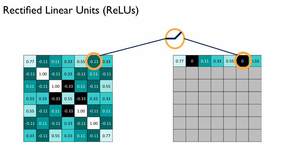
Rectified Linear Units (ReLUs)
0.77 -0.11 0.11 0.33 0.55 -0.11 0.33
-0.11 1.00 -0.11 0.33 -0.11 0.11 -0.11
0.11 -0.11 1.00 -0.33 0.11 -0.11 0.55
0.33 0.33 -0.33 0.55 -0.33 0.33 0.33
0.55 -0.11 0.11 -0.33 1.00 -0.11 0.11
-0.11 0.11 -0.11 0.33 -0.11 1.00 -0.11
0.33 -0.11 0.55 0.33 0.11 -0.11 0.77
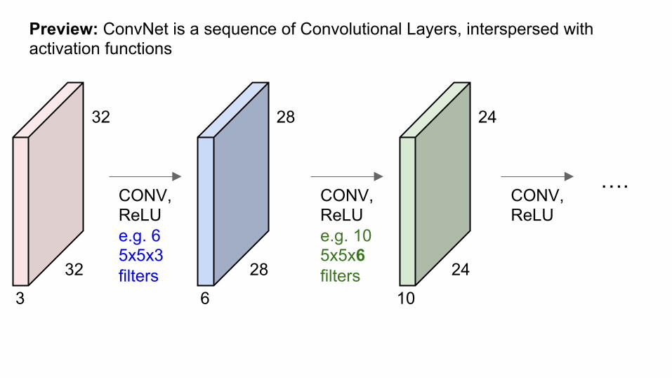
Preview: ConvNet is a sequence of Convolutional Layers, interspersed with activation functions
32
32
3
CONV, ReLU e.g. 6 5x5x3 filters 28
28
6
CONV, ReLU e.g. 10 5x5x6 filters
CONV, ReLU
….
10
24
24
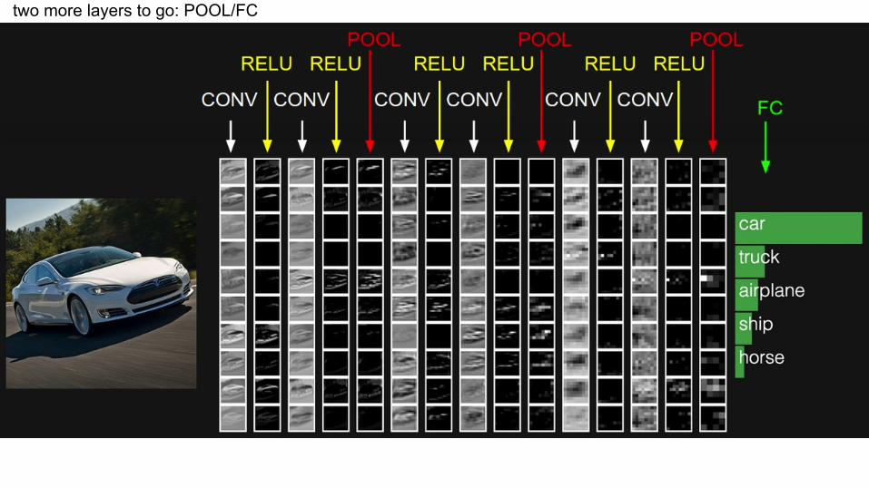
two more layers to go: POOL/FC
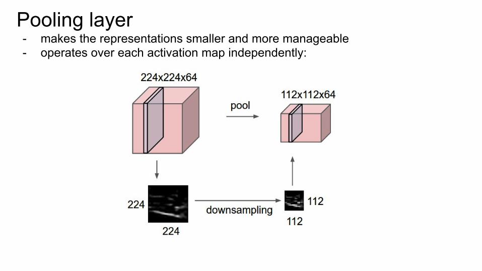
Pooling layer - makes the representations smaller and more manageable - operates over each activation map independently:

1 1 2 4
5 6 7 8
3 2 1 0
1 2 3 4
Single depth slice
x
y
max pool with 2x2 filters and stride 2 6 8
3 4
MAX POOLING

Fully Connected Layer (FC layer)
- Contains neurons that connect to the entire input volume, as in ordinary Neural Networks

Softmax
SCORES PROBABILITIES

http://cs.stanford.edu/people/karpathy/convnetjs/demo/cifar10.html
[ConvNetJS demo: training on CIFAR-10]
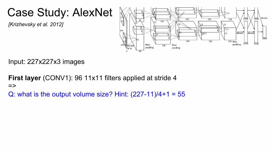
Case Study: AlexNet [Krizhevsky et al. 2012]
Input: 227x227x3 images First layer (CONV1): 96 11x11 filters applied at stride 4 => Q: what is the output volume size? Hint: (227-11)/4+1 = 55

Case Study: AlexNet [Krizhevsky et al. 2012]
Input: 227x227x3 images First layer (CONV1): 96 11x11 filters applied at stride 4 => Output volume [55x55x96] Q: What is the total number of parameters in this layer?

Case Study: AlexNet [Krizhevsky et al. 2012]
Input: 227x227x3 images First layer (CONV1): 96 11x11 filters applied at stride 4 => Output volume [55x55x96] Parameters: (11*11*3)*96 = 35K
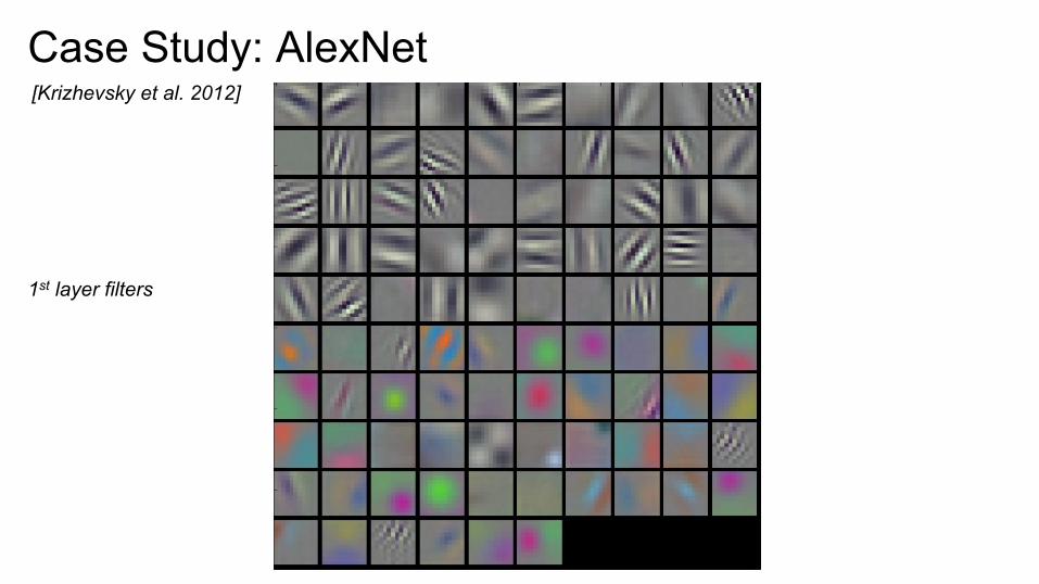
Case Study: AlexNet [Krizhevsky et al. 2012]
1st layer filters
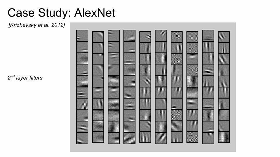
Case Study: AlexNet [Krizhevsky et al. 2012]
2nd layer filters
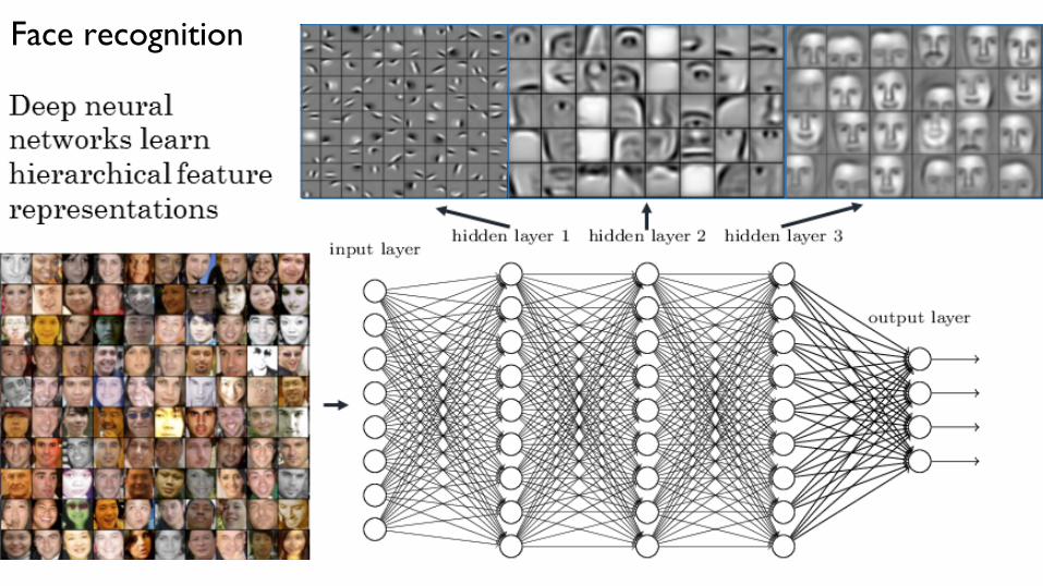
Face recognition

Case Study: AlexNet [Krizhevsky et al. 2012]
Full (simplified) AlexNet architecture: [227x227x3] INPUT [55x55x96] CONV1: 96 11x11 filters at stride 4, pad 0 [27x27x96] MAX POOL1: 3x3 filters at stride 2 [27x27x96] NORM1: Normalization layer [27x27x256] CONV2: 256 5x5 filters at stride 1, pad 2 [13x13x256] MAX POOL2: 3x3 filters at stride 2 [13x13x256] NORM2: Normalization layer [13x13x384] CONV3: 384 3x3 filters at stride 1, pad 1 [13x13x384] CONV4: 384 3x3 filters at stride 1, pad 1 [13x13x256] CONV5: 256 3x3 filters at stride 1, pad 1 [6x6x256] MAX POOL3: 3x3 filters at stride 2 [4096] FC6: 4096 neurons [4096] FC7: 4096 neurons [1000] FC8: 1000 neurons (class scores)
Compared to LeCun 1998: 1 DATA: - More data: 10^6 vs. 10^3 2 COMPUTE: - GPU (~100x speedup) 3 ALGORITHM: - Deeper: More layers (8 weight layers) - Fancy regularization (dropout) - Fancy non-linearity (ReLU)

Case Study: AlexNet [Krizhevsky et al. 2012]
Full (simplified) AlexNet architecture: [227x227x3] INPUT [55x55x96] CONV1: 96 11x11 filters at stride 4, pad 0 [27x27x96] MAX POOL1: 3x3 filters at stride 2 [27x27x96] NORM1: Normalization layer [27x27x256] CONV2: 256 5x5 filters at stride 1, pad 2 [13x13x256] MAX POOL2: 3x3 filters at stride 2 [13x13x256] NORM2: Normalization layer [13x13x384] CONV3: 384 3x3 filters at stride 1, pad 1 [13x13x384] CONV4: 384 3x3 filters at stride 1, pad 1 [13x13x256] CONV5: 256 3x3 filters at stride 1, pad 1 [6x6x256] MAX POOL3: 3x3 filters at stride 2 [4096] FC6: 4096 neurons [4096] FC7: 4096 neurons [1000] FC8: 1000 neurons (class scores)
Details/Retrospectives: - first use of ReLU - used Norm layers (not common anymore) - heavy data augmentation - dropout 0.5 - batch size 128 - SGD Momentum 0.9 - Learning rate 1e-2, reduced by 10 manually when val accuracy plateaus - L2 weight decay 5e-4 - 7 CNN ensemble: 18.2% -> 15.4%

Case Study: VGGNet [Simonyan and Zisserman, 2014]
best model
Only 3x3 CONV stride 1, pad 1 and 2x2 MAX POOL stride 2
11.2% top 5 error in ILSVRC 2013 -> 7.3% top 5 error

Case Study: GoogLeNet [Szegedy et al., 2014]
Inception module
ILSVRC 2014 winner (6.7% top 5 error)
Slide from Kaiming He’s recent presentation https://www.youtube.com/watch?v=1PGLj-uKT1w
Case Study: ResNet [He et al., 2015]
ILSVRC 2015 winner (3.6% top 5 error)

Case Study: ResNet [He et al., 2015]
224x224x3
spatial dimension only 56x56!

VGG: ~2-3 weeks training with 4 GPUs ResNet: ~2-3 weeks training with 4 GPUs
~$1K each

Addressing other tasks...

Transfer Learning
1. Train on Imagenet
3. Medium dataset: finetuning more data = retrain more of the network (or all of it)
2. Small dataset: feature extractor
Freeze these
Train this
Freeze these
Train this

Transfer Learning
CNN Features off-the-shelf: an Astounding Baseline for Recognition [Razavian et al, 2014]

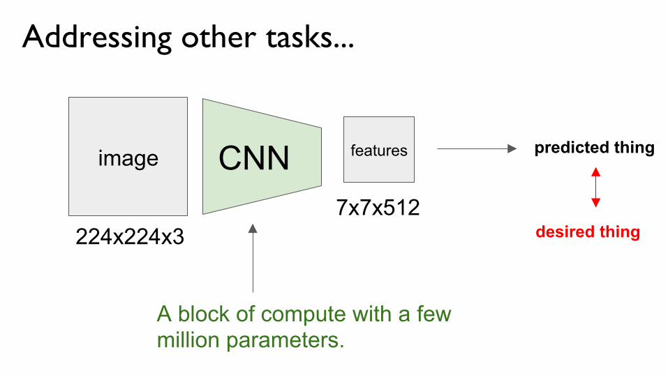
Addressing other tasks...
image CNN features
224x224x3
A block of compute with a few million parameters.
7x7x512
Addressing other tasks...
image CNN features
224x224x3
A block of compute with a few million parameters.
7x7x512
predicted thing
desired thing
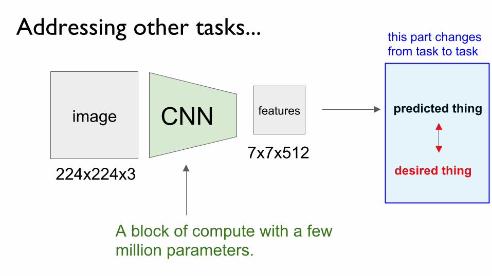
Addressing other tasks...
image CNN features
224x224x3
A block of compute with a few million parameters.
7x7x512
predicted thing
desired thing
this part changes from task to task
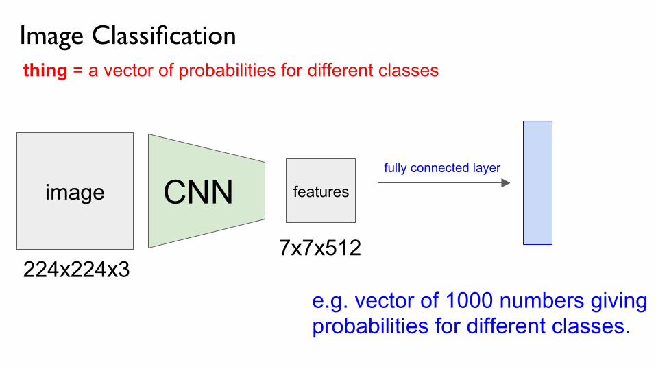
Image Classificationthing = a vector of probabilities for different classes
image CNN features
224x224x3 7x7x512
e.g. vector of 1000 numbers giving probabilities for different classes.
fully connected layer
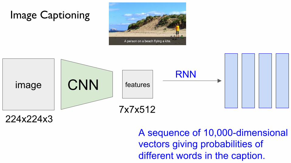
Image Captioning
image CNN features
224x224x3 7x7x512
A sequence of 10,000-dimensional vectors giving probabilities of different words in the caption.
RNN
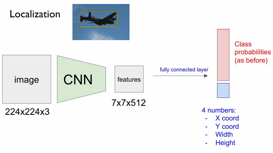
Localization
image CNN features
224x224x3 7x7x512
fully connected layer
Class probabilities (as before)
4 numbers: - X coord - Y coord - Width - Height

Reinforcement Learning
image CNN features
160x210x3
fully connected
e.g. vector of 8 numbers giving probability of wanting to take any of the 8 possible ATARI actions.
Mnih et al. 2015

ConvNets are everywhere…
e.g. Google Photos search
Face Verification, Taigman et al. 2014 (FAIR)
Self-driving cars [Goodfellow et al. 2014]
Ciresan et al. 2013
Turaga et al 2010
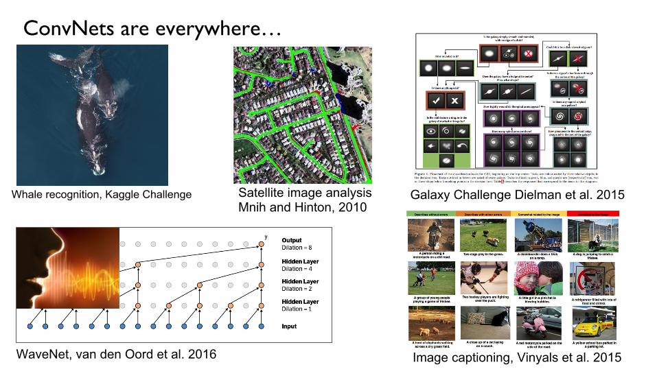
ConvNets are everywhere…
Whale recognition, Kaggle Challenge Satellite image analysis Mnih and Hinton, 2010
Galaxy Challenge Dielman et al. 2015
WaveNet, van den Oord et al. 2016 Image captioning, Vinyals et al. 2015

ConvNets are everywhere…
AlphaGo, Silver et al 2016
VizDoom
StarCraft

ConvNets are everywhere…
DeepDream reddit.com/r/deepdream
NeuralStyle, Gatys et al. 2015 deepart.io, Prisma, etc.
Practical considerations when applying ConvNets

What hardware do I use? Buy your own machine: - NVIDIA DIGITS DevBox (TITAN X GPUs) - NVIDIA DGX-1 (P100 GPUs)
Build your own machine: https://graphific.github.io/posts/building-a-deep-learning-dream-machine/
GPUs in the cloud: - Amazon AWS (GRID K520 :( ) - Microsoft Azure (soon); 4x K80 GPUs - Cirrascale (“rent-a-box”)

What framework do I use?
Caffe
Torch
Theano
Lasagne Keras
TensorFlow
Mxnet chainer Nervana’s Neon Microsoft’s CNTK Deeplearning4j ...
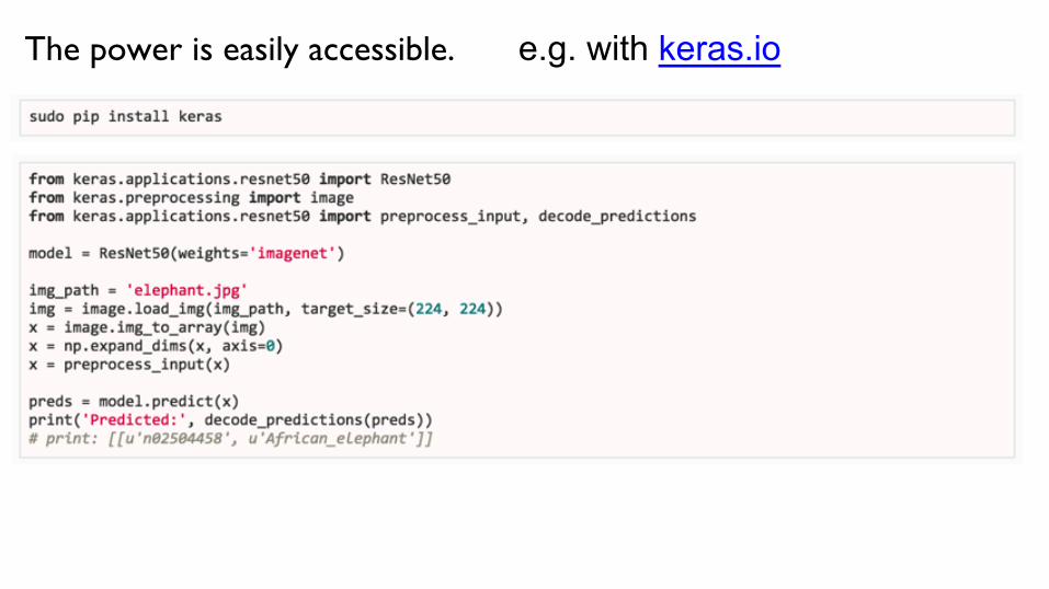
e.g. with keras.io The power is easily accessible.

Q: How do I know what architecture/hyperparameters to use?
A: don’t be a hero. 1. Take whatever works best on ILSVRC (latest ResNet) 2. Download a pretrained model 3. Potentially add/delete some parts of it 4. Finetune it on your application. 5. Play with the regularization strength (dropout rates)
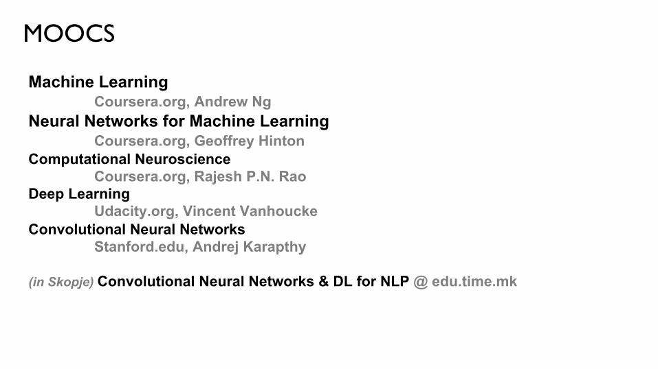
MOOCS
Machine Learning Coursera.org, Andrew Ng
Neural Networks for Machine Learning Coursera.org, Geoffrey Hinton
Computational Neuroscience Coursera.org, Rajesh P.N. Rao
Deep Learning Udacity.org, Vincent Vanhoucke
Convolutional Neural Networks Stanford.edu, Andrej Karapthy
(in Skopje) Convolutional Neural Networks & DL for NLP @ edu.time.mk