Deep Neural Networks Reveal a Gradient in the

Complexity of Neural Representations across the

Brain’s Ventral Visual Pathway

Umut Guclu∗1 and Marcel A. J. van Gerven1

1Radboud University Nijmegen, Donders Institute for Brain,Cognition and Behaviour, Nijmegen, the Netherlands

November 25, 2014

Abstract

Converging evidence suggests that the mammalian ventral visual path-way encodes increasingly complex stimulus features in downstream ar-eas. Using deep convolutional neural networks, we can now quantitativelydemonstrate that there is indeed an explicit gradient for feature complex-ity in the ventral pathway of the human brain. Our approach also allowsstimulus features of increasing complexity to be mapped across the humanbrain, providing an automated approach to probing how representationsare mapped across the cortical sheet. Finally, it is shown that deep convo-lutional neural networks allow decoding of representations in the humanbrain at a previously unattainable degree of accuracy, providing a moresensitive window into the human brain.

1 Introduction

Human beings are extremely adept at recognizing complex objects based onelementary visual sensations. Object recognition appears to be solved in themammalian brain via a cascade of neural computations along the visual ventralstream that represents increasingly complex stimulus features, which derive fromthe retinal input [1]. That is, neurons in early visual areas have small recep-tive fields and respond to simple features such as edge orientation [2], whereasneurons further along the ventral pathway have larger receptive fields, are moreinvariant to transformations and can be selective for complex shapes [3].

Despite converging evidence concerning the steady progression in featurecomplexity along the ventral stream, this progression has never been properlyquantified across multiple regions in the human ventral stream. Furthermore,while the receptive fields in early visual area V1 have been properly characterizedin terms of preferred orientation, location and spatial frequency [4], exactly whatstimulus features are represented in downstream areas is more heavily debated[5].

∗Correspondence to: u.guclu@donders.ru.nl

1

arX

iv:1

411.

6422

v1 [

q-bi

o.N

C]

24

Nov

201

4

In order to isolate how stimulus features at different representational com-plexities are represented across the cortical sheet, we made use of a deep con-volutional neural network (CNN). Deep CNNs consist of multiple layers wheredeeper layers can be shown to respond to increasingly complex stimulus featuresand provide state-of-the-art object recognition performance in computer vision[6]. We used the representations that emerge after training a deep CNN in or-der to predict blood-oxygen-level dependent (BOLD) hemodynamic responsesto complex naturalistic stimuli in progressively downstream areas of the ventralstream, moving from striate area V1 along extrastriate areas V2 and V4, all theway up to area LOC in posterior inferior temporal (IT) cortex.

We used individual layers of the neural network to predict single voxel re-sponses to natural images. This allowed us to isolate different voxel groups,whose responses are best predicted by a particular layer in the neural network.Using this approach, we can determine how layer depth correlates with the posi-tion of voxels in the visual hierarchy. Furthermore, by testing to what extent in-dividual features in the neural network can predict voxel responses, we can maphow individual low-, mid- and high-level stimulus features are represented acrossthe ventral stream. This provides a unique and fully automated approach to de-termine how stimulus features of increasing complexity are represented acrossthe visual stream. Finally, we show that the predictions of neural responsesafforded by our framework give rise to state-of-the-art decoding performance,allowing identification of perceived stimuli from observed BOLD responses.

2 Framework

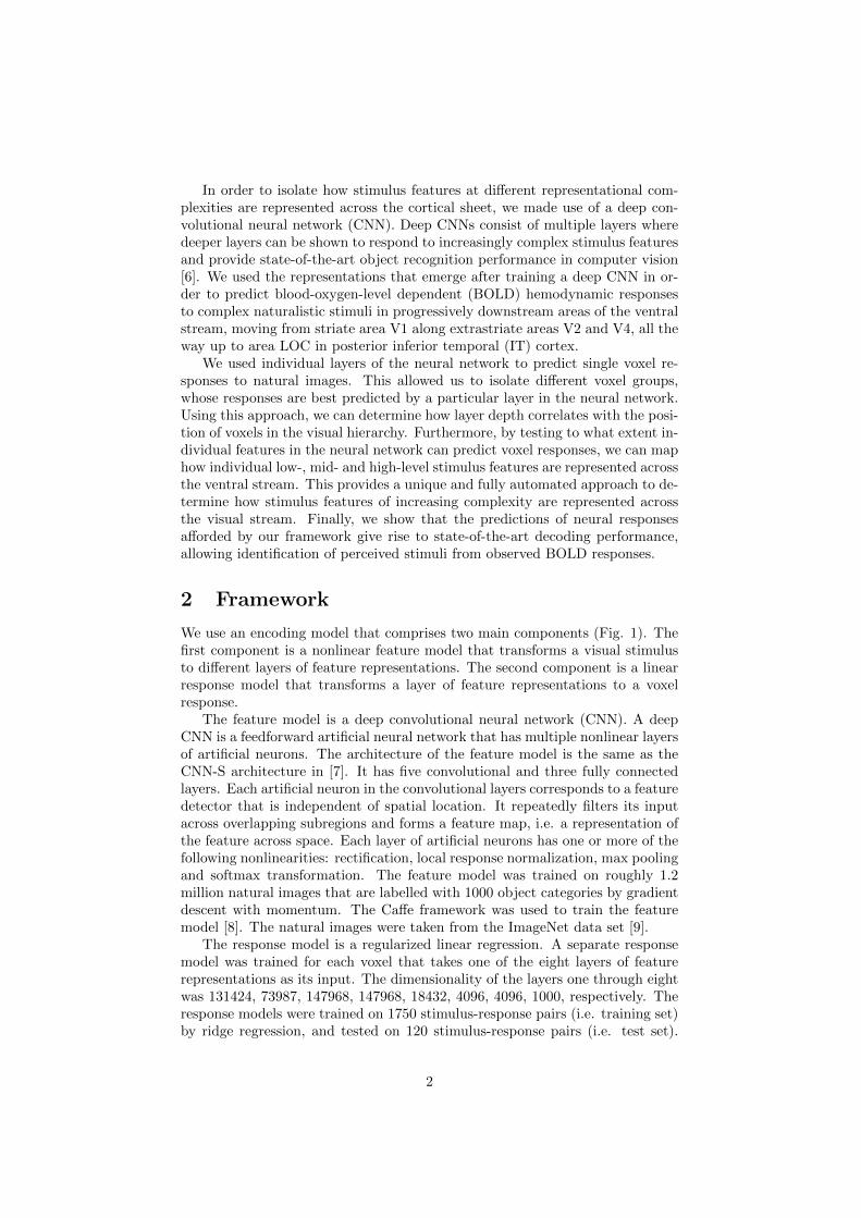
We use an encoding model that comprises two main components (Fig. 1). Thefirst component is a nonlinear feature model that transforms a visual stimulusto different layers of feature representations. The second component is a linearresponse model that transforms a layer of feature representations to a voxelresponse.

The feature model is a deep convolutional neural network (CNN). A deepCNN is a feedforward artificial neural network that has multiple nonlinear layersof artificial neurons. The architecture of the feature model is the same as theCNN-S architecture in [7]. It has five convolutional and three fully connectedlayers. Each artificial neuron in the convolutional layers corresponds to a featuredetector that is independent of spatial location. It repeatedly filters its inputacross overlapping subregions and forms a feature map, i.e. a representation ofthe feature across space. Each layer of artificial neurons has one or more of thefollowing nonlinearities: rectification, local response normalization, max poolingand softmax transformation. The feature model was trained on roughly 1.2million natural images that are labelled with 1000 object categories by gradientdescent with momentum. The Caffe framework was used to train the featuremodel [8]. The natural images were taken from the ImageNet data set [9].

The response model is a regularized linear regression. A separate responsemodel was trained for each voxel that takes one of the eight layers of featurerepresentations as its input. The dimensionality of the layers one through eightwas 131424, 73987, 147968, 147968, 18432, 4096, 4096, 1000, respectively. Theresponse models were trained on 1750 stimulus-response pairs (i.e. training set)by ridge regression, and tested on 120 stimulus-response pairs (i.e. test set).

2

1, 2, 3, 4

96 1000512512512256 4096 40963

6

224

37 17 17 17

1 1 1

37 17 17 17 6 1 1 1224

3 7

7

96 5

5

256 3

3

512 3

3

512 3

3

A

B

Stimulus Feature Response

CNN linear map

1 conv, 2 ReLU, 3 LRN, 4 maxpool, 5 FC, 6 soft-max

1, 2, 4 1, 2 1, 2 1, 2, 4 5, 2 5, 2 5, 6

Figure 1: Framework. (A) Schematic of the encoding model. The encodingmodel transforms a visual stimulus to a voxel response in two stages. First,the deep convolutional neural network (CNN) transforms the visual stimulus toa layer of feature representations. Then, a linear map transforms the layer offeature representations to a voxel response. (B) Schematic of the deep CNN.The deep CNN transforms a visual stimulus to different layers of feature repre-sentations. It has five convolutional and three fully connected layers of artificialneurons. Each artificial neuron in the convolutional layers repeatedly filters itsinput across overlapping subregions and forms a feature map. Each layer ofartificial neurons has one or more of the following nonlinearities: rectification,local response normalization, max pooling and softmax transformation.

The stimulus-response pairs were taken from the vim-1 data set [10] that wasoriginally published in [11, 12]. The stimulus-response pairs consist of grayscalenatural images spanning 20 × 20 degrees of visual angle and stimulus-evokedpeak BOLD hemodynamic responses of 25915 voxels in the occipital cortex ofone subject (i.e. Subject 1). The details of the experimental procedures arepresented in [11]. Unless otherwise stated, all significance levels are p ≤ 0.01and Bonferroni corrected for multiple comparisons when required.

3 Results

We used five-fold cross-validation to assign each of the 25915 voxels to one of theeight layers of the deep CNN (Fig. 2A). That is, each voxel was assigned to thelayer of the deep CNN that resulted in the lowest cross-validation error on thetraining set. Those voxels whose prediction accuracy was not significantly betterthan chance were discarded. The reason for nonsignificant prediction accuracyof these voxels could be either their low signal-to-noise ratio (SNR) or that noneof the layers of the deep CNN reproduced their behavior. As a result, 13% ofthe voxels in the occipital cortex were further analyzed. The response models ofthese voxels were trained on the entire training set and evaluated on the test set.The prediction accuracy of a voxel was defined as the Pearson product-momentcorrelation coefficient (r) between its observed and predicted responses on thetest set. For a group of voxels, the median correlation coefficient was used toexpress its prediction accuracy.

We grouped the voxels that were assigned to the same layer. While theprediction accuracy of each of the voxel groups was significantly above zero, itdecreased from low- to high-layer voxel groups (Fig. 2B). The prediction accu-

3

A B

V1 V2 V3 V3A V3B V4 LOCVisual area

1 2 3 4 5 6 7 8Layer assignment

0 0.25 0.5 0.75 1Prediction accuracy (r)

s↑

a ← p → a↓

i

LH LHRH RH

V1 V2 V3 V3A V3B V4 LOCVisual area

s↑

a ← p → a↓

i

Figure 2: Encoding results of the significant voxels across the cortical surface.LH, RH, p, a, s and i denote left hemisphere, right hemisphere, posterior, an-terior, superior and inferior, respectively. (A) Layer assignment of the voxelsacross the cortical surface. Each voxel is assigned to the layer of the deep CNNthat resulted in the lowest cross-validation error on the training set. (B) Predic-tion accuracy of the voxels across the cortical surface. The prediction accuracyof a voxel is defined as the Pearson product-moment correlation coefficient (r)between its observed and predicted responses on the test set.

racy of the voxel groups one through eight was 0.42, 0.50, 0.39, 0.29, 0.27, 0.24,0.27 and 0.16, respectively (SE ≤ 0.02). The prediction accuracy was signifi-cantly correlated with the mean activity of the layers across the training set andthe SNR of the voxels. This suggests that the difference in the prediction accu-racy of the low- and high-layer voxel groups can be explained by the differencesin the mean activity of the layers and the SNR of the voxels.

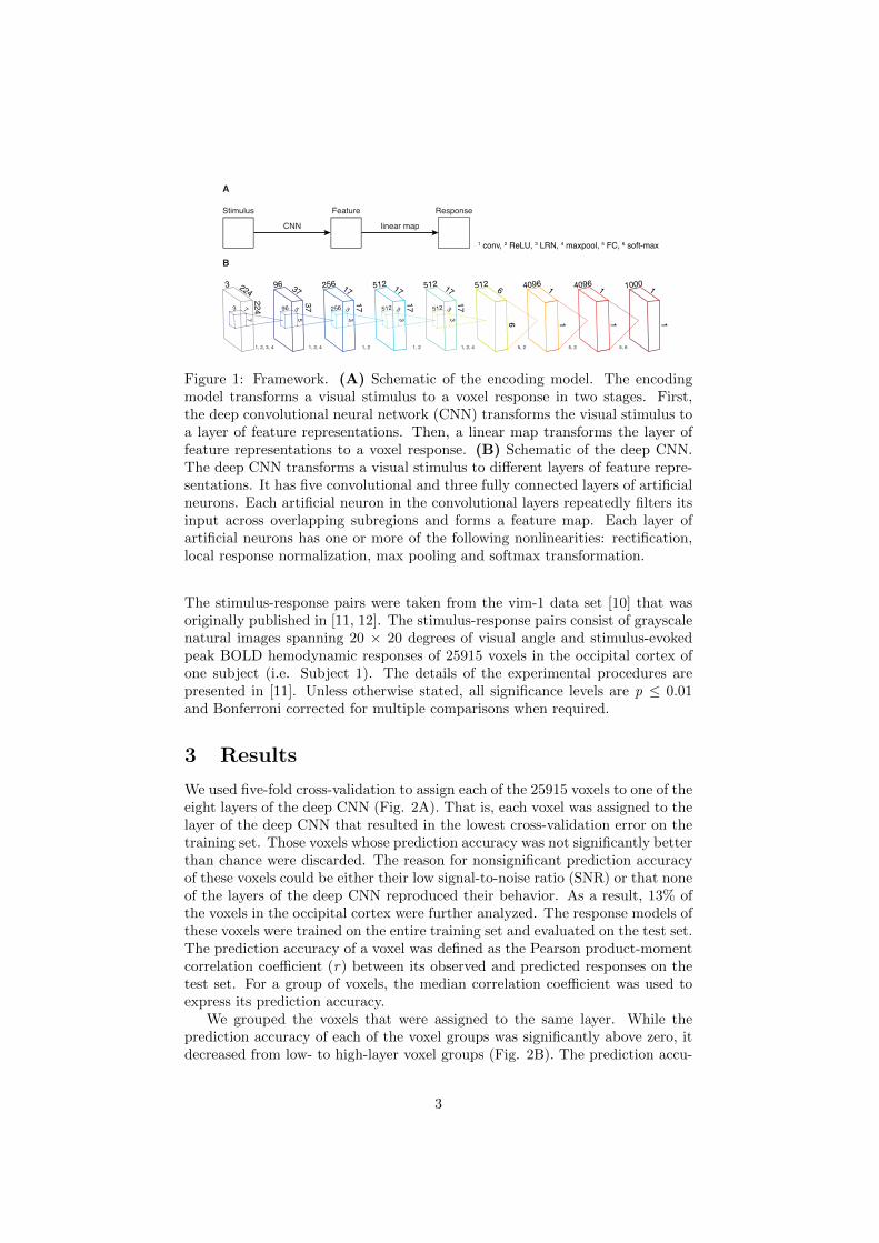
Different voxel groups were systematically clustered around different pointson the cortical surface such that an increase in the layer of the voxel groups wasobserved when moving from posterior to anterior points on the cortical surface.The responses of the successive voxel groups were more partially correlatedthan those of the non-successive voxels groups (Fig. 3A). The receptive fieldsof the voxels in each voxel group covered almost the entire field of view, withmore voxels dedicated to foveal than peripheral vision (Fig. 3B). While therewas a degree of overlap between the internal representations of the successivevoxel groups, those of the low-layers resembled Gabor wavelets and textures, andthose of the high-layers resembled object parts and objects (Fig. 3C). The meanKolmogorov complexity (K ) of the internal representations was significantlycorrelated with their layer assignment (Fig. 3D). Taken together, these resultssuggest that i) each voxel group contains almost a full representation of visualspace, ii) visual information travels mostly between neighboring voxel groups,and iii) moving along the voxel groups, their receptive fields increase in size,latency and complexity.

Given that these properties resemble those of the visual areas on the mainafferent pathway of the ventral stream [14], it is interesting to consider howthese voxel groups are distributed across V1, V2, V4 and LOC. We found asystematic overlap between these voxel groups and visual areas (Fig. 4A). Themean layer assignment of the V1, V2, V4 and LOC voxels was 1.8, 2.3, 3.0and 4.9, respectively (SE ≤ 0.1). That is, most of the low-layer voxels were

4

Fully connected

Layer 6 Layer 7 Layer 8Layer 1 Layer 2 Layer 3 Layer 4 Layer 5

D

A

B

C

Figure 3: Properties of the voxel groups. (A) Partial correlations between thepredicted responses of each pair of voxel groups, controlling for the predictedresponses of the remaining voxel groups. The width of the lines are proportionalto the partial correlations. (B) Distribution of the receptive field locations.(C) Examples of the internal representations. The internal representations arevisualized using a deconvolutional network [13]. (D) Mean field of view (FOV)and Kolmogorov complexity (K ) of the internal representations. FOV is takento be the size of the filters. K is taken to be the compressed file size of theinternal representations.

located in early visual areas, whereas most of the high-layer voxels were locatedin downstream visual areas. Most of the fully connected voxels were located invisual areas anterior to LOC. The prediction accuracy of the V1, V2, V4 andLOC voxels was 0.51, 0.46, 0.30 and 0.30, respectively (SE ≤ 0.02) (Fig. 4B).That of the remaining voxels were 0.28 (SE ≤ 0.01). However, in contrast tothe 30% of the V1, V2, V4 and LOC voxels that were significant, only 8% ofthe remaining voxels were significant. These results suggest that this deep CNNreproduces the behavior of the visual areas on the main afferent pathway of theventral stream.

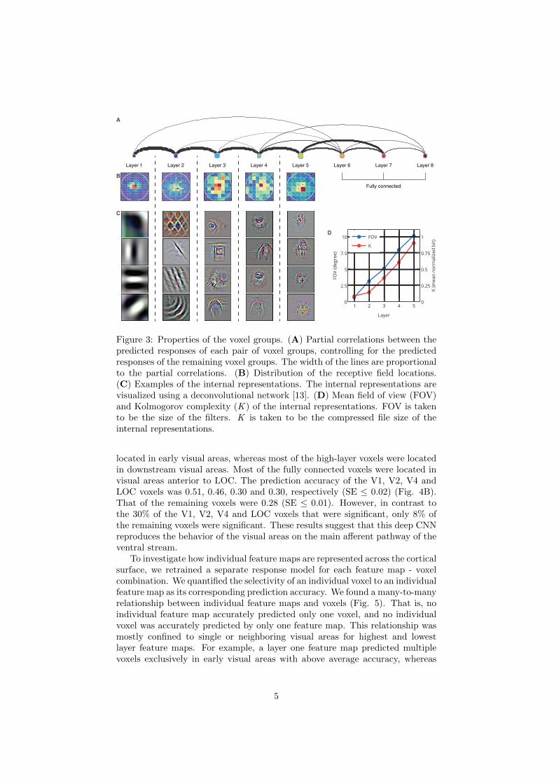
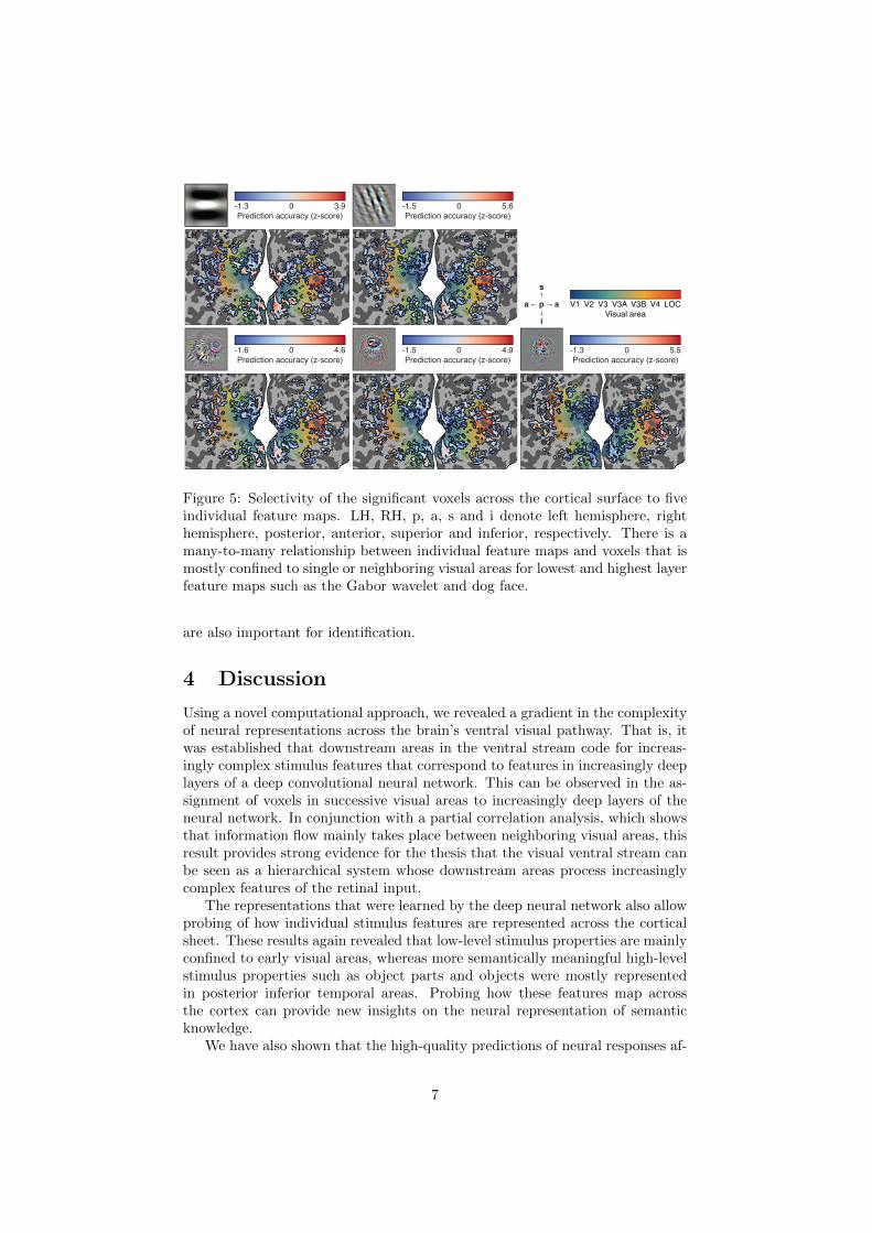
To investigate how individual feature maps are represented across the corticalsurface, we retrained a separate response model for each feature map - voxelcombination. We quantified the selectivity of an individual voxel to an individualfeature map as its corresponding prediction accuracy. We found a many-to-manyrelationship between individual feature maps and voxels (Fig. 5). That is, noindividual feature map accurately predicted only one voxel, and no individualvoxel was accurately predicted by only one feature map. This relationship wasmostly confined to single or neighboring visual areas for highest and lowestlayer feature maps. For example, a layer one feature map predicted multiplevoxels exclusively in early visual areas with above average accuracy, whereas

5

A B

1 2 3 4 5 6 7 8Layer assignment

0 0.25 0.5 0.75 1Prediction accuracy (r)

LOCV4V2V1 LOCV4V2V1

Figure 4: Encoding results of the significant voxels across V1, V2, V4 and LOC.(A) Layer assignment of the voxels across V1, V2, V4 and LOC. Each voxel isassigned to the layer of the deep CNN that resulted in the lowest cross-validationerror on the training set. (B) Prediction accuracy of the voxels across V1, V2,V4 and LOC. The prediction accuracy of a voxel is defined as the Pearsonproduct-moment correlation coefficient (r) between its observed and predictedresponses on the test set.

a layer five feature map predicted multiple voxels exclusively in downstreamvisual areas with above average accuracy.

Given the highly significant accuracy with which individual voxel responsescan be predicted, it is natural to ask to what extent the deep model allowsdecoding of a perceived stimulus from observed multiple voxel responses alone.To answer this question, we evaluated three decoding models: a low-level (V1 +V2), a high-level (V4 + LOC) and a combined (V1 + V2 + V4 + LOC) decodingmodel. Given observed multiple voxel responses, the low-level decoding modelcorrectly identified a stimulus from a set of 120 potential stimuli at 98% accu-racy, whereas the high-level decoding model correctly identified a stimulus fromthe same set of potential stimuli at 55% accuracy. As the number of potentialstimuli was increased from 120 to 1870, the identification performance of thelow- and high-level decoding models decreased to an accuracy of 95% and 38%,respectively. The difference between the identification performance of the low-and high-level decoding models is not surprising since it would be more likely fortwo different stimuli to have ambiguously similar high-level representations thanlow-level representations. In fact, when we analyzed the misidentified stimuli,we found that the high-level model could most of the times identify a potentialstimulus that is semantically but not structurally close to the target stimulus.

This result suggests that the combination of the low- and high-level decodingmodels would have a higher identification accuracy since the higher level voxelscan be used to resolve the ambiguities in the feature representations of the lowerlevel voxels and vice versa. As expected, the combined decoding model had ahigher identification accuracy than either of the low- and high-level decodingmodels alone. It identified the correct stimulus from a set of 120 potentialstimuli at 100% accuracy. As the number of potential stimuli was increasedalmost 16-fold, there was no decrease in the identification accuracy. This resultis a significant improvement on the earlier results in the literature where low-level features were used [11, 15], suggesting that mid- and high-level features

6

V1 V2 V3 V3A V3B V4 LOCVisual area

s↑

a ← p → a↓

i

-1.3 0 3.9Prediction accuracy (z-score)

-1.5 0 5.6Prediction accuracy (z-score)

-1.6 0 4.6Prediction accuracy (z-score)

-1.5 0 4.9Prediction accuracy (z-score)

-1.3 0 5.5Prediction accuracy (z-score)

LH RH LH RH

LH RH LH RH LH RH

Figure 5: Selectivity of the significant voxels across the cortical surface to fiveindividual feature maps. LH, RH, p, a, s and i denote left hemisphere, righthemisphere, posterior, anterior, superior and inferior, respectively. There is amany-to-many relationship between individual feature maps and voxels that ismostly confined to single or neighboring visual areas for lowest and highest layerfeature maps such as the Gabor wavelet and dog face.

are also important for identification.

4 Discussion

Using a novel computational approach, we revealed a gradient in the complexityof neural representations across the brain’s ventral visual pathway. That is, itwas established that downstream areas in the ventral stream code for increas-ingly complex stimulus features that correspond to features in increasingly deeplayers of a deep convolutional neural network. This can be observed in the as-signment of voxels in successive visual areas to increasingly deep layers of theneural network. In conjunction with a partial correlation analysis, which showsthat information flow mainly takes place between neighboring visual areas, thisresult provides strong evidence for the thesis that the visual ventral stream canbe seen as a hierarchical system whose downstream areas process increasinglycomplex features of the retinal input.

The representations that were learned by the deep neural network also allowprobing of how individual stimulus features are represented across the corticalsheet. These results again revealed that low-level stimulus properties are mainlyconfined to early visual areas, whereas more semantically meaningful high-levelstimulus properties such as object parts and objects were mostly representedin posterior inferior temporal areas. Probing how these features map acrossthe cortex can provide new insights on the neural representation of semanticknowledge.

We have also shown that the high-quality predictions of neural responses af-

7

forded by deep neural networks allow accurate decoding of complex stimuli fromobserved responses. The resulting decoding performance significantly improveson the performance which can be obtained with other established approachesthat do not incorporate mid- to high-level stimulus features [11, 15].

Our use of deep neural networks to probe cortical representations is in linewith the emerging use of sophisticated techniques that are rooted in statisticalmachine learning. For instance, in previous work, we have shown that deep beliefnetworks, which can learn stimulus features in a fully unsupervised manner,allow decoding of stimuli from observed neural responses [16]. Recently, itwas shown that performance-optimized hierarchical models can predict single-neuron responses in area IT of the macaque monkey [17]. Our current worksignificantly expands on these important results in (i) showing that there isan explicit gradient for object complexity in the ventral pathway of the humanbrain, (ii) providing an explicit visualization of features in deep layers of a neuralnetwork that are subsequently mapped across cortex and (iii) demonstratingthat deep neural networks allow decoding of representations in the human brainat a previously unattainable degree of accuracy, providing a sensitive windowinto the human brain.

References

[1] E. Kobatake and K. Tanaka, “Neuronal selectivities to complex object fea-tures in the ventral visual pathway of the macaque cerebral cortex,” Journalof Neurophysiology, vol. 71, no. 3, pp. 856–67, 1994.

[2] D. H. Hubel and T. N. Wiesel, “Receptive fields, binocular interaction andfunctional architecture in the cat’s visual cortex,” The Journal of Physiol-ogy, vol. 160, no. 3, pp. 106–54, 1962.

[3] C. P. Hung, G. Kreiman, T. Poggio, and J. J. DiCarlo, “Fast readout ofobject identity from macaque inferior temporal cortex,” Science, vol. 310,no. 5749, pp. 863–6, 2005.

[4] J. P. Jones and L. A. Palmer, “An evaluation of the two-dimensional Gaborfilter model of simple receptive fields in cat striate cortex,” Journal ofNeurophysiology, vol. 58, no. 6, pp. 1233–58, 1987.

[5] K. Grill-Spector, “What has fMRI taught us about object recognition?,”in Object Categorization: Computer and Human Vision Perspectives (S. J.Dickinson, A. Leonardis, B. Schiele, and M. J. Tarr, eds.), Cambridge Uni-versity Press, 2009.

[6] A. Krizhevsky, I. Sutskever, and G. E. Hinton, “ImageNet classificationwith deep convolutional neural networks,” in Advances in Neural Informa-tion Processing Systems, pp. 1097–1105, 2012.

[7] K. Chatfield, K. Simonyan, A. Vedaldi, and A. Zisserman, “Return of thedevil in the details: Delving deep into convolutional nets,” in British Ma-chine Vision Conference, 2014.

8

[8] Y. Jia, E. Shelhamer, J. Donahue, S. Karayev, J. Long, R. Girshick,S. Guadarrama, and T. Darrell, “Caffe: Convolutional architecture for fastfeature embedding,” arXiv preprint arXiv:1408.5093, 2014.

[9] J. Deng, W. Dong, R. Socher, L.-J. Li, K. Li, and L. Fei-Fei, “ImageNet: Alarge-scale hierarchical image database,” in IEEE Conference on ComputerVision and Pattern Recognition, pp. 248–255, 2009.

[10] K. N. Kay, T. Naselaris, and J. L. Gallant, “fMRI of human visual areasin response to natural images.” CRCNS.org, 2011.

[11] K. N. Kay, T. Naselaris, R. J. Prenger, and J. L. Gallant, “Identifyingnatural images from human brain activity,” Nature, vol. 452, no. 7185,pp. 352–5, 2008.

[12] T. Naselaris, R. J. Prenger, K. N. Kay, M. Oliver, and J. L. Gallant,“Bayesian reconstruction of natural images from human brain activity,”Neuron, vol. 63, no. 6, pp. 902–15, 2009.

[13] M. D. Zeiler and R. Fergus, “Visualizing and understanding convolutionalnetworks,” arXiv preprint arXiv:1311.2901, 2013.

[14] L. Zhaoping, Understanding Vision: Theory, Models, and Data. OxfordUniversity Press, 2014.

[15] U. Guclu and M. A. J. van Gerven, “Unsupervised feature learning improvesprediction of human brain activity in response to natural images,” PLoSComputational Biology, vol. 10, no. 8, p. e1003724, 2014.

[16] M. A. J. van Gerven, F. P. de Lange, and T. Heskes, “Neural decodingwith hierarchical generative models,” Neural Computation, vol. 22, no. 12,pp. 3127–42, 2010.

[17] D. L. Yamins, H. Hong, C. Cadieu, and J. J. DiCarlo, “Hierarchical modularoptimization of convolutional networks achieves representations similar tomacaque IT and human ventral stream,” in Advances in Neural InformationProcessing Systems, pp. 3093–3101, 2013.

9