deep reinforcement learning for adaptive network slicing
TRANSCRIPT

1
Deep Reinforcement Learning for AdaptiveNetwork Slicing in 5G for Intelligent Vehicular
Systems and Smart CitiesAlmuthanna Nassar, and Yasin Yilmaz, Senior Member, IEEE
Electrical Engineering Department, University of South Florida, Tampa, FL 33620, USAE-mails: {[email protected]; [email protected]}
Abstract—Intelligent vehicular systems and smart city appli-cations are the fastest growing Internet of things (IoT) imple-mentations at a compound annual growth rate of 30%. In viewof the recent advances in IoT devices and the emerging newbreed of IoT applications driven by artificial intelligence (AI),fog radio access network (F-RAN) has been recently introducedfor the fifth generation (5G) wireless communications to overcomethe latency limitations of cloud-RAN (C-RAN). We consider thenetwork slicing problem of allocating the limited resources atthe network edge (fog nodes) to vehicular and smart city userswith heterogeneous latency and computing demands in dynamicenvironments. We develop a network slicing model based on acluster of fog nodes (FNs) coordinated with an edge controller(EC) to efficiently utilize the limited resources at the networkedge. For each service request in a cluster, the EC decides whichFN to execute the task, i.e., locally serve the request at the edge,or to reject the task and refer it to the cloud. We formulatethe problem as infinite-horizon Markov decision process (MDP)and propose a deep reinforcement learning (DRL) solution toadaptively learn the optimal slicing policy. The performance ofthe proposed DRL-based slicing method is evaluated by com-paring it with other slicing approaches in dynamic environmentsand for different scenarios of design objectives. Comprehensivesimulation results corroborate that the proposed DRL-based ECquickly learns the optimal policy through interaction with theenvironment, which enables adaptive and automated networkslicing for efficient resource allocation in dynamic vehicular andsmart city environments.
Index Terms—Intelligent Vehicular Systems, Network Slicing,Deep Reinforcement Learning, Edge Computing, Fog RAN.
I. INTRODUCTION
The fifth generation (5G) wireless communication systemswill enable massive Internet of Things (IoT) with deepercoverage, very high data rates of multi giga-bit-per-second(Gbps), ultra-low latency, and extremely reliable mobile con-nectivity [1], [2]. It is anticipated that the IoT devices willconstitute the 50% of the 29.3 billion connected devicesglobally by 2023, where Internet of Vehicles (IoV) and smartcity applications are the fastest growing IoT implementationsat annual growth rates of 30% and 26%, respectively [3]. Theemerging new breed of IoT applications which involve videoanalytics, augmented reality (AR), virtual reality (VR), andartificial intelligence (AI) will produce an annual worldwidedata volume of 4.8 zettabyte by 2022, which is more than180 times the data traffic in 2005 [4]. Equipped with varietyof sensors, radars, lidars, ultra-high definition (UHD) videocameras, GPS, navigation system, and infotainment facilities,
a connected and autonomous vehicle (CAV) will generate 4.0terabyte of data in a single day, of which 1.0 gigabyte needto be processed every second [5].
A. Cloud and Fog RAN
Through centralization of network functionalities via virtu-alization, cloud radio access network (C-RAN) architectureis proposed to address the big data challenges of massiveIoT. In C-RAN, densely-deployed disseminated remote radiounits (RRUs) are connected through high capacity fronthaultrunks to a powerful cloud controller (CC) where they sharea vast pooling of storage and baseband units (BBUs) [6]. Thecentralized computing, processing, and collaborative radio inC-RAN improves network security, flexibility, availability, andspectral efficiency. It also simplifies network operations andmanagement, enhances capacity, and reduces energy usage[7]. However, considering the fast growing demands of IoTdeployments, C-RAN lays overwhelming onus on cloud com-puting and fronthaul links, and dictates unacceptable delaycaused mainly by the large return transmission times, finite-capacity fronthaul trunks, and flooded cloud processors [8].The latency limitation in C-RAN makes it challenging tomeet the desired quality-of-service (QoS) requirements, espe-cially for the delay-sensitive IoV and smart city applications[9]. Hence, an evolved architecture, fog RAN (F-RAN) isintroduced to extend the inherent operations and services ofcloud to the edge [10]. In F-RAN, the fog nodes (FNs) arenot only restricted to perform the regular radio frequency(RF) functionalities of RRUs, but they are also equippedwith computing, storage, and processing resources to affordthe low latency demand by delivering network functionalitiesdirectly at the edge and independently from the cloud [11].However, due to their limited resources compared to thecloud, FNs are unable to serve all requests from IoV andsmart city applications, and hence they should utilize theirlimited resources intelligently to satisfy the QoS requirementsin synergy and complementarity with the cloud [12].
B. Network Slicing for Heterogeneous IoV and Smart CityDemands
IoV and smart city applications demand various computing,throughput, latency, availability, and reliability requirementsto satisfy a desired level of QoS. For instance, in-vehicle
arX
iv:2
010.
0991
6v1
[cs
.NI]
19
Oct
202
0

2
audio, news, and video infotainment services are satisfiedby the traditional mobile broadband (MBB) services of highthroughput and capacity with latency greater than 100 ms [13].Cloud computing plays an essential role for such delay-tolerantapplications. Other examples of delay-tolerant applicationsinclude smart parking [14], intelligent waste management[15], infrastructure (e.g., bridges, railways, etc.) monitoring[16], air quality management [17], noise monitoring [18],smart city lighting [19], smart management of city energyconsumption [20], and automation of public buildings such asschools, museums, and administration offices to automaticallyand remotely control lighting and air condition [21].
On the other hand, latency and reliability are more criticalfor other IoV and smart city applications. For instance, deploy-ment scenarios based on enhanced mobile broadband (eMBB)require latency of 4.0 ms. Enhanced vehicle-to-everything(eV2X) applications demand 3-10 ms latency with packet lossrate of 10−5. Ultra-reliable and low-latency communications(URLLC) seek latency level of 0.5-1.0 ms and 99.999%reliability [22], [23], e.g., autonomous driving [24]. AI-drivenand video analytics services are considered both latency-critical and compute-intensive applications [25]. For instance,real-time video streaming for traffic management in intelligenttransportation system (ITS) [26] requires a frame rate of100 Hz, which corresponds to a latency of 10 ms betweenframes [13]. Future electric vehicles (EVs) and CAVs areviewed as computers on wheels (COWs) rather than carsbecause they are equipped with super computers to executeextremely intensive computing tasks including video analyticsand AI-driven functionalities. However, with the high powerconsumption associated with such intense computing, COWscapabilities are still bounded in terms of computing power,storage, and battery life. Hence, computing offloading to fogand cloud networks is inevitable [27]. Especially in a dynamictraffic and load profiles of dense IoV and smart city servicerequests with heterogeneous latency and computing needs,partitioning RAN resources virtually, i.e., network slicing [28],assures service customization.
Network slicing is introduced for the evolving 5G and be-yond communication technologies as a cost-effective solutionfor mobile operators and service providers to satisfy varioususer QoS [29]. In network slicing, a heterogeneous networkof various access technologies and QoS demands that share acommon physical infrastructure is logically divided into virtualnetwork slices to improve network flexibility. Each networkslice acts as an independent end-to-end network and supportsvarious service requirements and a variety of business casesand applications. In this work, we consider the network slicingproblem of adaptively allocating the limited edge computingand processing resources in F-RAN to dynamic IoV and smartcity applications with heterogeneous latency demands anddiverse computing loads.
C. Contributions
Motivated by satisfying the QoS requirements of theURLLC applications in F-RAN for intelligent vehicular sys-tems and smart city, we provide a novel network slicing
framework for sequentially allocating the FNs’ limited re-sources at the network edge to various vehicular and smartcity applications with heterogeneous latency needs in dynamictraffic and load profiles while efficiently utilizing the edgeresources. Specifically, our contributions can be listed as:• Developing a network slicing model based on edge
clustering to efficiently utilize the computing and signalprocessing resources at the edge, and proposing a Markovdecision process (MDP) formulation for the considerednetwork slicing problem.
• Providing theoretical basis for learning the optimal MDPpolicies using deep reinforcement learning (DRL) meth-ods, and showing how to implement deep Q-networks(DQN), a popular DRL method, to adaptively learn theoptimal network slicing policy which ensures both userQoS demands and efficient resource utilization.
• Presenting extensive simulation results to examine theperformance and adaptivity of the proposed DQN-basednetwork slicing method in diverse intelligent vehicularsystems and smart city environments.
II. RELATED WORK
There is an increasing number of works in the literaturefocusing on network slicing as an emerging network architec-ture for 5G and future technologies. Issues and challenges ofnetwork slicing as well as the key techniques and solutionsfor resource management are considered in [28]. The work in[30] provides an overview of various use cases and networkrequirements of network slicing. Network slicing for resourceallocation in F-RAN is considered in [31]–[33], where networkis logically partitioned into two slices, a high downlink-transmission-rate slice for MBB applications, and a low-latency slice to support URLLC services. While [31] focuseson efficiently allocating radio resources and satisfying variousQoS requirements, [32] investigates a joint radio and cachingresource allocation problem. For massive IoT environment, theauthors in [33] proposed a hierarchical architecture in which aglobal resource manager allocates the radio resources to localresource managers in slices, which assign resources afterwardsto their users. Two-level resource management in C-RAN isexplored in [34], [35]: an upper level for allocating fronthaulcapacity and computing resources of C-RAN among multiplewireless operators, and a lower level for controlling theallocation of C-RAN radio resources to individual operators.
Reinforcement learning (RL) is embraced as a powerful toolto deal with dynamic network slicing for adaptive resourceallocation in F-RAN. In [4], [29], [36], the RL methods ofQ-learning (QL), Monte Carlo, SARSA, expected SARSA,and dynamic programming are utilized to learn the optimalresource allocation policy for a single fog node. The work[37] follows the problem formulation in [4] with an extensionto spectrum sharing between 5G users and incumbent users.As the complexity of the control problem increases withmore fog nodes, deep RL (DRL), which integrates deepneural networks (DNN) with RL, is more advantageous tocope with the large state and action spaces [38]. ApplyingDRL as a solution for radio resource management and core

3
network slicing is investigated in [39], where a particularscenario with three service types (VoIP, video, URLLC) andhundred users is considered. DRL-based centralized agent forC-RAN slicing is investigated in [40], [41]. In [40], Deep Q-network (DQN) is utilized by the cloud server to optimallymanage centralized caching and radio resources and supporttwo transmission-mode network slices, hotspot slice whichsupports high-transmission-rate users for MBB applications,and vehicle-to-infrastructure slice for delay-guaranteed trans-mission. C-RAN with single base station is considered by[41], where Generative-adversarial-network distributed DQN(GAN-DDQN) is examined for dynamic bandwidth slicingamong network slices each of which supports users of aparticular service type. The dependency of radio resourceallocation and the number of slices supported by a single BS isstudied by [42], in which distributed DRL is utilized to achieveoptimal and flexible radio resource allocation regardless ofthe number of slices. [43] utilizes DQN to dynamically selectthe best slicing configuration in WiFi networks. DRL slicingfor dynamic resource reservation is studied in [44], in whichthe infrastructure provider assigns the unutilized resources tonetwork slices maintaining a minimum resource requirementand demand in each slice, where DRL then is employed toefficiently manage reserved resources and maximize QoS.
Considering the closest works in the network slicing lit-erature, this paper addresses a more realistic network slicingproblem for efficiently allocating edge resources in a diverseIoV and smart city environment. Firstly, dealing with a singlefog node as in [4], [29], [37], [42] does not depict thedesired network slicing in 5G. A more realistic model shouldconsider a network of multiple coordinated fog nodes, and acomprehensive set of system state variables.
Secondly, the centralized cloud network slicing approachin [34], [35], [40], [41] to manage resource allocation amongvarious network slices is not suitable for delay-sensitive im-plementations, especially for URLLC-based IoV, V2X, andsmart city applications, such as autonomous driving. Whereas,an independent edge DRL agent can avoid large transmissiondelays and satisfy the desired level of QoS at FNs by closelyinteracting with the IoV and smart city environment andmaking local real-time decisions.
Thirdly, the nature of many smart city and IoV applicationsdemands continuous edge capabilities everywhere in the ser-vice area (e.g., autonomous vehicles can be anywhere), henceradio, caching and computing resources should be available atthe edge. In practice, the demand for delay-sensitive and high-data-rate services will dynamically vary, and as a result thefixed URLLC slice and MBB slice approach in [31]–[33] willcause inefficient utilization of edge resources. For instance,the URLLC slice will be underutilized during light demandfor delay-sensitive services. A more flexible network slicingmethod would efficiently utilize the edge resources while alsosatisfying the desired QoS.
Lastly, the hierarchical network slicing architecture andphysical resource changes proposed in [33], [44] cannot ad-dress dynamic environments in a cost-efficient manner. It willbe costly for cellular operators and service providers to keepadding or transferring further infrastructural assets, i.e., capital
expenditure which includes transceivers (TRX) and other radioresources, computing and signal processing resources such as,BBUs, CPUs and GPUs, as well as caching resources andstorage data centers. Such major network changes could beconsidered part of network expansion plans over time. In thiswork, we consider a cost-efficient virtual and adaptive networkslicing method in F-RAN.
The remainder of the paper is organized as follows. SectionIII introduces the network slicing model. The proposed MDPformulation for the network slicing problem is provided inSection IV. Optimal policies and the proposed DRL algorithmare discussed in Section V. Simulation results are presentedin Section VI, and the paper is concluded in Section VII.
III. NETWORK SLICING MODEL
We consider the F-RAN network slicing model for IoVand smart city shown in Fig. 1. The two logical networkslices, cloud slice and edge slice, support multiple radioaccess technologies and serve heterogeneous latency needsand resource requirements in dynamic IoV and smart cityenvironments. The hexagonal structure represents the coveragearea of fog nodes (FNs) in the edge slice, where each hexagonexemplifies an FN’s footprint, i.e., its serving zone. An FNin an edge cluster is connected through extremely fast andreliable optical links with its adjacent FNs whose hexagonshave a common side with it. FNs in the edge slice are alsoconnected via high-capacity fronthaul links to the cloud slicewhich includes a powerful cloud controller (CC) of massivecomputing capabilities, a pool of huge storage capacity, cen-tralized baseband units (BBUs), and an operations and main-tenance center (OMC) which monitors the key performanceindicators (KPIs) and generates network reports. To ensurethe best QoS for the massive smart city and IoV servicerequests, especially the URLLC applications and to mitigatethe onus on the fronthaul and the cloud, FNs are equipped withcomputing and processing capabilities to independently delivernetwork functionalities at the edge of network. However, theedge resources at FNs are limited, and therefore need to beused efficiently.
In an environment densely populated with low-latency ser-vice requests, it is rational for the FNs to route delay-tolerantapplications to the cloud and save the limited edge resourcesfor delay-sensitive applications. However, in practice, smartcity and IoV environments are dynamic, i.e., a typical en-vironment will not be always densely populated with delay-sensitive applications. A rule-based network slicing policycannot ensure efficient use of edge resources in dynamicenvironments as it will under-utilize the edge resources whendelay-sensitive applications are rare. On the other hand, a sta-tistical learning policy can adapt its decisions to the changingenvironment characteristics. Moreover, it can learn to prioritizelow-load delay-sensitive applications over high-load delay-sensitive ones.
We propose using edge controllers (ECs) to efficientlymanage the edge resources by enabling cooperation amongFNs. In this approach, FNs are grouped in clusters, eachof which covers a particular geographical area, and manages

4
𝐟𝑘
𝐟𝟑
𝐟𝟏
𝐟𝟐
Storage Pool
BBU Pool
CC
OMC
Cloud Slice
Edge Slice
IoV and Smart City Environment
Fig. 1: Network slicing model. Edge slice is connected to cloudslice through high-capacity fronthaul links represented by solidlines. Solid arrows represent edge service to satisfy QoS, anddashed arrows represent task referral to the cloud-slice to savethe limited resources of edge slice.
the edge resources in that area through a cluster head calledEC. The cluster size k is a network design parameter whichrepresents the number of coordinated FNs in an edge cluster.An FN in each cluster is appointed as EC to manage andcoordinate edge resources at FNs in the cluster. The EC isnominated by the network designer mainly based on its centralgeo location among the FNs in the cluster, like f1 and f3 in Fig.1. Note that unlike the cloud controller, the edge controlleris close to the end users as it is basically one of the FNsin a cluster. Also, the cluster size k is constrained by theneighboring FNs that cover a limited service area such as adowntown, industrial area, university campus, etc.
All FNs in an edge cluster are connected together and withthe EC through super-speedy reliable optical links. The ECmonitors all individual FN internal states, including resourceavailability and received service requests, and decides for eachservice request received by an FN in the cluster. For each re-ceived request, the EC chooses one of the three options: serveat the receiving FN (primary FN), serve at a neighboring FN,or serve at the cloud. Each FN in the cluster has a predefinedlist Ni of neighboring FNs, which can help serving a received
service request. For instance, C = {f1, f2, . . . ,?
fi, . . . , fk} is an
edge cluster of size k, where?
fi denotes the EC which can beany FN in the cluster C. The network designer needs to definea neighboring list Ni ⊆ {C−fi} for each FN in the cluster. AnFN can hand-over service tasks only to its neighbors. Dealingwith IoV and smart city service requests, we call the FN whichreceives a request the primary FN f , and call the FN whichactually serves the request utilizing its resources the servingFN f . Depending on the EC decision, the primary FN or one
of its neighbors can be the serving FN, or there can be noserving FN (for the decision to serve at the cloud).
An IoV or smart city application attempts to access thenetwork by sending a service request to the primary FN ,which is usually the closest FN to the user. The primaryFN checks the utility u ∈ U = {1, 2, . . . , umax}, i.e., thepriority level of executing the service task at the edge, analyzesthe task load by figuring the required amount of resourcesc ∈ C = {1, 2, . . . , cmax} and holding time of resourcesh ∈ H = {1, 2, . . . , hmax}, and sends the EC the task input(ut, ct, ht) at time t. We consider the resource capacity ofthe ith FN fi ∈ C is limited to Ni resource blocks. Hence, themaximum number of resource blocks to be allocated for a taskis constrained by the FN resource capacity, i.e., c ≤ cmax ≤ N.We partition the time into very small time steps t = 1, 2, ...,and assume a high-rate sequential arrival of IoV and smartcity service requests, one task at a time step. ECs shouldbe intelligent to learn how to decide (which FN to serve orreject) for each service request, i.e., how to sequentiallyallocate limited edge resources, to achieve the objective ofefficiently utilizing the edge resources while maximizing thegrade-of-service (GoS) defined as the proportion of servedhigh-utility requests to the total number of high-utility requestsreceived.
A straightforward approach to deal with this network slicingproblem is to filter the received service requests by comparingtheir utility values with a predefined threshold. For instance,consider ten different utilities u ∈ {1, 2, 3, ..., 10} for allreceived tasks in terms of the latency requirement, whereu = 10 represents the highest-priority and lowest-latency tasksuch as the emergency requests from the driver distractionalerting system, and u = 1 is for the lowest-priority task withhighest level of latency such as a service task from smart wastemanagement system. Then, a straightforward non-adaptivesolution for network slicing is to dedicate the edge resourcesto high-utility tasks, such as u ≥ uh, and refer to the cloudthe tasks with u < uh, where the threshold uh is a predefinednetwork design parameter. However, such a policy is strictlysub-optimum since the EC will execute any task which satisfiesthe threshold regardless of how demanding the task load is. Forinstance, while FNs are busy with serving a few high-utilityrequests of high load, i.e., low-latency tasks which requirelarge amount of resources c and long holding times h, manyhigh-utility requests with low load demand may be missed. Inaddition, this straightforward policy increases the burden onthe cloud unnecessarily, especially when the environment isdominated by low-utility tasks with u < uh. A better networkslicing policy would consider the current resource utilizationand expected reward of each possible action while deciding,and also adapt to changing utility and load distributions in theenvironment. To this end, we next propose a Markov DecisionProcess (MDP) formulation for the considered network slicingproblem.
IV. MDP FORMULATION AT EC
MDP formulation enables the EC to consider expectedrewards of all possible actions in its network slicing decision.

5
Since closed form expressions typically do not exist for the ex-pected reward of each possible action at each system state in areal-world problem, reinforcement learning (RL) is commonlyused to empirically learn the optimum policy for the MDPformulation. The RL agent (the EC in our problem) learns tomaximize the expected reward by trial and error. That meansthe RL agent sometimes exploits the best known actions, andsometimes, especially in the beginning of learning, exploresother actions to statistically strengthen its knowledge of bestactions at different system states. Once, the RL agents learnsa optimum policy (i.e., the RL algorithm converges) throughmanaging this exploitation-exploration trade-off, the learnedpolicy can be exploited as long as the environment (i.e., theprobability distribution of system state) remains the same. Indynamic IoV and smart city environments, an RL agent canadapt its decision policy to the changing distributions.
As illustrated in Fig. 2, for each service request in an edgecluster at time t from an IoV or smart city application withutility ut, the primary FN computes the number of resourceblocks ct and the holding time ht which are required to servethe task locally at the edge. Then, the primary FN shares(ut, ct, ht) with the EC , which keeps track of the availableresources at all FNs in the cluster. If neither the primaryFN nor its neighbors has ct available resource blocks for aduration of ht, the EC inevitably rejects serving the task atthe edge and refers it to the cloud. Note that in the proposedcooperative structure enabled by the EC, such an automaticrejection will be much less frequent compared to the non-cooperative structure considered in [4], [29], [37], [42], whereeach FN decides for its resources on its own. If the requestedresource blocks ct for the requested duration ht are availableat the primary FN or at least one of the neighbors, then the ECuses the RL algorithm given in the next section to decide eitherto serve or reject. In any case, as a result of the taken actionat, the EC will observe a reward rt and the system state stwill transition to st+1. We next explain the KPIs in an F-RANto guide the design of the proposed MDP formulation.
A. Key Performance Indicators
Considering the main motivation behind F-RAN we definethe Grade of Service (GoS) as a key performance indicator(KPI). GoS is the proportion of the number of served high-utility service tasks to the total number of high-utility requestsin the cluster, and given by
GoS =mh
Mh=
∑T−1t=0 1{ut≥uh}1{at∈{1,2,...,k}}∑T−1
t=0 1{ut≥uh}, (1)
where uh is a utility threshold which differentiates the low-latency (i.e., high-utility) tasks such as URLLC from othertasks, and 1{·} is the indicator function taking the value 1when its argument is true, and 0 otherwise.
Naturally, the network operator would want the edge re-sources to be efficiently utilized. Hence, the average utilizationof edge resources over a time period T gives another KPI:
Utilization =1
T
T−1∑t=0
∑ki=1 bit∑ki=1 Ni
, (2)
where bit and Ni are the number of occupied resources attime t, and the resource capacity of the ith FN in the cluster,respectively. Another KPI to examine the EC performanceis cloud avoidance which is given by the proportion of allIoV and smart city service requests that are served by FNs inthe edge cluster to all requests received. Cloud avoidance isreported over a period of time T , and it is given by
Cloud Avoidance =m
M=
∑T−1t=0 1{at∈{1,2,...,k}}
M, (3)
where m = mh + ml is the number of high-utility and low-utility served requests at the edge cluster, and M = Mh +Ml
is the total number of high-utility and low-utility receivedrequests. Note that M − m is the portion of IoV and smartcity service tasks which is served by the cloud, and one of theobjectives of F-RAN is to lessen this burden especially duringbusy hours. Cloud avoidance shows a general overview aboutthe contribution of edge slice to share the load. It gives a sim-ilar metric as resource utilization, which is more focused onresource occupancy rather than dealing with service requestsin general. While we use the resource utilization together withGoS to define an overall performance metric below, cloudavoidance is still used as a performance evaluation metric inSec. VI.
To evaluate the performance of an EC over a particularperiod of time T , we consider the weighted sum of the maintwo KPIs, the GoS and edge-slice average resource utilizationas
Performance = ωgGoS + ωuUtilization. (4)
B. MDP Formulation
An MDP is defined by the tuple (S,A, Pa, Ra, γ), whereS is the set of states, i.e., st ∈ S, A is the set of actions, i.e.,at ∈ A = {1, 2, . . . , k, k + 1}, Pa(s, s′) = P (st+1 = s′|st =s, at = a) is the transition probability from state s to s′ whenaction a is taken, Ra(s, s′) is the reward received by takingaction a in state s which ends up in state s′, i.e., rt ∈ Ra(s, s′),and γ ∈ [0, 1] is the discount factor in computing the returnwhich is the cumulative reward
Gt = rt + γrt+1 + γ2rt+2 + ... =
∞∑j=0
γjrt+j . (5)
γ represents how much weight is given to the future rewardscompared to the immediate reward. For γ = 1, future rewardsare of equal importance as the immediate reward, whereasγ = 0 completely ignores future rewards. The objective inMDP is to maximize the expected cumulative reward startingfrom t = 0, i.e., max
{at}E[G0|s0], where Gt is given by (5), by
choosing the actions {at}.Before explaining the (state, action, reward) structure in
the proposed MDP, let us first define the task load Lt asthe number of resource blocks required to execute a taskcompletely,
L = c× h, (6)
and similarly the existing load lit of FN i as the number ofalready allocated resource blocks (see Fig. 2).

6
Fig. 2: EC decision for a sample service request received byf2, and the internal state of the serving FN f1 with N1 = 5and hmax = 4 (see (7)). The edge cluster size is k = 4 andf3 is the EC.
• State: We define the system state in a cluster of size kat any time t as
st = (b1t, l1t, b2t, l2t, . . . , bkt, lkt, ft, ut, ct, ht), (7)
where bit denotes the number of resource blocks in useat FN i at time t. Note that bi(t+1), li(t+1) and in turnthe next state st+1 are independent of the past valuesgiven the current state st, satisfying the Markov propertyP (st+1|s0, s1, s2, ..., st, at) = P (st+1|st, at).
• Action: The EC decides, as shown in Fig. 2, foreach service request by taking an action at ∈ A ={1, 2, . . . , k, k + 1}, where at = i ∈ {1, 2, . . . , k} meansserve the requested task at the ith FN in the cluster,fi ∈ C = {f1, f2, . . . , fk}, whereas at = k + 1 meansto reject the job and refer it to the cloud. Note that for arequest received by fi, the feasible action set is a subsetof A consisting of fi, its neighbors Ni, and the cloud.Fig. 2 illustrates the decision of the EC for a sampleservice request received by f2 at time t in an edge clusterwith k = 4 FNs. Note that in this example the actionat = 4 is not feasible as f4 /∈ N2, and the EC took theaction at= 1, which means serve the task by f1. Hence,f1 started executing the task at t while another two tasks(striped yellow and green) are in progress. At t+1, tworesource blocks are released as the job in clear-green iscompleted. Note that resource utilization of f1 decreasedfrom 100% at t, i.e., internal busy state with b1t = 5, to60% at t+1.
• Reward: In general, a proper rewarding system is crucialfor an RL agent to learn the optimum policy of actionsthat maximizes the KPIs. The EC RL agent collects animmediate reward rt ∈ Ra(s, s′) for taking action a attime t from state s which ends in state s′ in the next timestep t+ 1. We define the immediate reward
rt = r(at,ut) ± rLt(8)
using two components. The first term r(at,ut) ∈{rsh, rsl, rrh, rrl, rbh, rbl} corresponds to the reward por-
tion for taking an action a ∈ {1, 2, . . . , k, k+ 1} when arequest of specific u is received, and the second term
rLt= cmax × hmax + 1− Lt, (9)
considers the reward portion for handling the new jobload Lt = ct × ht of a requested task. For instance,serving low-load task such as L = 3 is awardedmore than serving a task with L = 18. Similarly,rejecting a low-load task such as L = 3 should bemore penalized, i.e., negatively rewarded especially whenu ≥ uh, than rejecting a task with the same utilityand higher load such as L = 18. The two rewardparts are added when at = serve, and subtracted ifat = reject. We define six different reward-componentr(a,u) ∈ {rsh, rsl, rrh, rrl, rbh, rbl}, where rsh is thereward for serving a high-utility request, rsl is the rewardfor serving a low-utility request, rrh is the reward forrejecting a high-utility request, rrl is the reward forrejecting a low-utility request, rbh is the reward forrejecting a high-utility request due to being busy, andrbl is the reward for rejecting a low-utility request dueto being busy. Note that having a separate reward forrejecting due to a busy state makes it easier for theRL agent to differentiate between similar states for thereject action. A request is determined as high-utilityor low-utility based on the threshold uh, which is adesign parameter that depends on the level of latencyrequirement in an IoV and smart city environment.
V. OPTIMAL POLICIES AND DQN
The state value function V (s) represents the long-term valueof being in a state s. That is, starting from state s how muchvalue on average the EC will collect in the future, i.e., theexpected total discounted rewards from that state onward.Similarly, the action-value function Q(s, a) tells how valuableit is to take a particular action a from the state s. It representsthe expected total reward which the EC may get after takingthe particular action a from the state s onward. The state-value and the action-value functions are given by the Bellmanexpectation equations [45],
V (s) = E[Gt|s] = E[rt + γV (s′)|s], (10)Q(s, a) = E[Gt|s, a] = E[rt + γQ(s′, a′)|s, a], (11)
where the state value V (s) and the action value Q(s, a) arerecursively presented in terms of the immediate reward rtand the discounted value of the successor state V (s′) and thesuccessor state-action Q(s′, a′), respectively.
Starting at the initial state s0, the EC objective can beachieved by maximizing the expected total return V (s0) =E[G0|s0] over a particular time period T . To achieve thisgoal, the EC should learn an optimal decision policy to takeproper actions. However, considering the large dimension ofsate space (see (7)) and the intractable number of state-actioncombinations, it is infeasible for RL tabular methods to keeptrack of all state-action pairs and continuously update thecorresponding V (s) and Q(s, a) for all combinations in orderto learn the optimal policy. Approximate DRL methods such

7
as DQN is a more efficient alternative for the high-dimensionalEC MDP to quickly learn an optimal decision policy to takeproper actions, which we discuss next.
A policy π is a way of selecting actions. It can beviewed as a mapping from states to actions as it describesthe set of probabilities for all possible actions to selectfrom a given state, i.e., π = {P (a|s)}. A policy helpsin estimating the value functions in (10) and (11). π1 issaid to be better than another policy π2 if the state valuefunction following π1 is greater than that following π2 forall states, i.e., π1 > π2 if Vπ1(s) > Vπ2(s),∀s ∈ S. A policyπ is said to be optimal if it maximizes the value of allstates, i.e., π∗ = arg max
πVπ(s),∀s ∈ S. Hence, to solve the
considered MDP problem, the DRL agent needs to find theoptimal policy through finding the optimal state-value functionV ∗(s) = max
πVπ(s), which is similar to finding the optimal
action-value function Q∗(s, a) = maxπ
Qπ(s, a) for all state-action pairs. From (10) and (11), we can write the Bellmanoptimality equations for V ∗(s) and Q∗(s, a) as,
V ∗(s) = maxa∈A
Q∗(s, a) = maxa∈A
E[rt + γV ∗(s′)|s, a], (12)
Q∗(s, a) = E[rt + γ maxa′∈A
Q∗(s′, a′)|s, a]. (13)
The expression of optimal state-value function V ∗(s) greatlysimplifies the search for optimal policy as it subdivides thetargeted optimal policy into local actions: take an optimalaction a∗ from state s which maximizes the expected imme-diate reward followed by the optimal policy from successorstate s′. Hence, the optimal policy is simply taking the bestlocal actions from each state considering the expected rewards.Dealing with Q∗(s, a) to choose optimal actions is even easier,because with Q∗(s, a) there is no need for the EC to do theone-step-ahead search and instead it picks the best action thatmaximizes Q∗(s, a) at each state. The optimal action for eachstate s is given by
a∗ = arg maxa∈A
Q∗(s, a) = arg maxa∈A
E[rt+γV∗(s′)|s, a]. (14)
The optimal policy can be learned by solving the Bellmanoptimality equations (12) and (13) for a∗. This can be donefor tractable number of states by estimating the optimal valuefunctions using tabular solution methods such as dynamicprogramming, and model-free RL methods which includeMonte Carlo, SARSA, expected SARSA, and Q-Learning(QL) [4]. However, for high-dimensional state space, suchas ours given in (7), tabular methods are not tractable interms of computational and storage complexity. Deep RL(DRL) methods address the high-dimensionality problem byapproximating the value functions using deep neural networks(DNN).
Deep Q-Network (DQN) is a powerful DRL method foraddressing RL problems with high-dimensional input statesand output actions [38]. DQN extends QL to high-dimensionalproblems by using DNN to approximate the action-valuefunctions without keeping a Q-table to store and update theQ-values for all possible state-action pairs as in QL. Fig. 3demonstrates the DQN method for EC in the network slicingproblem, in which the DQN agent at EC learns about the IoV
f
𝑢
𝑏1
𝑏𝑘
𝑙𝑘
ℎ
𝑐
𝑙1
⁝
⁝
𝑄෨(𝑠, 𝑘+1)
⁝ 𝑄෨(𝑠, 𝑘)
𝑄෨(𝑠, 2)
𝑄෨(𝑠, 1)
𝜋 ⁝ ⁝ ⁝
⁝ ⁝
⁝ ⁝
Input Layer
Hidden Layers Output Layer
IoV & Smart City
Environment
DQN at EC
𝑎 𝑠′ 𝑟
𝑟
𝑠
Fig. 3: The interaction of the DQN-based EC with theIoV and smart city environment. Given the EC input states = (b1, l1, . . . , bk, lk, f, u, c, h), the DQN agent predicts theaction-value functions and follows a policy π to take anaction a which ends up in state s′, and collects a reward raccordingly.
and smart city environment by interaction. The DQN agentis basically a DNN that consists of an input layer, hiddenlayers, and an output layer. The number of neurons in the inputand output layers is equal to the state and action dimensions,respectively, whereas the number of hidden layers and thenumber of neurons in each hidden layer are design parametersto be chosen. Feeding the current EC state s to the DNN as aninput and regularly updating its parameters, i.e., the weights ofall connections between neurons, DNN is able to predict theQ-values at the output for a given input state. The DRL agentat EC sometimes takes random actions to explore new rewards,and at other times exploits its experience to maximize thediscounted cumulative rewards over time and keeps updatingthe DNN weights. Once the DNN weights converge to theoptimal values, the agent learns the optimal policy for takingactions in the observed environment.
For a received service request, if the requested resources areaffordable, i.e., ct ≤ (Ni − bit) for any fi ∈ {fi,Ni}, the ECmakes a decision whether to serve the request by the primaryFN or one of its neighbors, or reject and refer it to the cloud.From (14), the optimal action at state s is given by,
a∗ =
i ∈ A if Q∗(s, i) = maxa∈{A,k+1}
Q(s, a),
k + 1 otherwise,(15)
where A denotes the set of possible serve actions to executethe service task by fi ∈ {fi,Ni}. The procedure to learn theoptimal policy from the IoV and smart city environment usingthe model-free DQN algorithm is given in Algorithm 1.
Algorithm 1 shows how the EC learns the optimal policy π∗
for the considered MDP. It requires the EC design parametersk, N , N, and uh, and selecting the DNN hyper parameters γ,the target update rate ρ, the probability ε of making a randomaction for exploration, the replay memory capacity D to store

8
Algorithm 1 Learning Optimum Policy Using DQN
1: Select: {γ, ε} ∈ [0, 1], ρ ∈ (0, 1], n ∈ {1, 2, . . . , D};2: Create DNN model and target model with weights w and
w, respectively;3: Initialize: w, w, the replay memory M with size D;4: Initialize: s;5: for t = 0, 1, 2, . . . , T do6: Take action at according to π = ε-greedy, and observe
rt and st+1;7: Append the observation (st, at, rt, st+1) to M;8: s← st+1;9: Sample a random minibatch of n observations from M;
10: for j = 1, 2, . . . , n do11: Predict Qj(sj |w);
12: Qj [aj ] =
{rj if t+ 1 = T,
rj + γmaxa′
Qj(s′, a′|w) otherwise.
13: Fit the DNN model for (sj , Qj) by applying gradient
descent step on(Qj − Qj
)2with respect to w;
14: end for15: if (t mod τ) = 0 then16: w← ρw + (1− ρ)w;17: end if18: if w converges then19: w∗ ← w;20: break21: end if22: end for23: Use w∗ to estimate Q∗(s, a) required for π∗ using (15).
the observations (s, a, r, s′), the minibatch size n of samplesused to train the DNN model and update its weights w, and thedata of the IoV and smart city users u, c, h. Note that u, c andh can be real data from the IoV and smart city environment,as well as from simulations if the probability distributions areknown. The DNN target model at line 2 is used to stabilize theDNN model by reducing the correlation between the action-values Q(s, a) and the targets r + γmax
a′Q(s′, a′) through
only periodical updates of the target model weights w. Ineach iteration, we take an action and observe the collectedreward and the successor state. Actions are taken accordingto a policy π such as the ε-greedy policy in which a randomaction with probability ε is taken to explore new rewards, andan optimal action (see (15)) is taken with probability (1− ε)to maximize the rewards. Model is trained using experiencereplay as shown in lines 9-14. At line 9, a minibatch of nrandom observations is sampled from M. The randomness inselecting samples eliminates correlations in the observationsto avoid model overfitting. At line 11, we estimate the outputvector Q of the target model for a given input state s in eachexperience sample using the target model weights w. Q and Qare the predicted vectors of the k+1 Q-values for a given states with respect to w and w, respectively. The way to updatethe action-value for sample j is shown at line 12, where theelement value Qj [aj ] is replaced with the immediate reward
TABLE I: Utility distributions corresponding to a variety oflatency requirements of IoV and smart city applications invarious environments
E1 E2 E3 E4 E5P (u = 1) 0.015 0.012 0.008 0.004 0.001P (u = 2) 0.073 0.058 0.038 0.019 0.004P (u = 3) 0.365 0.288 0.192 0.096 0.019P (u = 4) 0.292 0.230 0.154 0.077 0.015P (u = 5) 0.205 0.162 0.108 0.054 0.011P (u = 6) 0.014 0.071 0.142 0.214 0.271P (u = 7) 0.013 0.064 0.129 0.193 0.244P (u = 8) 0.011 0.057 0.114 0.171 0.217P (u = 9) 0.009 0.043 0.086 0.129 0.163P (u = 10) 0.003 0.015 0.029 0.043 0.055
P (u ≥ uh = 8) 2.3% 11.5% 22.9% 34.3% 43.5%u 3.82 4.589 5.55 6.5 7.27
rj if state is terminal, i.e., t=T−1, or with the collectedimmediate reward and a discounted value of the maximumaction-value considering all possible actions which can betaken from the state at t+1 if t<T−1. At line 13, we updatethe model weights w by fitting the model for the input statesand the updated predicted outputs. A gradient decent step is
applied to minimize the squared loss(Qj−Qj
)2between the
target and the model predictions. The target model weightsare periodically updated every τ time steps as shown at line16, where the update rate ρ exemplifies how much we believein our experience. The algorithm stops when the DNN modelweights w converge. The converged values are then used todetermine optimal actions, i.e., π∗ as in (15).
VI. SIMULATIONS
We next provide simulation results to evaluate the perfor-mance of the proposed network slicing approach in dynamicIoV and smart city environments. We compare the DRLalgorithm given in Algorithm 1 with the serve-all-utilities(SAU) algorithm in which the EC serves all coming taskswhen requested resources are available, serve-high-utilities(SHU) algorithm where the EC filters high-utility requests andserve them if the available resources are enough, and the QLalgorithm independently running at each FN following a localversion of our MDP formulation [4]. The QL algorithm at eachFN corresponds to the non-cooperative scenario, hence thiscomparison will help evaluate the importance of cooperationamong FNs. In the non-cooperative scenario, each FN operatesas a standalone entity with no neighbors to handover taskswhen busy, and no EC to manage the edge resources.
A. Simulation Environments
We evaluate the performances in various IoV and smartcity environments with different compositions of user utilities.Specifically, we consider 10 utility classes that representdifferent latency requirements to exemplify the variety of IoVand smart city applications in an F-RAN setting. By changingthe distribution of utility classes we generate 5 IoV and smartcity environments as summarized in Table I. Higher densityof high-utility applications makes the IoV and smart cityenvironment richer in terms of URLLC applications. Denoting

9
TABLE II: Simulation Setup
Parameter Description ValueN FN resource capacity 7C set of possible resource blocks {1, 2, 3, 4}H set of possible holding times 5×{1, 2, 3, 4, 5, 6}ωg weight for GoS {0.7, 0.5, 0.3}ωu weight for resource utilization {0.3, 0.5, 0.7}uh threshold for a “high-utility” 8D capacity of DNN replay memory 2000γ reward discount factor 0.9α learning rate 0.01ε probability of random action 1.0 with 0.9995 decayn batch size 32τ w update interval 1000ρ w update rate 0.2
f5 ⋆
f1
f2
f3
f6
f7
f4
Fig. 4: The structure of the edge cluster considered in thesimulations. The neighboring lists N1,N2, . . . ,N7 include theadjacent FNs only.
TABLE III: Considered Rewarding Systems
Scenario ωg ωu R {rsh, rrh, rbh, rsl, rrl, rbl} rL1 0.7 0.3 R1 {24,−12,−12, −3, 3, 12} (see (9))2 0.5 0.5 R2 {24,−12,−12, 0, 0, 12} (see (9))3 0.3 0.7 R3 {50,−50,−50, 50,−50,−25} 0
0 50 100 150 200 250 300Time (×103)
0.5
0.6
0.7
0.8
0.9
Scor
e
PerformanceGoSUtilizationCloud Avoidance
Fig. 5: The performance and main network KPIs for DQN-based EC while learning the optimum policy in the IoV andsmart city environment E3 under scenario 1 of Table III.
1 2 3 4 5IoV & Smart City Environment
0.55
0.60
0.65
0.70
0.75
0.80
Perf
orm
ance
DQN-ECSHU-ECSAU-ECQL-NEC
Fig. 6: The performance of the edge slice when the EC appliesthe DRL Algorithm 1, SAU and SHU for the coordinatedFNs, and the uncoordinated QL based FNs case with NEC.Considering scenario 1 in Table III with ωg = 1− ωu = 0.7.
1 2 3 4 5IoV & Smart City Environment
0.55
0.60
0.65
0.70
Perf
orm
ance
DQN-ECSHU-ECSAU-ECQL-NEC
Fig. 7: The performance of the edge slice when the EC appliesthe DRL Algorithm 1, SAU and SHU for the coordinatedFNs, and the uncoordinated QL based FNs case with NEC.Considering scenario 2 in Table III with ωg = 1− ωu = 0.5.
an IoV and smart city environment of a particular utilitydistribution with E , we show in Table I the statistics of E1, E2,E3, E4, and E5. The probabilities in the first 10 rows in TableI present detailed information about the proportion of eachutility class in the environment corresponding to the latencyrequirement of diverse IoV and smart city applications. Thelast two rows interpret the quality or richness of IoV and smartcity environments, where u is the mean of utilities in an envi-ronment, and P (u ≥ uh) is the percentage of high-utility pop-ulation. We started with a general environment given by E3 for
10
1 2 3 4 5IoV & Smart City Environment
0.4
0.5
0.6
0.7Pe
rfor
man
ce
DQN-ECSHU-ECSAU-ECQL-NEC
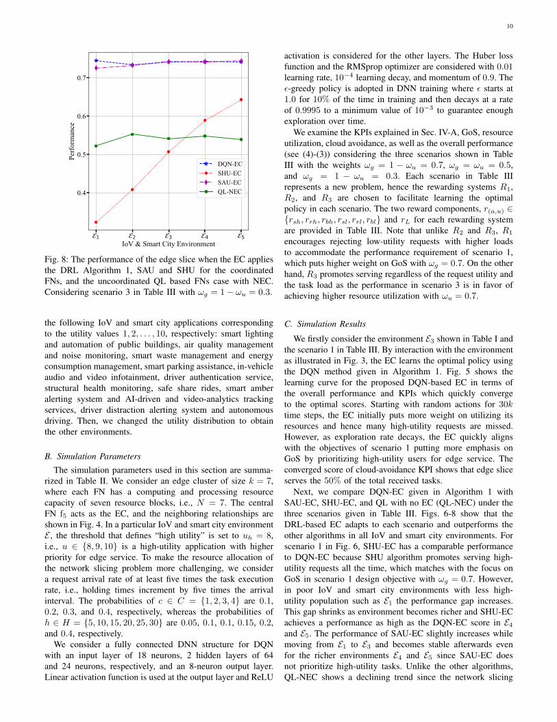
Fig. 8: The performance of the edge slice when the EC appliesthe DRL Algorithm 1, SAU and SHU for the coordinatedFNs, and the uncoordinated QL based FNs case with NEC.Considering scenario 3 in Table III with ωg = 1− ωu = 0.3.
the following IoV and smart city applications correspondingto the utility values 1, 2, . . . , 10, respectively: smart lightingand automation of public buildings, air quality managementand noise monitoring, smart waste management and energyconsumption management, smart parking assistance, in-vehicleaudio and video infotainment, driver authentication service,structural health monitoring, safe share rides, smart amberalerting system and AI-driven and video-analytics trackingservices, driver distraction alerting system and autonomousdriving. Then, we changed the utility distribution to obtainthe other environments.
B. Simulation Parameters
The simulation parameters used in this section are summa-rized in Table II. We consider an edge cluster of size k = 7,where each FN has a computing and processing resourcecapacity of seven resource blocks, i.e., N = 7. The centralFN f5 acts as the EC, and the neighboring relationships areshown in Fig. 4. In a particular IoV and smart city environmentE , the threshold that defines “high utility” is set to uh = 8,i.e., u ∈ {8, 9, 10} is a high-utility application with higherpriority for edge service. To make the resource allocation ofthe network slicing problem more challenging, we considera request arrival rate of at least five times the task executionrate, i.e., holding times increment by five times the arrivalinterval. The probabilities of c ∈ C = {1, 2, 3, 4} are 0.1,0.2, 0.3, and 0.4, respectively, whereas the probabilities ofh ∈ H = {5, 10, 15, 20, 25, 30} are 0.05, 0.1, 0.1, 0.15, 0.2,and 0.4, respectively.
We consider a fully connected DNN structure for DQNwith an input layer of 18 neurons, 2 hidden layers of 64and 24 neurons, respectively, and an 8-neuron output layer.Linear activation function is used at the output layer and ReLU
activation is considered for the other layers. The Huber lossfunction and the RMSprop optimizer are considered with 0.01learning rate, 10−4 learning decay, and momentum of 0.9. Theε-greedy policy is adopted in DNN training where ε starts at1.0 for 10% of the time in training and then decays at a rateof 0.9995 to a minimum value of 10−3 to guarantee enoughexploration over time.
We examine the KPIs explained in Sec. IV-A, GoS, resourceutilization, cloud avoidance, as well as the overall performance(see (4)-(3)) considering the three scenarios shown in TableIII with the weights ωg = 1 − ωu = 0.7, ωg = ωu = 0.5,and ωg = 1 − ωu = 0.3. Each scenario in Table IIIrepresents a new problem, hence the rewarding systems R1,R2, and R3 are chosen to facilitate learning the optimalpolicy in each scenario. The two reward components, r(a,u) ∈{rsh, rrh, rbh, rsl, rrl, rbl} and rL for each rewarding systemare provided in Table III. Note that unlike R2 and R3, R1
encourages rejecting low-utility requests with higher loadsto accommodate the performance requirement of scenario 1,which puts higher weight on GoS with ωg = 0.7. On the otherhand, R3 promotes serving regardless of the request utility andthe task load as the performance in scenario 3 is in favor ofachieving higher resource utilization with ωu = 0.7.
C. Simulation Results
We firstly consider the environment E3 shown in Table I andthe scenario 1 in Table III. By interaction with the environmentas illustrated in Fig. 3, the EC learns the optimal policy usingthe DQN method given in Algorithm 1. Fig. 5 shows thelearning curve for the proposed DQN-based EC in terms ofthe overall performance and KPIs which quickly convergeto the optimal scores. Starting with random actions for 30ktime steps, the EC initially puts more weight on utilizing itsresources and hence many high-utility requests are missed.However, as exploration rate decays, the EC quickly alignswith the objectives of scenario 1 putting more emphasis onGoS by prioritizing high-utility users for edge service. Theconverged score of cloud-avoidance KPI shows that edge sliceserves the 50% of the total received tasks.
Next, we compare DQN-EC given in Algorithm 1 withSAU-EC, SHU-EC, and QL with no EC (QL-NEC) under thethree scenarios given in Table III. Figs. 6-8 show that theDRL-based EC adapts to each scenario and outperforms theother algorithms in all IoV and smart city environments. Forscenario 1 in Fig. 6, SHU-EC has a comparable performanceto DQN-EC because SHU algorithm promotes serving high-utility requests all the time, which matches with the focus onGoS in scenario 1 design objective with ωg = 0.7. However,in poor IoV and smart city environments with less high-utility population such as E1 the performance gap increases.This gap shrinks as environment becomes richer and SHU-ECachieves a performance as high as the DQN-EC score in E4and E5. The performance of SAU-EC slightly increases whilemoving from E1 to E3 and becomes stable afterwards evenfor the richer environments E4 and E5 since SAU-EC doesnot prioritize high-utility tasks. Unlike the other algorithms,QL-NEC shows a declining trend since the network slicing

11
1 2 3 4 5IoV & Smart City Environment
0.0
0.2
0.4
0.6
0.8
1.0
KPI
Sco
re
GoSUtilizationCloud Avoidance
(a) DQN-EC, ωg = 0.7 and ωu = 0.3.
1 2 3 4 5IoV & Smart City Environment
0.0
0.2
0.4
0.6
0.8
1.0
KPI
Sco
re
GoSUtilizationCloud Avoidance
(b) DQN-EC, ωg = ωu = 0.5.
1 2 3 4 5IoV & Smart City Environment
0.0
0.2
0.4
0.6
0.8
1.0
KPI
Sco
re
GoSUtilizationCloud Avoidance
(c) DQN-EC, ωg = 0.3 and ωu = 0.7.
1 2 3 4 5IoV & Smart City Environment
0.0
0.2
0.4
0.6
0.8
1.0
KPI
Sco
re
GoSUtilizationCloud Avoidance
(d) SAU-EC, all scenarios.
1 2 3 4 5IoV & Smart City Environment
0.0
0.2
0.4
0.6
0.8
1.0
KPI
Sco
re
GoSUtilizationCloud Avoidance
(e) SHU-EC, all scenarios.
1 2 3 4 5IoV & Smart City Environment
0.0
0.2
0.4
0.6
0.8
1.0
KPI
Sco
re
GoSUtilizationCloud Avoidance
(f) QL-NEC, ωg = 0.7 and ωu = 0.3.
1 2 3 4 5IoV & Smart City Environment
0.0
0.2
0.4
0.6
0.8
1.0
KPI
Sco
re
GoSUtilizationCloud Avoidance
(g) QL-NEC, ωg = ωu = 0.5.
1 2 3 4 5IoV & Smart City Environment
0.0
0.2
0.4
0.6
0.8
1.0
KPI
Sco
re
GoSUtilizationCloud Avoidance
(h) QL-NEC, ωg = 0.3 and ωu = 0.7.
Fig. 9: The score of the main three individual KPIs, GoS, resource utilization, and cloud avoidance when the EC appliesAlgorithm 1, SAU and SHU for coordinated FNs, and the uncoordinated QL at FNs with no EC, under the 3 scenarios inTable III.
problem becomes more challenging with uncoordinated FNswhile moving towards richer environments in this scenario.Fig. 7 represents scenario 2 with equal weights for GoS andresource utilization, where SAU-EC is the second performingalgorithm following DQN-EC. With less importance for GoS,the performance of SHU-EC is as low as the QL-NEC in E1and although it grows while moving to richer environments,it does not reach a comparable level until E4 and E5. Theuncoordinated FNs with QL-NEC is more steady in scenario2. Fig. 8 shows the performances in scenario 3 in whichmore emphasis is put on resource utilization than GoS withωu = 0.7. It is observed that SHU-EC fails to achieve acomparable level of performance compared to DQN-EC whileSAU-EC does.
Fig. 9 provides the detailed KPI scores for GoS, resource
utilization and cloud avoidance for all algorithms consideringthe three design scenarios in all environments. DQN-ECalways adapts to the design objective and the IoV and smartcity environment. It maximizes GoS in scenario 1 as shownin Fig. 9a, balances GoS and utilization for scenario 2 asobserved in Fig. 9b, and promotes resource utilization forscenario 3 as shown in Fig. 9c. QL-NEC in Figs. 9f-9h tries tobehave similarly as it learns by interaction, but unfortunatelythe uncoordinated FNs in the edge slice cannot achieve that.Note that, DQN-EC learns the right balance between GoSand resource utilization in each scenario. For instance, eventhough SHU-EC is the second performing in Fig. 6 followingDQN-EC, it has lower utilization and cloud avoidance scores,i.e., less edge-slice contribution to handle service requests asshown in Fig. 9e. Similarly, SAU-EC is well-performing in
12
0 40 70 100 130 160Time (2 × 10³)
0.72
0.74
0.76
0.78
0.80
0.82
0.84
Perf
orm
ance
DQN-ECSHU-EC
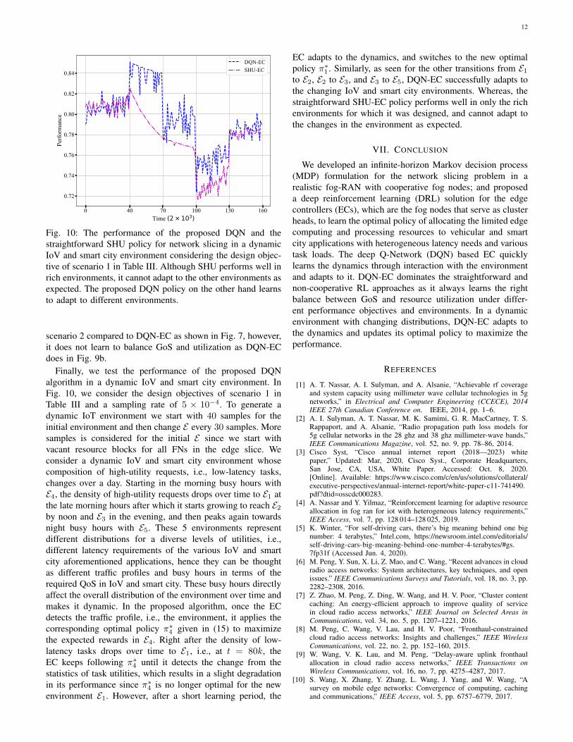
Fig. 10: The performance of the proposed DQN and thestraightforward SHU policy for network slicing in a dynamicIoV and smart city environment considering the design objec-tive of scenario 1 in Table III. Although SHU performs well inrich environments, it cannot adapt to the other environments asexpected. The proposed DQN policy on the other hand learnsto adapt to different environments.
scenario 2 compared to DQN-EC as shown in Fig. 7, however,it does not learn to balance GoS and utilization as DQN-ECdoes in Fig. 9b.
Finally, we test the performance of the proposed DQNalgorithm in a dynamic IoV and smart city environment. InFig. 10, we consider the design objectives of scenario 1 inTable III and a sampling rate of 5 × 10⁻⁴. To generate adynamic IoT environment we start with 40 samples for theinitial environment and then change E every 30 samples. Moresamples is considered for the initial E since we start withvacant resource blocks for all FNs in the edge slice. Weconsider a dynamic IoV and smart city environment whosecomposition of high-utility requests, i.e., low-latency tasks,changes over a day. Starting in the morning busy hours withE4, the density of high-utility requests drops over time to E1 atthe late morning hours after which it starts growing to reach E2by noon and E3 in the evening, and then peaks again towardsnight busy hours with E5. These 5 environments representdifferent distributions for a diverse levels of utilities, i.e.,different latency requirements of the various IoV and smartcity aforementioned applications, hence they can be thoughtas different traffic profiles and busy hours in terms of therequired QoS in IoV and smart city. These busy hours directlyaffect the overall distribution of the environment over time andmakes it dynamic. In the proposed algorithm, once the ECdetects the traffic profile, i.e., the environment, it applies thecorresponding optimal policy π∗4 given in (15) to maximizethe expected rewards in E4. Right after the density of low-latency tasks drops over time to E1, i.e., at t = 80k, theEC keeps following π∗4 until it detects the change from thestatistics of task utilities, which results in a slight degradationin its performance since π∗4 is no longer optimal for the newenvironment E1. However, after a short learning period, the
EC adapts to the dynamics, and switches to the new optimalpolicy π∗1 . Similarly, as seen for the other transitions from E1to E2, E2 to E3, and E3 to E5, DQN-EC successfully adapts tothe changing IoV and smart city environments. Whereas, thestraightforward SHU-EC policy performs well in only the richenvironments for which it was designed, and cannot adapt tothe changes in the environment as expected.
VII. CONCLUSION
We developed an infinite-horizon Markov decision process(MDP) formulation for the network slicing problem in arealistic fog-RAN with cooperative fog nodes; and proposeda deep reinforcement learning (DRL) solution for the edgecontrollers (ECs), which are the fog nodes that serve as clusterheads, to learn the optimal policy of allocating the limited edgecomputing and processing resources to vehicular and smartcity applications with heterogeneous latency needs and varioustask loads. The deep Q-Network (DQN) based EC quicklylearns the dynamics through interaction with the environmentand adapts to it. DQN-EC dominates the straightforward andnon-cooperative RL approaches as it always learns the rightbalance between GoS and resource utilization under differ-ent performance objectives and environments. In a dynamicenvironment with changing distributions, DQN-EC adapts tothe dynamics and updates its optimal policy to maximize theperformance.
REFERENCES
[1] A. T. Nassar, A. I. Sulyman, and A. Alsanie, “Achievable rf coverageand system capacity using millimeter wave cellular technologies in 5gnetworks,” in Electrical and Computer Engineering (CCECE), 2014IEEE 27th Canadian Conference on. IEEE, 2014, pp. 1–6.
[2] A. I. Sulyman, A. T. Nassar, M. K. Samimi, G. R. MacCartney, T. S.Rappaport, and A. Alsanie, “Radio propagation path loss models for5g cellular networks in the 28 ghz and 38 ghz millimeter-wave bands,”IEEE Communications Magazine, vol. 52, no. 9, pp. 78–86, 2014.
[3] Cisco Syst, “Cisco annual internet report (2018—2023) whitepaper,” Updated: Mar, 2020, Cisco Syst., Corporate Headquarters,San Jose, CA, USA, White Paper. Accessed: Oct. 8, 2020.[Online]. Available: https://www.cisco.com/c/en/us/solutions/collateral/executive-perspectives/annual-internet-report/white-paper-c11-741490.pdf?dtid=osscdc000283.
[4] A. Nassar and Y. Yilmaz, “Reinforcement learning for adaptive resourceallocation in fog ran for iot with heterogeneous latency requirements,”IEEE Access, vol. 7, pp. 128 014–128 025, 2019.
[5] K. Winter, “For self-driving cars, there’s big meaning behind one bignumber: 4 terabytes,” Intel.com, https://newsroom.intel.com/editorials/self-driving-cars-big-meaning-behind-one-number-4-terabytes/#gs.7fp31f (Accessed Jun. 4, 2020).
[6] M. Peng, Y. Sun, X. Li, Z. Mao, and C. Wang, “Recent advances in cloudradio access networks: System architectures, key techniques, and openissues.” IEEE Communications Surveys and Tutorials, vol. 18, no. 3, pp.2282–2308, 2016.
[7] Z. Zhao, M. Peng, Z. Ding, W. Wang, and H. V. Poor, “Cluster contentcaching: An energy-efficient approach to improve quality of servicein cloud radio access networks,” IEEE Journal on Selected Areas inCommunications, vol. 34, no. 5, pp. 1207–1221, 2016.
[8] M. Peng, C. Wang, V. Lau, and H. V. Poor, “Fronthaul-constrainedcloud radio access networks: Insights and challenges,” IEEE WirelessCommunications, vol. 22, no. 2, pp. 152–160, 2015.
[9] W. Wang, V. K. Lau, and M. Peng, “Delay-aware uplink fronthaulallocation in cloud radio access networks,” IEEE Transactions onWireless Communications, vol. 16, no. 7, pp. 4275–4287, 2017.
[10] S. Wang, X. Zhang, Y. Zhang, L. Wang, J. Yang, and W. Wang, “Asurvey on mobile edge networks: Convergence of computing, cachingand communications,” IEEE Access, vol. 5, pp. 6757–6779, 2017.

13
[11] Y.-Y. Shih, W.-H. Chung, A.-C. Pang, T.-C. Chiu, and H.-Y. Wei,“Enabling low-latency applications in fog-radio access networks,” IEEEnetwork, vol. 31, no. 1, pp. 52–58, 2017.
[12] S.-H. Park, O. Simeone, and S. Shamai, “Joint optimization of cloud andedge processing for fog radio access networks,” in Information Theory(ISIT), 2016 IEEE International Symposium on. IEEE, 2016, pp. 315–319.
[13] G. P. Fettweis, “The tactile internet: Applications and challenges,” IEEEVehicular Technology Magazine, vol. 9, no. 1, pp. 64–70, 2014.
[14] T. Lin, H. Rivano, and F. Le Mouel, “A survey of smart parkingsolutions,” IEEE Transactions on Intelligent Transportation Systems,vol. 18, no. 12, pp. 3229–3253, 2017.
[15] T. Anagnostopoulos, A. Zaslavsky, K. Kolomvatsos, A. Medvedev,P. Amirian, J. Morley, and S. Hadjieftymiades, “Challenges and op-portunities of waste management in iot-enabled smart cities: A survey,”IEEE Transactions on Sustainable Computing, vol. 2, no. 3, pp. 275–289, 2017.
[16] P. Barsocchi, P. Cassara, F. Mavilia, and D. Pellegrini, “Sensing acity’s state of health: Structural monitoring system by internet-of-thingswireless sensing devices,” IEEE Consumer Electronics Magazine, vol. 7,no. 2, pp. 22–31, 2018.
[17] Z. Hu, Z. Bai, K. Bian, T. Wang, and L. Song, “Real-time fine-grainedair quality sensing networks in smart city: Design, implementation, andoptimization,” IEEE Internet of Things Journal, vol. 6, no. 5, pp. 7526–7542, 2019.
[18] L. Ruge, B. Altakrouri, and A. Schrader, “Soundofthecity - continu-ous noise monitoring for a healthy city,” in 2013 IEEE InternationalConference on Pervasive Computing and Communications Workshops(PERCOM Workshops), 2013, pp. 670–675.
[19] P. T. Daely, H. T. Reda, G. B. Satrya, J. W. Kim, and S. Y. Shin,“Design of smart led streetlight system for smart city with web-basedmanagement system,” IEEE Sensors Journal, vol. 17, no. 18, pp. 6100–6110, 2017.
[20] M. Teliceanu, G. C. Lazaroiu, and V. Dumbrava, “Consumption profileoptimization in smart city vision,” in 2017 10th International Symposiumon Advanced Topics in Electrical Engineering (ATEE), 2017, pp. 876–881.
[21] F. Heimgaertner, S. Hettich, O. Kohlbacher, and M. Menth, “Scalinghome automation to public buildings: A distributed multiuser setup foropenhab 2,” in 2017 Global Internet of Things Summit (GIoTS), 2017,pp. 1–6.
[22] 3GPP, “Study on scenarios and requirements for next generation accesstechnologies (release 14), v14.2.0,” Mar., 2017, pp. 23-25. 3GPP, SophiaAntipolis, France, Rep. TR 38.913. Accessed: Oct. 8, 2020. [On-line]. Available: https://portal.3gpp.org/desktopmodules/Specifications/SpecificationDetails.aspx?specificationId=2996.
[23] G. J. Sutton, J. Zeng, R. P. Liu, W. Ni, D. N. Nguyen, B. A.Jayawickrama, X. Huang, M. Abolhasan, Z. Zhang, E. Dutkiewicz et al.,“Enabling technologies for ultra-reliable and low latency communica-tions: from phy and mac layer perspectives,” IEEE CommunicationsSurveys & Tutorials, vol. 21, no. 3, pp. 2488–2524, 2019.
[24] J. Wang, J. Liu, and N. Kato, “Networking and communications in au-tonomous driving: A survey,” IEEE Communications Surveys Tutorials,vol. 21, no. 2, pp. 1243–1274, 2019.
[25] P. Schulz, M. Matthe, H. Klessig, M. Simsek, G. Fettweis, J. Ansari,S. A. Ashraf, B. Almeroth, J. Voigt, I. Riedel et al., “Latency criticaliot applications in 5g: Perspective on the design of radio interface andnetwork architecture,” IEEE Communications Magazine, vol. 55, no. 2,pp. 70–78, 2017.
[26] R. H. Goudar and H. N. Megha, “Next generation intelligent trafficmanagement system and analysis for smart cities,” in 2017 InternationalConference On Smart Technologies For Smart Nation (SmartTechCon),2017, pp. 999–1003.
[27] L. Lin, X. Liao, H. Jin, and P. Li, “Computation offloading toward edgecomputing,” Proceedings of the IEEE, vol. 107, no. 8, pp. 1584–1607,2019.
[28] H. Xiang, W. Zhou, M. Daneshmand, and M. Peng, “Network slicingin fog radio access networks: Issues and challenges,” IEEE Communi-cations Magazine, vol. 55, no. 12, pp. 110–116, 2017.
[29] A. Nassar and Y. Yilmaz, “Dynamic network slicing for fog radio accessnetworks,” in 2019 IEEE Global Conference on Signal and InformationProcessing (GlobalSIP), 2019, pp. 1–5.
[30] I. Afolabi, T. Taleb, K. Samdanis, A. Ksentini, and H. Flinck, “Networkslicing and softwarization: A survey on principles, enabling technolo-gies, and solutions,” IEEE Communications Surveys & Tutorials, vol. 20,no. 3, pp. 2429–2453, 2018.
[31] T. Dang and M. Peng, “Delay-aware radio resource allocation opti-mization for network slicing in fog radio access networks,” in 2018IEEE International Conference on Communications Workshops (ICCWorkshops), 2018, pp. 1–6.
[32] L. Tang, X. Zhang, H. Xiang, Y. Sun, and M. Peng, “Joint resourceallocation and caching placement for network slicing in fog radioaccess networks,” in 2017 IEEE 18th International Workshop on SignalProcessing Advances in Wireless Communications (SPAWC). IEEE,2017, pp. 1–6.
[33] Y. Sun, M. Peng, S. Mao, and S. Yan, “Hierarchical radio resourceallocation for network slicing in fog radio access networks,” IEEETransactions on Vehicular Technology, 2019.
[34] V. N. Ha and L. B. Le, “End-to-end network slicing in virtualized ofdma-based cloud radio access networks,” IEEE Access, vol. 5, pp. 18 675–18 691, 2017.
[35] Y. L. Lee, J. Loo, T. C. Chuah, and L. Wang, “Dynamic networkslicing for multitenant heterogeneous cloud radio access networks,”IEEE Transactions on Wireless Communications, vol. 17, no. 4, pp.2146–2161, 2018.
[36] A. Nassar and Y. Yilmaz, “Resource allocation in fog ran for heteroge-neous iot environments based on reinforcement learning,” in ICC 2019 -2019 IEEE International Conference on Communications (ICC), 2019,pp. 1–6.
[37] Y. Shi, Y. E. Sagduyu, and T. Erpek, “Reinforcement learning fordynamic resource optimization in 5g radio access network slicing,” in2020 IEEE 25th International Workshop on Computer Aided Modelingand Design of Communication Links and Networks (CAMAD), 2020, pp.1–6.
[38] V. Mnih, K. Kavukcuoglu, D. Silver, A. A. Rusu, J. Veness, M. G.Bellemare, A. Graves, M. Riedmiller, A. K. Fidjeland, G. Ostrovskiet al., “Human-level control through deep reinforcement learning,”Nature, vol. 518, no. 7540, p. 529, 2015.
[39] R. Li, Z. Zhao, Q. Sun, C. I, C. Yang, X. Chen, M. Zhao, and H. Zhang,“Deep reinforcement learning for resource management in networkslicing,” IEEE Access, vol. 6, pp. 74 429–74 441, 2018.
[40] H. Xiang, S. Yan, and M. Peng, “A realization of fog-ran slicing viadeep reinforcement learning,” IEEE Transactions on Wireless Commu-nications, vol. 19, no. 4, pp. 2515–2527, 2020.
[41] Y. Hua, R. Li, Z. Zhao, X. Chen, and H. Zhang, “Gan-powereddeep distributional reinforcement learning for resource management innetwork slicing,” IEEE Journal on Selected Areas in Communications,vol. 38, no. 2, pp. 334–349, 2020.
[42] Y. Abiko, T. Saito, D. Ikeda, K. Ohta, T. Mizuno, and H. Mineno,“Flexible resource block allocation to multiple slices for radio accessnetwork slicing using deep reinforcement learning,” IEEE Access, vol. 8,pp. 68 183–68 198, 2020.
[43] S. de Bast, R. Torrea-Duran, A. Chiumento, S. Pollin, and H. Gacanin,“Deep reinforcement learning for dynamic network slicing in ieee 802.11networks,” in IEEE INFOCOM 2019 - IEEE Conference on ComputerCommunications Workshops (INFOCOM WKSHPS), 2019, pp. 264–269.
[44] G. Sun, Z. T. Gebrekidan, G. O. Boateng, D. Ayepah-Mensah, andW. Jiang, “Dynamic reservation and deep reinforcement learning basedautonomous resource slicing for virtualized radio access networks,”IEEE Access, vol. 7, pp. 45 758–45 772, 2019.
[45] R. Sutton, and A. BartoMack, Reinforcement Learning: An Introduction.Cambridge, MA, USA: MIT Press, 1998.