Deep Reinforcement Learning

1

Outline

1.  Overview of Reinforcement Learning 2.  Policy Search 3.  Policy Gradient and Gradient Estimators 4.  Q-prop: Sample Efficient Policy Gradient and an Off-policy Critic 5.  Model Based Planning in Discrete Action Space

Note: These slides largely derive from David Silver’s video lectures + slides

http://www0.cs.ucl.ac.uk/staff/d.silver/web/Teaching.html

2

Reinforcement Learning 101

Agent Entity interacting with its surroundings

Environment Surroundings in which the agent interacts with

State Representation of agent and environment configuration

Reward Measure of success for positive feedback

3

Reinforcement Learning 101

Policy Map of the agent’s actions given the state.

V(S)= Value Function

Expectation Value of the future reward given a specific policy, starting at state S(t)

Q = Action-Value Function

Expectation value of the future reward following a specific policy, after a specific action at a specific state.

Model Predicts what the environment will do next.

4

Policy Evaluation Run policy iteratively in environment while updating Q(a,s) or V(s), until convergence:

Model Based Evaluation Model Free Evalutation

Learn from experience (sampling). Greedy policy over V(s) requires model

Evaluation over action space:

Learn Model from experience (Supervised Learning). Learn Value function V(s) from model.

Pros: Efficiently learns model and can reason about model uncertainty Cons: two sources of error from model and approximated V(s)

5

Real World Model World (Map)

Model Based Model Free

6

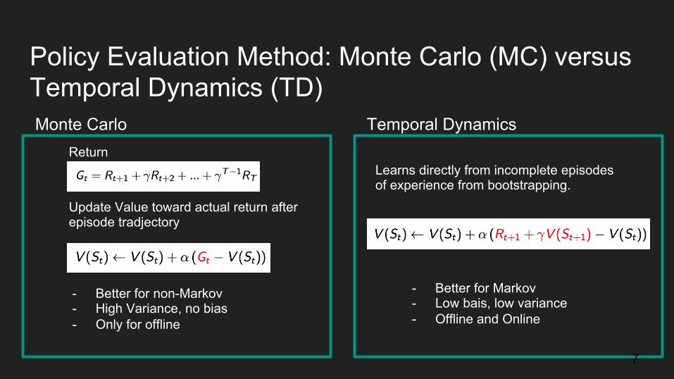
Policy Evaluation Method: Monte Carlo (MC) versus Temporal Dynamics (TD) Monte Carlo Temporal Dynamics

-  Better for non-Markov -  High Variance, no bias -  Only for offline

-  Better for Markov -  Low bais, low variance -  Offline and Online

Update Value toward actual return after episode tradjectory

Return Learns directly from incomplete episodes of experience from bootstrapping.

7

Policy Improvement

Update policy from the V(s) and/or Q(a,s) after iterated policy evalutation

Epsilon-Greedy

8

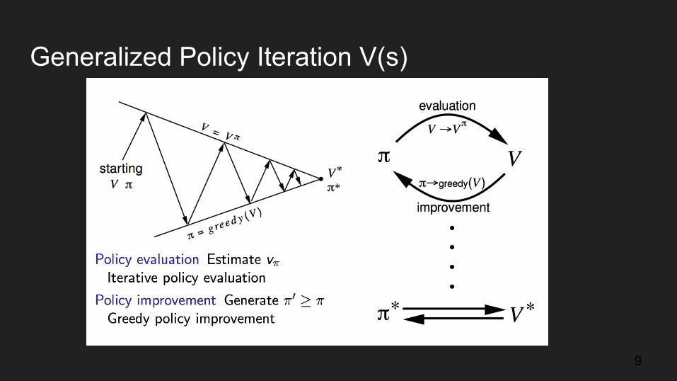
Generalized Policy Iteration V(s)

9

Generalized Policy Iteration Q(a,s)

10

Function Approximation for Large MDP Systems

Problem: Recall every state(s) has an entry V(s) and every action, state pair has an entry Q(a,s). This is problematic for large systems with many state pairs.

Solution: Estimate value function with approximation function. Generalize from seen states to unseen states and update parameter w using MC or TD learning.

11

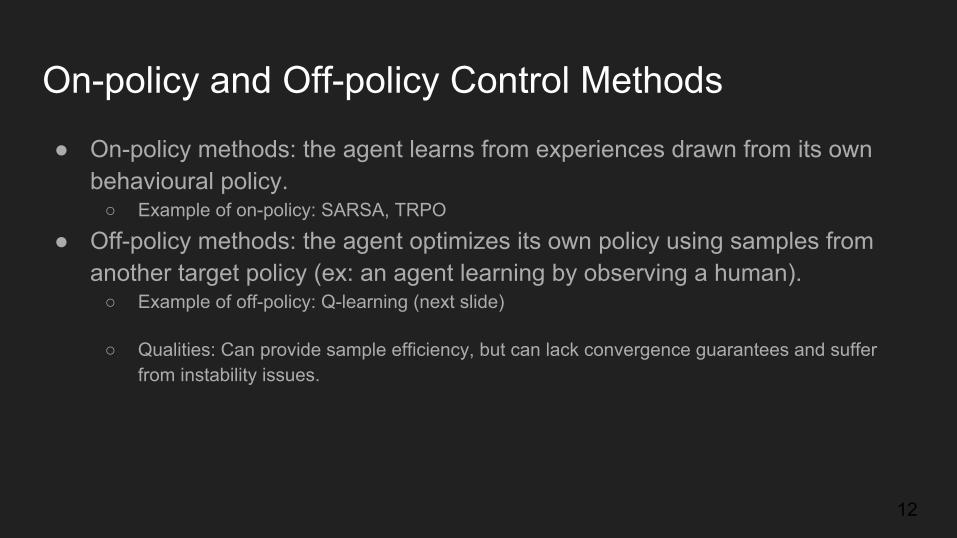
On-policy and Off-policy Control Methods

●  On-policy methods: the agent learns from experiences drawn from its own behavioural policy. ○  Example of on-policy: SARSA, TRPO

●  Off-policy methods: the agent optimizes its own policy using samples from another target policy (ex: an agent learning by observing a human). ○  Example of off-policy: Q-learning (next slide)

○  Qualities: Can provide sample efficiency, but can lack convergence guarantees and suffer from instability issues.

12

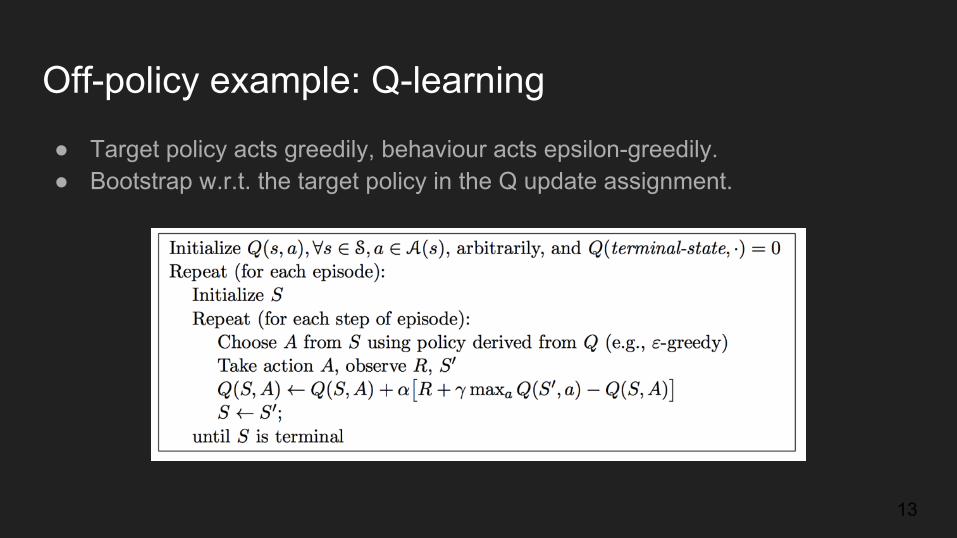
Off-policy example: Q-learning

●  Target policy acts greedily, behaviour acts epsilon-greedily. ●  Bootstrap w.r.t. the target policy in the Q update assignment.

13

Policy Gradient Methods Idea: Use function approximation on the policy:

Given its parameterization, we can directly optimize the policy. Take gradient of:

14

Policy Gradient Methods: Pros / Cons

Advantages:

●  Better convergence properties (updating tends to be smoother) ●  Effective in high-dimensional/cts action spaces (avoid working out max) ●  Can learn stochastic policies (more on this later)

Disadvantages:

●  Converge often to local minima ●  Can be inefficient to evaluate policy + have high variance (max operation can

be viewed as more aggressive)

15

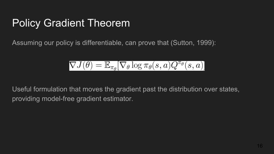
Policy Gradient Theorem

Assuming our policy is differentiable, can prove that (Sutton, 1999):

Useful formulation that moves the gradient past the distribution over states, providing model-free gradient estimator.

16

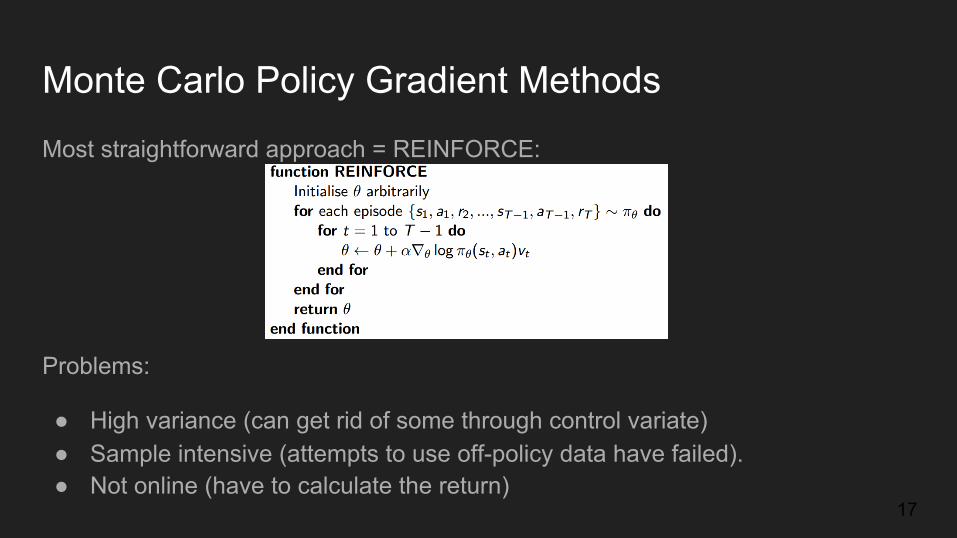
Monte Carlo Policy Gradient Methods

Most straightforward approach = REINFORCE:

Problems:

●  High variance (can get rid of some through control variate) ●  Sample intensive (attempts to use off-policy data have failed). ●  Not online (have to calculate the return)

17

Policy Gradient with Function Approximation

Approximate the gradient with a critic:

●  Employ techniques from before (e.g. Q-learning) to update Q. Off-policy techniques provide sample efficiency.

●  Can have reduced variance compared to REINFORCE (replacing full-step mc return with for example one-step TD return).

18

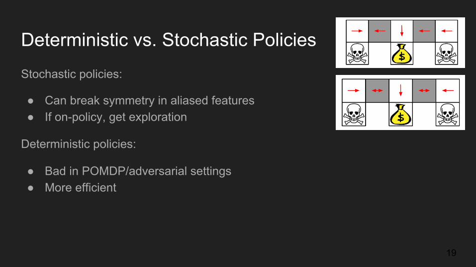
Deterministic vs. Stochastic Policies

Stochastic policies:

●  Can break symmetry in aliased features ●  If on-policy, get exploration

Deterministic policies:

●  Bad in POMDP/adversarial settings ●  More efficient

19

Why is deterministic more efficient?

●  Recall policy gradient theorem:

●  With stochastic policy gradient, the inner integral (red box in 2) is computed

by sampling a high dimensional action space. In contrast, the deterministic policy gradient can be computed immediately in closed form.

20

Q-Prop: Sample Efficient Policy Gradient with an Off-Policy Critic

Shixiang Gu, Timothy Lillicrap, Zoubin Ghahramani, Richard E. Turner, Sergey Levine

21

Q-Prop: Relevance

●  Challenges

○  On-policy estimators: sample efficiency, high variance with MC PG methods

○  Off-policy estimators: unstable results, non-convergence emanating from bias

●  Related Recent Work

○  Variance reduction in gradient estimators is an ongoing active research area..

○  Silver, Schulman etc. TRPO, DDPG

22

Q-Prop: Main Contributions

●  Q-prop provides a new approach for using off-policy data to reduce variance in an on-policy gradient estimator without introducing further bias.

●  Coalesce prior advances in dichotomous lines of research since Q-Prop uses

both on-policy updates and off-policy critic learning.

23

Q-Prop: Background ●  Monte Carlo (MC) Policy Gradient (PG) Methods:

●  PG with Function Approximation or Actor-Critic Methods

○  Policy evaluation step: fit a critic Q_w (using TD learning for e.g.) for the current policy π

○  Policy improvement step: optimize policy π against critic estimated Q_w

○  Significant gains in sample efficiency using off-policy (memory replay) TD learning for the critic ■  E.g. method: Deep Deterministic Policy Gradient (DDPG) [Silver et. al. 2014], used in Q-Prop

●  (Biased) Gradient (in policy improvement phase) given by:

24

Q-Prop: Estimator

25

Adaptive Q-Prop and Variants

26

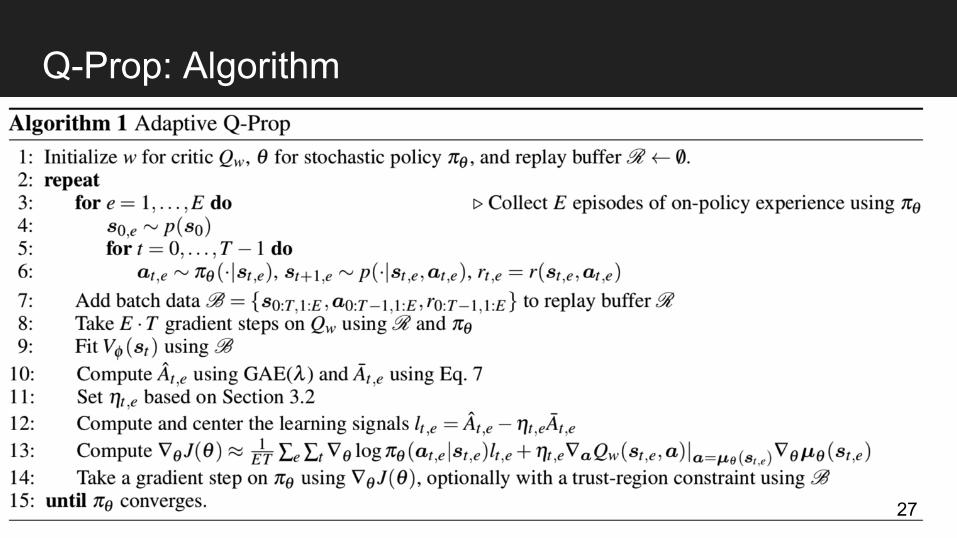
Q-Prop: Algorithm

27

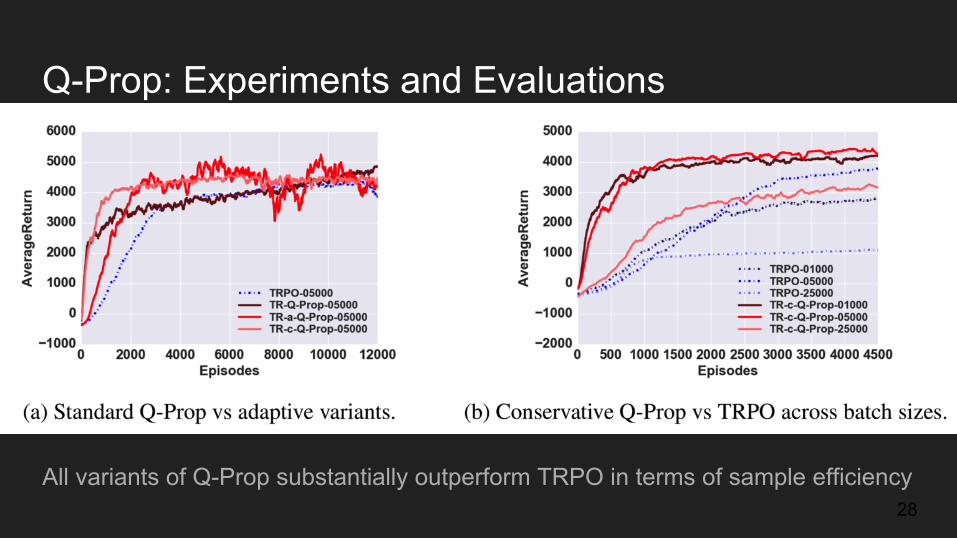
Q-Prop: Experiments and Evaluations

All variants of Q-Prop substantially outperform TRPO in terms of sample efficiency

28

Q-Prop: Evaluations Across Algorithms

TR-c-Q-Prop outperforms VPG, TRPO. DDPG is inconsistent (dependent on hyper-parameter settings (like reward scale – r – here)

29

Q-Prop: Evaluations Across Domains

Take away: Q-Prop often learns more sample efficiently than TRPO and can solve difficult domains such as Humanoid better than DDPG.

Q-Prop, TRPO and DDPG results showing the max average rewards attained in the first 30k episodes and the episodes to cross specific reward thresholds.

30

Q-Prop: Limitations

31

Q-Prop: Future Work

●  Q-Prop was implemented using TRPO-GAE for this paper. ●  Combining Q-Prop with other on-policy update schemes and off-policy critic

training methods is an interesting direction of future work.

32

Model-Based Planning in Discrete Action Spaces

By: Mikael Henaff, William F. Whitney, Yann LeCun

33

Model-based Reinforcement Learning

Recall: model-based RL uses a learned model of the world (i.e. how it changes as the agent acts).

The model can then be used to devise a way to get from a given state s0 to a desired state sf, via a sequence of actions.

This is in contrast to the model-free case, which learns directly from states and rewards.

Benefits:

-  Model reusability (e.g. can just change reward if task changes)

-  Better sample complexity (more informative error signal)

-  In continuous case, can optimize efficiently

34

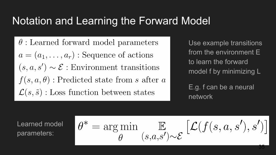
Notation and Learning the Forward Model

Use example transitions from the environment E to learn the forward model f by minimizing L

E.g. f can be a neural network

Learned model parameters:

35

Planning in Model-based Reinforcement Learning

Goal: given f, find the sequence of actions a that takes us from a starting state s0 to a desired final state sf

In the continuous case, this can be done via gradient descent in action space.

But what if the action space is discrete?

36

Problems in Discrete Action Spaces

-  It is too expensive to enumerate the tree of possibilities and find the optimal path (reminiscent of classical AI search e.g. in games)

-  If we treat A as a vector space and naively attempt continuous optimization, it is likely that the resulting action will be invalid, i.e. not an allowed action

Suppose our discrete space is one-hot encoded with dimension d

Can we somehow map this to a differentiable problem, more amenable to optimization?

37

Handling Discreteness (I): Overview

Two approaches are used to ameliorate the problems caused by discreteness:

1.  Softening the action space and relaxing the discrete optimization problem allows back-propagation to be used with gradient descent

2.  Biasing the algorithm to producing action vectors that are close to valid, by additive noise (implicit) or an entropy penalty (explicit)

38

Handling Discreteness (II): Soften & Relax

Define a new input space for the actions, defined by the d-dimensional simplex

Notice that we can get a softened action from any real vector by taking its softmax

Relaxing the optimization then gives (notice the x’s are not restricted):

Note: the softmax is applied element-wise 39

Handling Discreteness (III): Optimization Bias

The paper considers 3 ways to push the “input” xt’s towards one-hot vectors during the optimization procedure:

1.  Add noise to the input xt‘s 2.  Add noise to the gradients (scaled version of 1.) 3.  Add an explicit penalty to the loss function, given by the entropy of the

softened action H( sigma( xt ) )

This entropy is a good measure for how well this bias (or regularization) is working (since low entropy means furthest from uniform, i.e. more concentration at one value)

40

Why Does Adding Noise Help?

Adding noise to the inputs xt implicitly induces the following additional penalty to the optimization objective:

Also less sensitivity, by penalizing low loss but high curvature (e.g. sharp or unstable local minima)

Encourage less sensitivity to inputs (e.g. going to saturated softmax areas)

Noise variance (strength)

41

The Overall Planning Algorithm

42

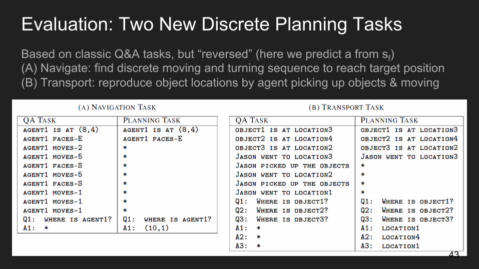
Evaluation: Two New Discrete Planning Tasks Based on classic Q&A tasks, but “reversed” (here we predict a from sf) (A) Navigate: find discrete moving and turning sequence to reach target position (B) Transport: reproduce object locations by agent picking up objects & moving

43

Results (I): Entropy and Loss over Time

Empirically, adding noise directly to the inputs seems to be the best of the 3 implicit loss regularization methods (possibly helps avoid local minima too)

One can also see that the entropy decreases over time, when regularization is present (right)

44

Results (II): Performance Comparison The method (the Forward Planner) was compared to Q-learning and an imitation learner. It does better at generalizing for longer sequences (outside training data) Issue: the Forward Planner takes much longer to choose (i.e. plan) its actions. But if even if given less time, it still performs reasonably well.

45

Summary of Paper

-  Devise a way to perform model-based planning in discrete actions spaces via gradient-based optimization

-  Combines: (1) relaxation of the problem and action space, and (2) a penalty that biases the algorithm naturally towards preferring low entropy (soft) actions

-  Defined two new discrete RL tasks and demonstrated their model’s state-of-the-art performance on them

46

Thank you

47

Appendix

48

REINFORCE

49

Related Theorems

●  Stochastic Policy Gradient Theorem [Sutton et. al., 1999] ●  Deterministic Policy Gradient Theorem [Silver et. al. 2015]

50

Open AI Gym MujoCo

●  Humanoid Demo

○  https://www.youtube.com/watch?v=SHLuf2ZBQSw

●  Half Cheetah

○  https://www.youtube.com/watch?v=EzBmQsiUWB

51

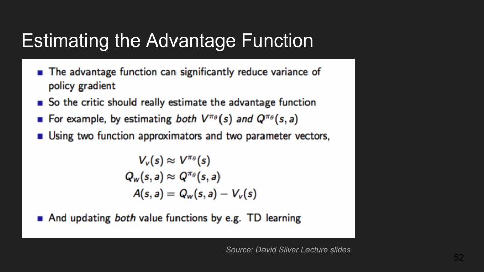
Estimating the Advantage Function

Source: David Silver Lecture slides 52

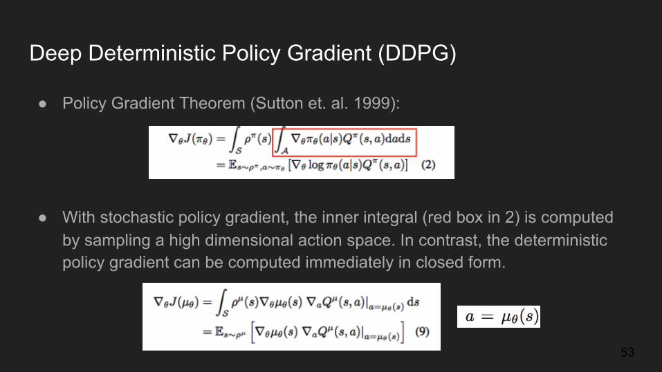
Deep Deterministic Policy Gradient (DDPG)

●  Policy Gradient Theorem (Sutton et. al. 1999):

●  With stochastic policy gradient, the inner integral (red box in 2) is computed

by sampling a high dimensional action space. In contrast, the deterministic policy gradient can be computed immediately in closed form.

53