arX

iv:1

801.

0573

3v2

[ph

ysic

s.co

mp-

ph]

7 F

eb 2

018

Deep Convolutional Neural Networks for Eigenvalue Problems in

Mechanics

David Finola, Yan Lua, Vijay Mahadevanb,1, Ankit Srivastavaa,∗

aDepartment of Mechanical, Materials, and Aerospace Engineering, Illinois Institute of Technology, Chicago, IL,

60616 USAbAmazon AWS AI Group

Abstract

In this paper we show that deep convolutional neural networks (CNN) can massively outper-form traditional densely connected neural networks (both deep or shallow) in predicting eigenvalueproblems in mechanics. In this sense, we strike out in a novel direction in mechanics computationswith strongly predictive neural networks whose success depends not only in neural architecturesbeing deep, but also in being fundamentally different from traditional neural architectures whichhave been used in mechanics until now. To show this, we consider a model problem: predicting theeigenvalues of a 1-D phononic crystal. However, the general observations pertaining to the predic-tive superiority of CNNs over fully-connected multi-layer perceptrons (MLP) should extend to otherproblems in mechanics as well. In the present problem, the optimal CNN architecture reaches 98%accuracy level on unseen data when optimized with just 40,000 samples. Fully-connected MLPs -typically the network of choice in mechanics research - on the other hand, does not improve beyond85% accuracy even with 100, 000 samples. We also show that even with a relatively small amount oftraining data, CNNs have the capability to generalize well for our problems and that they automat-ically learn deep symmetry operations such as translation invariance. Most importantly, however,we show how CNNs can naturally represent mechanical material tensors and that the convolutionoperation of CNNs has the ability to serve as local receptive fields which is a natural representationof mechanical response. Strategies proposed here may be used for other problems of mechanics andmay, in the future, be used to completely sidestep certain cumbersome algorithms with a purelydata driven approach based upon deep architectures of modern neural networks such as deep CNNs.

Keywords: Convolutional Neural Networks, Phononic crystal, Deep learning in Mechanics

1. Introduction

There has been a recent surge of interest in using deep learning using CNNs for machine learn-ing problems in the areas of speech recognition, image and natural language processing, whereadvanced pattern recognition is required in data which is generally arranged in grid-like topologies[1]. Beginning with image classification tasks, deep CNNs have consistently outperformed baseline

∗Corresponding authorEmail address: asriva13@iit.edu (Ankit Srivastava)

1Work done prior to joining Amazon

Preprint submitted to Computer Methods in Applied Mechanics and Engineering February 9, 2018

mathematical models with prediction accuracies in some tasks exceeding 98% [2]. In several areas,deep CNNs have achieved and even surpassed human level performance. For instance, in speechrecognition in particular the baseline approaches [3, 4, 5] have been completely outperformed bystatistical learning techniques, including CNN model architectures [6, 7]. The latter techniques haverecently reached human-level accuracy [8, 9]. This rise of the deep CNNs over the last half a decadehas been aided by a similar improvement in the computational capabilities which are required bysuch convolutional neural networks. Graphical Processing Units have proved particularly adept attraining very large CNNs using increasingly large amounts of available data[10].

All this raises an important question: can deep architectures, such as CNNs, also be usedto replace or aid certain mathematical computations central to the area of mechanics? To ourknowledge, this question has not been considered before by other researchers in the field. There hasadmittedly been a recent push towards purely data driven mechanics computing [11, 12, 13, 14, 15].However, these studies did not employ CNNs but other predictive tools such as regression andprincipal component analyses. There has also been a very recent push towards physics informedneural networks [16] as a way to make deep networks more data efficient but they also seem to limitto MLPs as their architecture. Similarly, authors have recently used deep networks for numericalquadrature calculations in FEM but have, again, limited the architecture to MLPs [17]. Moretraditionally, the mechanics community has been using MLPs for various pattern recognition tasksand computations for several decades now [18, 19, 20]. Furthermore, the neural networks whichhave been used have tended to be shallow in model depth characterized by a small number oflayers, a small number of nodes per layer and a single set of computational elements. In thisrespect, the neural network approaches of the mechanics community resemble the pre-CNN eraapproaches of the machine learning community. In the machine learning community, it has beenwell established that deep CNN models significantly overpower both shallow ones and deep MLPsdue to the following[21, 22, 23, 24]:

• Shallow networks show poorer generalization capabilities for highly nonlinear input-outputrelationships.

• Deep networks provide a more compact distributed representation of input output relation-ships.

A principal contribution of this paper is to develop some basic aspects of the framework whichwould allow deep CNNs to be employed for mechanics computations. Since no previous study existsin this domain, here we choose to focus on a simple eigenvalue problem in mechanics and trainnetworks of various architectures to predict its eigenvalues. We show that deep CNNs massivelyoutperform MLPs in this task. Another important contribution is to move from shallow networksin mechanics research to deep networks which are then efficiently trained over Graphical ProcessingUnits, thereby progressing towards achieving research parity with the more traditional areas ofmachine learning such as vision and speech recognition.

There are some key ideas that make CNNs particularly suitable for solving problems encounteredin the mechanics field. First, CNNs employ the concept of receptive fields in their core architectureexploiting spatially local correlation in grid-like topologies [25]. This implies that CNNs mayrepresent a powerful tool for pattern recognition in various computational mechanics and materialsproblems which are characterized by local interactions.

Second, there is a well-established consensus in the machine learning community that CNNsare efficiently able to learn representations which exhibit certain underlying symmetries [26, 27].

2

CNN architectures tend to be equivariant to general affine input transformations of the nature oftranslations, rotations and small distortions [28, 29]. Instinctively, therefore, we expect that CNNswould be naturally suited to mechanics problems which exhibit such symmetries. These include,but is not limited to, areas in mechanics which are built on symmetries such as the mechanics anddynamics of periodic structures.

Finally, unlike MLPs, CNNs allow for multiple channels to be associated with each input nodea feature that has been successfully exploited to represent the RGB channels of individual pixelsfor image recognition purposes. For problems in mechanics, the concept can be naturally extendedwhere the components of the material tensors of individual discretized elements can be identified asmultiple channels to individual nodes in a CNN. CNNs require minimal preprocessing to be able toclassify high-dimensional patterns from a complex decision surface [30]. Our aim with this paper is,then, to demonstrate the potential of CNNs in the field of computational mechanics by deployingdeep CNN architectures for a narrowly focused eigenvalue problem. We compare our results withresults from MLPs showing the massive performance boost that is possible with the use of CNNs.

2. Problem Description

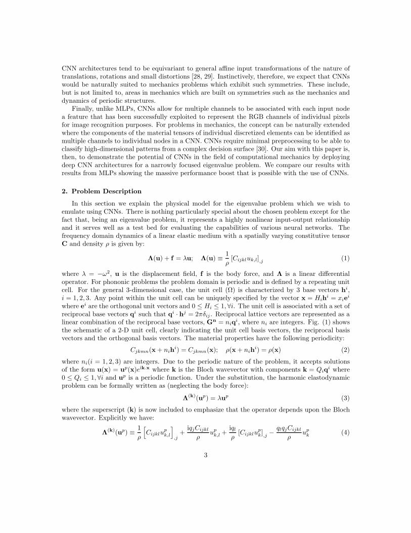
In this section we explain the physical model for the eigenvalue problem which we wish toemulate using CNNs. There is nothing particularly special about the chosen problem except for thefact that, being an eigenvalue problem, it represents a highly nonlinear input-output relationshipand it serves well as a test bed for evaluating the capabilities of various neural networks. Thefrequency domain dynamics of a linear elastic medium with a spatially varying constitutive tensorC and density ρ is given by:

Λ(u) + f = λu; Λ(u) ≡1

ρ[Cijkluk,l],j (1)

where λ = −ω2, u is the displacement field, f is the body force, and Λ is a linear differentialoperator. For phononic problems the problem domain is periodic and is defined by a repeating unitcell. For the general 3-dimensional case, the unit cell (Ω) is characterized by 3 base vectors hi,i = 1, 2, 3. Any point within the unit cell can be uniquely specified by the vector x = Hih

i = xiei

where ei are the orthogonal unit vectors and 0 ≤ Hi ≤ 1, ∀i. The unit cell is associated with a set ofreciprocal base vectors qi such that qi · hj = 2πδij . Reciprocal lattice vectors are represented as alinear combination of the reciprocal base vectors, Gn = niq

i, where ni are integers. Fig. (1) showsthe schematic of a 2-D unit cell, clearly indicating the unit cell basis vectors, the reciprocal basisvectors and the orthogonal basis vectors. The material properties have the following periodicity:

Cjkmn(x+ nihi) = Cjkmn(x); ρ(x+ nih

i) = ρ(x) (2)

where ni(i = 1, 2, 3) are integers. Due to the periodic nature of the problem, it accepts solutionsof the form u(x) = up(x)eik.x where k is the Bloch wavevector with components k = Qiq

i where0 ≤ Qi ≤ 1, ∀i and up is a periodic function. Under the substitution, the harmonic elastodynamicproblem can be formally written as (neglecting the body force):

Λ(k)(up) = λup (3)

where the superscript (k) is now included to emphasize that the operator depends upon the Blochwavevector. Explicitly we have:

Λ(k)(up) ≡1

ρ

[

Cijklupk,l

]

,j+

iqjCijkl

ρupk,l +

iqlρ

[Cijklupk],j −

qlqjCijkl

ρupk (4)

3

to zero, we arrive at the following system of linear homo-

s:

jk i ¼

mn i ¼

jk . For the general 3-dimen-

if to

in the

of the stress tensor, these coefficients

of of

jk

To approximate the stress and displacement fields in

, we use test functions of the following form:

Þ ¼ Þ

of the test functions

In order for the test functions to be suitable they should

, and should be orthog-

in the sense mentioned above. To show that these test

we note for

¼ ð jk

Þ ¼ Þ ð jkÞÞ bd Þ

10

we

Þ ¼ 11

To show orthogonality we note that

i ¼ Þ Þ

½ð þð þð Þ

12

of the test functions.

of the test functions

A special note of consideration here regards the spatial

of the test function. The set of linear homoge-

of the test functions in

It is, therefore, neces-

to express the test functions in these coordinates. To

do this we first express in the reciprocal basis

) and in the unit cell basis ( ) and by

ij we note that,

Þ ¼ ½ð þð þð 13

d in the orthogonal coordinate

is theth

in the orthogonal coordinate system and is theth

of the vector in this system. By taking a dot prod-

of this equation with the three orthogonal unit vectors

we can express in terms of

¼ ½ ½ f 14

3 matrix jk

be written as,

Þ ¼ 15

11 Þ þ 12 Þ þ 13

21 Þ þ 22 Þ þ 23

31 Þ þ 32 Þ þ 33 16

thof the test function is now given by:

¼ ð kj 17

3. Numerical solution

of the composite is given by the

to nontrivial solutions of . To cal-

is first written in the following

HS

18

1. of a 2-dimensional periodic composite. The unit cell vectors ( ), reciprocal basis vectors ( ), and the orthogonal vectors (

A. Srivastava, S. Nemat-Nasser /Mechanics of Materials 74 (2014) 67–75 69

Figure 1: Schematic of a 2-dimensional periodic composite. The unit cell vectors (h1,h2), reciprocal basis vectors

(q1,q2), and the orthogonal vectors (e1, e2) are shown.

For a suitable span of the wavevector, the sets of eigenvalues λn (and the corresponding frequenciesωn) constitute the phononic dispersion relation of the composite. There are several numericaltechniques for calculating the eigenvalues but a common method is to expand the field variableup in an appropriate basis and then use the basis to convert the differential equation into a set oflinear equations. Both the Plane Wave Expansion[31] method and Rayleigh quotient[32] follow thisstrategy.

2.1. 1-D

There is only one possible Bravais lattice in 1-dimension with a unit cell vector whose lengthequals the length of the unit cell itself (Fig. 2a). Without any loss of generality we take the directionof this vector to be the same as e1. If the length of the unit cell is a, then we have h1 = ae1. Thereciprocal vector is given by q1 = (2π/a)e1. The wave-vector of a Bloch wave traveling in thiscomposite is specified as k = Q1q

1. To completely characterize the band-structure of the unit cellit is sufficient to evaluate the dispersion relation in the irreducible Brillouin zone (0 ≤ Q1 ≤ .5). Forplane longitudinal wave propagating in the e1 direction the only displacement component of interestis u1 and the only relevant stress component is σ11. The equation of motion and the constitutivelaw are:

σ11,1 = −λρ(x1)u1; σ11 = E(x1)u1,1 (5)

where E(x1) is the spatially varying Young’s modulus. The exact dispersion relation for 1-Dlongitudinal wave propagation in a periodic layered composite can be solved using the transfermatrix method [33]. For 2-phase composites, the relation is particulary simple [34],

cos(ka) = cos(ωh1/c1) cos(ωh2/c2)− Γ sin(ωh1/c1) sin(ωh2/c2),

Γ = (1 + κ2)/(2κ), κ = ρ1c1/(ρ2c2), (6)

where hi is the thickness, ρi is the density, and ci is the longitudinal wave velocity of the ith layer(i = 1, 2) in a unit cell. We can solve for the corresponding wave number k (or, equivalently, Q1)by providing a frequency, ω (or, equivalently, f = ω/2π), using (6). These f −Q1 (or ω − k) pairsconstitute the eigenvalue band-structure of the composite when the wavevector is made to span thefirst Brillouin zone (Q1 ∈ [0, 0.5]). A representative example of the bandstructure, calculated fora representative 1-D, 2-phase composite (Fig. 2a), is shown in Fig. (2b). The frequency values in

4

e1 h1 q1 h1

Phase 1 Phase 2 Phase 1

0 0.1 0.2 0.3 0.4 0.5

Q1

0

1

2

3

4

5

6

7

Fre

qu

en

cy H

z

105

a b

Figure 2: a. Schematic of a 1-dimensional 2-phased periodic composite. The unit cell vector (h1), reciprocal basisvector (q1), and the orthogonal vector (e1) are shown, b. Bandstructure of a 1-D, 2-phase phononic crystal showingthe frequency eigenvalues constituting the first two passbands. Unit cell details in [33].

Fig. (2b) are, thus, related to the eigenvalues of the phononic crystal when a certain wavenumberQ1 is specified. Results in Fig. (2) are calculated by using the exact physical solution of the systemgiven by the Rytov equation (6). Our aim in this paper is to train neural networks of varyingarchitectures to sidestep the physical model as represented by Eqs. (5,6).

2.2. Input-output relationship framework

The phononic eigenvalue problem described above can be represented as an input-output rela-tionship. Formally, we can write:

e = fc(E(x1), ρ(x1), Q1) (7)

where e is a vector of eigenvalues which is obtained through a vector of nonlinear functions fc whichoperates on the space dependent material properties (E, ρ) and a choice of the wavenumber Q1.An approximation to the eigenvalues can be generated by considering the material properties asdiscretely defined over the unit cell. We first normalize the unit cell with its length and discretize therange of x1 (x1 ∈ [0, 1]) into N segments. We identify the material properties over these segmentsas the input variables. The material properties now become vectors themselves, individually definedover each segment, and the input-output relationship becomes:

e = fd(E,ρ, Q1), E = Ei,ρ = ρi; i = 1, 2...N (8)

where fd are the sought approximations to the continuous input-output relationships fc in (7). Inthis paper we have taken N = 100 and we have sought to train neural networks to learn and predictfd from a set of training data. The training data consists of input and output datasets createdfrom the solution of the exact problem (5,6,7). Specifically, the input data consists of randomlygenerated instantiations of vectors E,ρ and the output data consists of the corresponding firsttwo eigenvalues, appropriately normalized, at chosen values of Q1. For the set of problems underconsideration, we seek to estimate the first two eigenvalues at 10 different Q1 points within therange of Q1 ([0,0.5]). This essentially translates into an output vector size of 20 and a flat input

5

vector size of 200. 100 elements of the input vector correspond to E and the rest correspond toρ. In training neural networks to learn this input output relationships, there are some questions ofprimary concern. Some of these pertain to the architecture of the network, the number of trainingdata needed to achieve a certain desired error, the method of training the network, the methodby which the training data is generated, and the effect of the training data on the ability of thenetwork to generalize for unseen examples. These are discussed in detail in the next sections.

3. Neural Networks and the Representation Learning Approach

A central problem in mechanics, as in other areas, is the approximation of a function whichrelates an input to an output in a system of interest (7). The traditional method of attempting thisproblem is to manually convert the inputs to a set of representative features which could then berelated to the outputs. Representation learning, on the other hand, is a set of techniques that allowsa system to automatically discover the representations needed for feature detection, classification orreal-value mapping from raw data. This replaces manual feature engineering and allows a machineto both learn the features and use them to perform a specific task (Fig. 3). Neural networksare a set of algorithms which perform this task of representation learning by creating automaticrepresentations of input data in their hidden layers. The first precursors to the modern neuralnetworks were proposed by Rosenblatt [35]. Since then, significant advances in the area of machinelearning has led to modern neural networks with complex function approximation capabilities [10].Artificial Neural Networks (ANN) are comprised of multiple interconnected simple computationalelements called neurons. Both the fully-connected multi-layer perceptrons and convolutional neuralnetworks fit within the class of ANNs and they differ primarily in their neuronal architecture andinterconnectivity.

Figure 3: Manual feature crafting vs. the representation learning approach

3.1. Multi-Layer Perceptrons

The Multi-layer Perceptron (MLP) concept, more generally referred as feed-forward neural net-work, was initially proposed as an universal function approximator [36]. The objective of an MLPis to approximate a function f between inputs x and outputs y:

y = f(x) (9)

6

This process can be represented in NN terms as a function mapping of inputs to the outputsthrough a set of optimizable parameters. For the single hidden layer MLP shown in Fig. (4), theseoptimization parameters are the weight matrices V,W and the mapping is approximated as:

y ≈ f(x, θ) = Wg(Vx) (10)

where appropriate matrix multiplications are assumed. g represents the activation function whichis generally a non-linear transformation. The weights of the network are typically stochasticallyinitiated and are subsequently tuned within the training phase of the network. One method oftraining the network is to relate its known input-output data and minimize its prediction deviationfrom the output by appropriately changing the weights, through an optimization process.

!"#

$%&'( )*+

,-.

/01

234

56789:;<

=>?

@ABCDEF

GHI

JKLMNOPQR

STU

VWX YZ[\]^_`a bcdefghij

klmnopqrs

tuvwxyz|~

Figure 4: Graph of a simple Multi-layer Perceptron with fully-connected layers

3.2. Convolutional Neural Networks

Three key ideas differentiate convolutional networks from conventional networks, which havemade them highly successful in various engineering and science fields [37, 38, 39, 40, 41, 42, 43]: the use of convolution operation, the implementation of the Rectified Linear (ReLU) activationfunction, and a representation-invariance imposing operation termed Pooling.

3.2.1. Convolution

An important difference between a fully connected MLP and a CNN is the use of the convolutionoperation instead of the standard matrix multiplication operation. So while in the case of theMLP in Fig. (4), the inputs to the neurons in the middle layer are obtained by a simple matrixmultiplication of the weight V and the input x, for a CNN, the input will instead be transformedusing a convolution operation through a kernel w into a feature map h. Assuming that the inputis a 2-D vector of length N and depth d, this can be represented as a 3-D matrix of size N × 1× d.The kernel is similarly assumed to be a matrix of size m× 1 × d where m < N . In this case, oneelement of the feature map will be calculated by computing the Einstein sum hl = xj+l,1,kwj,1,k; j =1, ...m, k = 1, ...d where l is the current location of the filter. The filter is then advanced from itscurrent location by a predetermined step size termed stride and the next element of the featuremap is calculated. In our examples presented below, a good value of the stride is determined to

7

be 1. This process is repeated until the kernel spans x in the length dimension and completes thecalculation of h. This process is symbolically represented as:

h = x ∗w (11)

where ∗ represents the convolution operation. In our 1D phononic eigenvalue problem, the inputsare the spatially ordered sequence of material property values. These are represented by an inputvector X whose depth is 2. In the depthwise direction, the first element corresponds to the modulusof a given finite element and the second element corresponds to the density value. The convolutionallayer, for our case, convolves each input matrix with k kernels wi resulting in a total of k featuremaps. Each feature map hi is computed as follows:

hi = X ∗wi + bi, i = 1, ..., k. (12)

where bi are bias parameters. CNNs work by tuning the parameters of the kernels wi and the biasparameters bi in order to learn the desired input-output relationships. There are some interestingpoints to note here. First, the feature maps corresponding to the modulus and density channels arenot completely independent of each other as they are generated from the dot product of the samekernel wi. This allows the neural network to associate the different material properties at a pointas belonging to the same material. Second, the concepts of kernels allows for the feature mapsto represent local interactions. This sparsity allows CNNs to learn an input-output relationshipdependent upon spatial and temporal structure more efficiently than MLPs.

3.2.2. ReLU Activation

Having calculated the pre-activation feature maps hi, they are passed through nonlinear acti-vation functions commonly referred to as ReLU. The Rectifier Linear Unit Rectifier Linear Unit(ReLU) [44] has proven to provide high computational efficiency and is a piece-wise linear activationfunction that outputs zero if the input is negative and outputs the input if it is greater than zero.Mathematically, given a feature map hi, a ReLU function is defined as follows:

hi = max(0,hi) (13)

in which hi and hi represent the ReLU input and output respectively.

3.2.3. Pooling Operation

Once the convolution operations have been applied along with ReLU activations, the outputspass through a parameter-reducing layer commonly referred to as a max-pooling layer. The outputof this layer is the maximum unit from p adjacent input units. In our 1-D problem, poolingis performed along both the transformed modulus and density data axes (Fig. 5.) Following thefindings of optimal CNN achitectures in computer vision and speech recognition [45, 46] and our ownoptimization work, the pooling operation is performed only once in our case, after two consecutiveconvolution layers. The general intuition is that as more pooling layers are applied, units in higherlayers would be less discriminative with respect to the variations in input features [47].

3.3. Optimization Algorithm

For both MLPs and CNNs in this paper, we employed the Stochastic Gradient Descent withMomemtum (SGDM) through backpropagation optimization algorithm for network training. The

8

Figure 5: Convolution and max-pooling transformations of modulus and density axes

training is performed on small groups of data-sets, termed mini-batches, at a time. The algorithmupdates the model parameter by taking small steps in the direction of negative gradient:

θl+1 = θl − α∇E(θl) + γ(θl − θl−1) (14)

where θl represents the optimizable model parameters at iteration l, α is the learning rate, E(θl) isthe current minibatch cost function and the γ(θl−θl−1) is the contribution of the previous gradientstep to the current iteration [48]. The specific algorithm employed is termed as Adam and it involvesadaptive learning rates for different parameters from estimates of first and second moments of thegradients [49].

3.4. Objective Function

Hung et al and Lippmann [50, 51] have demonstrated that neural networks based on squared-error functions are able to accurately estimate posterior probabilities for finite sample sizes. Themean squared error objective function is defined as,

MSE =1

m

∑

(y − y)2

(15)

where y is the prediction and y is the actual target output (eigenvalue in our case.) The summationis over all outputs and over all the data points in a mini-batch and m is the total number of termsin the summation.

3.5. Data Mapping and Normalization

As is standard practice in neural networks, all input material property data is normalizedthrough mean normalization:

xnorm =x− x

xmax − xmin(16)

where x is the mean of the input vector. Furthermore, the eigenvalues are also normalized by areference maximum, as is standard practice in the machine learning field.

9

4. Numerical Experiments

4.1. Data Generation

The input data for the CNN described above was generated following standard physical princi-ples that guide the phononic eigenvalue problem as previously described. The training, validation,and test data sets can be divided into two broad categories. In the first category, the materialproperty vectors E and ρ were generated using a uniform probability distribution on the modulusand density values. The probability distribution was created with lower and upper bounds for boththe modulus (lower bound: 100MPa, upper bound: 300GPa) and density (lower bound: 800kg/m3,upper bound: 8000kg/m3). From these distributions, we created 100-element unit cells Ωi randomlygenerated , which are characterized by modulus vectors Ei and density vectors ρi. Correspondingto these unit cells, we calculated the 20 eigenvalues of interest which constitute the output datavectors ei. This dataset category is termed Dataset-A for future reference and has a total of 300,000data samples. In the respective results, a small fraction of this dataset was employed purely formodel tranining, validation and, in an initial phase, testing of the networks. We note that since themodulus and density values in Dataset-A are independently sampled from two different probabilitydistributions, the material properties assigned to the individual elements in any given Ωi very likelydo not correspond to any real material.

The second broad category of data used in this paper is aimed at testing specific capabilities ofthe model in making predictions for those unit cells Ω which might be of more practical interestbut which are highly unlikely to be represented in Dataset-A. One such example is the case whereΩ is composed of only 2 different material phases - a configuration which appears frequently inthe phononics and metamaterial literature [33, 52]. To create a dataset corresponding to thisconfiguration, we divided the 100-element unit cell into two zones of 50 elements each. All elementsin these individual zones were then assigned randomly generated but same modulus and densityvalues. The input-output data for this dataset is referred to as Dataset-2. We similarly createddatasets for 3 and 10 material phases and refer to them as Dataset-3 and Dataset-10 respectivelywhich, in addition to Dataset-2, is collectively referred to as Dataset-B. At this point it should benoted that it is highly unlikely that any individual case appearing in Dataset-B also appears inDataset-A.

4.2. Model Architectures

After an iterative process of line search in the hyperparameters of the CNNs employed, it wasdetermined that a good model for our phononic eigenvalue problem has the following architecture:There are 100 input nodes corresponding to the 100-element unit cell (Fig. 6). Each input nodehas two channels with individual channels corresponding to the density and modulus values of theelement. This is a crucial piece of information in our CNN implementation in that we choose toidentify the various material properties of an element with individual channels in a CNN. Not onlydoes this create a direct correspondence with the practice of identifying the RGB information ata pixel with individual channels in computer vision applications, it also guides how CNNs couldbe employed for problems in mechanics in higher dimensions. In higher dimensions, more materialproperties (components of elasticity tensor) are required to describe the behavior of materials.Given the success of CNNs in our current 1-D problem, a promising strategy going forward wouldbe to identify these material properties as different channels in a CNN input node layer.

Following the input node is a set of two convolution layers with ReLU activation functions.The convolution filters has a size of 3 in the dimension of the input vector. A max-pooling layer

10

¡

¢£¤¥¦§¨© ª«¬­®¯°± ²³´µ¶·¸¹ º»¼½¾ ¿ÀÁÂÃÄÅ

ÆÇÈÉÊËÌÍÎÏÐÑÒÓÔÕÖ

×ØÙÚÛÜÝÞßàáâãäåæçèéêëìíîï

ðñòóô

õö÷øùúûüýþÿ

!"#$%&'(

)*+,-./0123 456789

:;<=>?@A BCDEFGHIJKL MNO

PQRSTUV WX

Y

Z

Figure 6: CNN architecture used for the study

follows the set of convolution layers with a filter dimension of 2×1. These layers are followed by twofully connected dense layers with ReLU activation functions. Subsequently, a fully connected layerwith linear or Gaussian connections leads to the outputs of the network which are the eigenvaluesof the problem. This CNN architecture has more than 7 million optimizable parameters. For thepurposes of most of the results shown below, it was trained on 28,000 samples which took a little lessthan 13 minutes on a GPU (NVIDIA GTX980). Once the network is trained, prediction obviouslytakes a much smaller amount of time (fraction of a second.) The same input-output mapping wasalso performed using a multi-layer perceptron with only fully connected layers, which was used togenerate some of the key results presented in this paper. The architecture that yielded the bestprediction accuracy was found to have 6 hidden layers with 1024 computational units in each layer(Fig. 7.) The final output layer consisted of gaussian or linear connections to the output units.

[\]^_`ab cdefghijklm no p

qrstu

vwxyz|~

¡¢£¤

¥¦§¨©ª

«¬­®

¯°±²³´µ¶·¸ ¹º»¼½¾

¿À

ÁÂÃÄ

Å

Æ

Figure 7: MLP architecture used for the study

11

4.3. Results

4.3.1. Approximation Capabilities of CNNs

Our initial focus was on obtaining average eigenvalue prediction accuracies higher than 95%on unseen examples and comparing the performance of CNNs vs regular MLPs in achieving thismetric. We define mean absolute accuracy of our predictions:

e = 1−1

p

∑ |(y − y)|

y(17)

where the summation is being carried out over all eigenvalues and all test data and p is the totalnumber of terms in the summation. The error is then expressed as a percentage. For the purpose ofcomparison, we considered Dataset-A for training, validation, and testing purposes. As mentionedearlier, Dataset-A has 300,000 data samples. A randomly selected portion of these is used fortraining the networks and the rest of the unseen examples are used for validation and testingpurposes.

2 3 4 5 6 7 8 9 10

Number of Training Examples 104

0

5

10

15

20

25

30

Lowest Mean Absolute Error (%)

CNNFully-Connected MLP (Conventional NNs)

Figure 8: Comparison of prediction accuracy as a function of training data size (CNN vs MLP). NOTE: The numberof examples (horizontal axis) represent the size of the entire optimization set (Training+Validation+Testing)

The striking point about this comparison is that the CNN easily outperforms the MLP interms of eigenvalue prediction accuracy as can be seen in Fig. (8). Both networks improve intheir prediction accuracies as they are trained on larger fractions of Dataset-A. However, the CNNalready has a higher than 95% prediction accuracy when it has been trained only on 20,000 samples.At this level of training, the MLP has an accuracy of slighly greater than 70%. In fact, the MLPonly reaches about 85% accuracy at 100,000 training samples at which point the CNN is alreadyabove 98% prediction accuracy. The 30,000-40,000 samples range seems to be a breaking pointwhere both networks show the largest percental decrease of mean absolute error. In summary,these comparisons show that CNNs have the potential to achieve high prediction accuracies inproblems of mechanics with a fraction of the training data required by MLPs.

The CNN architecture employed was eventually able to achieve 1.13 % of mean absolute error inits eigenvalue predictions with a normalized 1-σ error of 2.11e-05. The small value of the standarddeviation shows that most of the distribution of prediction errors is heavily centered around its meanvalue. In other words, a large fraction of the predictions have absolute errors close to the reported

12

-20-18-16-14-12-10 -8 -6 -4 -2 0 2 4 6 8 10 12 14 16 18 20

Prediction Error (%)

0

1

2

3

4

5

Number of Instances

104

Error Distribution

Zero-Error Line

(a) Prediction error distribution

0 1000 2000 3000 4000 5000

Analytically Computed Eigenvalues

0

500

1000

1500

2000

2500

3000

3500

4000

4500

5000

Network Output Eigenvalues

Output = 1*Target + 0.28

Output = Prediction

Fit (R = 0.99975)

Data

(b) Regression of the targets relative to the output

1 2 3 4 5 6 7 8 9 10

Eigenvalue Label

0

500

1000

1500

2000

2500

Eigenvalue

Analytically Computed EigenvalueCNN Predicted Eigenvalue

(c) Representative eigenvalue outputs for a 2-phasesample

Figure 9: CNN Performance

mean of the distribution, whereas only a small fraction of the predictions has larger predictionerrors. Fig. (9b) shows all the predicted eigenvalues along with the associated analytically computedeigenvalues and clarifies the high correlation which exists between the two sets. This correlationcan be measured in terms of the Pearson correlation coefficient which, for the present case, is at thelevel of 0.999 indicating that the regression between the two sets is strongly linear. This can alsobe seen from the distribution of prediction errors in Fig. (9a) which shows that a vast majority ofthe predictions have errors in the ±2% range. Fig. (9c) shows an example prediction of the CNNcompared with actual eigenvalue calculations for a specific unseen phononic crystal configuration,which represents a sample from Dataset-2. Specifically, this sample represents a 2-phase materialwith two equal phases. One phase has a density of 5.80 g/cm3 and a modulus of 76.27 GPa andthe other phase has a density of 7.23 g/cm3 and a modulus of 23.61 GPa. It can then be seen thatall the 20 eigenvalues have been predicted with good accuracy by the CNN.

4.3.2. Generalization Capabilities of CNNs

From the previous section, it is evident that CNNs can massively outperform MLPs with fullyconnected layers in terms of their prediction accuracies for comparable training datasets. Another

13

(a) Distribution of Input Material Properties forDataset-A (100,000 samples)

(b) Distribution of Input Material Properties forDataset-2 (100,000 samples)

Figure 10: Comparison of the distribution on input material properties per element. Color map projection of thehistograms is shown on the lower part, with the lightest color representing the most instances.

important consideration in evaluating the efficacy of any approximating method is its capability togeneralize to unseen examples. To a limited extent, we have already shown that the trained CNNachieves very high prediction accuracies on unseen test data when the test data is extracted fromthe same distribution as the training and validation datasets. Here we consider the ability of theCNN to generalize to examples which are derived from distinctly different distributions. For this weconsider Dataset-A, Dataset-2, Dataset-3, and Dataset-10 as described earlier. While each of theelements in the samples in Dataset-A have materials properties that come from a random uniformdistribution, the rest of the datasets used in this section contains contrasting phases that naturallyyields a broader range of eigenvalue distributions. Representative 3D histograms for Dataset-A andDataset-2 can be seen in Fig. (10). The colormap projection in Fig. (10a) shows that there islargely an even distribution of samples spanning the property ranges for Dataset-A. For dataset-2(10b), the distribution is less even and it misses some density ranges that are present in Dataset-A.Most importantly, however, since Dataset-B corresponds to only 2-phase cases, its correspondingeigenvalue ranges are very different from those of the samples in Dataset-A. This is clarified in Fig.(11) which shows histogram plots of all the eigenvalues for Dataset-A, Dataset-2, and Dataset-10.It shows that the eigenvalue range spanned by Dataset-2 is about twice as large as that spannedby Dataset-A.

Fig. (11) shows some results which underline the generalization capabilities of the employedCNNs. First, when the network is only trained on Dataset-A, it is able to achieve < 16% predictionerrors on Dataset-2, < 15% prediction errors on Dataset-3, and < 13% prediction errors on Dataset-10 (blue bars.) This is interesting because not only does any input configuration in Dataset-2,Dataset-3, and Dataset-10 most likely does not exist in Dataset-A, there exist large eigenvalueranges in these datasets which the trained network was never trained on and has never seen. Theseprediction errors come down substantially when Dataset-A is augmented with some samples fromDataset-2 and Dataset-3 for training purposes. The results are shown by orange bars in Fig. (11).In this case, the prediction errors for Dataset-2, Dataset-3, and Dataset-10 are all below 6%. Note

14

Figure 11: Uniform sample from the N100 and the 2 real materials datasets, regarding the 1st upper eigenvalue fromthe band structure

that in this case, although the network was never trained on Dataset-10, it was able to generalizewell when tested on this dataset. From these results, there is strong indication that deep CNNsapplied as we present seem to be able to successfully generalize on completely new regions of theinput-output space, improving upon the typical issues brought by implementations of shallow andless diverse networks in mechanics. These deep networks also seem to require much less data toachieve and surpass the performance of traditional MLPs.

10-Phase Mat.

2-Phase Mat.

3-Phase Mat.

Dataset-A

Testing Dataset Category

0

2

4

6

8

10

12

14

16

Mean Absolute Error (%)

Training with Dataset-A onlyTraining with Dataset-A (50%), Dataset-2 (25%) and Dataset-3 (25%)

Figure 12: Model Generalization

4.3.3. Automatic learning of translational invariance

An important and interesting feature of our CNN implementation is that it seems to havelearned translational invariance of our problems automatically. Since phononic crystals are periodiccomposites, their eigenvalues (Eq. 3) are invariant under unit cell translations. In effect, it meansthat a 2-phase unit cell with a 50-50 distribution of the two material phases (P1 − P2) will have

15

the same eigenvalues as a 3 phase unit cell made by periodically translating the two materialsphases. For the latter, let’s consider as an example, a unit cell made of phases P1 − P2 − P1 witha 25-50-25 distribution respectively. Our CNN predicts practically the same eigenvalues for thetwo cases (both unseen), showing that it has learned translational invariance of the problem, Adeeper understanding of this can be done by reconstructing the activations of the deeper layers ofthe network and understanding the filter activations when a prediction is being made. For the mostpart, it is often not a trivial task to try to reconstruct the deeper layers of the network into theinput space. However, a simple activation analysis on the maxpooling layer is performed in thisstudy. The activations of the maxpooling filters feed directly to the regression layers and if thoseactivations are same in two cases then the network prediction will also be the same. In theory andif the network’s optimization is done successfully, filters should specialize such that their uniqueand sparse activation leads to the best output prediction possible. This means that input sampleswith similar input-output mappings would activate the same filters, while keeping the rest inactive.Fig. (13) shows the maxpooling filter activation results when the network is presented with three

0 50 100 150

Filter Number (Label)

0

0.05

0.1

0.15

0.2

Mean Filter Activation Value

Dataset-2 Sample (50-50)Dataset-2 Sample (25-50-25)Dataset-10

Figure 13: Mean post-pooling filter activations versus filter number for two symmetric samples from Dataset-2 (whichyields the same eigenvalue output) and a Dataset-10 sample

different input unit cells. Two of these (from Dataset-2) are physically the same, differing only witha translation and the third one is different as it is taken from Dataset-10. We notice from this figurethat for the cases of the translationally equivalent unit cells, not only are the same filters activatedbut their activation values are also practically the same. On the other hand, for the sample fromDataset-10, the filter activations differ not only in their values but also in which filters are activated.

4.4. Conclusion

We have shown that key mathematical properties that have made modern deep neural networkarchitectures, such as CNNs which have proven to be very successful in typical machine learning

16

implementation fields, can translate to complex input-output mapping tasks in mechanics. Throughour results, not only were we able to demonstrate that CNNs can successfully approximate thecomplex function mapping the material tensors of a phononic crystal to its eigenvalues, but alsothat it can be done with much better data efficiency and higher performance than when usingtraditional neural networks (densely connected MLPs). The CNN model architectures used in thisstudy present a much more diverse set of computational elements and deeper graph depth thataid both the feature abstraction process and the function approximation capabilities, as is wellestablished in the machine learning literature. The basic filter activation study in this paper alsoprovided a hint at how the feature abstraction and function mapping occurs in our implementation,leaving the door open for more a comprehensive study in future applications. We found that whenusing an optimized network to predict a case with a characteristic input translation that leads tothe same output, exactly the same post-pooling filters are consistently activated with and withpractically the same activation values. This fact provides clues that these filters are specializing incharacteristic input patterns that seems to be aiding the prediction of the output eigenvalues. Thisprocess has been noted to occur in computer vision applications of deep CNNs and have provenuseful in our application in mechanics as well.

There are many interesting questions worth pursuing after this study. The primary one isthe extension of this process to higher dimensions for the prediction of eigenvalues in more com-plex mechanics problems. In higher dimensions more material properties would need to be takeninto account. For instance, even if we consider an isotropic material, its mechanical descriptionwould generally require 3 independent constants (shear modulus, bulk modulus, and density). Foranisotropic materials this number further goes up. However, within the CNN framework presentedin this paper, taking these into account merely requires the addition of more channels or depth tothe input vectors. With this framework, it would be interesting to see if deep CNNs can be effi-ciently trained to act as substitutes for eigenvalue algorithms in the case of 2-, and 3-D mechanicsproblems. Such networks would have no fundamental computational complexity limitations withwhich all eigenvalue algorithms suffer and, therefore, would provide a way to explore design spaceswhich have not be probed yet. The idea of representing the elements of material property tensors asdifferent channels in a CNN, as proposed in this paper, is clearly not limited to eigenvalue problems.Therefore, it is conceivable that CNNs can similarly lead to significant improvements in regressionand classification tasks in non-eigenvalue mechanics problems including time domain problems.

Acknowledgements

A.S. acknowledges support from the NSF CAREER grant # 1554033 to the Illinois Institute ofTechnology.

References

References

[1] W. Rawat, Z. Wang, Deep convolutional neural networks for image classification: A compre-hensive review, Neural Computation.

[2] Y. LeCun, The mnist database of handwritten digits, http://yann. lecun. com/exdb/mnist/.

17

[3] L. R. Bahl, F. Jelinek, R. L. Mercer, A maximum likelihood approach to continuous speechrecognition, in: Readings in speech recognition, Elsevier, 1990, pp. 308–319.

[4] L. Bahl, P. Brown, P. De Souza, R. Mercer, Maximum mutual information estimation of hiddenmarkov model parameters for speech recognition, in: Acoustics, Speech, and Signal Processing,IEEE International Conference on ICASSP’86., Vol. 11, IEEE, 1986, pp. 49–52.

[5] S. E. Levinson, L. R. Rabiner, M. M. Sondhi, An introduction to the application of the theoryof probabilistic functions of a markov process to automatic speech recognition, The Bell SystemTechnical Journal 62 (4) (1983) 1035–1074.

[6] G. Hinton, L. Deng, D. Yu, G. E. Dahl, A.-r. Mohamed, N. Jaitly, A. Senior, V. Vanhoucke,P. Nguyen, T. N. Sainath, et al., Deep neural networks for acoustic modeling in speech recog-nition: The shared views of four research groups, IEEE Signal Processing Magazine 29 (6)(2012) 82–97.

[7] L. Deng, J. Li, J.-T. Huang, K. Yao, D. Yu, F. Seide, M. Seltzer, G. Zweig, X. He, J. Williams,et al., Recent advances in deep learning for speech research at microsoft, in: Acoustics, Speechand Signal Processing (ICASSP), 2013 IEEE International Conference on, IEEE, 2013, pp.8604–8608.

[8] W. Xiong, L. Wu, F. Alleva, J. Droppo, X. Huang, A. Stolcke,The microsoft 2017 conversational speech recognition system, CoRR abs/1708.06073.arXiv:1708.06073.URL http://arxiv.org/abs/1708.06073

[9] A. Stolcke, J. Droppo, Comparing human and machine errors in conversational speech tran-scription, arXiv preprint arXiv:1708.08615.

[10] J. Schmidhuber, Deep learning in neural networks: An overview, Neural networks 61 (2015)85–117.

[11] T. Kirchdoerfer, M. Ortiz, Data-driven computational mechanics, Computer Methods in Ap-plied Mechanics and Engineering 304 (2016) 81–101.

[12] T. Kirchdoerfer, M. Ortiz, Data driven computing with noisy material data sets, arXiv preprintarXiv:1702.01574.

[13] R. Ibanez, E. Abisset-Chavanne, J. V. Aguado, D. Gonzalez, E. Cueto, F. Chinesta, A man-ifold learning approach to data-driven computational elasticity and inelasticity, Archives ofComputational Methods in Engineering 25 (1) (2018) 47–57.

[14] A. Mosavi, T. Rabczuk, A. R. Varkonyi-Koczy, Reviewing the novel machine learning tools formaterials design, in: International Conference on Global Research and Education, Springer,2017, pp. 50–58.

[15] M. Bessa, R. Bostanabad, Z. Liu, A. Hu, D. W. Apley, C. Brinson, W. Chen, W. K. Liu,A framework for data-driven analysis of materials under uncertainty: Countering the curse ofdimensionality, Computer Methods in Applied Mechanics and Engineering 320 (2017) 633–667.

18

[16] A. Karpatne, W. Watkins, J. Read, V. Kumar, Physics-guided neural networks (pgnn): Anapplication in lake temperature modeling, arXiv preprint arXiv:1710.11431.

[17] A. Oishi, G. Yagawa, Computational mechanics enhanced by deep learning, Computer Methodsin Applied Mechanics and Engineering 327 (2017) 327–351.

[18] Z. Su, L. Ye, An intelligent signal processing and pattern recognition technique for defectidentification using an active sensor network, Smart materials and structures 13 (4) (2004)957.

[19] R. Challis, U. Bork, P. Todd, Ultrasonic nde of adhered t-joints using lamb waves and intelligentsignal processing, Ultrasonics 34 (2-5) (1996) 455–459.

[20] S. Legendre, D. Massicotte, J. Goyette, T. K. Bose, Neural classification of lamb wave ultrasonicweld testing signals using wavelet coefficients, IEEE Transactions on Instrumentation andMeasurement 50 (3) (2001) 672–678.

[21] Y. Bengio, et al., Learning deep architectures for ai, Foundations and trends R© in MachineLearning 2 (1) (2009) 1–127.

[22] O. Delalleau, Y. Bengio, Shallow vs. deep sum-product networks, in: Advances in NeuralInformation Processing Systems, 2011, pp. 666–674.

[23] R. Pascanu, G. Montufar, Y. Bengio, On the number of response regions of deep feed forwardnetworks with piece-wise linear activations, arXiv preprint arXiv:1312.6098.

[24] G. F. Montufar, R. Pascanu, K. Cho, Y. Bengio, On the number of linear regions of deepneural networks, in: Advances in neural information processing systems, 2014, pp. 2924–2932.

[25] I. Goodfellow, Y. Bengio, A. Courville, Deep learning, MIT press, 2016.

[26] R. Gens, P. M. Domingos, Deep symmetry networks, in: Advances in neural informationprocessing systems, 2014, pp. 2537–2545.

[27] M. Jaderberg, K. Simonyan, A. Zisserman, et al., Spatial transformer networks, in: Advancesin Neural Information Processing Systems, 2015, pp. 2017–2025.

[28] Y. LeCun, Learning invariant feature hierarchies, in: Computer vision–ECCV 2012. Workshopsand demonstrations, Springer, 2012, pp. 496–505.

[29] K. Lenc, A. Vedaldi, Understanding image representations by measuring their equivarianceand equivalence, in: Proceedings of the IEEE conference on computer vision and patternrecognition, 2015, pp. 991–999.

[30] Y. LeCun, et al., Lenet-5, convolutional neural networks, URL: http://yann. lecun.com/exdb/lenet.

[31] M. Kushwaha, P. Halevi, L. Dobrzynski, B. Djafari-Rouhani, Acoustic band structure of peri-odic elastic composites, Physical Review Letters 71 (13) (1993) 2022–2025.

[32] Y. Lu, A. Srivastava, Variational methods for phononic calculations, Wave Motion 60 (2016)46–61.

19

[33] A. Srivastava, Metamaterial properties of periodic laminates, Journal of the Mechanics andPhysics of Solids 96 (2016) 252–263.

[34] S. Rytov, Acoustical properties of a thinly laminated medium, Soviet Physics-Acoustics 2(1956) 68.

[35] F. Rosenblatt, The perceptron: A probabilistic model for information storage and organizationin the brain., Psychological review 65 (6) (1958) 386.

[36] K. Hornik, Approximation capabilities of multilayer feedforward networks, Neural networks4 (2) (1991) 251–257.

[37] S. Ji, W. Xu, M. Yang, K. Yu, 3d convolutional neural networks for human action recognition,IEEE transactions on pattern analysis and machine intelligence 35 (1) (2013) 221–231.

[38] P. Sermanet, D. Eigen, X. Zhang, M. Mathieu, R. Fergus, Y. LeCun, Overfeat: Inte-grated recognition, localization and detection using convolutional networks, arXiv preprintarXiv:1312.6229.

[39] M. Bojarski, D. Del Testa, D. Dworakowski, B. Firner, B. Flepp, P. Goyal, L. D. Jackel,M. Monfort, U. Muller, J. Zhang, et al., End to end learning for self-driving cars, arXivpreprint arXiv:1604.07316.

[40] A. Aurisano, A. Radovic, D. Rocco, A. Himmel, M. Messier, E. Niner, G. Pawloski, F. Psi-has, A. Sousa, P. Vahle, A convolutional neural network neutrino event classifier, Journal ofInstrumentation 11 (09) (2016) P09001.

[41] I. Wallach, M. Dzamba, A. Heifets, Atomnet: a deep convolutional neural network for bioac-tivity prediction in structure-based drug discovery, arXiv preprint arXiv:1510.02855.

[42] N. Tajbakhsh, J. Y. Shin, S. R. Gurudu, R. T. Hurst, C. B. Kendall, M. B. Gotway, J. Liang,Convolutional neural networks for medical image analysis: Full training or fine tuning?, IEEEtransactions on medical imaging 35 (5) (2016) 1299–1312.

[43] G. B. Goh, N. O. Hodas, A. Vishnu, Deep learning for computational chemistry, Journal ofComputational Chemistry.

[44] X. Glorot, A. Bordes, Y. Bengio, Deep sparse rectifier neural networks, in: Proceedings of theFourteenth International Conference on Artificial Intelligence and Statistics, 2011, pp. 315–323.

[45] Y. LeCun, Y. Bengio, et al., Convolutional networks for images, speech, and time series, Thehandbook of brain theory and neural networks 3361 (10) (1995) 1995.

[46] A. Krizhevsky, I. Sutskever, G. E. Hinton, Imagenet classification with deep convolutionalneural networks, in: Advances in neural information processing systems, 2012, pp. 1097–1105.

[47] Y. Zhang, M. Pezeshki, P. Brakel, S. Zhang, C. L. Y. Bengio, A. Courville, Towards end-to-endspeech recognition with deep convolutional neural networks, arXiv preprint arXiv:1701.02720.

[48] C. M. Bishop, Pattern recognition and machine learning, springer, 2006.

20

[49] D. Kingma, J. Ba, Adam: A method for stochastic optimization, arXiv preprintarXiv:1412.6980.

[50] M. Hung, M. Hu, M. Shanker, B. Patuwo, Estimating posterior probabilities in classifica-tion problems with neural networks, International Journal of Computational Intelligence andOrganizations 1 (1) (1996) 49–60.

[51] M. D. Richard, R. P. Lippmann, Neural network classifiers estimate bayesian a posterioriprobabilities, Neural computation 3 (4) (1991) 461–483.

[52] A. Srivastava, J. R. Willis, Evanescent wave boundary layers in metamaterials and sidesteppingthem through a variational approach, in: Proc. R. Soc. A, Vol. 473, The Royal Society, 2017,p. 20160765.

21