Deeper Insights into Graph Convolutional Networksfor Semi-Supervised Learning

Qimai Li1, Zhichao Han12, Xiao-Ming Wu1∗1The Hong Kong Polytechnic University

2ETH Zurichcsqmli@comp.polyu.edu.hk, zhhan@student.ethz.ch, xiao-ming.wu@polyu.edu.hk

AbstractMany interesting problems in machine learning are beingrevisited with new deep learning tools. For graph-based semi-supervised learning, a recent important development is graphconvolutional networks (GCNs), which nicely integrate localvertex features and graph topology in the convolutional lay-ers. Although the GCN model compares favorably with otherstate-of-the-art methods, its mechanisms are not clear and itstill requires considerable amount of labeled data for valida-tion and model selection.In this paper, we develop deeper insights into the GCN modeland address its fundamental limits. First, we show that thegraph convolution of the GCN model is actually a specialform of Laplacian smoothing, which is the key reason whyGCNs work, but it also brings potential concerns of over-smoothing with many convolutional layers. Second, to over-come the limits of the GCN model with shallow architectures,we propose both co-training and self-training approaches totrain GCNs. Our approaches significantly improve GCNs inlearning with very few labels, and exempt them from requir-ing additional labels for validation. Extensive experiments onbenchmarks have verified our theory and proposals.

1 IntroductionThe breakthroughs in deep learning have led to a paradigmshift in artificial intelligence and machine learning. On theone hand, numerous old problems have been revisited withdeep neural networks and huge progress has been made inmany tasks previously seemed out of reach, such as machinetranslation and computer vision. On the other hand, newtechniques such as geometric deep learning (Bronstein et al.2017) are being developed to generalize deep neural modelsto new or non-traditional domains.

It is well known that training a deep neural model typi-cally requires a large amount of labeled data, which cannotbe satisfied in many scenarios due to the high cost of labelingtraining data. To reduce the amount of data needed for train-ing, a recent surge of research interest has focused on few-shot learning (Lake, Salakhutdinov, and Tenenbaum 2015;Rezende et al. 2016) – to learn a classification model withvery few examples from each class. Closely related to few-shot learning is semi-supervised learning, where a large

∗Corresponding author.Copyright c© 2018, Association for the Advancement of ArtificialIntelligence (www.aaai.org). All rights reserved.

amount of unlabeled data can be utilized to train with typi-cally a small amount of labeled data.

Many researches have shown that leveraging unlabeleddata in training can improve learning accuracy significantlyif used properly (Zhu and Goldberg 2009). The key issue isto maximize the effective utilization of structural and fea-ture information of unlabeled data. Due to the powerful fea-ture extraction capability and recent success of deep neu-ral networks, there have been some successful attempts torevisit semi-supervised learning with neural-network-basedmodels, including ladder network (Rasmus et al. 2015),semi-supervised embedding (Weston et al. 2008), planetoid(Yang, Cohen, and Salakhutdinov 2016), and graph convo-lutional networks (Kipf and Welling 2017).

The recently developed graph convolutional neural net-works (GCNNs) (Defferrard, Bresson, and Vandergheynst2016) is a successful attempt of generalizing the power-ful convolutional neural networks (CNNs) in dealing withEuclidean data to modeling graph-structured data. In theirpilot work (Kipf and Welling 2017), Kipf and Welling pro-posed a simplified type of GCNNs, called graph convolu-tional networks (GCNs), and applied it to semi-supervisedclassification. The GCN model naturally integrates the con-nectivity patterns and feature attributes of graph-structureddata, and outperforms many state-of-the-art methods signif-icantly on some benchmarks. Nevertheless, it suffers fromsimilar problems faced by other neural-network-based mod-els. The working mechanisms of the GCN model for semi-supervised learning are not clear, and the training of GCNsstill requires considerable amount of labeled data for param-eter tuning and model selection, which defeats the purposefor semi-supervised learning.

In this paper, we demystify the GCN model for semi-supervised learning. In particular, we show that the graphconvolution of the GCN model is simply a special form ofLaplacian smoothing, which mixes the features of a vertexand its nearby neighbors. The smoothing operation makesthe features of vertices in the same cluster similar, thusgreatly easing the classification task, which is the key rea-son why GCNs work so well. However, it also brings poten-tial concerns of over-smoothing. If a GCN is deep withmany convolutional layers, the output features may be over-smoothed and vertices from different clusters may becomeindistinguishable. The mixing happens quickly on small

arX

iv:1

801.

0760

6v1

[cs

.LG

] 2

2 Ja

n 20

18

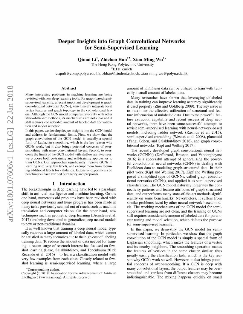
Figure 1: Performance comparison of GCNs, label propaga-tion, and our method for semi-supervised classification onthe Cora citation network.

datasets with only a few convolutional layers, as illustratedby Fig. 2. Also, adding more layers to a GCN will make itmuch more difficult to train.

However, a shallow GCN model such as the two-layerGCN used in (Kipf and Welling 2017) has its own limits.Besides that it requires many additional labels for validation,it also suffers from the localized nature of the convolutionalfilter. When only few labels are given, a shallow GCN cannoteffectively propagate the labels to the entire data graph. Asillustrated in Fig. 1, the performance of GCNs drops quicklyas the training size shrinks, even for the one with 500 addi-tional labels for validation.

To overcome the limits and realize the full potentials ofthe GCN model, we propose a co-training approach and aself-training approach to train GCNs. By co-training a GCNwith a random walk model, the latter could complement theformer in exploring global graph topology. By self-training aGCN, we can exploit its feature extraction capability to over-come its localized nature. Combining both the co-trainingand self-training approaches can substantially improve theGCN model for semi-supervised learning with very fewlabels, and exempt it from requiring additional labeled datafor validation. As illustrated in Fig. 1, our method outper-forms GCNs by a large margin.

In a nutshell, the key innovations of this paper are: 1)providing new insights and analysis of the GCN model forsemi-supervised learning; 2) proposing solutions to improvethe GCN model for semi-supervised learning. The rest ofthe paper is organized as follows. Section 2 introduces thepreliminaries and related works. In Section 3, we analyzethe mechanisms and fundamental limits of the GCN modelfor semi-supervised learning. In Section 4, we propose ourmethods to improve the GCN model. In Section 5, weconduct experiments to verify our analysis and proposals.Finally, Section 6 concludes the paper.

2 Preliminaries and Related WorksFirst, let us define some notations used throughout thispaper. A graph is represented by G = (V, E), where Vis the vertex set with |V| = n and E is the edge set.In this paper, we consider undirected graphs. Denote byA = [aij ] ∈ Rn×n the adjacency matrix which is nonnega-tive. Denote by D = diag(d1, d2, . . . , dn) the degree matrix

of A where di =∑j aij is the degree of vertex i. The graph

Laplacian (Chung 1997) is defined as L := D − A, and thetwo versions of normalized graph Laplacians are defined asLsym := D−

12LD−

12 and Lrw := D−1L respectively.

Graph-Based Semi-Supervised LearningThe problem we consider in this paper is semi-supervisedclassification on graphs. Given a graph G = (V, E , X),where X = [x1,x2, · · · ,xn]> ∈ Rn×c is the featurematrix, and xi ∈ Rc is the c-dimensional feature vector ofvertex i. Suppose that the labels of a set of vertices Vl aregiven, the goal is to predict the labels of the remaining ver-tices Vu.

Graph-based semi-supervised learning has been a popu-lar research area in the past two decades. By exploiting thegraph or manifold structure of data, it is possible to learnwith very few labels. Many graph-based semi-supervisedlearning methods make the cluster assumption (Chapelleand Zien 2005), which assumes that nearby vertices on agraph tend to share the same label. Researches along thisline include min-cuts (Blum and Chawla 2001) and ran-domized min-cuts (Blum et al. 2004), spectral graph trans-ducer (Joachims 2003), label propagation (Zhu, Ghahra-mani, and Lafferty 2003) and its variants (Zhou et al. 2004;Bengio, Delalleau, and Le Roux 2006), modified adsorption(Talukdar and Crammer 2009), and iterative classificationalgorithm (Sen et al. 2008).

But the graph only represents the structural informa-tion of data. In many applications, data instances comewith feature vectors containing information not present inthe graph. For example, in a citation network, the citationlinks between documents describe their citation relations,while the documents are represented as bag-of-words vec-tors which describe their contents. Many semi-supervisedlearning methods seek to jointly model the graph structureand feature attributes of data. A common idea is to regu-larize a supervised learner with some regularizer. For exam-ple, manifold regularization (LapSVM) (Belkin, Niyogi, andSindhwani 2006) regularizes a support vector machine witha Laplacian regularizer. Deep semi-supervised embedding(Weston et al. 2008) regularizes a deep neural network withan embedding-based regularizer. Planetoid (Yang, Cohen,and Salakhutdinov 2016) also regularizes a neural networkby jointly predicting the class label and the context of aninstance.

Graph Convolutional NetworksGraph convolutional neural networks (GCNNs) general-ize traditional convolutional neural networks to the graphdomain. There are mainly two types of GCNNs (Bronsteinet al. 2017): spatial GCNNs and spectral GCNNs. SpatialGCNNs view the convolution as “patch operator” whichconstructs a new feature vector for each vertex using itsneighborhood information. Spectral GCNNs define the con-volution by decomposing a graph signal s ∈ Rn (a scalarfor each vertex) on the spectral domain and then apply-ing a spectral filter gθ (a function of eigenvalues of Lsym)on the spectral components (Bruna et al. 2014; Sandryhaila

and Moura 2013; Shuman et al. 2013). However this modelrequires explicitly computing the Laplacian eigenvectors,which is impractical for real large graphs. A way to circum-vent this problem is by approximating the spectral filter gθwith Chebyshev polynomials up to Kth order (Hammond,Vandergheynst, and Gribonval 2011). In (Defferrard, Bres-son, and Vandergheynst 2016), Defferrard et al. applied thisto build a K-localized ChebNet, where the convolution isdefined as:

gθ ? s ≈K∑k=0

θ′kTk(Lsym)s, (1)

where s ∈ Rn is the signal on the graph, gθ is the spectralfilter, ? denotes the convolution operator, Tk is the Cheby-shev polynomials, and θ′ ∈ RK is a vector of Chebyshevcoefficients. By the approximation, the ChebNet is actuallyspectrum-free.

In (Kipf and Welling 2017), Kipf and Welling simplifiedthis model by limiting K = 1 and approximating the largesteigenvalue λmax of Lsym by 2. In this way, the convolutionbecomes

gθ ? s = θ(I +D−

12AD−

12

)s, (2)

where θ is the only Chebyshev coefficient left. They furtherapplied a normalization trick to the convolution matrix:

I +D−12AD−

12 → D−

12 AD−

12 , (3)

where A = A+ I and D =∑j Aij .

Generalizing the above definition of convolution to agraph signal with c input channels, i.e., X ∈ Rn×c (eachvertex is associated with a c-dimensional feature vector), andusing f spectral filters, the propagation rule of this simpli-fied model is:

H(l+1) = σ(D−

12 AD−

12H(l)Θ(l)

), (4)

where H(l) is the matrix of activations in the l-th layer, andH(0) = X , Θ(l) ∈ Rc×f is the trainable weight matrixin layer l, σ is the activation function, e.g., ReLU(·) =max(0, ·).

This simplified model is called graph convolutional net-works (GCNs), which is the focus of this paper.

Semi-Supervised Classification with GCNsIn (Kipf and Welling 2017), the GCN model was applied forsemi-supervised classification in a neat way. The model usedis a two-layer GCN which applies a softmax classifier on theoutput features:

Z = softmax(A ReLU

(AXΘ(0)

)Θ(1)

), (5)

where A = D−12 AD−

12 , softmax(xi) = 1

Z exp(xi) withZ =

∑i exp(xi). The loss function is defined as the cross-

entropy error over all labeled examples:

L := −∑i∈Vl

F∑f=1

Yif lnZif , (6)

Table 1: GCNs vs. Fully-connected networks

One-layerFCN

Two-layerFCN

One-layerGCN

Two-layerGCN

0.530860 0.559260 0.707940 0.798361

where Vl is the set of indices of labeled vertices and F is thedimension of the output features, which is equal to the num-ber of classes. Y ∈ R|Vl|×F is a label indicator matrix. Theweight parameters Θ(0) and Θ(1) can be trained via gradientdescent.

The GCN model naturally combines graph structures andvertex features in the convolution, where the features ofunlabeled vertices are mixed with those of nearby labeledvertices, and propagated over the graph through multiplelayers. It was reported in (Kipf and Welling 2017) that GCNsoutperformed many state-of-the-art methods significantly onsome benchmarks such as citation networks.

3 AnalysisDespite its promising performance, the mechanisms of theGCN model for semi-supervised learning have not beenmade clear. In this section, we take a closer look at the GCNmodel, analyze why it works, and point out its limitations.

Why GCNs WorkTo understand the reasons why GCNs work so well, wecompare them with the simplest fully-connected networks(FCNs), where the layer-wise propagation rule is

H(l+1) = σ(H(l)Θ(l)

). (7)

Clearly the only difference between a GCN and a FCN is thegraph convolution matrix A = D−

12 AD−

12 (Eq. (5)) applied

on the left of the feature matrix X . To see the impact of thegraph convolution, we tested the performances of GCNs andFCNs for semi-supervised classification on the Cora cita-tion network with 20 labels in each class. The results can beseen in Table 1. Surprisingly, even a one-layer GCN outper-formed a one-layer FCN by a very large margin.

Laplacian Smoothing. Let us first consider a one-layerGCN. It actually contains two steps. 1) Generating a newfeature matrix Y fromX by applying the graph convolution:

Y = D−1/2AD−1/2X. (8)

2) Feeding the new feature matrix Y to a fully connectedlayer. Clearly the graph convolution is the key to the hugeperformance gain.

Let us examine the graph convolution carefully. Supposethat we add a self-loop to each vertex in the graph, then theadjacency matrix of the new graph is A = A+I . The Lapla-cian smoothing (Taubin 1995) on each channel of the inputfeatures is defined as:

yi = (1− γ)xi + γ∑j

aijdi

xj (for 1 ≤ i ≤ n), (9)

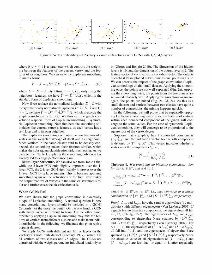
(a) 1-layer (b) 2-layer (c) 3-layer (d) 4-layer (e) 5-layer

Figure 2: Vertex embeddings of Zachary’s karate club network with GCNs with 1,2,3,4,5 layers.

where 0 < γ ≤ 1 is a parameter which controls the weight-ing between the features of the current vertex and the fea-tures of its neighbors. We can write the Laplacian smoothingin matrix form:

Y = X − γD−1LX = (I − γD−1L)X, (10)

where L = D − A. By letting γ = 1, i.e., only using theneighbors’ features, we have Y = D−1AX , which is thestandard form of Laplacian smoothing.

Now if we replace the normalized Laplacian D−1L withthe symmetrically normalized Laplacian D−

12 LD−

12 and let

γ = 1, we have Y = D−1/2AD−1/2X , which is exactly thegraph convolution in Eq. (8). We thus call the graph con-volution a special form of Laplacian smoothing – symmet-ric Laplacian smoothing. Note that here the smoothing stillincludes the current vertex’s features, as each vertex has aself-loop and is its own neighbor.

The Laplacian smoothing computes the new features of avertex as the weighted average of itself and its neighbors’.Since vertices in the same cluster tend to be densely con-nected, the smoothing makes their features similar, whichmakes the subsequent classification task much easier. As wecan see from Table 1, applying the smoothing only once hasalready led to a huge performance gain.

Multi-layer Structure. We can also see from Table 1 thatwhile the 2-layer FCN only slightly improves over the 1-layer FCN, the 2-layer GCN significantly improves over the1-layer GCN by a large margin. This is because applyingsmoothing again on the activations of the first layer makesthe output features of vertices in the same cluster more sim-ilar and further eases the classification task.

When GCNs FailWe have shown that the graph convolution is essentiallya type of Laplacian smoothing. A natural question is howmany convolutional layers should be included in a GCN?Certainly not the more the better. On the one hand, a GCNwith many layers is difficult to train. On the other hand,repeatedly applying Laplacian smoothing may mix the fea-tures of vertices from different clusters and make them indis-tinguishable. In the following, we illustrate this point with apopular dataset.

We apply GCNs with different number of layers on theZachary’s karate club dataset (Zachary 1977), which has34 vertices of two classes and 78 edges. The GCNs areuntrained with the weight parameters initialized randomly as

in (Glorot and Bengio 2010). The dimension of the hiddenlayers is 16, and the dimension of the output layer is 2. Thefeature vector of each vertex is a one-hot vector. The outputsof each GCN are plotted as two-dimensional points in Fig. 2.We can observe the impact of the graph convolution (Lapla-cian smoothing) on this small dataset. Applying the smooth-ing once, the points are not well-separated (Fig. 2a). Apply-ing the smoothing twice, the points from the two classes areseparated relatively well. Applying the smoothing again andagain, the points are mixed (Fig. 2c, 2d, 2e). As this is asmall dataset and vertices between two classes have quite anumber of connections, the mixing happens quickly.

In the following, we will prove that by repeatedly apply-ing Laplacian smoothing many times, the features of verticeswithin each connected component of the graph will con-verge to the same values. For the case of symmetric Lapla-cian smoothing, they will converge to be proportional to thesquare root of the vertex degree.

Suppose that a graph G has k connected components{Ci}ki=1, and the indication vector for the i-th componentis denoted by 1(i) ∈ Rn. This vector indicates whether avertex is in the component Ci, i.e.,

1(i)j =

{1, vj ∈ Ci0, vj 6∈ Ci (11)

Theorem 1. If a graph has no bipartite components, thenfor any w ∈ Rn, and α ∈ (0, 1],

limm→+∞

(I − αLrw)mw = [1(1),1(2), . . . ,1(k)]θ1,

limm→+∞

(I − αLsym)mw = D−

12 [1(1),1(2), . . . ,1(k)]θ2,

where θ1 ∈ Rk, θ2 ∈ Rk, i.e., they converge to a linearcombination of {1(i)}ki=1 and {D− 1

21(i)}ki=1 respectively.

Proof. Lrw and Lsym have the same n eigenvalues (by mul-tiplicity) with different eigenvectors (Von Luxburg 2007). Ifa graph has no bipartite components, the eigenvalues all fallin [0,2) (Chung 1997). The eigenspaces of Lrw and Lsymcorresponding to eigenvalue 0 are spanned by {1(i)}ki=1

and {D− 121(i)}ki=1 respectively (Von Luxburg 2007). For

α ∈ (0, 1], the eigenvalues of (I −αLrw) and (I −αLsym)all fall into (-1,1], and the eigenspaces of eigenvalue 1 arespanned by {1(i)}ki=1 and {D− 1

21(i)}ki=1 respectively. Sincethe absolute value of all eigenvalues of (I − αLrw) and(I − αLsym) are less than or equal to 1, after repeatedly

multiplying them from the left, the result will converge to thelinear combination of eigenvectors of eigenvalue 1, i.e. thelinear combination of {1(i)}ki=1 and {D− 1

21(i)}ki=1 respec-tively.

Note that since an extra self-loop is added to each ver-tex, there is no bipartite component in the graph. Based onthe above theorem, over-smoothing will make the featuresindistinguishable and hurt the classification accuracy.

The above analysis raises potential concerns about stack-ing many convolutional layers in a GCN. Besides, a deepGCN is much more difficult to train. In fact, the GCN usedin (Kipf and Welling 2017) is a 2-layer GCN. However, sincethe graph convolution is a localized filter – a linear combina-tion of the feature vectors of adjacent neighbors, a shallowGCN cannot sufficiently propagate the label information tothe entire graph with only a few labels. As shown in Fig. 1,the performance of GCNs (with or without validation) dropsquickly as the training size shrinks. In fact, the accuracy ofGCNs decreases much faster than the accuracy of label prop-agation. Since label propagation only uses the graph infor-mation while GCNs utilize both structural and vertex fea-tures, it reflects the inability of the GCN model in exploringthe global graph structure.

Another problem with the GCN model in (Kipf andWelling 2017) is that it requires an additional validation setfor early stopping in training, which is essentially using theprediction accuracy on the validation set for model selection.If we optimize a GCN on the training data without using thevalidation set, it will have a significant drop in performance.As shown in Fig. 1, the performance of the GCN without val-idation drops much sharper than the GCN with validation. In(Kipf and Welling 2017), the authors used an additional setof 500 labeled data for validation, which is much more thanthe total number of training data. This is certainly undesir-able as it defeats the purpose of semi-supervised learning.Furthermore, it makes the comparison of GCNs with othermethods unfair as other methods such as label propagationmay not need the validation data at all.

4 SolutionsWe summarize the advantages and disadvantages of theGCN model as follows. The advantages are: 1) the graphconvolution – Laplacian smoothing helps making the classi-fication problem much easier; 2) the multi-layer neural net-work is a powerful feature extractor. The disadvantages are:1) the graph convolution is a localized filter, which performsunsatisfactorily with few labeled data; 2) the neural networkneeds considerable amount of labeled data for validation andmodel selection.

We want to make best use of the advantages of the GCNmodel while overcoming its limits. This naturally leads to aco-training (Blum and Mitchell 1998) idea.

Co-Train a GCN with a Random Walk ModelWe propose to co-train a GCN with a random walk modelas the latter can explore the global graph structure, whichcomplements the GCN model. In particular, we first use arandom walk model to find the most confident vertices – the

nearest neighbors to the labeled vertices of each class, andthen add them to the label set to train a GCN. Unlike in (Kipfand Welling 2017), we directly optimize the parameters of aGCN on the training set, without requiring additional labeleddata for validation.

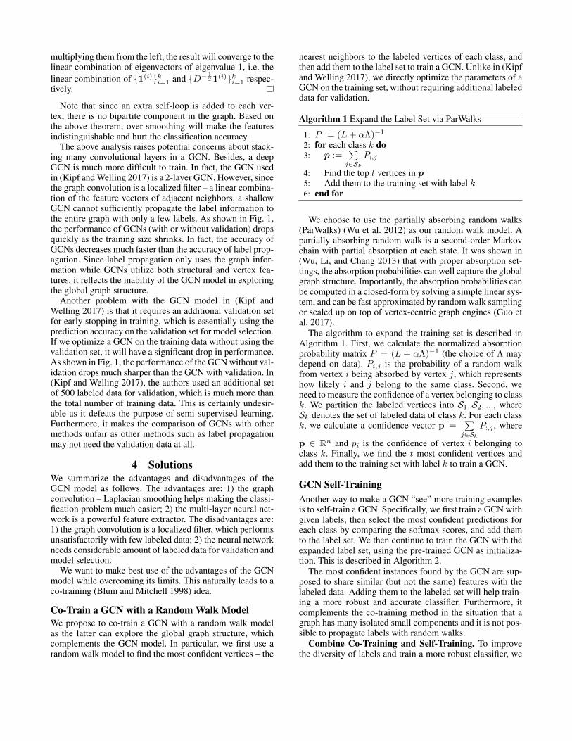
Algorithm 1 Expand the Label Set via ParWalks

1: P := (L+ αΛ)−1

2: for each class k do3: p :=

∑j∈Sk

P:,j

4: Find the top t vertices in p5: Add them to the training set with label k6: end for

We choose to use the partially absorbing random walks(ParWalks) (Wu et al. 2012) as our random walk model. Apartially absorbing random walk is a second-order Markovchain with partial absorption at each state. It was shown in(Wu, Li, and Chang 2013) that with proper absorption set-tings, the absorption probabilities can well capture the globalgraph structure. Importantly, the absorption probabilities canbe computed in a closed-form by solving a simple linear sys-tem, and can be fast approximated by random walk samplingor scaled up on top of vertex-centric graph engines (Guo etal. 2017).

The algorithm to expand the training set is described inAlgorithm 1. First, we calculate the normalized absorptionprobability matrix P = (L + αΛ)−1 (the choice of Λ maydepend on data). Pi,j is the probability of a random walkfrom vertex i being absorbed by vertex j, which representshow likely i and j belong to the same class. Second, weneed to measure the confidence of a vertex belonging to classk. We partition the labeled vertices into S1,S2, ..., whereSk denotes the set of labeled data of class k. For each classk, we calculate a confidence vector p =

∑j∈Sk

P:,j , where

p ∈ Rn and pi is the confidence of vertex i belonging toclass k. Finally, we find the t most confident vertices andadd them to the training set with label k to train a GCN.

GCN Self-TrainingAnother way to make a GCN “see” more training examplesis to self-train a GCN. Specifically, we first train a GCN withgiven labels, then select the most confident predictions foreach class by comparing the softmax scores, and add themto the label set. We then continue to train the GCN with theexpanded label set, using the pre-trained GCN as initializa-tion. This is described in Algorithm 2.

The most confident instances found by the GCN are sup-posed to share similar (but not the same) features with thelabeled data. Adding them to the labeled set will help train-ing a more robust and accurate classifier. Furthermore, itcomplements the co-training method in the situation that agraph has many isolated small components and it is not pos-sible to propagate labels with random walks.

Combine Co-Training and Self-Training. To improvethe diversity of labels and train a more robust classifier, we

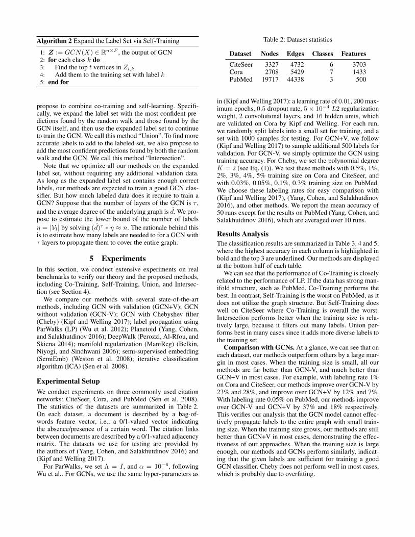
Algorithm 2 Expand the Label Set via Self-Training

1: Z := GCN(X) ∈ Rn×F , the output of GCN2: for each class k do3: Find the top t vertices in Zi,k4: Add them to the training set with label k5: end for

propose to combine co-training and self-learning. Specifi-cally, we expand the label set with the most confident pre-dictions found by the random walk and those found by theGCN itself, and then use the expanded label set to continueto train the GCN. We call this method “Union”. To find moreaccurate labels to add to the labeled set, we also propose toadd the most confident predictions found by both the randomwalk and the GCN. We call this method “Intersection”.

Note that we optimize all our methods on the expandedlabel set, without requiring any additional validation data.As long as the expanded label set contains enough correctlabels, our methods are expected to train a good GCN clas-sifier. But how much labeled data does it require to train aGCN? Suppose that the number of layers of the GCN is τ ,and the average degree of the underlying graph is d. We pro-pose to estimate the lower bound of the number of labelsη = |Vl| by solving (d)τ ∗ η ≈ n. The rationale behind thisis to estimate how many labels are needed to for a GCN withτ layers to propagate them to cover the entire graph.

5 ExperimentsIn this section, we conduct extensive experiments on realbenchmarks to verify our theory and the proposed methods,including Co-Training, Self-Training, Union, and Intersec-tion (see Section 4).

We compare our methods with several state-of-the-artmethods, including GCN with validation (GCN+V); GCNwithout validation (GCN-V); GCN with Chebyshev filter(Cheby) (Kipf and Welling 2017); label propagation usingParWalks (LP) (Wu et al. 2012); Planetoid (Yang, Cohen,and Salakhutdinov 2016); DeepWalk (Perozzi, Al-Rfou, andSkiena 2014); manifold regularization (ManiReg) (Belkin,Niyogi, and Sindhwani 2006); semi-supervised embedding(SemiEmb) (Weston et al. 2008); iterative classificationalgorithm (ICA) (Sen et al. 2008).

Experimental SetupWe conduct experiments on three commonly used citationnetworks: CiteSeer, Cora, and PubMed (Sen et al. 2008).The statistics of the datasets are summarized in Table 2.On each dataset, a document is described by a bag-of-words feature vector, i.e., a 0/1-valued vector indicatingthe absence/presence of a certain word. The citation linksbetween documents are described by a 0/1-valued adjacencymatrix. The datasets we use for testing are provided bythe authors of (Yang, Cohen, and Salakhutdinov 2016) and(Kipf and Welling 2017).

For ParWalks, we set Λ = I , and α = 10−6, followingWu et al.. For GCNs, we use the same hyper-parameters as

Table 2: Dataset statistics

Dataset Nodes Edges Classes FeaturesCiteSeer 3327 4732 6 3703Cora 2708 5429 7 1433PubMed 19717 44338 3 500

in (Kipf and Welling 2017): a learning rate of 0.01, 200 max-imum epochs, 0.5 dropout rate, 5 × 10−4 L2 regularizationweight, 2 convolutional layers, and 16 hidden units, whichare validated on Cora by Kipf and Welling. For each run,we randomly split labels into a small set for training, and aset with 1000 samples for testing. For GCN+V, we follow(Kipf and Welling 2017) to sample additional 500 labels forvalidation. For GCN-V, we simply optimize the GCN usingtraining accuracy. For Cheby, we set the polynomial degreeK = 2 (see Eq. (1)). We test these methods with 0.5%, 1%,2%, 3%, 4%, 5% training size on Cora and CiteSeer, andwith 0.03%, 0.05%, 0.1%, 0.3% training size on PubMed.We choose these labeling rates for easy comparison with(Kipf and Welling 2017), (Yang, Cohen, and Salakhutdinov2016), and other methods. We report the mean accuracy of50 runs except for the results on PubMed (Yang, Cohen, andSalakhutdinov 2016), which are averaged over 10 runs.

Results AnalysisThe classification results are summarized in Table 3, 4 and 5,where the highest accuracy in each column is highlighted inbold and the top 3 are underlined. Our methods are displayedat the bottom half of each table.

We can see that the performance of Co-Training is closelyrelated to the performance of LP. If the data has strong man-ifold structure, such as PubMed, Co-Training performs thebest. In contrast, Self-Training is the worst on PubMed, as itdoes not utilize the graph structure. But Self-Training doeswell on CiteSeer where Co-Training is overall the worst.Intersection performs better when the training size is rela-tively large, because it filters out many labels. Union per-forms best in many cases since it adds more diverse labels tothe training set.

Comparison with GCNs. At a glance, we can see that oneach dataset, our methods outperform others by a large mar-gin in most cases. When the training size is small, all ourmethods are far better than GCN-V, and much better thanGCN+V in most cases. For example, with labeling rate 1%on Cora and CiteSeer, our methods improve over GCN-V by23% and 28%, and improve over GCN+V by 12% and 7%.With labeling rate 0.05% on PubMed, our methods improveover GCN-V and GCN+V by 37% and 18% respectively.This verifies our analysis that the GCN model cannot effec-tively propagate labels to the entire graph with small train-ing size. When the training size grows, our methods are stillbetter than GCN+V in most cases, demonstrating the effec-tiveness of our approaches. When the training size is largeenough, our methods and GCNs perform similarly, indicat-ing that the given labels are sufficient for training a goodGCN classifier. Cheby does not perform well in most cases,which is probably due to overfitting.

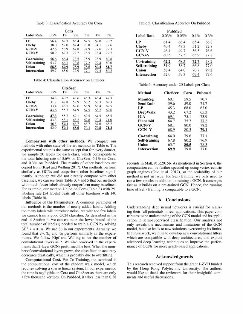
Table 3: Classification Accuracy On Cora

CoraLabel Rate 0.5% 1% 2% 3% 4% 5%

LP 56.4 62.3 65.4 67.5 69.0 70.2Cheby 38.0 52.0 62.4 70.8 74.1 77.6GCN-V 42.6 56.9 67.8 74.9 77.6 79.3GCN+V 50.9 62.3 72.2 76.5 78.4 79.7

Co-training 56.6 66.4 73.5 75.9 78.9 80.8Self-training 53.7 66.1 73.8 77.2 79.4 80.0Union 58.5 69.9 75.9 78.5 80.4 81.7Intersection 49.7 65.0 72.9 77.1 79.4 80.2

Table 4: Classification Accuracy on CiteSeer

CiteSeerLabel Rate 0.5% 1% 2% 3% 4% 5%

LP 34.8 40.2 43.6 45.3 46.4 47.3Cheby 31.7 42.8 59.9 66.2 68.3 69.3GCN-V 33.4 46.5 62.6 66.9 68.4 69.5GCN+V 43.6 55.3 64.9 67.5 68.7 69.6

Co-training 47.3 55.7 62.1 62.5 64.5 65.5Self-training 43.3 58.1 68.2 69.8 70.4 71.0Union 46.3 59.1 66.7 66.7 67.6 68.2Intersection 42.9 59.1 68.6 70.1 70.8 71.2

Comparison with other methods. We compare ourmethods with other state-of-the-art methods in Table 6. Theexperimental setup is the same except that for every dataset,we sample 20 labels for each class, which corresponds tothe total labeling rate of 3.6% on CiteSeer, 5.1% on Cora,and 0.3% on PubMed. The results of other baselines arecopied from (Kipf and Welling 2017). Our methods performsimilarly as GCNs and outperform other baselines signif-icantly. Although we did not directly compare with otherbaselines, we can see from Table 3, 4 and 5 that our methodswith much fewer labels already outperform many baselines.For example, our method Union on Cora (Table 3) with 2%labeling rate (54 labels) beats all other baselines with 140labels (Table 6).

Influence of the Parameters. A common parameter ofour methods is the number of newly added labels. Addingtoo many labels will introduce noise, but with too few labelswe cannot train a good GCN classifier. As described in theend of Section 4, we can estimate the lower bound of thetotal number of labels η needed to train a GCN by solving(d)τ ∗ η ≈ n. We use 3η in our experiments. Actually, wefound that 2η, 3η and 4η perform similarly in the experi-ments. We follow Kipf and Welling to set the number ofconvolutional layers as 2. We also observed in the experi-ments that 2-layer GCNs performed the best. When the num-ber of convolutional layers grows, the classification accuracydecreases drastically, which is probably due to overfitting.

Computational Cost. For Co-Training, the overhead isthe computational cost of the random walk model, whichrequires solving a sparse linear system. In our experiments,the time is negligible on Cora and CiteSeer as there are onlya few thousand vertices. On PubMed, it takes less than 0.38

Table 5: Classification Accuracy On PubMed

PubMedLabel Rate 0.03% 0.05% 0.1% 0.3%

LP 61.4 66.4 65.4 66.8Cheby 40.4 47.3 51.2 72.8GCN-V 46.4 49.7 56.3 76.6GCN+V 60.5 57.5 65.9 77.8

Co-training 62.2 68.3 72.7 78.2Self-training 51.9 58.7 66.8 77.0Union 58.4 64.0 70.7 79.2Intersection 52.0 59.3 69.4 77.6

Table 6: Accuracy under 20 Labels per Class

Method CiteSeer Cora PubmedManiReg 60.1 59.5 70.7SemiEmb 59.6 59.0 71.7LP 45.3 68.0 63.0DeepWalk 43.2 67.2 65.3ICA 69.1 75.1 73.9Planetoid 64.7 75.7 77.2GCN-V 68.1 80.0 78.2GCN+V 68.9 80.3 79.1Co-training 64.0 79.6 77.1Self-training 67.8 80.2 76.9Union 65.7 80.5 78.3Intersection 69.9 79.8 77.0

seconds in MatLab R2015b. As mentioned in Section 4, thecomputation can be further speeded up using vertex-centricgraph engines (Guo et al. 2017), so the scalability of ourmethod is not an issue. For Self-Training, we only need torun a few epochs in addition to training a GCN. It convergesfast as it builds on a pre-trained GCN. Hence, the runningtime of Self-Training is comparable to a GCN.

6 ConclusionsUnderstanding deep neural networks is crucial for realiz-ing their full potentials in real applications. This paper con-tributes to the understanding of the GCN model and its appli-cation in semi-supervised classification. Our analysis notonly reveals the mechanisms and limitations of the GCNmodel, but also leads to new solutions overcoming its limits.In future work, we plan to develop new convolutional filterswhich are compatible with deep architectures, and exploitadvanced deep learning techniques to improve the perfor-mance of GCNs for more graph-based applications.

AcknowledgmentsThis research received support from the grant 1-ZVJJ fundedby the Hong Kong Polytechnic University. The authorswould like to thank the reviewers for their insightful com-ments and useful discussions.

References[Belkin, Niyogi, and Sindhwani] Belkin, M.; Niyogi, P.; andSindhwani, V. 2006. Manifold regularization: A geometricframework for learning from labeled and unlabeled exam-ples. Journal of machine learning research 7:2434.

[Bengio, Delalleau, and Le Roux] Bengio, Y.; Delalleau, O.;and Le Roux, N. 2006. Label propagation and quadraticcriterion. Semi-supervised learning 193–216.

[Blum and Chawla] Blum, A., and Chawla, S. 2001. Learn-ing from labeled and unlabeled data using graph mincuts. InICML, 19–26. ACM.

[Blum and Mitchell] Blum, A., and Mitchell, T. 1998. Com-bining labeled and unlabeled data with co-training. In Pro-ceedings of the 11th annual conference on Computationallearning theory, 92–100. ACM.

[Blum et al.] Blum, A.; Lafferty, J.; Rwebangira, M.; andReddy, R. 2004. Semi-supervised learning using random-ized mincuts. In ICML, 13. ACM.

[Bronstein et al.] Bronstein, M. M.; Bruna, J.; LeCun, Y.;Szlam, A.; and Vandergheynst, P. 2017. Geometric deeplearning: going beyond euclidean data. IEEE Signal Pro-cessing Magazine 34(4):18–42.

[Bruna et al.] Bruna, J.; Zaremba, W.; Szlam, A.; and LeCun,Y. 2014. Spectral networks and locally connected networkson graphs. ICLR.

[Chapelle and Zien] Chapelle, O., and Zien, A. 2005. Semi-supervised classification by low density separation. InProceedings of the Tenth International Workshop on Arti-ficial Intelligence and Statistics, 57–64. Max-Planck-Gesellschaft.

[Chung] Chung, F. R. 1997. Spectral graph theory. Ameri-can Mathematical Soc.

[Defferrard, Bresson, and Vandergheynst] Defferrard, M.;Bresson, X.; and Vandergheynst, P. 2016. Convolutionalneural networks on graphs with fast localized spectralfiltering. In NIPS, 3844–3852. Curran Associates, Inc.

[Glorot and Bengio] Glorot, X., and Bengio, Y. 2010. Under-standing the difficulty of training deep feedforward neuralnetworks. In Proceedings of the Thirteenth InternationalConference on Artificial Intelligence and Statistics, 249–256. PMLR.

[Guo et al.] Guo, H.; Tang, R.; Ye, Y.; Li, Z.; and He, X.2017. A graph-based push service platform. In Interna-tional Conference on Database Systems for Advanced Appli-cations, 636–648. Springer.

[Hammond, Vandergheynst, and Gribonval] Hammond,D. K.; Vandergheynst, P.; and Gribonval, R. 2011.Wavelets on graphs via spectral graph theory. Applied andComputational Harmonic Analysis 30(2):129–150.

[Joachims] Joachims, T. 2003. Transductive learning viaspectral graph partitioning. In ICML, 290–297. ACM.

[Kipf and Welling] Kipf, T. N., and Welling, M. 2017. Semi-supervised classification with graph convolutional networks.In ICLR.

[Lake, Salakhutdinov, and Tenenbaum] Lake, B. M.;Salakhutdinov, R.; and Tenenbaum, J. B. 2015. Human-level concept learning through probabilistic programinduction. Science 350(6266):1332–1338.

[Perozzi, Al-Rfou, and Skiena] Perozzi, B.; Al-Rfou, R.; andSkiena, S. 2014. Deepwalk: Online learning of social repre-sentations. In Proceedings of the 20th ACM SIGKDD inter-national conference on Knowledge discovery and data min-ing, 701–710. ACM.

[Rasmus et al.] Rasmus, A.; Berglund, M.; Honkala, M.;Valpola, H.; and Raiko, T. 2015. Semi-supervised learningwith ladder networks. In NIPS, 3546–3554. Curran Asso-ciates, Inc.

[Rezende et al.] Rezende, D.; Danihelka, I.; Gregor, K.;Wierstra, D.; et al. 2016. One-shot generalization in deepgenerative models. In ICML 2016, 1521–1529. ACM.

[Sandryhaila and Moura] Sandryhaila, A., and Moura, J. M.2013. Discrete signal processing on graphs. IEEE transac-tions on signal processing 61(7):1644–1656.

[Sen et al.] Sen, P.; Namata, G.; Bilgic, M.; Getoor, L.; Gal-ligher, B.; and Eliassi-Rad, T. 2008. Collective classificationin network data. AI magazine 29(3):93.

[Shuman et al.] Shuman, D. I.; Narang, S. K.; Frossard, P.;Ortega, A.; and Vandergheynst, P. 2013. The emerging fieldof signal processing on graphs: Extending high-dimensionaldata analysis to networks and other irregular domains. IEEESignal Processing Magazine 30(3):83–98.

[Talukdar and Crammer] Talukdar, P. P., and Crammer, K.2009. New regularized algorithms for transductive learn-ing. In Joint European Conference on Machine Learningand Knowledge Discovery in Databases, 442–457. Springer.

[Taubin] Taubin, G. 1995. A signal processing approach tofair surface design. In Proceedings of the 22nd annual con-ference on Computer graphics and interactive techniques,351–358. ACM.

[Von Luxburg] Von Luxburg, U. 2007. A tutorial on spectralclustering. Statistics and computing 17(4):395–416.

[Weston et al.] Weston, J.; Ratle, F.; Mobahi, H.; and Col-lobert, R. 2008. Deep learning via semi-supervised embed-ding. In Proceedings of the 25th international conference onMachine learning, 1168–1175. ACM.

[Wu et al.] Wu, X.; Li, Z.; So, A. M.; Wright, J.; and Chang,S.-f. 2012. Learning with Partially Absorbing RandomWalks. In NIPS 25, 3077–3085. Curran Associates, Inc.

[Wu, Li, and Chang] Wu, X.-M.; Li, Z.; and Chang, S. 2013.Analyzing the harmonic structure in graph-based learning.In NIPS.

[Yang, Cohen, and Salakhutdinov] Yang, Z.; Cohen, W. W.;and Salakhutdinov, R. 2016. Revisiting semi-supervisedlearning with graph embeddings. In Proceedings of the33rd International conference on Machine learning, 40–48.ACM.

[Zachary] Zachary, W. W. 1977. An information flow modelfor conflict and fission in small groups. Journal of anthro-pological research 33(4):452–473.

[Zhou et al.] Zhou, D.; Bousquet, O.; Lal, T. N.; Weston, J.;and Scholkopf, B. 2004. Learning with local and globalconsistency. In NIPS 16, 321–328. MIT Press.

[Zhu and Goldberg] Zhu, X., and Goldberg, A. 2009. Intro-duction to semi-supervised learning. Synthesis Lectures onArtificial Intelligence and Machine Learning 3(1):1–130.

[Zhu, Ghahramani, and Lafferty] Zhu, X.; Ghahramani, Z.;and Lafferty, J. D. 2003. Semi-supervised learning usinggaussian fields and harmonic functions. In ICML 2003, 912–919. ACM.