LI, LI, AND PORIKLI: DEEPTRACK 1

DeepTrack: Learning Discriminative FeatureRepresentations by Convolutional NeuralNetworks for Visual Tracking

Hanxi Li12

hanxi.li@nicta.com.au

Yi Li1

http://users.cecs.anu.edu.au/~yili/

Fatih Porikli1

http://www.porikli.com/

1 NICTA and ANU,Canberra, Australia

2 Jiangxi Normal University,Jiangxi, China

Abstract

Defining hand-crafted feature representations needs expert knowledge, requires time-consuming manual adjustments, and besides, it is arguably one of the limiting factors ofobject tracking.

In this paper, we propose a novel solution to automatically relearn the most usefulfeature representations during the tracking process in order to accurately adapt appear-ance changes, pose and scale variations while preventing from drift and tracking failures.We employ a candidate pool of multiple Convolutional Neural Networks (CNNs) as adata-driven model of different instances of the target object. Individually, each CNNmaintains a specific set of kernels that favourably discriminate object patches from theirsurrounding background using all available low-level cues. These kernels are updatedin an online manner at each frame after being trained with just one instance at the ini-tialization of the corresponding CNN. Given a frame, the most promising CNNs in thepool are selected to evaluate the hypothesises for the target object. The hypothesis withthe highest score is assigned as the current detection window and the selected models areretrained using a warm-start back-propagation which optimizes a structural loss function.

In addition to the model-free tracker, we introduce a class-specific version of the pro-posed method that is tailored for tracking of a particular object class such as human faces.Our experiments on a large selection of videos from the recent benchmarks demonstratethat our method outperforms the existing state-of-the-art algorithms and rarely loses thetrack of the target object.

1 IntroductionTracking objects across video frames has long been a fundamental challenge in computervision. In a typical setting, the object location is initialized in the first frame, and the objectwindows in subsequent frames are reported as tracking results.

In general, there are three core tasks to be carried out by an object tracking method: 1)mathematical modelling of the object of interest, 2) searching for the best location of this

c© 2014. The copyright of this document resides with its authors.It may be distributed unchanged freely in print or electronic forms.

2 LI, LI, AND PORIKLI: DEEPTRACK

model in a new frame, and 3) updating the model according to the newly acquired objectlocation. The performance of all these three tasks highly depends on how the underlyingobject region is modelled into a mathematical form, i.e. feature representation. While thereis a plethora of existing methods exploring various combinations of preferred approaches forthese tasks, finding automatically an optimal set of discriminative feature representations toobtain the most robust and accurate tracking performance is still an unsolved problem.

In many early methods, features are manually defined and combined [1, 5, 9, 16]. Eventhough these methods report satisfactory results on individual datasets, hand-crafted se-lection of feature representations would limit the performance of visual tracking. For in-stance, color histogram feature, which would be discriminative when the lighting conditionis favourable, might become ineffective when the object moves under shadow. It is prefer-able to learn a representation, e.g. a filter applied to a low-level cue, from the current datarather than predefining a generic filter for all possible scenarios.

Recently, deep neural networks have gained attention as an alternative solution for var-ious computer vision tasks. Here, deep indicates a multi-layer neural network architecturethat can efficiently capture sophisticated hierarchies describing the raw data. Making thenetwork deeper will raise the learning capacity significantly [3]. In particular, the Convolu-tional Neural Network (CNN) has shown superior performance on standard object recogni-tion benchmarks [13], [14], [4]. With a deep structure, CNN can effectively learn compli-cated mappings while utilizing minimal domain knowledge.

Using offline trained CNN for tracking has been proposed in the past [8], [18]. In [18],the CNN learns filters from a large dataset of natural images. However, this method uses anoff-line trained single CNN and embeds it into an off-the-shelf tracking framework, treatingCNN as a predefined feature extractor.

Immediate adoption of an online CNN idea for visual tracking, however, is not straight-forward. First of all, CNN requires a large number of training samples, which unfortunatelymay not be available in visual tracking as there exist only a few number of positive instancesof the target object particularly at the beginning of the video. Secondly, CNN tends to eas-ily overfit to the most recent observation, e.g. most recent instance kidnapping the model,which may result in drift problem. Besides, CNN training is computationally very intensivefor online visual tracking.

Here, we propose a novel solution to automatically relearn the most useful feature rep-resentations by taking advantage of the deep neural networks while addressing the aboveissues. Our motivation is that by employing a candidate pool of multiple CNNs we cancapture and adapt to the underlying changes in object appearance and pose without over-fitting to the data. While it is plausible to use a single CNN as the object model, traininga pool of separate appearance models for individual instances provides much more flexibleand computationally advantageous representation. We consider object tracking as a consec-utive object-background labelling process. In this spirit, we use CNN to learn discriminativerepresentations that discriminate object and background regions.

Typically, tracking-by-detection approaches rely on predefined heuristics to sample fromthe estimated object location and construct a set of positive or negative samples. Often thesesamples have binary labels, which causes model deterioration in case of a slight inaccuracyduring tracking [9]. To overcome this, our method employs a structural loss function, whichallows us to use a large number of training samples that have different significance levels, toachieve robustness of the model while preventing from the model deterioration. Individually,each CNN maintains a specific set of kernels that favourably discriminate object patchesfrom their surrounding background using all available low-level cues. These kernels are

LI, LI, AND PORIKLI: DEEPTRACK 3

Cue-1

Cue-2

Cue-3

Cue-4

Training patches

Normalized patches

Learned filters in Layer-1

Training faces

Pre-learn

Class-Specific Cue Layer-1

9, 20 × 20 Input Patch

32 × 32 Layer-2

9, 10 × 10 Layer-3

18, 2 × 2

Feature Vector 18 × 1

Output Label

Label 2 × 1

Convolution 13 × 13

Subsampling 2 × 2

Convolution 9 × 9

Subsampling 2 × 2

Fully Connected

Input-Image

32 × 32 Input-Image

32 × 32 Feature Maps

20 × 20 Feature Maps

20 × 20 Feature Maps

20 × 20 Input-Image

32 × 32 Input-Image

32 × 32 Input-Image

32 × 32

Image 32× 32

32× 32

e Maps 20 ×20

e Maps 20 ×20 32× 32 32× 32

32× 32

Class-Specific

Cue

Current frame

Input-Image

32 × 32 Input-Image

32 × 32 Feature Maps

20 × 20 Feature Maps

20 × 20 Feature Maps

20 × 20 Input-Image

32 × 32 Input-Image

32 × 32 Input-Image

32 × 32

Image 32× 32

32× 32

e Maps 20 ×20

e Maps 20 ×20 32× 32 32× 32

32× 32

Cue-1

Input-Image

32 × 32 Input-Image

32 × 32 Feature Maps

20 × 20 Feature Maps

20 × 20 Feature Maps

20 × 20 Input-Image

32 × 32 Input-Image

32 × 32 Input-Image

32 × 32

Image 32× 32

32× 32

e Maps 20 ×20

e Maps 20 ×20 32× 32 32× 32

32× 32

Cue-4

Figure 1: Overall architecture with (red box) and without (rest) the class-specific version.

updated in an online manner at each frame after being trained by just one instance at theinitialization of the corresponding CNN.

For a given frame, we apply a subset of CNNs from the pool to the patches surroundingthe previous object location. For each patch, we determine the best matching CNNs usingthe k-NN and assign the best score as the score of the patch. And the patch with the highestscore is assigned as the current detection. The selected CNN corresponding to the current de-tection is retrained with a warm-start back-propagation scheme using all the labelled patchesfrom the current frame. This enables us to significantly reduce the computational complexityand not distort the other CNNs in the pool. Since we use different cues, we apply an iterativetraining procedure each cues independently then jointly train their fully-connected layers.This makes the training efficient. Empirically we observed that this two-stage iterative pro-cedure is more accurate than jointly training for all cues.

In addition to be able to track any image region, we introduce a class-specific version ofthe proposed method that is tailored for tracking of a particular object class such as face. Inthis version, the corresponding kernels of the specific object category cue is pretrained andfixed during the tracking.

Our experiments on 16 videos from recent benchmarks demonstrate that our method con-sistently outperforms 9 state-of-the-art algorithms and rarely loses the track of the objects.

2 DeepTrack: CNN Architecture

Effective object tracking requires multiple cues, which may include color, image gradientsand different pixel-wise filter responses. These cues are weakly correlated yet contain com-plementary information. Therefore, it is preferable to consider them simultaneously in ascalable neural network. Below, we present the CNN structure for a single cue. Then, wecouple multiple CNNs and construct our CNN architecture. We then introduce the structural

4 LI, LI, AND PORIKLI: DEEPTRACK

learning concept, which takes both patch similarities and their spatial relations into account.

2.1 CNN for a single cueOur CNN for a single cue consists of two convolutional layers1, corresponding sigmoidfunctions as activation neurons and average pooling operators. The dashed gray block inFig. 1 shows the structure of our single cue network, which can be expressed as (32×32)−(10×10×9)− (1×1×18)− (2) in conventional neural network notation.

The input is 32× 32 image patches, which draws a balance between the representationpower and computational load. The first convolutional layer contains 9 kernels each of size13× 13 (an empirical trade-off between overfitting due to a very large number of kernelsand discrimination power), followed by a pooling operation that reduces the obtained featuremap (filter response) to a lower dimension. The second convolutional layer contains 162kernels with size 9× 9. This leads to a 18 dimensional feature vector in the second layer,after the pooling operation in this layer.

The fully connected layer is a logistic regression operation. It takes the feature vectorθ ∈ R18 and generates the score vector s = [s1,s2]

T ∈ R2, with s1 and s2 correspondingto the positive score and negative score respectively. In order to increase the score marginbetween the positive and negative samples, we calculate the final CNN score of patch n asSn = s1 · exp(s1− s2).

2.2 CNN for multiple cuesIn this work, we use 4 image cues generated from the given gray-scale image, i.e., threelocally normalized images with different parameter configurations and a gradient image.The locally normalized image is usually employed in CNNs as the normalization not onlyalleviates the saturation problem but also makes the CNN robust to illumination changes. Onthe other hand, the gradient images capture the shape information of the object and is a goodcomplementary feature to the normalized gray-scale images. In specific, two parameters rµ

and rσ determine a local contrast normalization process and we use three configurations, i.e.,rµ = 3,rσ = 1, rµ = 3,rσ = 3 and rµ = 5,rσ = 5, respectively. We let CNN to selectthe most informative cues in a data driven fashion.

By concatenating the final responses of these 4 cues, we build a fully connected layer tothe binary output vector (the green dashed block in Fig. 1).

2.3 Structural loss functionLet xn and ln ∈ [0,1]T, [1,0]T denote the cue of the input patch and its ground truth label(background or foreground) respectively, and f (xn;Ω) be the predicted score of xn withnetwork weights Ω, in the conventional setting of CNN learning, the objective function of Nsamples in the batch is

L=1N

N

∑n=1‖ f (xn;Ω)− ln‖2 (1)

when the CNN is trained in the batch-mode. Equation 1 is a commonly used loss functionand performs well in binary classification problems. However, for object localization tasks,usually higher performance can be obtained by ‘structurizing’ the binary classifier. The

1Note that here the “convolutional layer” refers to the convolution process, rather than the layers defined in Fig.1

LI, LI, AND PORIKLI: DEEPTRACK 5

advantage of employing the structural loss is the larger number of available training samples,which is crucial to the CNN training. In the ordinary binary-classification setting, one canonly use the training samples with high importance to avoid class ambiguity. In contrast, thestructural CNN is learned based upon all the sampled patches.

In our CNN framework, we modify the original CNN’s output to f (φ〈Γ,yn〉;Ω) ∈ R,where Γ is the current frame, yn ∈ Ro is the motion hypothesis vector of the target object,which determines the object’s location in Γ and o is the freedom degree2 of the transforma-tion. The operation φ〈Γ,yn〉 suffices to crop the features from Γ using the motion yn.

The associated structural loss is defined as

L=1N

N

∑n=1

[∆(yn,y∗) · ‖ f (φ〈Γ,yn〉;Ω)− ln‖2] , (2)

where y∗ is the (estimated) motion state of the target object in the current frame. To define∆(yn,y∗) we first calculate the overlapping score Θ(yn,y∗) [7] as

Θ(yn,y∗) =area(r(yn)

⋂r(y∗))

area(r(yn)⋃

r(y∗))(3)

where r(y) is the region defined by y,⋂

and⋃

denotes the intersection and union operationsrespectively. Finally we have

∆(yn,y∗) =∣∣∣∣ 21+ exp(−(Θ(yn,y∗)−0.5))

−1∣∣∣∣ ∈ [0,1]. (4)

And the sample label ln is set to [1,0] if Θ(yn,y∗) > 0.5 while [0,1] otherwise. From 4we can see that ∆(yn,y∗) actually measures the importance of the training patch n. Forinstance, patches that are very close to object center and reasonably far from it may playmore significant roles in training the CNN, while the patches in between are less important.

3 Tracking with DeepTrackIt is possible to train jointly the above CNN architecture (shown in Fig. 1) as a whole usingthe patches described in Sec. 2.3. However, to make the tracking robust and computationallyefficient, we train each cue and the fully-connected layer iteratively. We also maintain a poolof CNN models for modelling changes over time.

3.1 Online learning: a coordinate-descent approachWe used Stochastic Gradient Decent (SGD) for learning the parameters Ω. Using multipleimage cues leads to a CNN with higher complexity, which implies a low training speed and ahigh possibility of overfitting. Notice that each image cue may be weakly independent, thuswe train the network iteratively.

In particular, we define the model parameters as Ω = w1cov, · · · ,wK

cov,w1f c, · · · ,wK

f c,where wk

cov denotes the filter parameters in cue-k while wkf c corresponds to the fully-connected

layer. After we complete the training on wkcov, we evaluate the filter responses from all the

2In this paper, we set o = 3, i.e., the object bounding box changes in its xy location and the scale.

6 LI, LI, AND PORIKLI: DEEPTRACK

cues in the fully-connected layer and then jointly update w1f c, · · · ,wK

f c with a small learn-ing rate (see Algorithm 1). This can be regarded as a coordinate-descent variation of SGD. Inpractice, we found this strategy effectively curbs the overfitting while increases the trainingspeed. An empirical comparison between the traditional SGD and the proposed coordinate-descent variation is also reported in 4.3.

Algorithm 1 Iterative SGD-based training1: Inputs: Frame image Γ; CNN model (K cues) f (φ〈Γ, ·〉;Ω = w1

cov, · · · ,wKcov,w1

f c, · · · ,wKf c).

2: Given/Estimated y∗; Sample labels l1, l2, · · · , lN ; Sample motion hypotheses y1,y2, · · · ,yN .3: Learning rates r = r

K ; minimal loss ε; training step budget M K.4: for m← 1, M do

5: Calculate loss L= 1N

N

∑n=1

[∆(yn,y∗) · ‖ f (φ〈Γ,yn〉;Ω)− ln‖2]

6: If L≤ ε , break;7: k = mod(m,K)+1;8: Update wk

cov using SGD with learning rate r;9: Jointly update w1

f c, · · · ,wKf c using Gradient Decent with step length r;

10: end for11: Outputs: New CNN model.

3.2 Temporal adaptation with a CNN poolInstead of learning one complicated and powerful CNN model for all the appearance ob-servations in the past, we chose a relatively small number of filters in the CNN within aframework equipped with a temporal adaptation mechanism. Assuming we buffer the mod-els of the CNN during each update, we build a pool of CNN models F = f1, f2, . . . , fQassociated with a prototype set X = x1, x2, . . . , xQ, where prototype xq is a typical positivesample cue3 when the CNN model fq is learned and Q is the size limit of the pool4.

Given a new frame, we randomly generate 1500 motion hypothesisesY = y1,y2, . . . ,yNof the object around its previous motion state. For each hypothesis yn, we select k nearestCNN models in the pool by measuring the similarities between its cue xn and all the pro-totypes in X 5. Then we perform k nearest CNNs for each yn and the hypothesis with thehighest maximal score is chosen as the detected result, i.e.,

y∗ = argmaxyn∈Y

(maxf j∈Nn

f j(φ〈Γ,yn〉;Ω)

), (5)

where Nn is a subset of Y and contains the k nearest CNNs of yn.After detection, we update the selected model f ∗ = argmax f j∈Ny∗ f j(φ〈Γ,yn〉;Ω) and

increase its rank according to its test error on the current frame. The system will then decidewhether to update f ∗ or add a new CNN into the pool, based on the training error. When thepool size reaches the budget Q, the CNN candidates with the lowest rank is replaced. Thedetails of the temporal adaptation mechanism are illustrated in Figure 2. This temporal adap-tation strategy has two advantages: 1) we can accommodate as many as possible appearance

3In this work we use image gradient as the prototype cue and set k = 5, Q = 50.4The idea of using template pool has already shown its superiority for long term visual tracking, see [15]5In this work the similarity is measured in the space obtained via a PCA mapping

LI, LI, AND PORIKLI: DEEPTRACK 7

#34 #162 #208

CNN-1 CNN-2 CNN-3 CNN-20 CNN-4 … CNN-Pool

Prototypes …

… …

Test Est. Train

① Nearest CNNs via prototype matching

② Perform Nearest CNNs

④ Train from CNN-3

⑥ Update CNN-3

⑥ Add a new CNN

⑤ New CNN?

No

Yes

Time axis

Test Est. Train Test Est. Train

③ Select & rank

Figure 2: Illustration of the temporal adaptation mechanism. In the middle row, the test,estimation and training operations are marked in blue, yellow and green blocks respectively.The numbers 1© to 6© indicates the operation order. The bottom row shows the three-stagesoperations on a frame: test, estimation and training. In the frame images, the green bounding-boxes are the negative samples while the red ones denote the positiv samples.

variations without learning an ensemble of CNNs or a very complicated CNN, which is timeconsuming, 2) the associated ranking mechanism can explicitly refine the model pool anddiscard CNNs with low ranking.

3.3 Class-specific trackingIn certain applications, the target object is from a known class of objects such as human faces.Our method can use this prior information to leverage the performance of tracking by traininga class-specific detector. In the tracking stage, given the particular instance information, oneneeds to combine the class-level detector and the instance-level tracker in a certain way,which usually leads to higher model complexity.

The proposed multiple-cue CNN and the coordinate-descent optimization method nat-urally allow class-specific tracking. We first learn a class-level detector by the CNN. TheCNN detector is then used as a special cue in the DeepTrack. In the tracking stage, allthe parameters in the class-cue is fixed except the ones in the fully-connected layer. Theinformation from the class-level and the instance-level are naturally merged via update thefully-connected layer of the joint model.

4 Experiments

4.1 Data and comparison methodsWe evaluate our method on 16 benchmark video sequences that cover most challengingtracking scenarios such as scale changes, illumination changes, occlusions, cluttered back-grounds and fast motion. The first frames of these sequences are listed in Figure 3. We

8 LI, LI, AND PORIKLI: DEEPTRACK

compare our method with 9 other state-of-the-art trackers including TLD [12], CXT [6],ASLA [11], Struck [9], SCM [20], and the classical tracking algorithms, e.g., Frag [1], CPF[16], IVT [17] and MIL [2].

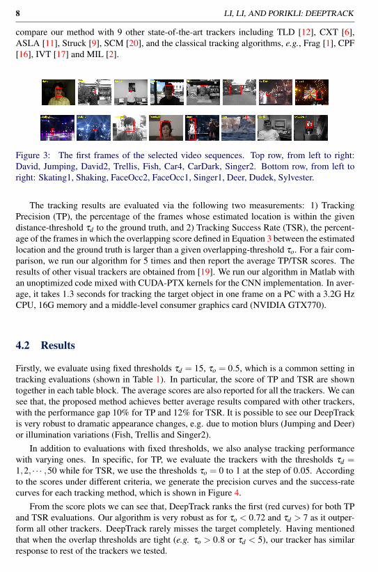
Figure 3: The first frames of the selected video sequences. Top row, from left to right:David, Jumping, David2, Trellis, Fish, Car4, CarDark, Singer2. Bottom row, from left toright: Skating1, Shaking, FaceOcc2, FaceOcc1, Singer1, Deer, Dudek, Sylvester.

The tracking results are evaluated via the following two measurements: 1) TrackingPrecision (TP), the percentage of the frames whose estimated location is within the givendistance-threshold τd to the ground truth, and 2) Tracking Success Rate (TSR), the percent-age of the frames in which the overlapping score defined in Equation 3 between the estimatedlocation and the ground truth is larger than a given overlapping-threshold τo. For a fair com-parison, we run our algorithm for 5 times and then report the average TP/TSR scores. Theresults of other visual trackers are obtained from [19]. We run our algorithm in Matlab withan unoptimized code mixed with CUDA-PTX kernels for the CNN implementation. In aver-age, it takes 1.3 seconds for tracking the target object in one frame on a PC with a 3.2G HzCPU, 16G memory and a middle-level consumer graphics card (NVIDIA GTX770).

4.2 Results

Firstly, we evaluate using fixed thresholds τd = 15, τo = 0.5, which is a common setting intracking evaluations (shown in Table 1). In particular, the score of TP and TSR are showntogether in each table block. The average scores are also reported for all the trackers. We cansee that, the proposed method achieves better average results compared with other trackers,with the performance gap 10% for TP and 12% for TSR. It is possible to see our DeepTrackis very robust to dramatic appearance changes, e.g. due to motion blurs (Jumping and Deer)or illumination variations (Fish, Trellis and Singer2).

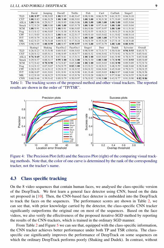
In addition to evaluations with fixed thresholds, we also analyse tracking performancewith varying ones. In specific, for TP, we evaluate the trackers with the thresholds τd =1,2, · · · ,50 while for TSR, we use the thresholds τo = 0 to 1 at the step of 0.05. Accordingto the scores under different criteria, we generate the precision curves and the success-ratecurves for each tracking method, which is shown in Figure 4.

From the score plots we can see that, DeepTrack ranks the first (red curves) for both TPand TSR evaluations. Our algorithm is very robust as for τo < 0.72 and τd > 7 as it outper-form all other trackers. DeepTrack rarely misses the target completely. Having mentionedthat when the overlap thresholds are tight (e.g. τo > 0.8 or τd < 5), our tracker has similarresponse to rest of the trackers we tested.

LI, LI, AND PORIKLI: DEEPTRACK 9

David Jumping David2 Trellis Fish Car4 CarDark Singer2TLD 1.00/0.97 0.98/0.85 1.00/0.95 0.48/0.47 0.98/0.96 0.86/0.79 0.61/0.53 0.04/0.10CXT 1.00/0.83 0.86/0.29 1.00/1.00 0.88/0.81 1.00/1.00 0.30/0.30 0.71/0.69 0.05/0.04ASLA 1.00/0.96 0.29/0.17 1.00/0.95 0.86/0.86 1.00/1.00 1.00/1.00 1.00/1.00 0.03/0.04Struck 0.32/0.24 1.00/0.80 1.00/1.00 0.83/0.78 1.00/1.00 0.97/0.40 1.00/1.00 0.03/0.04SCM 1.00/0.91 0.14/0.12 1.00/0.91 0.86/0.85 0.84/0.86 0.97/0.97 1.00/1.00 0.11/0.16Frag 0.13/0.12 0.96/0.85 0.31/0.30 0.35/0.36 0.52/0.55 0.18/0.21 0.39/0.25 0.16/0.20CPF 0.11/0.03 0.14/0.11 1.00/0.46 0.22/0.17 0.09/0.10 0.03/0.02 0.11/0.02 0.08/0.14IVT 0.95/0.79 0.18/0.10 1.00/0.93 0.32/0.31 1.00/1.00 1.00/1.00 0.77/0.70 0.04/0.04MIL 0.42/0.23 0.76/0.48 0.69/0.32 0.17/0.24 0.34/0.39 0.35/0.28 0.27/0.18 0.18/0.48CNN 0.98/0.95 1.00/0.99 1.00/0.97 0.99/0.97 0.99/1.00 0.97/0.79 1.00/1.00 0.80/0.91

Skating1 Shaking FaceOcc2 FaceOcc1 Singer1 Deer Dudek Sylvester OverallTLD 0.26/0.23 0.33/0.40 0.69/0.83 0.04/0.83 0.98/0.99 0.73/0.73 0.50/0.84 0.94/0.93 0.65/0.71CXT 0.20/0.12 0.05/0.11 0.98/0.95 0.19/0.77 0.80/0.32 0.94/0.92 0.73/0.92 0.76/0.75 0.65/0.61ASLA 0.76/0.69 0.25/0.38 0.67/0.81 0.13/0.31 1.00/1.00 0.03/0.03 0.61/0.90 0.78/0.75 0.65/0.68Struck 0.29/0.37 0.08/0.17 0.99/1.00 0.24/1.00 0.56/0.30 1.00/1.00 0.78/0.98 0.93/0.93 0.69/0.69SCM 0.72/0.42 0.70/0.90 0.74/0.87 0.65/1.00 1.00/1.00 0.03/0.03 0.80/0.98 0.89/0.89 0.72/0.74Frag 0.14/0.12 0.07/0.07 0.54/0.75 0.83/1.00 0.23/0.22 0.18/0.21 0.48/0.59 0.68/0.68 0.38/0.40CPF 0.20/0.19 0.14/0.12 0.29/0.35 0.18/0.52 0.94/0.32 0.04/0.04 0.45/0.69 0.79/0.71 0.30/0.25IVT 0.08/0.07 0.01/0.01 0.91/0.91 0.34/0.98 0.81/0.48 0.03/0.03 0.84/0.97 0.68/0.68 0.56/0.56MIL 0.12/0.10 0.18/0.23 0.55/0.94 0.15/0.76 0.33/0.28 0.08/0.13 0.57/0.86 0.54/0.55 0.36/0.40CNN 0.60/0.46 0.39/0.42 0.89/0.79 0.50/0.97 0.76/0.92 0.98/1.00 0.43/0.77 0.91/0.90 0.82/0.86

Table 1: The tracking scores of the proposed method and other visual trackers. The reportedresults are shown in the order of “TP/TSR”.

0 10 20 30 40 500

0.2

0.4

0.6

0.8

1

Location error threshold

Pre

cis

ion

Precision plots

CNN

SCM

Struck

CXT

ASLA

TLD

IVT

MIL

Frag

CPF

0 0.2 0.4 0.6 0.8 10

0.2

0.4

0.6

0.8

1

Overlap threshold

Success r

ate

Success plots

CNN

SCM

TLD

Struck

ASLA

CXT

IVT

Frag

MIL

CPF

Figure 4: The Precision Plot (left) and the Success Plot (right) of the comparing visual track-ing methods. Note that, the color of one curve is determined by the rank of the correspondingtracker, not the tracker’s name.

4.3 Class specific tracking

On the 8 video sequences that contain human faces, we analysed the class-specific versionof the DeepTrack. We first learn a general face detector using CNN, based on the dataset proposed in [10]. Then, the CNN-based face detector is embedded into the DeepTrackto track the faces on the sequences. The performance scores are shown in Table 2, wecan see that, with prior knowledge carried by the detector, the class-specific CNN trackersignificantly outperforms the original one on most of the sequences. Based on the facevideos, we also verify the effectiveness of the proposed iterative-SGD method by reportingthe results of the CNN-trackers, which is trained in the ordinary SGD manner.

From Table 2 and Figure 5 we can see that, equipped with the class-specific information,the CNN tracker achieves better performance under both TP and TSR criteria. The class-specific cue significantly improves the performance of DeepTrack on some sequences onwhich the ordinary DeepTrack performs poorly (Shaking and Dudek). In contrast, without

10 LI, LI, AND PORIKLI: DEEPTRACK

David Jumping David2 Trellis Shaking FaceOcc2 FaceOcc1 Dudek OverallCNN 0.98/0.95 1.00/0.99 1.00/0.97 0.99/0.97 0.39/0.42 0.89/0.79 0.50/0.97 0.43/0.77 0.77/0.84Class-CNN 1.00/0.98 0.99/0.78 1.00/0.73 1.00/1.00 0.60/0.65 0.84/0.92 0.56/0.94 0.73/0.95 0.84/0.87Normal-SGD 0.52/0.50 0.76/0.68 0.97/0.72 0.65/0.62 0.04/0.05 0.80/0.81 0.20/0.95 0.30/0.68 0.53/0.63

Table 2: The comparison between the DeepTrack and the class-specific DeepTrack. Thereported results are shown in the order of “TP/TSR”. For each video sequence, the bestresult is shown in bold font.

0 10 20 30 40 500

0.2

0.4

0.6

0.8

1

Location error threshold

Pre

cis

ion

Precision plots

Class−CNN

CNN

Normal−SGD

0 0.2 0.4 0.6 0.8 10

0.2

0.4

0.6

0.8

1

Overlap threshold

Success r

ate

Success plots

Class−CNN

CNN

Normal−SGD

Figure 5: The Precision Plot (left) and the Success Plot (right) of the comparing visualtracking methods.

the proposed iterative SGD method, the average performance of the CNN tracker drops byaround 20%.

5 Conclusion

We introduced DeepTrack, a CNN based online object tracker. We employed a CNN ar-chitecture and a structural loss function that handles multiple input cues and class-specifictracking. We also proposed an iterative procedure, which speeds up the training processsignificantly. Together with the CNN pool, our experiments demonstrate that DeepTrackperforms very well on 16 sequences.

References[1] Amit Adam, Ehud Rivlin, and Ilan Shimshoni. Robust fragments-based tracking using

the integral histogram. In CVPR 2006, volume 1.

[2] Boris Babenko, Ming-Hsuan Yang, and Serge Belongie. Visual tracking with onlinemultiple instance learning. Transactions on Pattern Analysis and Machine Intelligence,August 2011.

[3] Y. Bengio, A. Courville, and P. Vincent. Representation learning: A review and newperspectives. Pattern Analysis and Machine Intelligence, IEEE Transactions on, 35(8):1798–1828, 2013.

LI, LI, AND PORIKLI: DEEPTRACK 11

[4] Dan Claudiu Ciresan, Ueli Meier, and Jürgen Schmidhuber. Multi-column deep neuralnetworks for image classification. In CVPR 2012.

[5] Robert T. Collins, Yanxi Liu, and Marius Leordeanu. Online selection of discriminativetracking features. IEEE Transactions on Pattern Analysis and Machine Intelligence, 27(10):1631–1643, 2005. ISSN 0162-8828.

[6] Thang Ba Dinh, Nam Vo, and Gérard Medioni. Context tracker: Exploring support-ers and distracters in unconstrained environments. In CVPR 2011, pages 1177–1184.IEEE.

[7] Mark Everingham, Luc Van Gool, Christopher KI Williams, John Winn, and AndrewZisserman. The pascal visual object classes (voc) challenge. Intl J. of Comp. Vis., 88(2):303–338, 2010.

[8] Jialue Fan, Wei Xu, Ying Wu, and Yihong Gong. Human tracking using convolutionalneural networks. Trans. Neur. Netw., 21(10):1610–1623, October 2010. ISSN 1045-9227.

[9] Sam Hare, Amir Saffari, and Philip HS Torr. Struck: Structured output tracking withkernels. In ICCV 2011, pages 263–270. IEEE.

[10] Vidit Jain and Erik Learned-Miller. Fddb: A benchmark for face detection in uncon-strained settings. Technical Report UM-CS-2010-009, University of Massachusetts,Amherst, 2010.

[11] Xu Jia, Huchuan Lu, and Ming-Hsuan Yang. Visual tracking via adaptive structurallocal sparse appearance model. In CVPR 2012, pages 1822–1829. IEEE.

[12] Zdenek Kalal, Jiri Matas, and Krystian Mikolajczyk. Pn learning: Bootstrapping binaryclassifiers by structural constraints. In CVPR 2010, pages 49–56. IEEE.

[13] Koray Kavukcuoglu, Pierre Sermanet, Y-Lan Boureau, Karol Gregor, Michaël Mathieu,and Yann LeCun. Learning convolutional feature hierachies for visual recognition. InNIPS 2010.

[14] Alex Krizhevsky, Ilya Sutskever, and Geoffrey Hinton. Imagenet classification withdeep convolutional neural networks. In NIPS 2012.

[15] Karel Lebeda, Simon Hadfield, Jiri Matas, and Richard Bowden. Long-term trackingthrough failure cases. In Computer Vision Workshops (ICCVW), 2013 IEEE Interna-tional Conference on, pages 153–160. IEEE, 2013.

[16] Patrick Pérez, Carine Hue, Jaco Vermaak, and Michel Gangnet. Color-based proba-bilistic tracking. In ECCV 2002.

[17] David A. Ross, Jongwoo Lim, Ruei-Sung Lin, and Ming-Hsuan Yang. Incrementallearning for robust visual tracking. Intl. J. Comp. Vis, 77(1-3):125–141, May 2008.ISSN 0920-5691.

[18] Naiyan Wang and Dit-Yan Yeung. Learning a deep compact image representation forvisual tracking. In NIPS 2013.

12 LI, LI, AND PORIKLI: DEEPTRACK

[19] Yi Wu, Jongwoo Lim, and Ming-Hsuan Yang. Online object tracking: A benchmark.CVPR 2013.

[20] Wei Zhong, Huchuan Lu, and Ming-Hsuan Yang. Robust object tracking via sparsity-based collaborative model. In CVPR 2012, pages 1838–1845. IEEE.