UNCLASSIFIED

Defense Technical Information CenterCompilation Part Notice

ADP014041TITLE: Doppler Properties of Airborne Clutter

DISTRIBUTION: Approved for public release, distribution unlimitedAvailability: Hard copy only.

This paper is part of the following report:

TITLE: Military Application of Space-Time Adaptive Processing [Lesapplications militaires du traitement adaptatif espace-temps]

To order the complete compilation report, use: ADA415645

The component part is provided here to allow users access to individually authored sectionsf proceedings, annals, symposia, etc. However, the component should be considered within

-he context of the overall compilation report and not as a stand-alone technical report.

The following component part numbers comprise the compilation report:ADP014040 thru ADP014047

UNCLASSIFIED

2-I

Doppler Properties of Airborne Clutter

Richard KlemmFGAN-FHR, Neuenahrer Str. 20, D 53343 Wachtberg, Germany

Tel +49 228 9435 377; Fax +49 228 9435 618; email r.klemm@fgan.de

AbstractDetection of slowly moving targets by air- and spaceborne MTI radar is heavily degraded by the motion inducedDoppler spread of clutter returns. Space-time adaptive processing (STAP) can achieve optimum clutter rejectionvia implicit platform motion compensation. In this report the fundamentals and properties of STAP applied toair- and spaceborne MTI radar are summarised. The effect of platform motion on the characteristics of airborneclutter is discussed. The performance of the optimum space-time processor is shown. Comparison with spatialor temporal only techniques illustrate the importance of space-time processing.

1 Introduction

The main application of space-time adaptive processing (STAP) is the suppression of clutter received by amoving radar. In this case we talk about space-slow time (pulse-to-pulse) processing. The radar: platformmotion causes clutter returns to be Doppler shifted. The Doppler shift is proportional to the platform velocityand the angle of arrival. The total of all clutter arrivals sums up in a Doppler broadband clutter echo. Targetswhose Doppler frequencies fall into the clutter Doppler bandwidth may be difficult to detect. It should benoted that most moving targets are "slow" or low Doppler targets, either because they are slow or exhibit a lowDoppler due to their motion direction. For a radar on a satellite (10 km/s) all targets near the ground (jet aircraft300 m/s) are slow targets.

Other important techniques operate in the space-fast time (range equivalent) domain. They are used toeither suppress jammers in broadband array radar or for mitigating terrain scattered jamming.

Space-time processing needs space-time data to operate on. Space-time data are obtained from a radarwhich has a phased array antenna with multiple outputs (spatial dimension), and transmits coherent pulse trains(temporal dimension).

1.1 The principle of adaptive clutter suppression

1.1.1 Practical application: adaptive clutter filter for surveillance radar

The following experiment conducted in the early 1970's (BUHRING & KLEMM [6]) is decribed briefly to il-lustrate the principle of adaptive clutter filtering. This filter was designed to suppress weather clutter withunknown centre Doppler frequency and bandwidth. This adaptive MT1 systems was operated with a conven-tional groundbased surveillancde--radar with rotating reflector antenna. Figure 1 shows the block diagram of-an adaptive FIR filter based on the prediction error filter principle. The filter coefficients were estimated inreal-time and the echo data were clutter filtered during the following revolution of the antenna.

In Figure 2 the filtering effect is demonstrated using simulated clutter. The picture shows a photograph of aPPI (pla position indicator) screen. The zero Doppler filter has been switched off so that a lot of ground cluttercan be noticed. The spokes are the simulated clutter (for simplicity this clutter was simulated independentof range). The available radar operated in L-band which is quite insensitive to weather. Therefore, to havereproduceable clutter conditions a hardwired simulator was developed. The clutter filter was adapted based onclutter data in the window on the right. As can be seen the clutter has been removed and a (true) target is visible.

Figure 3 and 4 show suppression of a real weather cloud before and after filtering. Except for a few falsealarms the weather clutter has been removed. The air targets (big spots on the left) did not do us the favour toenter our measurement window, they just bypass it1 .

'No responsible pilot will enter a thunder storm deliberately.

Paper presented at the RTO SET Lecture Series on "Militay Application of Space-Time Adaptive Processing",held in Istanbul, Turkey, 16-17 September 2002; Wachtberg, Germany. 19-20 September 2002;

Moscow, Russia, 23-24 September 2002, and published in RTO-EN-02 7.

2-2

1.2 The History of STAP

In the following two sections a brief review of the history of research and experimental work on STAP is given.

1.2.1 Theoretical work (Table 1)

Table I includes a number of publications which represent milestones in the evolution of STAR This selectionof papers is certainly not exhaustive but to our opinion representative. In some cases merely the earliest papersrather than the most significant papers are quoted. 'In the meantime special journal issues (# 20,21) and tutorials(# 12,19,20) on STAP are available.

The original idea of reducing the clutter spectrum via motion compensation originates from ANDERSON (#

1). This paper was written before digital technotogy was available. The DPCA technique SKOLNIK (# 2) wasalso originally invented for use with for implementation in microwave technology. This technique compensatesphysically or electronically for the platform motion in a non-adaptive fashion. The paper by BRENNAN &REED (# 3) is the basis for all future space-time processing. It deals with interference rejection in broadbandarrays. This principle was analysed in some detail by COMPTON (# 7). The first paper on STAP was writtenby BRENNAN et al. (# 4). Here the optimum (maximum likelihood) processor applied to clutter rejection formoving radar has been described and analysed. Starting from (# 4) KLEMM discovered that the size of theclutter subspace is about N + M under certain conditions which gave rise to manyfold research on subspaceprocessor architectures (# 8, 9, 12, 13, 18, 20). Later on an extension of this result became known as "Brennan'sRule" (# 10). Problems of real-time implementation of STAP processors have been discussed by FARINA etal. (# 11). WARD (# 15) presented angle and Doppler estimation errors for STAP radar. ENDER (# 17)demonstrated the detection and re-positioning of moving targets in SAR images obtained with the multi-channelSAR AER II. DOHERTY et al. and JOUNY et al. (# 16) used STAP techniques to mitigate the effect of terrainscattered jamming. STAP in conjunction with bistatic radar has been discussed by KLEMM (# 23). A recenttrend of moving reconnaissance function from airborne to space-borne platforms can be noticed (COVAULT(# 24)). Besides the STAP research activities in the USA and Europe some considerable interest of Chinesescientists in STAP can be noticed (# 6).

1.212 Experiments and Systems (Table 2)

In Table 2 experimental and operational STAP systems are listed. The first (non-adaptive) DPCA experimentinvolving an array antenna has been carried out by Tsandoulas (# 1). The NRL (# 3) and MCARM experi-ments (# 4) use linear sidelooking arrays. Both programs lead to many detailed investigations on possibilitiesof airborne clutter rejection. A large number of publications originate from these programs, dealing with var-ious research topics such as clutter homogeneity, sidelobe Doppler clutter, knowledge-based MTI processing,subspace techniques-(e.g., E - A), and bistatic operation (# 11). The Mountaintop program (# 5) was started in1990 to study advanced processing techniques and technologies to support the requirements of future airborfieearly warning radar platforms. In particular the effect of terrain scattered jamming has been studied. In Europethe AER I1 program (# 7, Germany), the DO-SAR experiment (# 8, Germany) and the DERA experiment (# 9,UK) have been conducted.

There are three operational systems with space-time ground clutter rejection capability (Joint STARS (U2), AN/APG-76 (# 6), and the AN/APY-6). The first one has a 3-aperture sidelooking array antenna and hasbeen flown in the Gulf War. The AN/APG-76 is a forward looking nose radar and the AN/APY-6 has bothsidelooking and forward looking capability. From the available literature it is not obvious whether these systemare based on adaptive algorithms (STAP) or used some non-adaptive DPCA-like techniques.

1.2.3 Historical note

The non-adaptive DPCA technique has been described already in SKOLNIK ed. [39]. Research on space-timeadaptive processing started with the paper by BRENNAN et al. [4] in 1976 on space-time MTI (moving target

2-3

indication) processing for airborne radar. Very little has been published in the following years. In 1983 theauthor introduced the concept of eigenanalysis of the space-time clutter covariance matrix which opened thehorizon towards subspace techniques for real-time applications [21 ]. A number of follow-up papers by theauthor have been concerned with various suboptimum approaches based on order reducing transforms of thesignal subspace. These papers have been summarized in a book on STAP (KLEMM [26]). Since 1990 researchactivities on STAP increased tremendously, particularly in the USA (e.g. WARD [46], WANG & CA] [43]), inChina (e.g. WANG & BAO [44]), in the UK (RICHARDSON & HAYWARD [35]), and in Italy FARINA et al.[15]).

2-4

# year subject authors1 1958 First paper on motion compensated MTI Anderson [I]2 1970 DPCA Skolnik [39]3 1973 Theory of adaptive radar Brennan & Reed [3]4 1976 First paper on STAP Brennan et al. [4]5 1983 Dimension of clutter subspace Klemm [21]6 P 1987 First Chinese papers e.g. Wang & Bao [44]7 1988 Broadband jammer cancellation Compton [9, 8]8 1990 Space-time FIR filter Klcmm & Endcr [22]9 1992 Spatial transform techniques Klemm [23]

10 1992 Brennan's Rule Brennan & Staudaher [5]11 1992 Real-time implementation of STAP Farina et al. [15]12 1994 Report on STAP Ward [46]13 1994 Beam/Doppler space processing Wang & Cai [43]14 1995 STAP for forward looking arrays Richardson & Hayward [35]

Klemm [24]15 1995 Angle/velocity estimation with STAP radar Ward [47]16 1995 Mitigation of terrain scattered jamming Doherty [11 ], Jouny et al. [20]17 1996 STAP for SAR Ender [13]18 1996 r, - A STAP Wang etal. [45]19 1996 Effect of platform maneuvers Richardson et al. [36]20 1998 lEE Colloquium on STAP Klemm (chair) [25]21 1998 Textbook on STAP Klemm [26]22 1998 Effect of range walk Kreyenkamp [33]23 1999 lEE ECEJ special issue on STAP Klemm (ed) [28]24 1999 IEEE Trans. AES: Special issue on STAP Melvin (ed.)[32]

and Adaptive Arrays25 1999 STAP with bistatic radar Klemm [27]26 1999 STAP for future observation satellites Covault [10]

Table 1. Some milestones in STAP research

2-5

rne•lestimation of the I-Iinversion of theH

processed temporal clutter -- o temporal clutter select 1. rowproceiaseeecho data covarance matrix covariance matrix

Doppler Ifiltering filter dtcibank detection

b& display

T range

processedecho data

Figure 1: Block diagram of adaptive temporal clutter filter

# year system authors1 1973 DPCA with array antenna (flight experiment) Tsandoulas [42]2 1991 Joint STARS antenna Shnitkin [38]3 1992 NRL experiment Lee & Staudaher [34]4 1994 MCARM experiment Babu [2]5 1994 Mountaintop Titi [41]6 1996 AN/APG-76 sidelooking airborne array radar Tobin [40]7 1996 AERII Ender [12]8 1996 Dornier's DO-SAR Hippler & Fritsch [19]9 1996 DERA STAP experiment Coe et al. [7]

10 1998 AN/APY-6 airborne array radar Gross & Holt [ 16]11 1999 STAP with bistatic radar Sanyal et al. [37]

Table 2. Existing STAP systems

2-6

Figure 2: Adaptive suppression of simulated weather clutter

Figure 3: Weather clutter before adaption

2-7

Fu

Figure 4: Weather clutter after a'daption

2-8

2 Principle of air- and spaceborne MTI radar

In this section some important features of airborne clutter echoes are briefly discussed. The efficiency of space-time clutter suppression depends significantly on these properties. For definition of the geometry see Figure 5.It shows two important cases (sidelooking and forward looking arrays).

2.1 Effect of Platform Velocity

2.1.1 Models of clutter and target

The results presented in this paper have been calculated on the basis of simple models for target and interference.For the sake of brevity we give here only the models as used in the evaluation. For more details the reader isreferred to [26, chapter 2].

Clutter

The NM x NM clutter covariance matrix has the form

t Q11 Q12 ... Q1MQ= Q21 QVz ... Q2M I - (1)

QMI QM .. Q M*I

where the indices of the submatrices m,p denote time (pulse repetition intervals) while the indices i, k runinside the submatrices and denote space (sensors). N is the number of sensors and AT the number of coherentlyprocessed echoes. The elements of Q are integrals over a full range circle

(C) 27q =n Ci]_ PrnpPi-k (2)

x D 2 (0)/L,2 (ýo) G (Vo, 77t) G* (Vo, p)

4,(0m.P(•p, vp)40k (cp)dp + PN

M,p= 1...M i,k= I...N

where P, is the clutter power at the single element at a certain instant of time and 1.r the receiver noise power.The other symbols denote as follows: Vo azimuth, s. Figure 5; A complex clutter amplitude; D(Wo) sensordirectivity pattern; L(o) clutter reflectivity; Pk spatial (sensor-to-sensor) correlation which is not consideredhere; Pmp temporal (echo-to-echo) correlation; G(ýo, m) transmit directivity pattern. The temporal and spatialphase terms are as follows

, (Y nm= exp•j"--2vprnTcos o cos O]

= exp[j- (Xi cos W + yi sin ý') (3)

x cos 0 - zi sin 0]

The indices 1, n of the NAM x NM covariance matrix are related to the sensor indices i, k and echo indicesm, p through

I (-(m-1)N+i m=1...M; i =-...N (4)

7= (p - 1)N + k p =1... M; k=1 ... N (5)

2-9

Noise

Receiver noise is assumed to beuncorrelated in space and time

rPn P (6pE{nrnn,,} {= •: m p (6)

n* IP. i = kE~ v .% iJ (7)kJn 0 i 5k k

where Pn denotes the white noise power.

Target

A target at azimuthal position p moving at a radial velocity Vad produces the following space-time signal atthe array output

smi (')= Aexptj 2 (8)

x (2 Vad.m2' + (xi cos Wt + yi sin 'pt) cos 0

-zi sin )]

m= 1...M -i=I...N

2.1.2 The Isodops

Surfaces of constant Doppler are given by cones. Intersections of such cones with the planar ground results ina set of hyperbolas as shown in Figure 6 for horizontal flight and flat earth. The radar platform moves from leftto right. Maximum Doppler is encountered at 00 (positive Doppler) and 180' (negative Doppler), zero Dopplerat 900 2700.

2.1.3 Impact of Array Geometry

Only one quadrant of the isodop field is shown in Figure 7 (thin curves).The axis of a linear array in sidelooking orientation coincides with the flight path. Therefore, curves of

constant look direction are again hyperbolas on the ground (fat curves). The beam traces of a linear sidelookingarray coincide with the isodops. This means that the clutter Doppler is range independent. This importantproperty has implications on clutter rejection.

The axis of a forward looking linear array is perpendicular to the flight axis. Therefore, the set of beamtraces are rotated by 90", s. Figure 8. Now one can notice that beam traces and isodops cross each otherfrequently. For a forward looking array the Doppler frequency of clutter echoes depends- obviously on range.The range dependency occurs especially at short range, that is, where the range is of the order of magnitude ofthe platform height above ground.

2.1.4 Azimuth-Doppler Clutter Trajectories

Figure 9 shows the trajectories of clutter spectra in the azimuth2 (abszissa) - Doppler (ordinate) plane. The fourplots have been calculated for different crab angles 4'. For ?p = V' (sidelooking array) all the clutter power islocated on the diagonal of the plot while for increasing crab angle one obtains ellipses. Finally, ?P = 91Y meansa forward looking array, with the clutter power located on a circular trajectory.

Clutter echoes depend in general on range. First of all the backscattered clutter power decreases with rangeaccording to the radar equation: P, acYs.

2cos (P

2-10

Doppler-range depence

The range dependence of the clutter Doppler frequency has already been addressed in the context of isodops.It follows from the above considerations that the clutter Doppler is constant with range for a sidelooking array.-Therefore, all four curves calculated for different ranges coincide (Figure 9a). From Figure 9d it is obvious thatfor a certain look direction the Doppler frequency increases with range in case of a forward looking array3 .

2.2 Comparison of Spatial, Temporal and Space-Time Processing

The principle of space-time adaptive processing for clutter rejection in moving radars is illustrated in Figure11. A sidelooking sensor configuration was assumed. The clutter spectrum extends along the diagonal of thecos Po-wD plot. Notice the modulation by the transmit beam.

Conventional temporal processing means that the projection of the clutter spectrum onto the wD axis iscancelled via an inverse filter. Such filter is depicted in the back of the plot. As can be seen the clutter notch isdetermined by the projected clutter mainlobe which is a Doppler response of the transmit beam. Slow targetsare attenuated.

Spatial processing as being used for jammer nulling requires that the clutter spectrum is projected onto thecos ýo axis. Applying an inverse spatial clutter filter, however, forms a broad stop band in the look direction sothat the radar becomes blind. Both fast and slow targets fall into the clutter notch.

Space-time processing exploits the fact that the clutter spectrum is basically a narrow ridge. A space-time clutter filter, therefore, has a two-dimensional narrow clutter notch so that even slow targets fall into thepassband.

3 This follows from the depression angle term cos 0 in (3).

2-11

90

100z frad ,nsidelooking forward looking I 6

8

R' /H 6'

9'o

901-

xx

Figure 8: Beam traces (fat) and isodops for fieorwarFigue Figuernet6: The aisrdorns ann, aaray ng array

2-12

0 0 ....

a. , b.,

o 0

C. d.-10 1 1 0 1 inverse temporal clutter filter

Figure 9: fir. - cos ýp clutter trajectories for linear ar- -fitter.

rays: a. ?p = 00; b. ?p = 300; c. 0' = 600; d. 0 900; so

from inside to outside: R/H =1.5; 2; 2.5; 3

0.-clutter notch Doppler-azimuth

0.8-

0.7- Figure 11: Principle of space-time clutter filtering(sidelooking array antenna)

0.6-

0.5-

0.4

0.3-

0.2

0.10 2 4 6 8 10

R/H

Figure 10: Range dependence of the clutter Dopplerfrequency for forward looking array: +,6 = 900 (lookdirection~fiight direction); x [3 = 600; * 63 = 30'

2-13

3 Characteristics of Air- and Spaceborne Clutter

3.1 The Space-time Covariance Matrix

The space-time covariance matrix was defined in eqs. 1, 2. Figs. 12, 13 show the modulus of typical space-timecovariance matrices. As can be seen from Fig. 12 the spatial submatrices are unity matrices with the diagonal

shifted with the temporal indices Mp. In case of pure spatial processing we would deal with a N x N

unity matrix only. In this case no substantial gain in clutter rejection can be achieved. Through spacetimeprocessing we obtain the other correlation ridges in the matrix which provide the correlation required for clutter

cancellation. If we use directive sensors and a directive transmit array some additional correlation comes up ascan be seen in Fig. 13. Fig. 14 shows a space-time covariance matrix for noise jamming. As can be seen thereis no temporal correlation.

3.2 Clutter Spectra

3.2.1 Eigenspectra

The concept of eigenanalysis of space-time clutter covariance matrices was introduced by the author [211. The

eigenspectrum (rank ordered sequence of eigenvalues) shows how large the clutter subspace is.The elements of the space-time covariance matrix are calculated as

q1. = E{cimClp} + P4ikrp (9)

where Cim is the space-time clutter signal. The spatial (sensor) indices i, k and the temporal (echo pulse) indicesm.,p are related with the matrix indices through

1=(rn-1)N-+ i rn=l...M; i=1...N (10)

n=-(p-1)N+k p=1 ... M; k=l...N (11)

PF, is the receiver noise power and &ikmp the Kronecker symbol. It was found in [21 ] that for a sidelooking

equidistant array and the PRF chosen so that DPCA conditions are fulfilled (see section 4.1.1) the number ofeigenvalues is

Ne =N+M- 1.

This figure determines the minimum size of the number of degrees of freedom of the space-time clutter filter.4

3.2.2 Power Spectra

Based on the space-time clutter+noise covariance matrix azimuth-Doppler spectra can be generated, either by2D Fourier transform of the covariance matrix, or by use of one of the well-known high resolution powerestimators.

Let us consider a covariance matrix of the form

R = E{xx*} = S + N (12)

where N is the noise component and S includes all kind of signal or interference. Then the output of a signalmatched filter is simply

YsM(O) =x* s(O) (13)

and the normalised power output is

PSM(o)= s(O)Rs(O) (14)s*(O)s(E)(

4Actually in [21] it reads N,, = N + M. the correct number is N, N + M_ 1.

2-14

s(O) is a steering vector which seeks for signal components s(Oi) in R. P(1) attempts to become maximumwherever the steering vector s(O) coincides with a signal vector s(OQ) in R. For sinusoidal signals the signalmatched filter becomes the 2D Fourier transform.

Fig. 18 shows a 2D Fourier clutter spectrum. One recognises the main beam response and the sidelobe re-sponse along the diagonal. In addition there are spurious Doppler and azimuthal sidelobes which are responsesof the spatial and temporal FT to the main beam clutter. Notice that only the clutter along the diagonal is phys-ical clutter, the sidelobes along the Doppler and azimuth axes are artifacts. Similar relations can be observed ifHamming weighting is applied in space and time (Fig. 19).

The minimum variance estimator has proven to be the most useful because its response is closest to theclutter contained in the covariance matrix. In analogy with (19) the minimum variance estimator becomes

wMV = tR71s (15)

with -y = (s*R- 1 s)-1. The output power is

P~v (0) =(s*(0)R-ls(0))- (16)

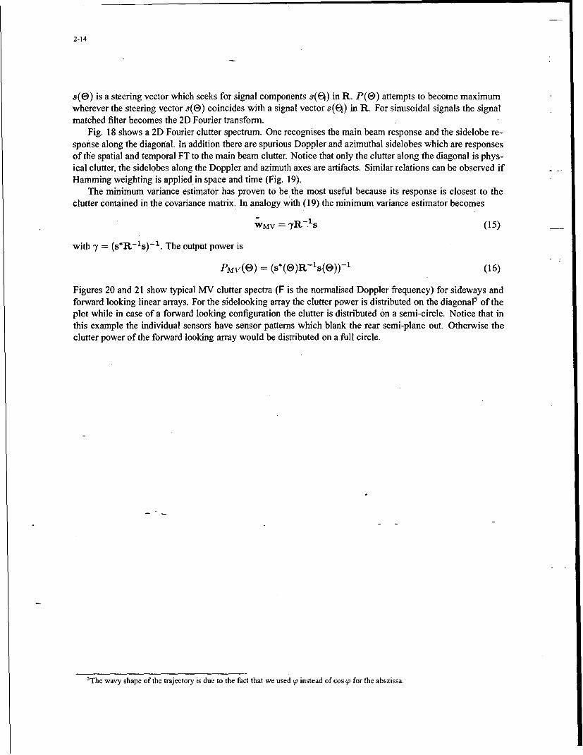
Figures 20 and 21 show typical MV clutter spectra (F is the normalised Doppler frequency) for sideways andforward looking linear arrays. For the sidelooking array the clutter power is distributed on the diagonal5 of theplot while in case of a forward looking configuration the clutter is distributed on a semi-circle. Notice that inthis example the individual sensors have sensor patterns which blank the rear semi-plane out. Otherwise theclutter power of the forward looking array would be distributed on a full circle.

5The wavy shape of the trajectory is due to the fact that we used ýp instead of cos p for the abszissa.

2-15

0120

40, 40,

02

660 00

2 D 0 .3 0 4.. o "-: /•. •o o .20' 3010O 20

0 0 1 " 0 1

Figure 12: Modulus of the clutter covariance matrix Figure 14: Jammer covariance matrix (sidelooking'ar-vs horizontal and vertical index (sidelooking linear ar- ray, N=12. M=5, I jammer, absolute values)ray, N=12, M=5, omnidirectional sensors and trans-mission)

53

400120.0

0 3

o 0 .4060

1-c2020

010

0 0

Figure 15: Eigenspectra of a spatial covariance matrix.

Figure 13: Modulus of the clutter covariance matrix vs N = 72, M = 1; o omnidirectional sensors and trans-horizontal and vertical index (sidelooking linear array, mission; * directive sensors;- x directive sensors andN=12, M=5, directive sensors and transmission) transmission

2-16

so

40

01

30 to.

-20•20 to

-300

10ý -40,

-50

S-03 - • ' 165F 0 • 125

"°o 10 2 0 - 40 -- 6-0 70 00 03 ,• (r0.6 5

Figure 16: Eigenspectra of a space-time covariancematrix (sidelooking array). N = 24, Al = 3; o omni- Figure 18: Fourier clutter spectrum (sidelooking array,

directional sensors and transmission; * directive sen- ýOL 90')sors; x directive sensors and transmission

40 0.

30

-20-

'o 20: 1 -30

-50

10-

7 F 0 "12S. •/

-101 0 30 1 20 30 40 50 00 70 60o o

Figure 17: Eigenspectra of a space-lime covariance Figure 19: Fourier clutter spectrum with spatialmatrix (forward looking array). N = 24, M = 3; o and temporal Hamming weighting (sidelooking array,omnidirectional sensors and transmission; * directive ýL 00)sensors; x directive sensors and transmission

2-17

20,

85

06 5

Figure 20: MV clutter spectrum (sidelooking array,

S0L =450)

101

-20,

-30,

-40

-50O56

F 35

-0.6 -85

Figure 21: MV spectrum for forward looking lineararray

)

2-18

4 The Optimum Space-Time Processor

4.1 Historical: The Displaced Phase Center Antenna (DPCA)

4.1.1 The DPCA technique

DPCA (displaced phase centre antenna) is a technique which compensates physically for the motion of theradar platform to reduce the effect of motion induced Doppler spread of clutter returns. Consider two antennasin sidelooking configuration as shown in Figure 22. At time m = 1 they assume the dashed position, at timem = 2 the solid one. As can be noticed the first antenna at in = 1 assumes the position of the second sensorat time ni = 2. This is equivalent to having one antenna fixed in space 6 for the duration of one pulse interval.Clutter suppression is done by subtracting so that the clutter remainder becomes E = (2 - C21. If c12 = C21

perfect cancellation is obtained. Notice that this technique was implemented in RF technology long time beforethe age of digital signal processing.

4.1.2 A note on DPCA and STAP

For more than 3 decades the DPCA principle (motion compensation by spatial coincidence of sensor positions,s. section 4.1.1 and Figure 22) has been considered the physical background of space-time clutter rejection.More recently, numerical investigations have shown that forward looking arrays (which do not have the DPCAproperty) work as well with space-time adaptive processing.

This reveils that the function of STAP is not based on a DPCA geometry. The space-time filtering is justbased on the fact that airborne clutter echoes are signals depending on the two variables space and time, andthey are bandlimited in the Doppler as well as in the azimuth dimension. If such signals are properly sampledin space (sensor displacement) and time (PRF) any kind of filtering can basically by applied without aliasinglosses. The property of slow target detection is based on the special shapes of such clutter spectra (narrowridge). STAP is not based on DPCA. DPCA is merely a special case of STAP. The DPCA property plays a rolein the context of compensating for the effects of system bandwidth.

4.2 The LR-Test for 2-D Vector Quantities

The principle of detecting a signal vector s before a noisy background given by q is briefly summarized. Letus define the following complex vector quantities:

q2 S2 X2q - s= . ; x= ) (17)

qN SN X-

where qm,sm and Xm are the spatial subvectors (signals at the array output) at the m-th pulse repetition interval.In general the noise vector consists of a correlated part c (e.g. jammer, clutter) and an uncorrelated part n (e.g.receiver noise):

q=c+n (18)

The signal vector s is assumed to be deterministic. x is the actual data vector which may be noise only(x = q) or signal-plus-noise (x = q + s). The problem of extracting s optimally out of the background noiseq is solved by applying the well-known linear weighting

Wopt = YQ-'s (19)

6 Due to the factor of 2 in the Doppler term 2rnvpT the antenna motion during one PRI is only half the antenna spacing. It isimportant that phase coincidence of clutter echoes occurs.

2-19

A block diagram of the optimum processor is shown in Fig. 23. The spatial dimension is given by the N antennaelements while the temporal dimension is given by shift registers where M subsequent echoes are stored. Thesespace-time data are multiplied with the inverse of the space-time adaptive clutter covariance matrix for cluttercancellation. The output signal are -then fed into a space-time weighting network whose coefficients form aspace-time replica (beamformer and Doppler filter) of the desired signal.

4.2.1 Performance of the Optimum Processor

The efficiency of any linear processor w can be characterized by the improvement factor7 which is defined asthe ratio of signal-to-noise power ratios at output and input, respectively

IF - w'qw w'ss*w-tr(Q) (20)S'S w*Qw- S*s

Figs. 24 and 25 show examples for the improvement factor in the azimuth-Doppler plane for sidelookingand forward looking linear arrays. Along the clutter trajectory we have now a clutter notch.

4.2.2 Comparison with 1-dimensional Methods

The question is, how much is the advantage of space-time processing versus conventional techniques. Such acomparison has been made in Fig. 26. The optimum space-time processor is compared with a beamformer cas-caded with an optimum temporal clutter filter, and simple Beamforming plus Doppler filtering. The advantageof space-time processing is obvious.

4.2.3 Range-Doppler Matrix

Plotting clutter power or IF versus Doppler and range results in the range-Doppler Matrix. Figures 27 and 28show examples for sidelooking and forward looking. For sidelooking radar (Figure 27) the clutter trajectoryis a straight vertical line which corresponds to the fact that the clutter Doppler is range independent, comparewith Figure 7. For forward looking radar we notice a certain dependency of the clutter Doppler with range,especially at short range, which is consistent with Figure 8.

4.3 Optimum Processor and Eigencanceller

The Eigencanceler is a zero noise approximation of the optimum processor. It is given by

P =I- E(E* E-E* (21)

where E, is the matrix of eigenvectors belonging to the interference component in Q. Figure 29 shows acomparison of the optimum processor and the eigencanceller. The curves are almost identical, except for theclutter notch. Here the optimum processor suppresses the interference down to the noise level whereas theeigencanceler forms an exact null. The eigencanceler needs less training data for adaptation than the optimumprocessor which can be a significant advantage for real-time operation.

7The expression improvement factor is commonly used for characterizing temporal (i.e., pulse-to-pulse) filters for clutter rejection.The same formula may be used for spatial applications (array processing) in the context of interference or jammer suppression. Theninstead of improvement factor the term gain is used. Since our main objective is clutter rejection we prefer the term improvement factoror its abbreviation IF.

2-20

4h d~

C11 C12 =C 21l C2 2

------- M 1-0m 2 3

-40~

Figure 22: Principle of a 2-pulse DPCA clutter can- -0.6

celler-03516F 0 125

Figure 24: Improvement factor for sidelooking, array1 2 N

spatial samples

.1

01

inverse of space-time covariance matrix

pro~etior-20,

-30,

03 75

-,33

-03 a

-06ste

Figure 25: Improvement factor for forward lookinge' ar-ray

Figure 23: The optimum adaptive space-time proces-sor

2-21

R - 70i -~

50

"LL. 9000 40_3 0 ........... . . . . . . . .... ., ...................... .......... . ... .. ...U..40

30-40"

205 -o .. . . ......... ... .. ....... :. . . . ......... .. ......... .! . . . . . . . . . . . . . . . .

10-0.4 -0.2 0 0.2 0.4 0.6 3000

F -0.5 -0.25 0 0.25 0.5F

Figure 26: The potential of space-time adaptive pro- Figure 28: Range-Doppler Matrix (greytones denotecessing: o optimum processing; * beamformer + IF/dB, R 2 range/m, FL, MtLr= g n oDoppler filter; x beamformer + adaptive temporal fil-ter

R 70 0710

30

12 -0 10 ........... •..... ....... .. ........... ......... ......

6o C

-20 - -........ ...2 . ... 4

9000 -0240025 0 0

33 0-4 .. . . . . . .. . . . . . . . . . . . . . . . . . . . . . ..... " ................. ... .......

6000~~ ~~~~~ 20-0........ ....... ............. ................ .......... _..?.................

110

3000 :b.6 -0.4 -0.2 0 0,2 0.4 0.6-0.5 -0.25 0 0.25 0.5 F

F

Figure 27: Range-Doppler Matrix (greytones denote Figure 29: Comparison of optimum and orthogonalFgure 27: Range-ope Matx ( e d e projection processingIF/dB, R =range/rn, SL, POL = 900)

2-22

References

[1] Anderson, D. B., "A Microwave Technique to Reduce Platform Motion and Scanning Noise in AirborneMoving Target Radar", IRE WESCON Corn Record, Vol. 2, pt. 1, 1958, pp. 202-211

[2] Babu, S. B. N., Torres, J. A., Lamensdorf, D., "Space-Time Adaptive Processing for Airborne Phased ArrayRadar, Proc. of the Conf onAdaptive Antennas, 7-8 November 1994, Melville, New York 11747, pp. 71-75

[3] Brennan, L. E., Reed, 1. S.,"Theory of Adaptive Radar", IEEE Trans. AES, Vol. 9, No 2, March 1973, pp.237-252

[4] Brennan, L. E., Mallett, J. D., Reed, I. S., "Adaptive Arrays in Airborne MTI", IEEE Trans. AP, Vol. 24,No. 5, 1976, pp. 607-615

[5] Brennan, L. E., Staudaher, F. M., "Subclutter Visibility Demonstration", Technical Report RL-TR-92-21,Adaptive Sensors Incorporated, March 1992

[6] B1ihring, W., Klemm, R., "Ein adaptives Filter zur Unterdriickung von Radarst6rungen mit unbekanntemSpektrum" (An adaptive filter for suppression of clutter with unknown spectrum), FREQUENZ, Vol. 30,No. 9, September 1976, (in German), pp. 238-243

[7] Coe, D. J., White, R. G., "Experimental moving target detection results from a three-beam airborne SAR",AEU, Vol. 50, No. 2, March 1996

[8] Compton, R. T. jr., "The Bandwidth Performance of a Two-Element Adaptive Array with Tapped Delay-Line Processing", IEEE Transaction on Antenna and Propagation, Vol. AP-36, No. 1, January 1988, pp.5-14

[9] Compton, R. T. jr., "The Relationship Between Tapped Delay-Line and FFT Processing in Adaptive Ar-rays", IEEE Transaction on Antenna and Propagation, Vol. AP-36, No. 1, January 1988, pp. 15-26

[10] Covault, C., "Space-based radars drive advanced sensor technologies", Aviation Week & Space Technol-ogy, April 5, 1999, pp. 49-50

[11] Doherty, J. F.," Suppression of Terrain Scattered Jamming in Pulse Compression Radar", IEEE Transac-tions on Signal Processing, Vol. 2, No. 1, January 1995, pp. 4-6

[12] Ender, J., "The airborne experimental multi-channel SAR system", Proc. EUSAR '96, 26-28 March 1996,Koenigswinter, Germany, pp. 49-52 (VDE Publishers)

[13] Ender, J., "Detection and Estimation of Moving Target Signals by Multi-Channel SAR", Proc. EUSAR'96,26-28!-larch 1996, Koenigswinter, Germany, pp. 411-417, (VDE Publishers). Also: AEU, Vol. 50, March1996, pp. 150-156

[14] Ender, J., "Experimental results achieved with the airborne multi-channel SAR systems AER II.The air-borne experimental multi-channel SAR system", Proc. EUSAR '98, 25-27 May 1998, Friedrichshafen, Ger-many

[15] Farina, A., Timmoneri, L., "Space-time processing for AEW radar", Proc. RADAR 92, Brighton, UK,1992, pp. 312-315

[16] Gross, L.A., Holt, H.D., "AN/APY-6 realtime surveillance and targeting radara development", Proc.NATO/1RIS Conference, 19-23 October 1998, paper G-3

[17] Haimovich, A. L., Bar-Ness, Y., "An Eigenanalysis Interference Canceler", IEEE Trans. Signal Process-ing, Vol. 39, No. 1, January 1991, pp. 76-84

2-23

[18] Ayoub, T. F., Haimovich, A. M., Pugh, M. L., "Reduced-rank STAP for high PRF radar", IEEE Trans.

AES, Vol. 35, No. 3, July 1999, pp. 953-962

[19] Hippler, J., Fritsch, B., "Calibration of the Domier SAR with trihedral comer reflectors", Proc. EU-SAR '96, 26-28 March 1996, Koenigswinter, Germany, pp. 499-503, (VDE Publishers)

[20] Jouny, I. I., Culpepper, E., "Modeling and mitigation of terrain scattered interference", IEEE Antennasand Propagation Symposium, 18-23 June, 1995, Newport Beach, USA, pp. 455-458

[21] Klemm, R., "Adaptive Clutter Suppression for Airborne Phased Array Radar",Pro¢. IEE, Vol. 130, No. 1,February 1983, pp. 125-132

[22] Klemm, R., Ender, J., "New Aspects of Airborne MTI", Proc. IEEE Radar 90, Arlington, USA, 1990, pp.335-340

•[23] Klemm, R., "Antenna design for airborne MTI", Proc. Radar 92, October 1992, Brighton, UK, pp. 296-299

[24] Klemm, R., "Adaptive Airborne MTI: Comparison of Sideways and Forward Looking Radar", IEEEInternational Radar Conference, Alexandria, VA, May 1995, pp. 614-618

[25] Klemm, R., ed., Digest of the lEE Colloquium on STAP, 6 April 1998, IEE, London, UK

[26] Klemm, R., Space-Time Adaptive Processing - Principles and Applications IEE Publishers, London, UK,1998)

[27] Klemm, R., "Comparison between monostatic and bistatic antenna configurations for STAP", IEEE Trans.AES, April 2000

[28] Klemm, R., (ed.), Special issue on "Space-Time Adaptive Processing", IEE ECEJ, February 1999

[29] Klemm, R., "Space-time adaptive FIR filtering with staggered PRI", ASAP 2001, MIT Lincoln Lab.,Lexington, MA, USA, 13-15 March 2001, pp.

[30] Klemm, R., "Doppler properties of airborne clutter", RTO SETLecture Series 228 (this volume)

[31] Koch, W., Klemm, R., "Grouns target tracking with STAP radar", IEE Proc. Radar, Sonar and Navigation,2001

[32] Melvin, W. L., (ed.), Special issue on "Space-Time Adaptive Processing and Adaptive Arrays", IEEETrans. AES, April 2000

[33] Kreyenkamp, 0., "Clutter covariance modelling for STAP in forward looking radar", DGONInternationalRadar Symposium 98, September 15-17, 1998, Miinchen, Germany

[34] Lee, F. W., Staudaher, F., "NRL Adaptive Array Flight Test Data Base", Proc. of the IEEE AdaptiveAntenna Systems Symposium, Melville, New York, November 1992

[35] Richardson, P. G., Hayward, S. D., "Adaptive Space-Time Processing for Forward Looking Radar", Proc.IEEE International Radar Conference, Alexandria, VA, USA, 1995, pp. 629-634

[36] Richardson, P. G., "Effects of maneuvre on space-time adaptive processing performance", Proc. IEERadar'97, 14-16 October 1997, Edinburgh, Scotland, pp. 285-289

[37] Sanyal, P. K., Brown, R. D., Little, M. 0., Schneible, R. A., Wicks, M. C., "Space-time adaptive pro-cessing bistatic airborne radar", IEEE National Radar Conference, 20-22 April 1999, Boston, USA, pp.114-118

2-24

[38] Shnitkin, H., "A Unique JOINT STARS Phased Array Antenna", Microwave Journal, January 1991, pp.131-141

[39] Skolnik, M., Radar Handbook, 1st Ed., McGraw-Hill, New York, 1970

[401 Tobin, M., "Real-Time Simultaneous SAR/GMTI in a Tactical Airborne Environment", Proc. EUSAR '96,26-28 March, 1996, Koenigswinter, Germany, pp. 63-66, (VDE Publishers)

[41] Titi, G. W., "An Overview of the ARPA/NAVY Mountaintop Program", IEEE Adaptive Antenna Sympo-sium, Melville, New York November 7-8, 1994

[42] Tsandoulas, G. N., "Unidimensionally Scanned Phased Arrays", IEEE Trans. on Antennas and Propaga-tion, Vol. AP28, No. 1, Novemver 1973, pp. 1383-1390

[43] Wang, H., Cai, L., "On Adaptive Spatial-Temporal Processing for Airborne Surveillance Radar Systems",IEEE Trans. AES, Vol. 30, No. 3, July 1994, pp. 660-670

[44] Wang Z., Bao Z., "A Novel Algorithm for Optimum and Adaptive Airborne Phased Arrays", Proc.SITA '87, 19-21 November 1987, Tokyo, Japan, pp. EE2-4-1

[45] Wang, H., Zhang, Y., Zhang, Q., "An Improved and Affordable Space-Time Adaptive Processing Ap-proach", Proc. International Conference on Radar (ICR '96), Beijing, China, 8-10 October 1996, pp. 72-77

[46] Ward, J., "Space-Time Adaptive Processing for Airborne Radar", Technical Report No. 1015, LincolnLaboratory, MIT, December 1994

[47] Ward, J., "Cramer-Rao Bounds for Target Angle and Doppler Estimation with Space-Time Adaptive Pro-cessing Radar", Proc. 29th ASILOMAR ConJerence on Signals., Systems and Computers, 30 October-2November 1995, pp. 1198-1203