defenses against byzantine attacks in distributed deep

2327-4697 (c) 2020 IEEE. Personal use is permitted, but republication/redistribution requires IEEE permission. See http://www.ieee.org/publications_standards/publications/rights/index.html for more information.

This article has been accepted for publication in a future issue of this journal, but has not been fully edited. Content may change prior to final publication. Citation information: DOI 10.1109/TNSE.2020.3035112, IEEETransactions on Network Science and Engineering

IEEE TRANSACTIONS ON NETWORK SCIENCE AND ENGINEERING 1

Defenses against Byzantine Attacksin Distributed Deep Neural Networks

Qi Xia, Student Member, IEEE, Zeyi Tao, and Qun Li, Fellow, IEEE

Abstract—Large scale deep learning is trending recently, since people find that complicated networks can sometimes reach highaccuracy on image recognition, natural language processing, etc. With the increasing complexity and batch size of deep neuralnetworks, the training for such networks is more difficult because of the limited computational power and memory. Distributed machinelearning or deep learning provides an efficient solution. However, with the concern of untrusted machines or hardware failures, thedistributed system may suffer Byzantine attacks. If some workers are attacked and just upload malicious gradients to the parameterserver, they will lead the total training process to a wrong model or even cannot converge. To defend the Byzantine attacks, we proposetwo efficient algorithms: FABA, a Fast Aggregation algorithm against Byzantine Attacks, and VBOR, a Variance Based Outlier Removalalgorithm. FABA conducts the distance information to remove outliers one by one. VBOR uses the variance information to removeoutliers with one-pass iteration. Theoretically, we prove the convergence of our algorithms and give an insight of the correctness. In theexperiment, we compare FABA and VBOR with the state-of-the-art Byzantine defense algorithms and show our superior performance.

Index Terms—Byzantine Attacks, Distributed System, Deep Learning

F

1 INTRODUCTION

N OWADAYS, it is a trending idea in the machine learning areato make the neural networks deeper and more complex for

better accuracy and generality [1]. There are many complicatedneural networks that are proposed recently. For instance, Chris-tian et al. proposed GoogLeNet, which includes more than fourmillion parameters in a 22-layer convolutional neural network(CNN). ResNet152, proposed by Kaiming et al., is a 152-layerresidual neural network, has been widely used in practice [2]. InImageNet [3], ResNet152 can perform better than the accuracyof human beings. The winner team of ImageNet competition2016 built a 1207-layer neural network. However, due to thecomputational power limit, training such a complicated neuralnetwork usually takes a lot of time. Besides, people always needto tune the hyperparameter to compare for the best performance,which makes the training process more time-consuming. Althoughhardware development makes the training faster by implementingGPU and TPU [4] in practice, it is still relatively a long time.On the other hand, a larger batch size usually helps for a stable,fast and generalized training [5]. Because of the memory limit, wecannot train a very deep neural network with large batch sizes. Tomaximize the batch size, we can either use a very large memorythat may cost much more, or change the training process.

There has been a lot of research to solve this problem, amongwhich the most practical one is a technology called distributedmachine learning [6], [7]. Like the classic distributed system, dis-tributed machine learning usually includes one parameter server,which receives the gradients information from each worker, ag-gregate the results and synchronize the updated model and assignthe datasets to every worker, and several workers, which have acopy of the model in one iteration, compute the gradients on theirassigned dataset and upload the computation results to parameterserver. There are two advantages of distributed machine learning.

• Qi Xia, Zeyi Tao and Qun Li are with Department of Computer Science,The College of William and Mary, Williamsburg, VA, 23185, USA.E-mail: {qxia,ztao,liqun}@cs.wm.edu

Firstly, it can reduce the computation time significantly. In thetraining process of neural networks, we always use stochastic gra-dient descent, which usually contains lots of matrix computation.With many workers, we can distribute the computations to eachworker and save time. Secondly, we can use large batch size inone iteration to improve training stability and generality withoutmemory concern. The batch size is the number of training samplesto work through before the model’s parameters are updated. Whenthe batch size is large, each worker will be assigned only a smallportion of training samples. This will relieve the usage of memoryand help for better training results.

Similar to most distributed systems, distributed machine learn-ing may also suffer attacks from malicious workers. For example,some workers may be compromised or have hardware failuresand then just upload completely wrong gradients. Then the wholetraining process will converge to a malicious model. Besides, rightnow more and more works focus on implementing distributed ma-chine learning on the edge computing environment [8], [9], [10].However, this environment includes many servers from unknownsources that are not always trustful. This will also lead wronggradients attacks. We call this kind of attack as Byzantine attacksin distributed machine learning. There are many existing worksabout this area. Byzantine problem was first proposed by [11] ina conventional distributed system. In 2017, Blanchard et al. firstexplored Byzantine problems in synchronous distributed machinelearning area [12]. They talked about these failures and proposedan original method called Krum. Krum defines an algorithm basedon k closest gradients to give score to uploaded gradients fromeach worker, and selects the gradient with the lowest score as theaggregation results. Then they also explore the Byzantine problemin asynchronous distributed system [13]. Following works areusually based on median methods. In 2018, Xie et al. proposedthree similar median based methods: geometric median, marginalmedian, mean-around-median [14]. There are some more compli-cated modifications of median methods such as coordinate-wisemedian [15], batch normalized median [16], ByzantineSGD [17].

Authorized licensed use limited to: William & Mary. Downloaded on February 10,2021 at 23:47:03 UTC from IEEE Xplore. Restrictions apply.




However, both median based methods and Krum have a commonweakness. They lose a lot of gradient information to keep theconvergence and correctness of the training. For example, inKrum, it only selects one gradient out of all uploaded gradientsas the aggregation result. Apparently the algorithm loses lots ofinformation because we simply discard most of the gradients.Accordingly, it has almost no improvement compared to trainingon a single machine even though multiple machines are usedfor distributed computation. Furthermore, although Krum givesan excellent convergence proof, its assumptions are too strong tosatisfy in reality. Other aggregation methods on the server side areeither too complicated or too slow to resist Byzantine attack.

In this paper, we proposed two very efficient algorithms,FABA, and VBOR to resist Byzantine attack and solve theproblems of slow convergence and complicated algorithms inByzantine distributed neural networks. FABA is a method that caneasily control the performance by adjusting the choice of hyperparameter, but the time complexity is O(n) where n is the numberof workers. VBOR uses the variance to remove the outliers ofuploaded gradients who run with a complexity of O(n) and thusis very efficient for a large scale distributed environment, but theperformance is not as good as FABA. This is because VBORmay remove some of the honest gradients, which will affect theperformance. In summary, our contributions are:

• We proposed two efficient and effective algorithms, FABAand VBOR, which defend against Byzantine attacks. Ouralgorithms are very easy to implement and can be mod-ified in different Byzantine settings. More importantly,our algorithms are fast to converge even in the presenceof Byzantine workers. FABA can adaptively tune theperformance based on the number of Byzantine workersand VBOR is efficient in large scale distributed machinelearning scenarios.

• We proved the convergence and correctness of our algo-rithms based on Bottou’s online learning structure [18].Mainly, we proved that the aggregation gradients by ouralgorithms are close to the true gradients computed by onlythe honest workers. We also proved that the moments ofaggregation gradients are bounded by the true gradients.This ensures that the aggregation gradients are in anacceptable range to alleviate the influence of the Byzantineworkers.

• We simulated the distributed environment with three typesof Byzantine attacks by adding artificial noise to someof the uploaded gradients. We trained LeNet [19] onMNIST dataset and VGG-16 [20], ResNet-18, ResNet-34,ResNet-50 [2] on CIFAR-10 dataset [21] in the Byzantinedistributed environment and the normal distributed envi-ronment to compare their results. Experiments showed thatour algorithms could reach almost the same convergencerate as the non-Byzantine cases, with merely one or twoepochs behind. Compared with the Krum and GeoMedianalgorithm, our algorithms are much faster and achievehigher accuracy. Besides, we also compare FABA andKrum to show the tradeoff between the accuracy and timecomplexity.

2 PROBLEM DEFINITION AND ANALYSIS

In this section, we analyze the Byzantine problem in the dis-tributed deep neural network.

2.1 Problem DefinitionIn the synchronous distributed neural network, it assumes thatwe have n workers, worker1, worker2, · · · , workern andone parameter server PS, which handles the uploaded gradients.Each worker keeps a replicated model. In each iteration, eachworker trains on its assigned dataset and uploads the gradientsg1, g2, · · · , gn to the PS. The PS aggregates the gradients byaverage or other methods and then sends back the updated weightsto all the workers as follows:

wt+1 = wt − γtA(g1, g2, · · · , gn) (1)

Here wt and γt are respectively the model weights and learningrate at time t. A(·) is an aggregation function that is usually anaverage function in classic distributed neural networks. Lastly,gi is the uploaded gradient. The Byzantine faults may occurwhen some workers upload their gradients. These workers uploadpoisonous gradients that could be caused by malicious attacks orhardware computation errors, which means the uploaded gradientgi may not be the same as the actual gradient gi. We call theworker who conducts Byzantine faults as Byzantine workers. Thegeneralized Byzantine model that is defined in [12], [14] is:

Definition 1 (Generalized Byzantine Model).

(gi)j =

{(gi)j if j-th dimension of gi is correctarbitrary otherwise

(2)

As most of previous literature [12], [14], [15], we assume thatthere are at most α ·n Byzantine workers in this distributed systemwhere α < 0.5. Similar to [14], we also assume that Byzantineattackers have a full knowledge of the entire system. If not,uploaded gradients from Byzantine workers are totally differentfrom honest workers. Any outlier removal techniques can easilyfilter those Byzantine workers out.

2.2 Byzantine CasesFirst we discuss some cases where Byzantine faults may happen.In this way, we can better understand this problem and considerhow to defend it.

Some workers are under attack. Assume the index set of theworkers attacked is I , so we have:

gi =

{gi, i /∈ Iarbitrary, i ∈ I

(3)

In this case, only the workers in I may upload wrong gradients,and other workers upload honestly. Intuitively, if we keep check-ing the uploaded gradients for sufficient time, all the Byzantineworkers will be detected. Check here means in PS, we do thesame computation as workers do to check if they upload the rightgradients. However, in the following theorem, we show that thecheck algorithm cannot be determined, otherwise this scheme isnot Byzantine resilient.

Theorem 1. If the check scheme does not keep checking all thetime but checks for some determined-time, this scheme is notByzantine resilient.

Proof. Since the Byzantine workers have the full knowledge ofthe entire system, they also know when the check will proceed inPS. They only need to upload actual gradients when the checkproceeds. In other times, they can upload anything they want toattack this system. Because the aggregation function A(·) here





is average function, and without loss of generality, we assumeworker1 is attacked, worker1 only need to upload g1 = n · r −g2−· · ·−gn so that the aggregation resultA(g1, g2, · · · , gn) = r.Then from (1), wt+1 = wt − γtr can be any value.

From Theorem 1, we know that to check Byzantine workers,this scheme must have random factors so that the attackers cannotget any information before uploading the gradients. Also randomchecks take too much useless computation. This will definitelydecrease the computation speed.

Dishonest user in Edge or IoT case. In edge or IoT cases, if wewant to train a big model using each user’s private data, a goodway to achieve this is distributed training. However, we cannotensure the data provided by each user is honest. Some of themmay upload the gradients computed by wrong data or label.

Hardware fault causes computation fault. In most of the cases,this kind of faults usually change the (gi)j to (gi)j by flippingsome bits in memory [22]. Actually, this kind of fault happenspretty rarely in practice (around one per several months). So wecan simply ignore these kinds of faults because this does not havea huge impact. In the worst case, this makes wt totally wrong.We can think of this wt as a new initial random weight and starttraining again. On the other hand, this fault may help the trainingjump out of the local minima. In this way, hardware fault is not abig problem.

Network communication problem. This problem happens whenthe network is broken down for some reasons. Because thistraining process is synchronous, if the gradients from one workercannot upload normally, all the workers need to stop to wait forit. This is easy to solve by setting an updating threshold τ . If aworker cannot update after τ , its value is ignored for this iteration.

There may be other situations where Byzantine faults happen,but the most important factors are the first two cases. In the nexttwo sections, we will make it clear of our algorithms to resistByzantine attacks.

3 FABA ALGORITHM DETAILS

In this section, we will discuss how FABA works and the conver-gence proof of them.

3.1 OverviewWe know that if the Byzantine gradients are very close to theaverage of honest gradients, the attack has almost no harm. Ourproposed method is based on the observation that (i) most ofthe honest gradients do not differ much, and (ii) attack gradientsmust be far away from the true gradients in order to successfullyaffect the aggregation results. Note that the honest gradients arecomputed by the average of the mini batch dataset in each honestworker. By Central Limit Theorem, as long as the mini batchsize is large enough and the dataset on each worker is randomlyselected, the gradients from different workers will not differ muchwith high probability. We propose Algorithm 1 based on theseobservations.

Algorithm 1 shows that in each iteration the parameter server(PS) discards the outlier gradients from the current average. Pre-vious methods such as Krum keep only one gradient no matter howmany Byzantine workers are present, which significantly impactsthe performance. Our algorithm, instead, can easily adjust thenumber of discarded gradients based on the number of Byzantineworkers. That is, the performance will improve when the numberof Byzantine workers is small.

Algorithm 1 FABA (PS Side)

Input:The gradients computed from worker1, worker2, · · · ,workern: Gg = {g1, g2, · · · , gn};The weights at time t: wt;The learning rate at time t: γt;The assumed proportion of Byzantine workers: α;Initialize k = 1.

Output:The weights at time t+ 1: wt+1.

1: If k < α · n, continue, else go to Step 5;2: Compute mean of Gg as g0;3: For every gradient in Gg , compute the difference between g0

and it. Delete the one that has the largest difference from G;4: k = k + 1 and go back to Step 1;5: Compute the mean of Gg as the aggregation result at time tAt;

6: Update wt+1 = wt − γt · At and send back the updatedweights wt+1 to each worker.

Fig. 1: Uploaded Gradients Distribution

3.2 Convergence Guarantee

Next we show that Algorithm 1 can ensure that the aggregationresults are close to the true gradients. Mathematically, we haveLemma 1.

Lemma 1. Denote honest gradients as g1, g2, · · · , gm andByzantine gradients as a1, a2, · · · , ak and m + k = n. Letgtrue = 1

m

∑mi=1 gi. If we assume that ∃ε > 0, ||gi− gtrue|| < ε

for i = 1, 2, · · · ,m. Then after the process from Algorithm 1,the distance between the remaining gradients and gtrue is at mostε

1−2α .

Proof. As Figure 1 shows, the blue stars are honest gradients, andthe red stars are Byzantine gradients. gattack is defined as theaverage of the attack gradients, i.e., gattack = 1

k

∑ki=1 ai. Here,

gmean is the mean of all uploaded gradients from workers, i.e.,gmean = 1

n (∑mi=1 gi +

∑ki=1 ai). In Figure 1, all the blue stars

lie in the ball with the center of gtrue and radius of ε. It is obviousthat we can compute gmean, but we do not know the value ofgtrue and gattack.

We first compute the position of gmean. It is apparent thatgmean lies on the line connecting gtrue and gattack. Because theassumption that the proportion of Byzantine workers is no morethan α, here we assume that the number of Byzantine workers isexactly α ·n, so gmean = (1−α) ·gtrue+α ·gattack. Denote thedistance between gtrue and gattack is l, then the distance between





gmean and gtrue is α · l and the distance between gmean andgattack is (1− α) · l.

Let us talk about two cases here:

• If l > ε1−2α , this is equivalent to

α · l + ε < (1− α) · l (4)

(4) means the gmeangattack is larger than gmeangtrue+ε.In the description of Algorithm 1, we are going to deletegradient from one worker which is farthest from gmean.In this case, because all gradients in the ball are closer togmean than α·l+ε, and as we know, gattack is the averageof all attack gradients, ∃i ∈ {1, 2, · · · , k} s.t.

||ai − gmean|| ≥ ||gattack − gmean|| > α · l + ε (5)

(5) means in this case, the gradient we delete is fromByzantine worker.

• If l < ε1−2α , we cannot ensure whether gradients that

we delete are from Byzantine workers. However, we canguarantee that if we delete gradients from honest workers,remaining gradients are no more than ε

1−2α from gtrue,because the gigmean < α·l+ε, if we delete gradients froman honest worker rather than from an Byzantine worker,the distance between gradients of Byzantine worker andgmean must be smaller than α · l + ε. In this case, allremaining gradients are within a ball with the center asgtrue and the radius as l < ε

1−2α .

Combining these two cases, we have the conclusion that gradientswe delete must (i) come from Byzantine workers or (ii) come froman honest worker, but all remaining gradients are within ε

1−2αdistance to gtrue.

As we repeat this process α · n times, if gradients we deleteare only from Byzantine workers, all gradients remaining are fromhonest workers. Otherwise, if one of gradients we delete is fromByzantine workers, then all remaining gradients are in such a ballas described before.

Lemma 1 ensures that aggregation results from uploadedgradients are close to true gradients; ε

1−2α is similar to ε when αis not very close to 0.5. This intuitively ensures the convergenceof Algorithm 1. But to prove it, next we also need to guaranteethat lower order moments of aggregation results are limited bytrue gradients. Theoretically, we have Lemma 2.

Lemma 2. Let aggregation results that we get from Algorithm 1at time t are At and denote G as the correct gradients estimator.If we assume ε < C · ||G|| while C is a small constant, for r =2, 3, 4,E||A||r is bounded above by a linear combination of termsE||G||r1 , E||G||r2 , · · · , E||G||rl with r1 + r2 + · · · + rl = rand l ≤ n− dα · ne+ 1.

Proof. After we proceed Algorithm 1, we delete α · n gradients;assume that gradients left are g(1), g(2), · · · , g(p) and p = n −dα · ne. From Lemma 1, we have ||g(i) − gtrue|| ≤ ε

1−2α fori ∈ {1, 2, · · · , p}. We know from Algorithm 1 that

||At|| = ||1

p

p∑i=1

g(i)|| (6)

There are at most α · n attack gradients left here. Without loss ofgenerality, we assume that the last α · n gradients are from attackworkers. By triangle inequality, (6) is bounded by

||At|| ≤||g(1)||+ · · ·+ ||g(p−dα·ne)||+ ||g(p−dα·ne+1)||+ · · ·+ ||g(p)||≤||g(1)||+ · · ·+ ||g(p−dα·ne)||+

||gtrue||+ε

1− 2α+ · · ·+ ||gtrue||+

ε

1− 2α

≤||g(1)||+ · · ·+ ||g(p−dα·ne)||+||gtrue|| · dα · ne+ C1 · ||G||

So we have

||At||r ≤ C2

∑r1+···+rq+1=r

||g(1)||r1 · · · ||g(p−dα·ne)||rp−dα·ne ·

||gtrue||rp−dα·ne+1 · · · ||gtrue||rp ||G||rp+1

We make an expectation on both sides, and get

E||At||r ≤ C2

∑r1+···+rq+1=r

||G||r1 · · · ||G||rp+1 (7)

Here r = 2, 3, 4 and C1, C2 are two constants.

Now we have the convergence of Algorithm 1.

Theorem 2. We assume that (i) the cost function cost(w) is threetimes differentiable with continuous derivatives and non-negative;(ii) the learning rates satisfy

∑t γt = ∞ and

∑t γ

2t < ∞; (iii)

the gradients estimator satisfies EG = ∇Cost(w) and ∀r =2, 3, 4, E||G||r ≤ Ar + BR||w||r for some constants Ar , Br;(iv) ε < C · ||G|| and C is a relatively small constant that isless than 1; (v) let θ = arcsin ε

(1−2α)gtrue , beyond the surface||w||2 > D, there exists e > 0 and 0 ≤ ψ < π

2 − θ, s.t.

||∇Cost(w)|| ≥ e > 0

〈w,∇Cost(w)〉||w|| · ||∇Cost(w)||

≥ cosψ

Then the sequence of gradients ∇Cost(wt) converges almostsurely to 0.

This proof follows the proof in [18]. We use the same onlinelearning structure to prove the convergence in non-convex settings.Basically, the idea is to first prove the global confinement of theweight, then we can use this property to prove the convergence.The detailed proof is in Appendix.

3.3 Remarks

First, in our assumption, we assume ε < C · ||G|| and C isa relatively small constant. This condition guarantees that allthe gradients from the honest workers gather together and theirdifference is small. This condition is easy to satisfy when thedataset that each worker gets is uniformly chosen and batch size isnot very small. In most cases that distributed training implements,the dataset is given by the PS and each worker gets one slice ofthe entire dataset, thus it is almost uniformly distributed. However,in other distributed training scenarios, such as different workerskeeping their own secret datasets, the distribution of the datasetsis unknown. As a result of that, each dataset can be biased, andthus condition (iv) is not necessarily satisfied. We leave this forfuture work.





Second, we proved that the remaining gradients processedafter Algorithm 1 is within ε

1−2α to the true average gradient inLemma 1, so after taking the average, the aggregation results arealso within ε

1−2α to it. Note that each honest worker is within εdistance and each honest worker can get convergence on their own.This intuitively shows the correctness of our algorithm. In fact, ifthe Byzantine worker ratio is less than 1

4 , this radius becomes 2ε.If the ratio is less than 1

8 , this radius is 43ε. This is very close

to ε. In practice, the ratio of Byzantine workers is usually nothigh, which means our algorithm has good performance in thesescenarios.

Third, if we combine the first two remarks and θ =arcsin ε

(1−2α)gtrue , θ must be small here. In Figure 5, we knowthat condition (v) ensures that the angle between wt and gtrue isless than a fixed ψ that ψ < π

2 − θ. Since the value of α andcondition (iv) guarantee that the θ is small, condition (v) is easy tosatisfy. This is different from the assumption of Krum. In fact, theirassumptions are difficult to satisfy because the radius of the circleis too large since it is related to the number of the dimensions inweights. In our algorithm, condition (v) becomes similar to thecondition (iv) in Section 5.1 in [18], which guarantees that beyonda certain horizon, the update terms always move wt closer to theorigin on average.

In the end, our algorithm keeps (1 − α)n gradients to ag-gregate. This maintains more information than previous methods.Moreover, in practice, if we do not know the number of Byzantineworkers, we can simply change the number of iterations adaptivelyin Algorithm 1 to test whether we have the right estimate. In thebeginning, we can choose a small α for better performance. Whenit seems to have more Byzantine workers, correspondingly we canincrease α to tolerate more Byzantine attacks. This can be doneduring the training process, making it more flexible to balance thetradeoff between performance and correctness. Besides, we canfix the α = 0.5. This can make the aggregation always correct.

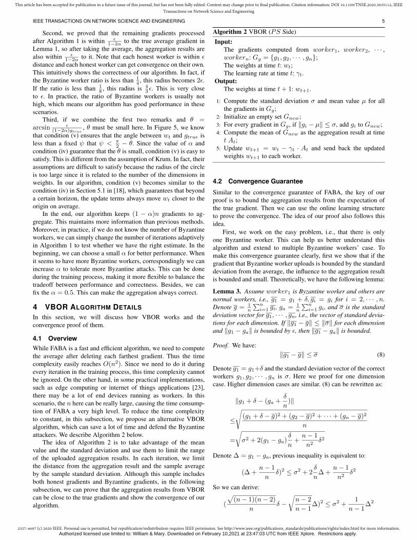
4 VBOR ALGORITHM DETAILS

In this section, we will discuss how VBOR works and theconvergence proof of them.

4.1 OverviewWhile FABA is a fast and efficient algorithm, we need to computethe average after deleting each farthest gradient. Thus the timecomplexity easily reaches O(n2). Since we need to do it duringevery iteration in the training process, this time complexity cannotbe ignored. On the other hand, in some practical implementations,such as edge computing or internet of things applications [23],there may be a lot of end devices running as workers. In thisscenario, the n here can be really large, causing the time consump-tion of FABA a very high level. To reduce the time complexityto constant, in this subsection, we propose an alternative VBORalgorithm, which can save a lot of time and defend the Byzantineattackers. We describe Algorithm 2 below.

The idea of Algorithm 2 is to take advantage of the meanvalue and the standard deviation and use them to limit the rangeof the uploaded aggregation results. In each iteration, we limitthe distance from the aggregation result and the sample averageby the sample standard deviation. Although this sample includesboth honest gradients and Byzantine gradients, in the followingsubsection, we can prove that the aggregation results from VBORcan be close to the true gradients and show the convergence of ouralgorithm.

Algorithm 2 VBOR (PS Side)

Input:The gradients computed from worker1, worker2, · · · ,workern: Gg = {g1, g2, · · · , gn};The weights at time t: wt;The learning rate at time t: γt.

Output:The weights at time t+ 1: wt+1.

1: Compute the standard deviation σ and mean value µ for allthe gradients in Gg;

2: Initialize an empty set Gnew;3: For every gradient in Gg , if ‖gi − µ‖ ≤ σ, add gi to Gnew;4: Compute the mean of Gnew as the aggregation result at timet At;

5: Update wt+1 = wt − γt · At and send back the updatedweights wt+1 to each worker.

4.2 Convergence Guarantee

Similar to the convergence guarantee of FABA, the key of ourproof is to bound the aggregation results from the expectation ofthe true gradient. Then we can use the online learning structureto prove the convergence. The idea of our proof also follows thisidea.

First, we work on the easy problem, i.e., that there is onlyone Byzantine worker. This can help us better understand thisalgorithm and extend to multiple Byzantine workers’ case. Tomake this convergence guarantee clearly, first we show that if thegradient that Byzantine worker uploads is bounded by the standarddeviation from the average, the influence to the aggregation resultis bounded and small. Theoretically, we have the following lemma:

Lemma 3. Assume worker1 is Byzantine worker and others arenormal workers, i.e., g1 = g1 + δ, gi = gi for i = 2, · · · , n.Denote g = 1

n

∑ni=1 gi, ga = 1

n

∑ni=1 gi, and σ is the standard

deviation vector for g1, · · · , gn, i.e., the vector of standard devia-tions for each dimension. If ‖g1 − g‖ ≤ ‖σ‖ for each dimensionand ‖g1 − ga‖ is bounded by ε, then ‖g1 − ga‖ is bounded.

Proof. We have:‖g1 − g‖ ≤ σ (8)

Denote g1 = g1+δ and the standard deviation vector of the correctworkers g1, g2, · · · , gn is σ. Here we proof for one dimensioncase. Higher dimension cases are similar. (8) can be rewritten as:

‖g1 + δ − (ga +δ

n)‖

≤

√(g1 + δ − g)2 + (g2 − g)2 + · · ·+ (gn − g)2

n

=

√σ2 + 2(g1 − ga)

δ

n+n− 1

n2δ2

Denote ∆ = g1 − ga, previous inequality is equivalent to:

(∆ +n− 1

nδ)2 ≤ σ2 + 2

δ

n∆ +

n− 1

n2δ2

So we can derive:

(

√(n− 1)(n− 2)

nδ −

√n− 2

n− 1∆)2 ≤ σ2 +

1

n− 1∆2





which is equivalent to:

‖√

(n− 1)(n− 2)

nδ −

√n− 2

n− 1∆‖ ≤

√σ2 +

1

n− 1∆2

This means:

‖δ‖ ≤ ‖ n

n− 1∆‖+

n√(n− 1)(n− 2)

√σ2 +

1

n− 1∆2

In the end, let η = n√(n−1)(n−2)

, we have:

‖g1 − ga‖ ≤ ‖δ‖+ ‖∆‖

≤ ‖2n− 1

n− 1∆‖+ η

√σ2 +

1

n− 1∆2 (9)

Since ∆ is bounded, ‖g1 − ga‖ is bound.

With the help of Lemma 3, we can extend this bound betweenaggregation results and expectation of the true gradients to multi-ple Byzantine worker cases. Theoretically, we have Lemma 4.

Lemma 4. Assume worker1, · · · , workerk are Byzantine work-ers and others are normal workers, i.e., gi = gi + δi for i =1, 2, · · · , k, gi = gi for i = k+ 1, · · · , n. If ‖gi− g‖ ≤ ‖σ‖ foreach dimension and ‖gi−ga‖ is bounded by ε for i = 1, 2, · · · , k,then ‖gi − ga‖ is bounded.

Proof. Denote ∆i = gi − ga for i = 1, 2, · · · , n and g(i)a =(g1 + · · ·+ gi−1 + gi + gi+1 + · · ·+ gk + gk+1 + · · ·+ gn)/nfor i = 1, 2, · · · , k. From Lemma 3, we know that:

‖gi − g(i)a ‖ ≤ ‖2n− 1

n− 1∆i‖+ η

√σ2 +

1

n− 1∆2i (10)

If we denote δm = maxi ‖δi‖, from triangle inequality, we have:

‖gi − ga‖ ≤‖gi − g(i)a ‖+ ‖g(i)a − ga‖

≤‖2n− 1

n− 1∆i‖+ η

√σ2 +

1

n− 1∆2i

+ ‖δ1 + · · ·+ δi−1 + δi+1 + · · ·+ δkn

‖

≤‖2n− 1

n− 1∆i‖+ η

√σ2 +

1

n− 1∆2i + ‖n− 1

nδm‖

Without loss of generality, we assume l = arg maxi δi, then wehave:

‖gl − ga‖ ≤ ‖2n− 1

n− 1∆l‖+ η

√σ2 +

1

n− 1∆2l + ‖n− 1

nδl‖

From triangle inequality, we have:

‖gl − gl‖ ≤‖gl − ga‖+ ‖2n− 1

n− 1∆l‖+ η

√σ2 +

1

n− 1∆2l

+ ‖n− 1

nδl‖ (11)

(11) is equivalent to:

‖δl‖ ≤n(‖∆l‖+ ‖2n− 1

n− 1∆l‖+ η

√σ2 +

1

n− 1∆2l )

=‖3n− 2

n− 1∆l‖+ η

√σ2 +

1

n− 1∆2l (12)

From the definition of l, we know that ‖δi‖ < ‖δl‖ for i =1, 2, · · · , k. Then we have:

‖gi − ga‖ ≤‖gi − gi‖+ ‖gi − ga‖ = ‖δi‖+ ‖∆i‖

≤‖3n− 2

n− 1∆l‖+ η

√σ2 +

1

n− 1∆2l + ‖∆i‖ (13)

≤‖4n− 3

n− 1ε‖+ η

√σ2 +

1

n− 1ε2 (14)

Since ∆i and ∆l are bounded, ‖gi − ga‖ is bound.

Because ga is an unbiased estimate of E‖G‖, while G is thedistribution of the correct workers’ gradient, from Lemma 4, weknow that as long as a worker’s uploaded gradients are bounded,no matter whether it is Byzantine, the distance between thesegradients to E‖G‖ is also bounded.

Lemma 5. We choose average function as A(·) to make ag-gregation, and it satisfies all the conditions from Lemma 4, ifthere exists an constant C > 0, s.t. ε < C · ga, then we havefor r = 2, 3, 4, E‖A‖r is bounded by a linear combination ofE‖G‖r1 , · · · , E‖G‖rm with r1 + · · ·+ rm = r.

Proof. We have:

‖A‖ = ‖ 1

n(g1 + · · ·+ gk + · · ·+ gn)‖

By triangle inequality,

‖A‖ ≤ 1

n(‖g1‖+ ·+ ‖gn‖) +

k

nε

≤ 1

n

∑i

‖gi‖+kC

n‖ga‖

So we have:

‖A‖r ≤ C0

∑r1+···+rn+1=r

‖g1‖r1 · · · ‖gn‖rn‖ga‖rn+1

for proper constant C0. This implies E‖A‖r is bounded bya linear combination of E‖g1‖r1 · · ·E‖gn‖rnE‖ga‖rn+1 =E‖G‖r1 · · ·E‖G‖rnE‖G‖rn+1 with r1 + · · ·+ rn+1 = r.

From Lemma 4 and Lemma 5, similar to the proof of FABA,we have the following Theorem 3 to ensure the convergence.

Theorem 3. We assume that (i) the cost function cost(w) is threetimes differentiable with continuous derivatives and non-negative;(ii) the learning rates satisfy

∑t γt = ∞ and

∑t γ

2t < ∞; (iii)

the gradients estimator satisfies EG = ∇Cost(w) and ∀r =2, 3, 4, E||G||r ≤ Ar + BR||w||r for some constants Ar , Br;(iv) ε < C · ||G|| and C is a relatively small constant that is lessthan 1; (v) let θ = arcsin (‖ 4n−3n−1 ε‖+ η

√σ2 + 1

n−1ε2)/gtrue,

beyond the surface ||w||2 > D, there exists e > 0 and 0 ≤ ψ <π2 − θ, s.t.

||∇Cost(w)|| ≥ e > 0

〈w,∇Cost(w)〉||w|| · ||∇Cost(w)||

≥ cosψ

Then the sequence of gradients ∇Cost(wt) converges almostsurely to 0.





0 20 40 60 80epochs

0.4

0.5

0.6

0.7

0.8

accu

racy

Gaussian

0 20 40 60 80epochs

0.4

0.5

0.6

0.7

0.8

accu

racy

Wrong Label

0 20 40 60 80epochs

0.4

0.5

0.6

0.7

0.8

accu

racy

One Bit

Krum GeoMedian FABA VBOR No Byzantine

Fig. 2: Experiment results of different algorithms for Gaussian, wrong label and one bit Byzantine attacks on CIFAR-10 for 8 workers

0 20 40 60 80epochs

0.88

0.90

0.92

0.94

0.96

0.98

accu

racy

Gaussian

0 20 40 60 80epochs

0.86

0.88

0.90

0.92

0.94

0.96

0.98

accu

racy

Wrong Label

0 20 40 60 80epochs

0.90

0.92

0.94

0.96

0.98

accu

racy

One Bit


Fig. 3: Experiment results of different algorithms for Gaussian, wrong label and one bit Byzantine attacks on MNIST for 8 workers

4.3 Remarks

Similar to FABA, VBOR is also based on the gradients locationinformation. However, there are several differences.

First, the time complexity of VBOR is O(n), and the timecomplexity of FABA is O(n2). This does not make a very hugedifference when n is small. However, in some large scale appli-cations, such as distributed machine learning on edge computing,n can be relatively large. In this scenario, we still need to do thisalgorithm in PS in every iteration. The time difference can bereally large.

Second, In VBOR, we also need to assume that all the truegradients are close. As we talked in Section 3.3, this needs allthe assigned datasets satisfying the same distribution and the minibatch size in each worker is sufficiently large. This is very easy toachieve in practice.

Third, the convergence speed in VBOR may be not as goodas FABA. In VBOR, we remove the outliers by the mean andvariance value, this makes it very possible to remove byzantinegradients along with some gradients that are from the honestworkers. Thus, in one iteration, FABA can keep more informationthan VBOR, making it converge faster than VBOR. However,FABA has one more hyperparameter than VBOR: the assumedproportion of Byzantine workers α. We need to manually tune thisparameter based on the estimate of Byzantine workers during thetraining. Although it is possible to tune it by designing auxiliaryalgorithms to help tune this parameter in the training process, it isnot as convenient as VBOR.

In the end, apart from using σ as the bound, in VBOR we canalso change it to c · σ as the bound to remove the outliers. Whenthe proportion of Byzantine workers is small, we can choose alarge c value to accelerate the training process.

5 EXPERIMENT

In this section, we are going to run our FABA and VBOR ina simulated Byzantine environment on MNIST dataset [19] andCIFAR-10 dataset [21].

In our experiment, we conduct three different type attacks. Thefirst is the Gaussian attack. We simply generate Gaussian noise asattack gradients and weights. The second method is wrong labeledattack. We let the label of the Byzantine workers’ data randomlyplaced, then the Byzantine worker just normally computes thegradient and weight, and upload results with wrong labeled data toPS. The last method is one bit attack. For the uploaded gradientand weight, we only change one dimension of it with randomvalue. For the comparison, we compare FABA and VBOR withtwo state-of-the-art algorithms: score-based algorithm Krum [12]and median-based algorithm GeoMedian [15]. In the experiments,we train our model on a distributed environment with 4 NvidiaGeForce GTX 1080Ti GPUs. In most of the experiments, weset the number of workers to 8, which means each GPU has 2workers. We choose LeNet-5 [19] as the neural network to trainon MNIST dataset and ResNet-18 [2] as the model to train onCIFAR-10 dataset. LeNet-5 is trained by a SGD optimizer with0.5 as momentum and 0.01 as learning rate. ResNet-18 is trainedby a SGD optimizer with 0.5 as momentum, 5× 10−4 as weightdecay and 0.01 as learning rate. The batch size for both neuralnetworks is set to 64. We train all the experiments for 80 epochs.

5.1 Algorithm Comparison

5.1.1 8-Worker Environment

We compare FABA and VBOR with Krum, GeoMedian and noByzantine scenario on three types of attacks that we describedbefore for both MNIST and CIFAR-10 dataset. We have 8 total





0 20 40 60 80epochs

0.6

0.7

0.8

0.9

1.0

accu

racy

Gaussian

0 20 40 60 80epochs

0.2

0.4

0.6

0.8

1.0

accu

racy

Wrong Label

0 20 40 60 80epochs

0.6

0.7

0.8

0.9

1.0

accu

racy

One Bit


Fig. 4: Experiment results of different algorithms for Gaussian, wrong label and one bit Byzantine attacks on MNIST for 32 workers

workers, among which 2 workers are Byzantine workers. Theexperiment results are in Figure 2, Figure 3.

As we can see from Figure 2, FABA and VBOR convergemuch faster than GeoMedian and Krum, and the performance ismore stable. Their performance can almost be the same or evenbeat a little bit compared to the no Byzantine case for all the threetypes of attacks. GeoMedian and Krum can also resist all the threetypes of attacks, but the convergence speed is much slower thanour algorithms. For MNIST dataset, the results are similar. We cansee from Figure 3 that FABA and VBOR outperforms GeoMedianand Krum for all kinds of attacks, while GeoMedian has slightlybetter performance than Krum.

5.1.2 32-Worker EnvironmentBecause of the limitation of the hardware, we cannot deploy anenvironment with more workers on CIFAR-10 dataset. Thus weonly deploy a 32-worker environment on MNIST dataset. EachGPU holds 8 workers. We use the same setting as the 8-workerenvironment. This time we changed the number of Byzantineworkers to 9. The results are shown in Figure 4.

The results from Figure 4 are very similar to the 8-workerenvironment. FABA and VBOR have better convergence speedand performance than GeoMedian and Krum, while GeoMedianis slightly better than Krum.

5.2 Byzantine Worker Ratio Comparison

The ratio of Byzantine workers can be very different. In thissection, we are going to compare the performance change ofdifferent Byzantine worker ratios. We still choose to deploy onan 8-worker environment for both CIFAR-10 and MNIST dataset.We choose the number of Byzantine workers to be 1, 2, and 3,which respectively implies the ratio of Byzantine workers 0.125,0.25, and 0.375. The performances for the comparison betweenFABA, VBOR and Krum, GeoMedian are similar. So here we onlyshow the performance of FABA and VBOR for different Byzantineworker ratios in Table 1.

Byzantine ratio 0.125 0.25 0.375

FABAGaussian 99.11% 99.15% 99.09%

Wrong Label 99.07% 99.05% 99.10%One Bit 98.97% 98.73% 98.25%

VBORGaussian 99.11% 99.07% 99.13%

Wrong Label 99.09% 99.04% 99.10%One Bit 98.87% 98.64% 98.35%

TABLE 1: The best accuracy performance of different Byzantineworker ratios on different attacks for FABA and VBOR

From this table we can see that as the Byzantine workerratio increases, for all three types of attacks, the performancedoes not vary much. This shows that our algorithms are capableof defending Byzantine attacks in different ratios of Byzantineworkers.

5.3 Time Complexity ComparisonWe compare the time complexity for FABA, VBOR, GeoMedianand Krum on MNIST dataset and CIFAR-10 dataset. For MNIST,we use a 32 worker environment with 9 Byzantine workers. ForCIFAR-10, we use an 8-worker environment with 2 Byzantineworkers. The time consumption results are in Table 2.

Algorithm Krum GeoMedian FABA VBORMNIST

Gaussian 11613.7s 23125.2s 4447.9s 3214.1sWrong Label 12025.3s 24276.2s 3697.3s 3264.5s

One Bit 11632.4s 24098.5s 4008.4s 3333.3sCIFAR-10

Gaussian 6291.5s 10112.7s 5245.7s 5164.8sWrong Label 5762.7s 9893.2s 5188.8s 5343.9s

One Bit 6663.3s 11863.9s 6080.4s 6036.0s

TABLE 2: The time complexity of different algorithms on differentattacks for MNIST and CIFAR-10

From Table 2, we can see that VBOR is the most efficientalgorithm compared to FABA, Krum and GeoMedian. When thenumber of workers is small, VBOR, FABA and Krum have similarperformance on time consumption. However, when the number ofworkers increases, VBOR performs much better than all otheralgorithms, and FABA has second best efficiency performance.GeoMedian is the slowest algorithm because it adopts an iterativemethod to find the geometric median.

6 CONCLUSION

As distributed neural networks become much more popular andare being used more widely, people are beginning to enjoy theefficiency and effectiveness brought by neural networks. However,such networks are also subject to Byzantine attacks. In this paper,we proposed two effective outlier deletion based algorithms FABAand VBOR to resist the Byzantine attacks in distributed neuralnetworks. We proved the convergence of our algorithms. In fact,in our algorithms, we can ensure that the aggregated results arevery close to the true gradients. Our algorithms are more efficientbecause we use as much information as we can in all uploadedgradients. We take the average of all rest gradients and use it





as aggregated results. Experiments demonstrate that our algorithmcan achieve approximately the similar speed and accuracy as in thenon-Byzantine settings, and the performance is much better thanpreviously proposed methods. Besides, FABA is easy to constructand control, making it simple to change how many Byzantinegradients that we want to delete by changing the parametersthrough the training process. VBOR has a smaller time complexitywith only little accuracy loss and also is very easy to implement.We believe that our easy and original algorithms can be widelyused in distributed neural networks to protect against Byzantineattacks.

ACKNOWLEDGEMENTS

This project was supported in part by US National ScienceFoundation grant CNS-1816399. This work was also supportedin part by the Commonwealth Cyber Initiative, an investment inthe advancement of cyber R&D, innovation and workforce devel-opment. For more information about CCI, visit cyberinitiative.org.

APPENDIXPROOF OF THEOREM 2

Proof. This proof follows Bottou’s proof in [18] and the proofof Proposition 2 in the supplementary material of [12] with somemodifications.

Condition (v) is complicated, so we use Figure 5 to clarify it.The dotted circle means the ball that all honest gradients lie in.

θ

ψ

Wt

At

gtrue

ε/(1-2α)

ε

Fig. 5: Condition (v)

By Lemma 1, At is in the ball whose center is gtrue and radiusis ε

1−2α . This assumption means that the angle between wt andgtrue is less than ψ while ψ < π

2 − θ.We start with showing the global confinement within the

region ||w|| ≤ D.(Global confinement). Let

φ(x) =

{0 if x < D

(x−D)2 otherwise

We denote ut = φ(||wt||2).Because φ has the property that

φ(y)− φ(x) ≤ (y − x)φ′(x) + (y − x)2 (15)

We have

ut+1 − ut ≤ (−2γt〈wt, At〉+ γ2t ||At||2) · φ′(||wt||2)

+ 4γ2t 〈wt, At〉2 − 4γ3t 〈wt, At〉||At||2 + γ4t ||At||4

≤ −2γt〈wt, At〉φ′(||wt||2) + γ2t ||At||2φ′(||wt||2)

+ 4γ2t ||wt||2||At||2 + 4γ3t ||wt||||At||3 + γ4t ||At||4

Denote %t as the σ-algebra that represents the information in timet. We can get the conditional expectation as

E(ut+1 − ut|%t)≤− 2γt〈wt, EAt〉+ γ2tE(||At||2)φ′(||wt||2)

+4γ2t ||wt||2E(||At||2) + 4γ3t ||wt||E(||At||3) + γ4tE(||At||4)

By Lemma 2, there exist positive constants X0, Y0, X, Y suchthat

E(ut+1 − ut|%t) ≤− 2γt〈wt, EAt〉φ′(||wt||2)

+ γ2t (X0 + Y0||wt||4)

≤− 2γt〈wt, EAt〉φ′(||wt||2)

+ γ2t (X + Y · ut)

The first term in the right is 0 when ||wt||2 < D. When ||wt||2 ≥D, because of Figure 5, we have

〈wt, EAt〉 ≥ ||wt|| · ||EAt|| · cos(θ + ψ) > 0

So we have

E(ut+1 − ut|%t) ≤ γ2t (X + Y · ut) (16)

For the following proof we define two auxiliary sequences µt =∏t−1i=1

11+γ2

i Y−−−→t→∞

µ∞ and u′t = µtut.

Because of (16), we can move γ2t Y · ut to the left and we get

E(u′t+1 − u′t|%t) ≤ γ2t µtX

Define an indicator function χt as

χt =

{1 E(u′t+1 − u′t|%t) > 0

0 otherwise

Then we have

E(χt(u′t+1 − u′t)) ≤ E(χt(u

′t+1 − u′t|%t))

≤ γ2t µtX (17)

By the quasi-martingale convergence theorem [24], (17) impliesthat the sequence u′t converges almost surely, which also impliesthat ut converges almost surely, that is, ut → u∞.

If we assume u∞ > 0, when t is large enough, we have||wt||2 > D and ||wt+1||2 > D, so (15) becomes an equality.This means that

∞∑t=1

γt〈wt, EAt〉φ′(||wt||2) <∞

Since we have φ′(||wt||2) converge to a positive value and in theregion ||wt||2 > D, by the condition (iv) and (v), we have

〈wt, EAt〉 ≥√D||EAt|| cos(θ + ψ)

≥√D(||∇Cost(wt)|| −

ε

1− 2α) cos(θ + ψ) > 0

This contradicts the condition (ii). So we have the ut converge to0, which gives the global confinement that ||wt|| is bounded. As aresult, any continuous function of wt is bounded.

(Convergence) Here we are going to show that ∇Cost(wt)converges almost surely to 0. First we denote ht = Cost(wt).If we use first order Taylor expansion and bound second orderderivatives with K1, we have

|ht+1 − ht + 2γt〈At,∇Cost(wt)〉| ≤ γ2t ||At||2K1 a.s.





This implies that

E(ht+1 − ht|%t) ≤ −2γt〈EAt,∇Cost(wt)〉+ γ2tE(||At||2|%)K1 (18)

≤ γ2tK2K1

This also shows thatE(χt(ht+1−ht)) ≤ γ2tK2K1. By the quasi-martingale convergence theorem, ht converges almost surely, thatis, Cost(wt)→ Cost∞. If we move the negative part to the left,take expectation of both sides and sum them for t, we get

∞∑t=1

γt〈EAt,∇Cost(wt)〉 <∞ a.s.

Next we denote ρt = ||∇Cost(wt)||2. If we use first orderTaylor expansion and bound second order derivatives with K3, wehave

ρt+1 − ρt ≤− 2γt〈At,∇2Cost(wt) · ∇Cost(wt)+ γ2t ||At||2K3

Taking conditional expectation of both side and bounding thesecond derivatives by K4, we have

E(ρt+1 − ρt|%t) ≤ 2γt〈EAt,∇Cost(wt)〉K4 + γ2tK2K3

This implies that

E(χt(ρt+1 − ρt)) ≤ 2γt〈EAt,∇Cost(wt)〉K4 + γ2tK2K3

By the quasi-martingale convergence theorem, this shows that ρtconverges almost surely.

We have

〈EAt,∇Cost(wt)〉

≥(||∇Cost(wt)|| −ε

1− 2α) · ||∇Cost(wt)||

≥(1− sin θ) · ρtThis implies that

∑∞t=1 γt · ρt < ∞ a.s.. Because condition

(ii) and ρt converges almost surely, we have that the sequence||∇Cost(wt)|| converges almost surely to 0.

REFERENCES

[1] L. J. Ba and R. Caurana, “Do deep nets really need tobe deep?” CoRR, vol. abs/1312.6184, 2013. [Online]. Available:http://arxiv.org/abs/1312.6184

[2] Kaiming He, Xiangyu Zhang, Shaoqing Ren, and Jian Sun, “Deepresidual learning for image recognition,” in 2016 IEEE Conference onComputer Vision and Pattern Recognition (CVPR), June 2016, pp. 770–778.

[3] Jia Deng, Wei Dong, Richard Socher, Li-jia Li, Kai Li, and Li Fei-Fei,“Imagenet: A large-scale hierarchical image database,” in 2009 IEEEConference on Computer Vision and Pattern Recognition, June 2009, pp.248–255.

[4] Norman P. Jouppi, Cliff Young, and N. et al., “In-datacenter performanceanalysis of a tensor processing unit,” in 2017 ACM/IEEE 44th AnnualInternational Symposium on Computer Architecture (ISCA), June 2017,pp. 1–12.

[5] N. S. Keskar, D. Mudigere, J. Nocedal, M. Smelyanskiy, and P. T. P.Tang, “On large-batch training for deep learning: Generalization gap andsharp minima,” CoRR, vol. abs/1609.04836, 2016. [Online]. Available:http://arxiv.org/abs/1609.04836

[6] J. Dean, G. S. Corrado, R. Monga, K. Chen, M. Devin, Q. V. Le, M. Z.Mao, M. Ranzato, A. Senior, P. Tucker, K. Yang, and A. Y. Ng, “Largescale distributed deep networks,” in Proceedings of the 25th InternationalConference on Neural Information Processing Systems - Volume 1,ser. NIPS’12. USA: Curran Associates Inc., 2012, pp. 1223–1231.[Online]. Available: http://dl.acm.org/citation.cfm?id=2999134.2999271

[7] M. Abadi, P. Barham, J. Chen, Z. Chen, A. Davis, J. Dean, M. Devin,S. Ghemawat, G. Irving, M. Isard, M. Kudlur, J. Levenberg, R. Monga,S. Moore, D. G. Murray, B. Steiner, P. Tucker, V. Vasudevan,P. Warden, M. Wicke, Y. Yu, and X. Zheng, “Tensorflow: A system forlarge-scale machine learning,” in Proceedings of OSDI, ser. OSDI’16.Berkeley, CA, USA: USENIX Association, 2016, pp. 265–283. [Online].Available: http://dl.acm.org/citation.cfm?id=3026877.3026899

[8] S. Yi, C. Li, and Q. Li, “A survey of fog computing: Concepts,applications and issues,” in Proceedings of the 2015 Workshop onMobile Big Data, ser. Mobidata ’15. New York, NY, USA: Associationfor Computing Machinery, 2015, p. 37–42. [Online]. Available:https://doi.org/10.1145/2757384.2757397

[9] S. Yi, Z. Hao, Z. Qin, and Q. Li, “Fog computing: Platform andapplications,” in Proceedings of the 2015 Third IEEE Workshop on HotTopics in Web Systems and Technologies (HotWeb), ser. HOTWEB ’15.USA: IEEE Computer Society, 2015, p. 73–78. [Online]. Available:https://doi.org/10.1109/HotWeb.2015.22

[10] Z. Tao, Q. Xia, Z. Hao, C. Li, L. Ma, S. Yi, and Q. Li, “A survey of virtualmachine management in edge computing,” Proceedings of the IEEE, vol.107, no. 8, pp. 1482–1499, 2019.

[11] L. Lamport, R. Shostak, and M. Pease, “The byzantine generalsproblem,” ACM Trans. Program. Lang. Syst., vol. 4, no. 3, pp.382–401, Jul. 1982. [Online]. Available: http://doi.acm.org/10.1145/357172.357176

[12] P. Blanchard, E. M. El Mhamdi, R. Guerraoui, and J. Stainer,“Machine learning with adversaries: Byzantine tolerant gradientdescent,” in Advances in Neural Information Processing Systems30, I. Guyon, U. V. Luxburg, S. Bengio, H. Wallach, R. Fergus,S. Vishwanathan, and R. Garnett, Eds. Curran Associates, Inc.,2017, pp. 119–129. [Online]. Available: http://papers.nips.cc/paper/6617-machine-learning-with-adversaries-byzantine-tolerant-gradient-descent.pdf

[13] G. Damaskinos, E. M. El Mhamdi, R. Guerraoui, R. Patra, andM. Taziki, “Asynchronous Byzantine machine learning (the case ofSGD),” in Proceedings of the 35th International Conference onMachine Learning, ser. Proceedings of Machine Learning Research,J. Dy and A. Krause, Eds., vol. 80. Stockholmsmassan, StockholmSweden: PMLR, 10–15 Jul 2018, pp. 1145–1154. [Online]. Available:http://proceedings.mlr.press/v80/damaskinos18a.html

[14] C. Xie, O. Koyejo, and I. Gupta, “Generalized byzantine-tolerantSGD,” CoRR, vol. abs/1802.10116, 2018. [Online]. Available:http://arxiv.org/abs/1802.10116

[15] D. Yin, Y. Chen, K. Ramchandran, and P. Bartlett, “Byzantine-robustdistributed learning: Towards optimal statistical rates,” CoRR, vol.abs/1803.01498, 2018. [Online]. Available: http://arxiv.org/abs/1803.01498

[16] Y. Chen, L. Su, and J. Xu, “Distributed statistical machine learningin adversarial settings: Byzantine gradient descent,” Proc. ACM Meas.Anal. Comput. Syst., vol. 1, no. 2, pp. 44:1–44:25, Dec. 2017. [Online].Available: http://doi.acm.org/10.1145/3154503

[17] D. Alistarh, Z. Allen-Zhu, and J. Li, “Byzantine stochastic gradientdescent,” CoRR, vol. abs/1803.08917, 2018. [Online]. Available:http://arxiv.org/abs/1803.08917

[18] L. Bottou, “On-line learning in neural networks,” in On-line Learningand Stochastic Approximations, D. Saad, Ed. New York, NY, USA:Cambridge University Press, 1998, pp. 9–42. [Online]. Available:http://dl.acm.org/citation.cfm?id=304710.304720

[19] Yann Lecun, Leon Bottou, Yoshua Bengio, and Patrick Haffner,“Gradient-based learning applied to document recognition,” Proceedingsof the IEEE, vol. 86, no. 11, pp. 2278–2324, Nov 1998.

[20] K. Simonyan and A. Zisserman, “Very deep convolutional networksfor large-scale image recognition,” CoRR, vol. abs/1409.1556, 2014.[Online]. Available: http://arxiv.org/abs/1409.1556

[21] A. Krizhevsky, “Learning multiple layers of features from tiny images,”Department of Computer Science, University of Toronto, Tech. Rep.,2009.

[22] X. Li, M. C. Huang, K. Shen, and L. Chu, “A realistic evaluationof memory hardware errors and software system susceptibility,”in Proceedings of the 2010 USENIX Conference on USENIXAnnual Technical Conference, ser. USENIXATC’10. Berkeley, CA,USA: USENIX Association, 2010, pp. 6–6. [Online]. Available:http://dl.acm.org/citation.cfm?id=1855840.1855846

[23] X. Li, R. Lu, X. Liang, X. Shen, J. Chen, and X. Lin, “Smart community:an internet of things application,” IEEE Communications Magazine,vol. 49, no. 11, pp. 68–75, 2011.

[24] M. Metivier, Semimartingales: a course on stochastic processes. Walterde Gruyter, 2011, vol. 2.


http://arxiv.org/abs/1312.6184


http://dl.acm.org/citation.cfm?id=2999134.2999271


https://doi.org/10.1145/2757384.2757397

https://doi.org/10.1109/HotWeb.2015.22

http://doi.acm.org/10.1145/357172.357176

http://doi.acm.org/10.1145/357172.357176

http://papers.nips.cc/paper/6617-machine-learning-with-adversaries-byzantine-tolerant-gradient-descent.pdf



http://proceedings.mlr.press/v80/damaskinos18a.html




http://doi.acm.org/10.1145/3154503





defenses against byzantine attacks in distributed deep

Documents