WATER DEFICIT VS WATER EXCESS

Alejandro Marulanda Aguirre

Civil Engineer, Hydraulic and Environmental Engineering.

Candidate M.Sc Hydraulic Resources.

Coauthors:

Jorge Julián Vélez U. Ph.D Hydrology

Olga Lucia Ocampo L. PhDc Engineering

Universidad Nacional de Colombia - Manizales

▪ Introduction

▪ Objectives

▪ Context

- Climate context

- Climate extremes: Wet and Dry

- Causes, effects and impacts

▪ Methodology

- Use of ArcGis in water supply

▪ Results

▪ Conclusions

AGENDA

Fresh water

Hydraulic infrastructure

Water demand

INTRODUCTION

Topic: Predicting Water Supply

OBJECTIVES

General objective

Estimate the water deficit hazard in municipal aqueducts with

water supply problems in the department of Caldas,

Colombia.

Specific objectives

1. Define a methodology to estimate the aqueduct water

supply.

2. Explain climate variability effects.

CONTEXT

ITCZ

ENSO

(Pacífico) Orinoquía

y Amazonía

Climate context in Colombia, South America:

National climate context:Influence of the Andes Mountains on Colombia, South America

Source: Gifex-HIMC, 2007. IDEAM, 2010.

Caldas

Altitud m.a.s.l.Annual precipitation

Caldas

CONTEXT

National climate context:

Source: IDEAM, 2010.

Annual Precipitation

Legend (mm) (In)

0 - 500 0 - 19,7

500 - 1000 19,7 - 39

1000 - 1500 39 - 59

1500 - 2000 59 - 79

2000 - 2500 79 - 98

2500 - 3000 98 - 118

3000 - 4000 118 - 158

4000 - 5000 158 - 197

5000 - 7000 197 - 276

7000 - 9000 276 - 354

9000 - 11000 354 - 433

> 11000 > 433

Caldas

Annual precipitation

CONTEXT

J F M A M J A S O N D

Source: CORPOCALDAS & Gotta, 2017.

Altitude Annual precipitation

Legend (mm) (In)

660 – 1000 26 – 39

1000 – 1500 39 – 59

1500 – 2500 59 – 98

2500 – 4000 98 – 157

4000 – 6000 157 – 236

> 6000 > 236

Legend m.a.s.l Feet

5289 208

141 5,5

CONTEXT

Local climate context – Caldas, Colombia:

Climate extremes:

Flow changes in the aqueduct water supply.

Fuente: CORPOCALDAS, 2017.

MUNICIPIO DE PENSILVANIA (EXP. 0640 )

MES DE JULIO DE 2014 MES DE ABRIL DE 2015

Quebrada El Dorado

Caudal de la Fuente: 120,5 l/s Caudal de la Fuente: 91 l/s

Caudal Captado: 18 l/s Caudal Captado: 18,84 l/s

REGISTRO FOTOGRÁFICO

Quebrada El Popal

Quebrada El Popal

Quebrada El Dorado

Quebrada El Dorado

MUNICIPIO DE PENSILVANIA (EXP. 0640 )

MES DE JULIO DE 2014 MES DE ABRIL DE 2015

Quebrada El Dorado

Caudal de la Fuente: 120,5 l/s Caudal de la Fuente: 91 l/s

Caudal Captado: 18 l/s Caudal Captado: 18,84 l/s

REGISTRO FOTOGRÁFICO

Quebrada El Popal

Quebrada El Popal

Quebrada El Dorado

Quebrada El Dorado

Manizales Victoria Pensilvania

CONTEXT

Climate extremes:Sea Surface Temperature Anomaly vs Flow regime

Source: CORPOCALDAS, 2017. NOAA, 2018.

MUNICIPIO DE PENSILVANIA (EXP. 0640 )

MES DE JULIO DE 2014 MES DE ABRIL DE 2015

Quebrada El Dorado

Caudal de la Fuente: 120,5 l/s Caudal de la Fuente: 91 l/s

Caudal Captado: 18 l/s Caudal Captado: 18,84 l/s

REGISTRO FOTOGRÁFICO

Quebrada El Popal

Quebrada El Popal

Quebrada El Dorado

Quebrada El Dorado

MUNICIPIO DE PENSILVANIA (EXP. 0640 )

MES DE JULIO DE 2014 MES DE ABRIL DE 2015

Quebrada El Dorado

Caudal de la Fuente: 120,5 l/s Caudal de la Fuente: 91 l/s

Caudal Captado: 18 l/s Caudal Captado: 18,84 l/s

REGISTRO FOTOGRÁFICO

Quebrada El Popal

Quebrada El Popal

Quebrada El Dorado

Quebrada El Dorado

CONTEXT

Climate extremes:

Influence of the ENSO (El Niño South Oscillation)

Source: CORPOCALDAS & Gotta, 2017.

Date 23/08/02 05/07/92 01/07/87 30/06/87 04/07/92 10/07/97 29/06/87 22/08/02 03/07/92 09/07/97 08/07/97 02/07/92 28/06/87 07/07/97 08/07/91

Mínimum

Flow (L/s)37.3 37.9 38.2 38.3 38.3 38.4 38.7 38.7 38.7 38.8 39.2 39.2 39.3 39.6 39.7

ONI Index 0.9 0.4 1.2 1 0.7 1.6 1.2 0.9 1.6 1.6 1.6 0.4 1.2 1.6 0.7

CONTEXT

J F M A M J A S O N D

Pre

cip

ita

tio

n(m

m/m

es)

Causes, effects and impacts:ENSO: “Refers to the coherent and sometimes very strong year-to-

year variations in sea- surface temperatures, convective rainfall,

surface air pressure, and atmospheric circulation that occur across

the equatorial Pacific Ocean”.

Extreme dry: 1982, 1992, 1997, 2015

Extreme wet: 1988, 2000, 2007, 2010

Source: NOAA, 2018.

CONTEXT

Source: Wilhite, 2000.

CONTEXT

CONTEXT

METHODOLOGY

Integrated Water Resources Management (IWRM):

Colombia IWRM:

Source: MINAMBIENTE, 2017.

Supply Demand Quality Risk

Source: ICIWaRM, 2018.

METHODOLOGY

1• Climatic characterization

2• Flow regime

3• Flow recession curve

4• Flow probabilistic estimation

METHODOLOGY

1. Climatic characterization:

Standardised Precipitation Evapotranspiration Index (SPEI).

“The mean for a specified time period divided by the standard deviation

where the mean and standard deviation are determined from past records”.

0

0.2

0.4

0.6

0.8

1

-200 0 200 400 600 800 1000

F(X

)

Di

-200

0

200

400

600

800

1000

Di=

Pi-E

VP

i

-2

-1

0

1

2

3

SP

EI

-2

-1

0

1

2

3S

PE

I 1

MO

NT

H

Source: (McKee et al. 1993)

METHODOLOGY

2. Flow Regime: Measured or simulated flow

TETIS model (Francis et al 2007, Vélez, 2001)

RESULTS

8

13

18

23

280

20

40

60

80

100

01/01/81 21/11/86 10/10/92 30/08/98 19/07/04 08/06/10

T (

ºC)

P (

mm

)

DAILY Pmm Tmed°C

8

10

12

14

160

3000

6000

9000

12000

1 2 3 4 5 6 7 8 9 10 11 12

T (

ºC)

P (

mm

)

MULTI-YEAR MONTHLY Pmm Tmed°C

7

12

17

22

0

1500

3000

4500

1,981 1,984 1,987 1,990 1,993 1,996 1,999 2,002 2,005 2,008

T (

ºC)

P (

mm

)

ANNUAL Pmm Tmed°C

Climatic series:

RESULTS

Climatic characterization: (SPEI).

-3-2-10123

SP

EI

1 M

ON

TH

-2-10123

SP

EI

3 M

ON

TH

-3-2-10123

SP

EI

6 M

ON

TH

-2

-1

0

1

2

SP

EI

12 M

ON

TH

-2

-1

0

1

2

SP

EI

18 M

ON

TH

-2

-1

0

1

2

SP

EI

24 M

ON

TH

RESULTS

0

20

40

60

80

100

120

1400

5

10

15

20

25

Pre

cip

itat

ion

(m

m)

Flo

w r

ate

(m

3/s

) Qsimulado

Precipitación

Less rain, lower flow Higher rain, greater flow

Component Value Component Value

Static maximun storage 350,16 Surface storage 0

Conductivity (mm/day) 5,3 Infiltration exponent 2

Residence time - surface Flow (days) 3,79 Evaporation exponent 0,501

Gravitational storage 257

Hydrological modeling:

RESULTS

Location of rain stations:

RESULTS

Thiessen Polygons:

RESULTS

1ºC

13ºC

20ºC

0.5 mm

3.6 mm

5.9 mm

Precipitation

Temperature

Land cover

Land use

Source: IGAC, 2010

Inputs for hydrological model:

RESULTS

Digital Elevation Model (Sinks):

RESULTS

Flow Accumulation:

RESULTS

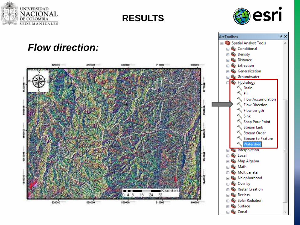
Flow direction:

RESULTS

Watershed delimitation:

METHODOLOGY

Tetis Model: Calibration and validation.Puente Juntas flow Station:

Costa Azul Station:

1981 – 1990

1991 – 2000

0

50

100

150

200

250

3000

10

20

30

40

50

60

P (

mm

)

Flo

wra

te(m

3/s

)

Qobservado

Qsimulado

050

100150200

2503000

10

203040

5060

P (

mm

)

Flo

wra

te(m

3/s

)

QobservadoQsimulado

0

50

100

150

200

250

3000

5

10

15

20

25

30

P (

mm

)

Flo

wra

te(m

3/s

)

QobservadoQsimulado

0

50

100

150

200

250

3000

5

10

15

20

25

30

P (

mm

)

Flo

wra

te(m

3/s

)

QobservadoQsimulado

RESULTS

Flow duration curve

0.0

0.2

0.4

0.6

0.8

1.0

1.2

1.4

1.6

1.8

2.0

0 10 20 30 40 50 60 70 80 90 100

Flo

wra

tem

3/s

Percentage Exceedance (%)

Q EL Uvito

Flow duration curve

P (%) Q0.01 Q1 Q10 Q25 Q50 Q65 Q75 Q85 Q90 Q95 Q97.5

Q (m³/s) 1.85 1.15 0.66 0.47 0.29 0.21 0.17 0.12 0.10 0.07 0.06

RESULTS

2. Flow Regime:

Supply vs Demand

0.00

0.05

0.10

0.15

0.20

0.25

0.30

0.35

0.40

0% 10% 20% 30% 40% 50% 60% 70% 80% 90% 100%

Flo

wra

te(L

/s)

Percentage Exceedance (%)

La Merced Aqueduct

Supply

Demand

RESULTS

Flow recession curve:

Theoretical:

Measure:

teQtQ 0

300

350

400

450

500

550

600

1 3 5 7 9

11

13

15

17

19

21

23

25

27

29

31

33

35

37

39

41

43

45

47

49

51

Flo

wra

te(L

/s)

Days without rain

Recession Rio Blanco, Manizales.Aguas de Manizales (Aqueduct)

JUN-10-JULIO-2015

RESULTS

Flow recession curve

y = -40.11ln(x) + 415.8R² = 0.9631

0

10

20

30

40

50

600.00

0.00

0.01

0.10

1.00

P (

mm

)

Flo

wra

te(m

3/s

) El Rosario

y = -9.53ln(x) + 99.884R² = 0.9506

0

10

20

30

40

50

600.00

0.01

0.10

1.00P

(m

m)

Flo

wra

te(m

3/s

)

Santana

y = -17.82ln(x) + 186.85R² = 0.9602

0

10

20

30

40

50

600.00

0.01

0.10

1.00

P (

mm

)

Flo

wra

te(m

3/s

)

Santana

y = -2.444ln(x) + 25.328R² = 0.9757

0

10

20

30

40

50

600.00

0.01

0.10

1.00

P (

mm

)

Flo

wra

te(m

3/s

) La Isabela

RESULTS

Flow probabilistic estimation:▪ Deficit: Normal, LogNormal and Gumbel.

▪ Excess: General Extreme Value GEV, Gumbel, Log-Normal, SQRT-

ETmax, Two Components Extreme Value TCEV.

Important situation for the supply: Accumulation of sediments and organic

material in drought season, with drag and swept of these with a medium or

maximum flow.

-0.1

0.0

0.1

0.2

0.3

0.4

0.5

0 10 20 30 40 50 60 70 80 90 100

Flo

wra

te(L

/s)

Return period (Year)

Probabilistic estimation of minimum flows

NORMAL

GUMBEL

LOGNORMAL

Rp (Year) Q (L/s)

2.33 0.3

5 0.2

10 0.1

25 0.06

50 0.04

100 0.03

Gumbel General Extreme

Value Rp (Year) Q (L/s)

2.33 24

5 32

10 48

25 80

50 160

100 240

Hydro-illogical cycle:

Source: Wilhite, 2000; National Drought Mitigation Center, 2018.

CONCLUSIONS

CONCLUSIONS

▪ It’s possible to estimate the hazard of shortage based

on the understanding of the associated natural

processes.

▪ The water regulation and retention not only depends

on the physical conditions (vegetation and soils) but it

is determined by the climate.

▪ The duration without rain is important in a deficit

event, while the magnitude is important in a excess

event due to the lag and event evolution.

CONCLUSIONS

▪ It’s important break a hydro-illogical cycle through risk

management (prevention and adaptation), ending with

crisis management (reactive).

▪ The vulnerability not only depends on the supply, also

on the quality of the water, the water demand and the

infrastructure for the supply.

▪ All flow regime is important to the supply. (adaptation

and mitigation measures).

Thanks!Alejandro Marulanda Aguirre

Contact: amarulandaa@unal.edu.co