definiens developer 7 - irfanakar.com definiens... · definiens developer 7 - reference book 3 ......
TRANSCRIPT

Definiens
Developer 7
Reference Book
Definiens AG
www.definiens.com

Definiens Developer 7 - Reference Book
2
Imprint and Version
Document Version 7.0.0.843
Copyright © 2007 Definiens AG. All rights reserved.
This document may be copied and printed only in accordance with the terms of the Frame License Agreement for End Users of the related Definiens software.
Published by
Definiens AG Trappentreustr. 1 D-80339 München Germany
Phone +49-89-231180-0 Fax +49-89-231180-90
E-mail [email protected] Web http://www.definiens.com
Dear User,
Thank you for using Definiens software. We appreciate being of service to you with image intelligence solutions.
At Definiens we constantly strive to improve our products. We therefore appreciate all comments and suggestions for improvements concerning our software, training, and documentation.
Feel free to contact us via web form on the Definiens support website http://www.definiens.com/support/index.htm.
Thank you.
Legal Notes
Definiens®, Definiens Cellenger® and Definiens Cognition Network Technology® are registered trademarks of Definiens AG in Germany and other countries. Cognition Network Technology™, Definiens eCognition™, Enterprise Image Intelligence™, and Understanding Images™, are trademarks of Definiens AG in Germany and other countries.
All other product names, company names, and brand names mentioned in this document may be trademark properties of their respective holders.
Protected by patents US 7146380, US 7117131, US 6832002, US 6738513, US 6229920, US 6091852, EP 0863485, WO 00/54176, WO 00/60497, WO 00/63788 WO 01/45033, WO 01/71577, WO 01/75574, and WO 02/05198. Further patents pending.
Definiens Developer 7 - Reference Book
3
Table of Contents
Developer 7 ____________________________________________________________ 1 Imprint and Version __________________________________________________ 2 Dear User, __________________________________________________________ 2 Legal Notes_________________________________________________________ 2
Table of Contents _______________________________________________________ 3 1 Introduction _______________________________________________________ 6 2 About Rendering a Displayed Image___________________________________ 7
2.1 About Image Layer Equalization __________________________________ 7 2.2 About Image Equalization _______________________________________ 8
3 Algorithms Reference ______________________________________________ 11 3.1 Process Related Operation Algorithms ___________________________ 13
3.1.1 Execute Child Processes 13 3.1.2 Set Rule Set Options 13
3.2 Segmentation Algorithms ______________________________________ 15 3.2.1 Chessboard Segmentation 15 3.2.2 Quad Tree Based Segmentation 16 3.2.3 Contrast Split Segmentation 18 3.2.4 Multiresolution Segmentation 21 3.2.5 Spectral Difference Segmentation 24 3.2.6 Contrast Filter Segmentation 25
3.3 Basic Classification Algorithms __________________________________ 28 3.3.1 Assign Class 28 3.3.2 Classification 28 3.3.3 Hierarchical Classification 29 3.3.4 Remove Classification 29
3.4 Advanced Classification Algorithms ______________________________ 29 3.4.1 Find Domain Extrema 30 3.4.2 Find Local Extrema 31 3.4.3 Find Enclosed by Class 33 3.4.4 Find Enclosed by Image Object 33 3.4.5 Connector 34 3.4.6 Optimal Box 35
3.5 Variables Operation Algorithms _________________________________ 37 3.5.1 Update Variable 37 3.5.2 Compute Statistical Value 39 3.5.3 Apply Parameter Set 40 3.5.4 Update Parameter Set 40
3.6 Reshaping Algorithms _________________________________________ 40 3.6.1 Remove Objects 40 3.6.2 Merge Region 40 3.6.3 Grow Region 41 3.6.4 Multiresolution Segmentation Region Grow 42 3.6.5 Image Object Fusion 43 3.6.6 Convert to Subobjects 46 3.6.7 Border Optimization 46 3.6.8 Morphology 47 3.6.9 Watershed Transformation 49
3.7 Level Operation Algorithms ____________________________________ 49 3.7.1 Copy Image Object Level 49 3.7.2 Delete Image Object Level 50 3.7.3 Rename Image Object Level 50
3.8 Training Operation Algorithms __________________________________ 50 3.8.1 Show User Warning 50
Definiens Developer 7 - Reference Book
4
3.8.2 Create/Modify Project 50 3.8.3 Update Action from Parameter Set 51 3.8.4 Update Parameter Set from Action 52 3.8.5 Manual Classification 52 3.8.6 Configure Object Table 52 3.8.7 Display Image Object Level 52 3.8.8 Select Input Mode 53 3.8.9 Activate Draw Polygons 53 3.8.10 Select Thematic Objects 53 3.8.11 End Thematic Edit Mode 54
3.9 Vectorization Algorithms_______________________________________ 54 3.10 Sample Operation Algorithms___________________________________ 54
3.10.1 Classified Image Objects to Samples 54 3.10.2 Cleanup Redundant Samples 55 3.10.3 Nearest Neighbor Configuration 55 3.10.4 Delete All Samples 55 3.10.5 Delete Samples of Class 55 3.10.6 Disconnect All Samples 55 3.10.7 Sample Selection 56
3.11 Image Layer Operation Algorithms_______________________________ 56 3.11.1 Create Temporary Image Layer 56 3.11.2 Delete Image Layer 56 3.11.3 Convolution Filter 57 3.11.4 Layer Normalization 58 3.11.5 Median Filter 60 3.11.6 Pixel Frequency Filter 60 3.11.7 Edge Extraction Lee Sigma 61 3.11.8 Edge Extraction Canny 62 3.11.9 Surface Calculation 63 3.11.10 Layer Arithmetics 64 3.11.11 Line Extraction 65 3.11.12 Apply Pixel Filters with Image Layer Operation Algorithms 66
3.12 Thematic Layer Operation Algorithms ____________________________ 66 3.12.1 Synchronize Image Object Hierarchy 67 3.12.2 Read Thematic Attributes 67 3.12.3 Write Thematic Attributes 67
3.13 Export Algorithms ____________________________________________ 67 3.13.1 Export Classification View 68 3.13.2 Export Current View 68 3.13.3 Export Thematic Raster Files 70 3.13.4 Export Domain Statistics 70 3.13.5 Export Project Statistics 71 3.13.6 Export Object Statistics 72 3.13.7 Export Object Statistics for Report 72 3.13.8 Export Vector Layers 73 3.13.9 Export Image Object View 74
3.14 Workspace Automation Algorithms ______________________________ 74 3.14.1 Create Scene Copy 74 3.14.2 Create Scene Subset 75 3.14.3 Create Scene Tiles 78 3.14.4 Submit Scenes for Analysis 78 3.14.5 Delete Scenes 80 3.14.6 Read Subscene Statistics 80
3.15 Customized Algorithms ________________________________________ 81 4 Features Reference ________________________________________________ 83
4.1 About Features as a Source of Information_________________________ 83 4.2 Basic Features Concepts _______________________________________ 83
4.2.1 Image Layer Related Features 84
Definiens Developer 7 - Reference Book
5
4.2.2 Image Object Related Features 87 4.2.3 Class-Related Features 91 4.2.4 Shape-Related Features 91 4.2.5 About Coordinate Systems 93 4.2.6 Distance-Related Features 94
4.3 Object Features ______________________________________________ 95 4.3.1 Customized 96 4.3.2 Layer Values 96 4.3.3 Shape 115 4.3.4 Texture 146 4.3.5 Variables 160 4.3.6 Hierarchy 161 4.3.7 Thematic Attributes 163
4.4 Class-Related Features________________________________________ 163 4.4.1 Customized 163 4.4.2 Relations to Neighbor Objects 164 4.4.3 Relations to Subobjects 168 4.4.4 Relations to Superobjects 170 4.4.5 Relations to Classification 171
4.5 Scene Features ______________________________________________ 173 4.5.1 Variables 173 4.5.2 Class-Related 173 4.5.3 Scene-Related 175
4.6 Process-Related Features______________________________________ 178 4.6.1 Customized 178
4.7 Customized ________________________________________________ 181 4.7.1 Largest possible pixel value 181 4.7.2 Smallest possible pixel value 181
4.8 Metadata __________________________________________________ 181 4.9 Feature Variables ____________________________________________ 182 4.10 Use Customized Features _____________________________________ 182
4.10.1 Create Customized Features 182 4.10.2 Arithmetic Customized Features 183 4.10.3 Relational Customized Features 185
4.11 Use Variables as Features______________________________________ 188 4.12 About Metadata as a Source of Information _______________________ 188 4.13 Table of Feature Symbols _____________________________________ 189
4.13.1 Basic Mathematical Notations 189 4.13.2 Images and Scenes 190 4.13.3 Image Objects Hierarchy 190 4.13.4 Image Object as a Set of Pixels 190 4.13.5 Bounding Box of an Image Object 191 4.13.6 Layer Intensity on Pixel Sets 191 4.13.7 Class Related Sets 191
5 Index ___________________________________________________________ 192

Definiens Developer 7 - Reference Book
6
1 Introduction
1 Introduction This Reference Book lists detailed information about algorithms and features, and provides general reference information. For individual image analysis and rule set development you may wish to keep a printout ready at hand.
Algorithms Reference on page 11
Features Reference on page 83
Definiens Developer 7 - Reference Book
7
2 About Rendering a DisplayedImage
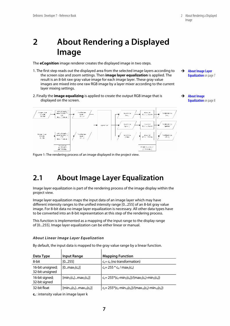
2 About Rendering a Displayed Image
The eCognition image renderer creates the displayed image in two steps.
1. The first step reads out the displayed area from the selected image layers according to the screen size and zoom settings. Then image layer equalization is applied. The result is an 8-bit raw gray value image for each image layer. These gray value images are mixed into one raw RGB image by a layer mixer according to the current layer mixing settings.
2. Finally the image equalizing is applied to create the output RGB image that is displayed on the screen.
Figure 1: The rendering process of an image displayed in the project view.
2.1 About Image Layer Equalization Image layer equalization is part of the rendering process of the image display within the project view.
Image layer equalization maps the input data of an image layer which may have different intensity ranges to the unified intensity range [0...255] of an 8-bit gray value image. For 8-bit data no image layer equalization is necessary. All other data types have to be converted into an 8-bit representation at this step of the rendering process.
This function is implemented as a mapping of the input range to the display range of [0...255]. Image layer equalization can be either linear or manual.
About Linear Image Layer Equalization
By default, the input data is mapped to the gray value range by a linear function.
Data Type Input Range Mapping Function 8-bit [0...255] cs= ck (no transformation)
16-bit unsigned; 32-bit unsigned
[0...max2(ck)] cs= 255 * ck / max2(ck)
16-bit signed; 32-bit signed
[min2(ck)...max2(ck)] cs= 255*(ck-min2(ck))/(max2(ck)-min2(ck))
32-bit float [min10(ck)...max10(ck)] cs= 255*(ck-min10(ck))/(max10(ck)-min10(ck))
ck : intensity value in image layer k
About Image Layer Equalization on page 7
About Image Equalization on page 8
Definiens Developer 7 - Reference Book
8
2 About Rendering a DisplayedImage
cs : intensity value on the screen
min2(ck) = max { x : x = -2n; x <= c'kmin } is the highest integer number that is a power of 2 and darker than the darkest actual intensity value of all pixel values of the selected layer.
max2(ck) = min { x : x = 2n; x >= c'kmax } is the lowest integer number that is a power of 2 and is brighter than the brightest actual intensity value of all pixel values of the selected layer.
min10(ck) = max { x : x = -10n; x <= c'kmin } is the highest integer number that is a power of 10 and darker than the darkest actual intensity value of all pixel values of the selected layer.
max10(ck) = min { x : x = 10n; x >= c'kmax } is the lowest integer number that is a power of 10 and is brighter than the brightest actual intensity value of all pixel values of the selected layer.
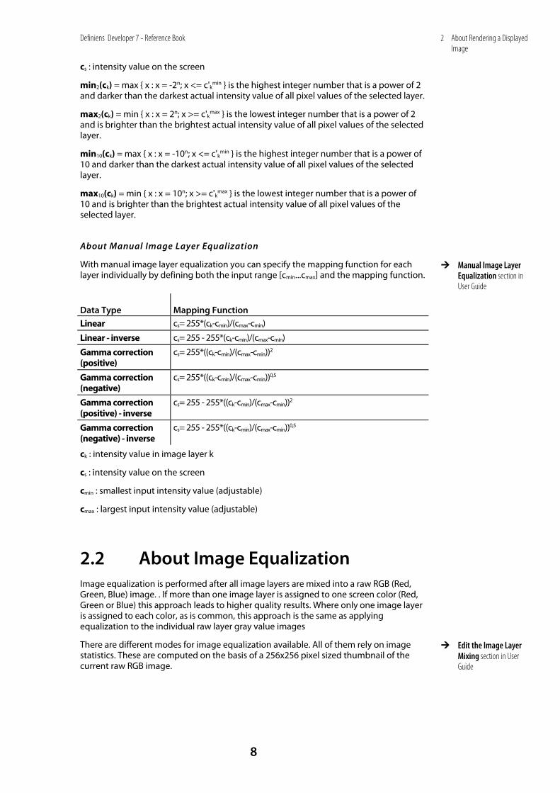
About Manual Image Layer Equalization
With manual image layer equalization you can specify the mapping function for each layer individually by defining both the input range [cmin...cmax] and the mapping function.
Data Type Mapping Function Linear cs= 255*(ck-cmin)/(cmax-cmin)
Linear - inverse cs= 255 - 255*(ck-cmin)/(cmax-cmin)
Gamma correction (positive)
cs= 255*((ck-cmin)/(cmax-cmin))2
Gamma correction (negative)
cs= 255*((ck-cmin)/(cmax-cmin))0,5
Gamma correction (positive) - inverse
cs= 255 - 255*((ck-cmin)/(cmax-cmin))2
Gamma correction (negative) - inverse
cs= 255 - 255*((ck-cmin)/(cmax-cmin))0,5
ck : intensity value in image layer k
cs : intensity value on the screen
cmin : smallest input intensity value (adjustable)
cmax : largest input intensity value (adjustable)
2.2 About Image Equalization Image equalization is performed after all image layers are mixed into a raw RGB (Red, Green, Blue) image. . If more than one image layer is assigned to one screen color (Red, Green or Blue) this approach leads to higher quality results. Where only one image layer is assigned to each color, as is common, this approach is the same as applying equalization to the individual raw layer gray value images
There are different modes for image equalization available. All of them rely on image statistics. These are computed on the basis of a 256x256 pixel sized thumbnail of the current raw RGB image.
Manual Image Layer Equalization section in User Guide
Edit the Image Layer Mixing section in User Guide

Definiens Developer 7 - Reference Book
9
2 About Rendering a DisplayedImage
None
No (None) equalization allows you to see the image data as it is, which can be helpful at the beginning of rule set development, when looking for an approach.
The output from the image layer mixing is displayed without further modification.
Input Range Mapping Function [0...255] [0...255]
Linear Equalization
Linear equalization with 1.00% is the default for new scenes. Commonly it displays images with a higher contrast as without image equalization.
Linear equalization maps each color Red, Green, and Blue (RGB) from an input range [cmin...cmax] to the available screen intensity range [0...255] by a linear mapping. The input range can be modified by the percentage parameter p. The input range is computed such that p percent of the pixels are not part of the input range. In case p=0 this means the range of used color values is stretched to the range [0....255]. For p>0 the mapping ignores p/2 percent of the darkest pixels and p/2 percent of the brightest pixels. In many cases a small value of p lead to better results because the available color range can be better used for the relevant data by ignoring the outliers.
cmin = max { c : #{ (x,y) : ck(x,y) < cmin} / (sx*sy) >= p/2 }
cmax = min { c : #{ (x,y) : ck(x,y) > cmax} / (sx*sy) >= p/2 }
Input Range Mapping Function [cmin...cmax] cs= 255*(ck-cmin)/(cmax-cmin))
For images with no color distribution (i.e. all pixels having the same intensity) the result of Linear equalization will be a black image independent of the image layer intensities.
Standard Deviation Equalization
With its default parameter of 3.0, Standard deviation renders a similar display as Linear equalization. Use a parameter around 1.0 for an exclusion of dark and bright outliers.
Standard deviation equalization maps the input range to the available screen intensity range [0...255] by a linear mapping. The input range [cmin...cmax] can be modified by the width p. The input range is computed such that the center of the input range represents the mean value of the pixel intensities mean(ck). The left and right borders of the input range are computed by taking the n times the standard deviation σk to the left and the right. You can modify e the parameter n.
cmin = mean(ck) - n * σk
cmax = mean(ck) + n * σk
Input Range Mapping Function [cmin...cmax] cs= 255*(ck-cmin)/(cmax-cmin))
Gamma Correction Equalization
Gamma correction equalization is used to improve the contrast of dark or bright areas by spreading the corresponding gray values.
Gamma correction equalization maps the input range to the available screen intensity range [0...255] by a polynomial mapping. The input range [cmin...cmax] cannot be be modified and is defined by the smallest and the largest existing pixel values.
About Image Layer Equalization on page 7
Definiens Developer 7 - Reference Book
10
2 About Rendering a DisplayedImage
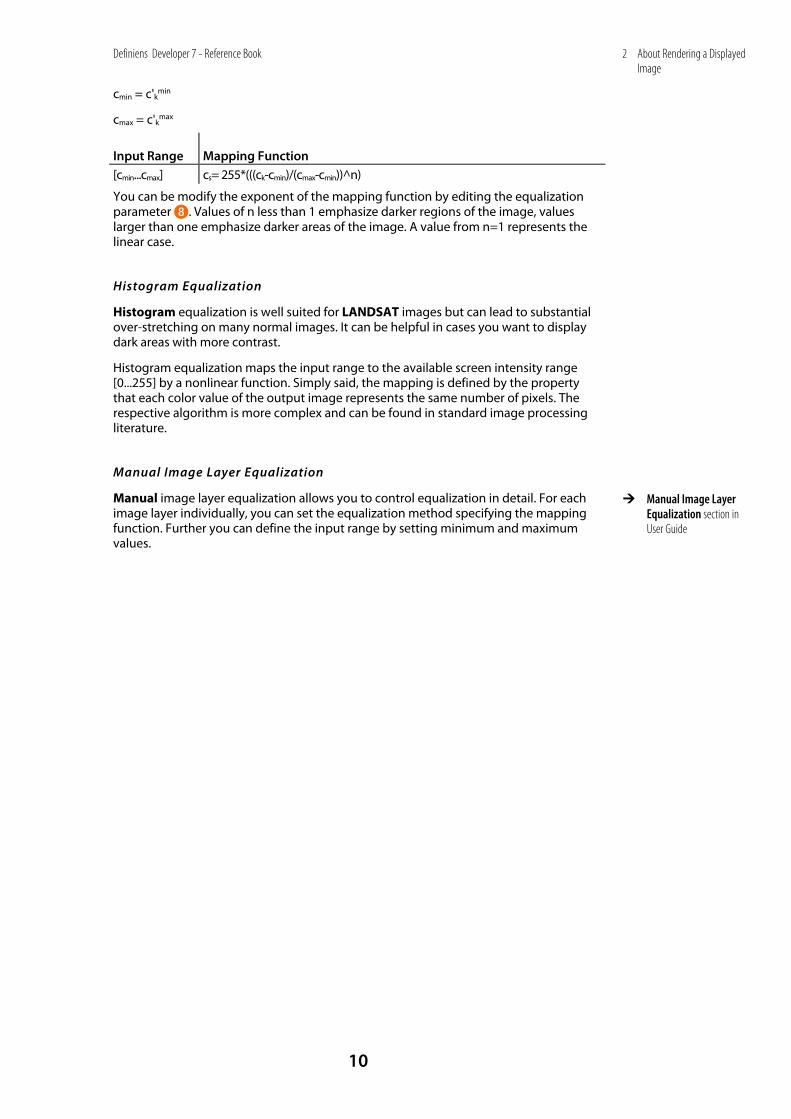
cmin = c'kmin
cmax = c'kmax
Input Range Mapping Function [cmin...cmax] cs= 255*(((ck-cmin)/(cmax-cmin))^n)
You can be modify the exponent of the mapping function by editing the equalization parameter e. Values of n less than 1 emphasize darker regions of the image, values larger than one emphasize darker areas of the image. A value from n=1 represents the linear case.
Histogram Equalization
Histogram equalization is well suited for LANDSAT images but can lead to substantial over-stretching on many normal images. It can be helpful in cases you want to display dark areas with more contrast.
Histogram equalization maps the input range to the available screen intensity range [0...255] by a nonlinear function. Simply said, the mapping is defined by the property that each color value of the output image represents the same number of pixels. The respective algorithm is more complex and can be found in standard image processing literature.
Manual Image Layer Equalization
Manual image layer equalization allows you to control equalization in detail. For each image layer individually, you can set the equalization method specifying the mapping function. Further you can define the input range by setting minimum and maximum values.
Manual Image Layer Equalization section in User Guide
Definiens Developer 7 - Reference Book
11
3 Algorithms Reference
3 Algorithms Reference Contents in This Chapter Process Related Operation Algorithms 13
Segmentation Algorithms 15
Basic Classification Algorithms 28
Advanced Classification Algorithms 29
Variables Operation Algorithms 37
Reshaping Algorithms 40
Level Operation Algorithms 49
Training Operation Algorithms 50
Vectorization Algorithms 54
Sample Operation Algorithms 54
Image Layer Operation Algorithms 56
Thematic Layer Operation Algorithms 66
Export Algorithms 67
Workspace Automation Algorithms 74
Customized Algorithms 81
A single process executes an algorithm on an image object domain. It is the elementary unit of a rule set providing a solution to a specific image analysis problem. Processes are the main working tools for developing rule sets. A rule set is a sequence of processes which are executed in the defined order.
The image object domain is a set of image objects. Every process loops through this set of image objects one by one and applies the algorithm to each single image object. This image object is referred to as the current image object.
Create a Process
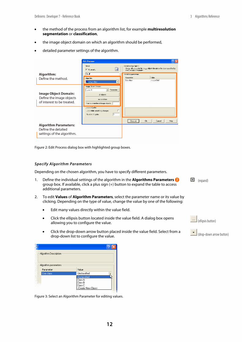
A single process can be created using the Edit Process dialog box in which you can define:
Use Processes section ot the User Guide
Definiens Developer 7 - Reference Book
12
3 Algorithms Reference
• the method of the process from an algorithm list, for example multiresolution segmentation or classification,
• the image object domain on which an algorithm should be performed,
• detailed parameter settings of the algorithm.
Figure 2: Edit Process dialog box with highlighted group boxes.
Specify Algorithm Parameters
Depending on the chosen algorithm, you have to specify different parameters.
1. Define the individual settings of the algorithm in the Algorithms Parameters _ group box. If available, click a plus sign (+) button to expand the table to access additional parameters.
2. To edit Values of Algorithm Parameters, select the parameter name or its value by clicking. Depending on the type of value, change the value by one of the following:
• Edit many values directly within the value field.
• Click the ellipsis button located inside the value field. A dialog box opens allowing you to configure the value.
• Click the drop-down arrow button placed inside the value field. Select from a drop-down list to configure the value.
Figure 3: Select an Algorithm Parameter for editing values.
(expand)
(ellipsis button)
(drop-down arrow button)
Definiens Developer 7 - Reference Book
13
3 Algorithms Reference
3.1 Process Related Operation Algorithms
The Process Related Operation algorithms are used to control other processes.
3.1.1 Execute Child Processes
Execute all child processes of the process.
Use the execute child processes algorithm in conjunction with the no image object domain to structure to your process tree. A process with this settings serves an container for a sequence of functional related processes.
Use the execute child processes algorithm in conjunction with other image object domains (for example, the image object level domain) to loop over a set of image objects. All contained child processes will be applied to the image objects in the image object domain. In this case the child processes usually use one of the following as image object domain: current image object, neighbor object, super object, sub objects.
3.1.2 Set Rule Set Options Select settings that control the rules of behavior of the rule set.
This algorithm enables you to control certain settings for the rule set or for only part of the rule set. For example, you may want to apply particular settings to analyze large objects and change them to analyze small objects. In addition, because the settings are part of the rule set and not on the client, they are preserved when the rule set is run on a server.
execute child processes
Definiens Developer 7 - Reference Book
14
3 Algorithms Reference
Apply to Child Processes Only
Value Description Yes Setting changes apply to child processes of this algorithm only.
No Settings apply globally, persisting after completion of execution..
Distance Calculation
Value Description
Smallest enclosing rectangle
Uses the smallest enclosing rectangle of an image object for distance calculations.
Center of gravity
Uses the center of gravity of an image object for distance calculations.
Default Reset to the default when the rule set is saved.
Keep Current Keep the current setting when the rule set is saved,
Current Resampling Method
Value Description
Center of Pixel Resampling occurs from the center of the pixel.
Upper left corner of pixel
Resampling occurs from the upper left corner of the pixel.
Default Reset to the default when the rule set is saved.
Keep Current Keep the current setting when the rule set is saved.
Evaluate Conditions on Undefined Features as 0
Value Description Yes Ignore undefined features.
No Evaluate undefined features as 0.
Default Reset to the default when the rule set is saved.
Keep Current Keep the current setting when the rule set is saved.
Polygons Base Polygon Threshold
Set the degree of abstraction for the base polygons.
Default: 1.25
Polygons Shape Polygon Threshold
Set the degree of abstraction for the shape polygons. Shape polygons are independent of the topological structure and consist of at least three points. The threshold for shape polygons can be changed any time without the need to recalculate the base vectorization.
Default: 1
Definiens Developer 7 - Reference Book
15
3 Algorithms Reference
Polygons Remove Slivers
Enable Remove slivers to avoid intersection of edges of adjacent polygons and self-intersections of polygons.
Sliver removal becomes necessary with higher threshold values for base polygon generation. Note that the processing time to remove slivers is high, especially for low thresholds where it is not needed anyway.
Value Description
No Allow intersection of polygon edges and self-intersections.
Yes Avoid intersection of edges of adjacent polygons and self-intersections of polygons.
Default Reset to the default when the rule set is saved.
Keep Current Keep the current setting when the rule set is saved.
3.2 Segmentation Algorithms Segmentation algorithms are used to subdivide the entire image represented by the pixel level domain or specific image objects from other domains into smaller image objects.
Definiens provides several different approaches to this well known problem ranging from very simple algorithms like chessboard and quadtree based segmentation to highly sophisticated methods like multiresolution segmentation or the contrast filter segmentation.
Segmentation algorithms are required whenever you want to create new image objects levels based on the image layer information. But they are also a very valuable tool to refine existing image objects by subdividing them into smaller pieces for a more detailed analysis.
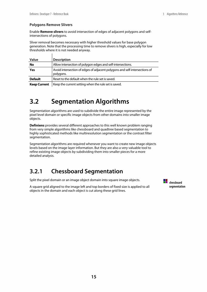
3.2.1 Chessboard Segmentation I
Split the pixel domain or an image object domain into square image objects.
A square grid aligned to the image left and top borders of fixed size is applied to all objects in the domain and each object is cut along these grid lines.
chessboard segmentation
Definiens Developer 7 - Reference Book
16
3 Algorithms Reference
Example
Figure 4: Result of chessboard segmentation with object size 20.
Object Size
The Object size defines the size of the square grid in pixels.
Note
Variables will be rounded to the nearest integer.
Level Name
Enter the name for the new image object level.
Precondition: This parameter is only available, if the domain pixel level is selected in the process dialog.
Thematic Layers
Specify the thematic layers that are to be considered in addition for segmentation.
Each thematic layer that is used for segmentation will lead to additional splitting of image objects while enabling consistent access to its thematic information. You can segment an image using more than one thematic layer. The results are image objects representing proper intersections between the thematic layers.
Precondition: Thematic layers must be available.
If you want to produce image objects based exclusively on thematic layer information, you can select a chessboard size larger than you image size.
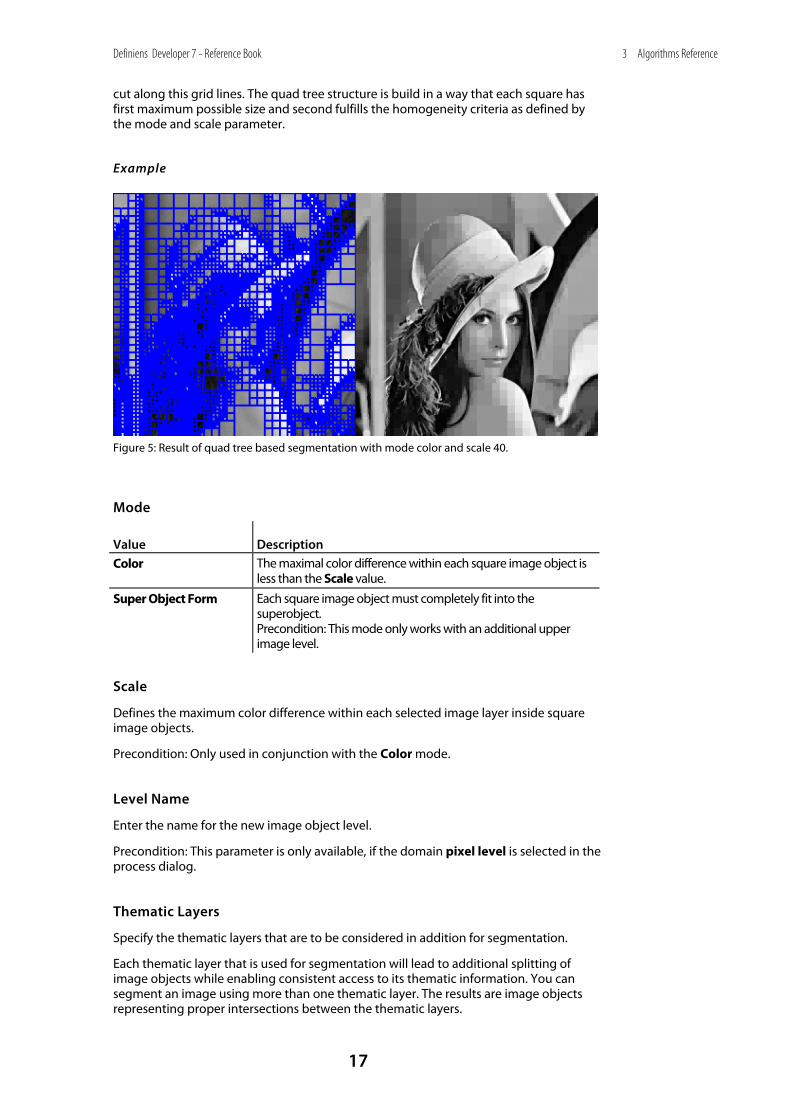
3.2.2 Quad Tree Based Segmentation
Split the pixel domain or an image object domain into a quad tree grid formed by square objects.
A quad tree grid consists of squares with sides each having a power of 2 and aligned to the image left and top borders is applied to all objects in the domain and each object is
quad tree based segmentation
Definiens Developer 7 - Reference Book
17
3 Algorithms Reference
cut along this grid lines. The quad tree structure is build in a way that each square has first maximum possible size and second fulfills the homogeneity criteria as defined by the mode and scale parameter.
Example
Figure 5: Result of quad tree based segmentation with mode color and scale 40.
Mode
Value Description
Color The maximal color difference within each square image object is less than the Scale value.
Super Object Form Each square image object must completely fit into the superobject. Precondition: This mode only works with an additional upper image level.
Scale
Defines the maximum color difference within each selected image layer inside square image objects.
Precondition: Only used in conjunction with the Color mode.
Level Name
Enter the name for the new image object level.
Precondition: This parameter is only available, if the domain pixel level is selected in the process dialog.
Thematic Layers
Specify the thematic layers that are to be considered in addition for segmentation.
Each thematic layer that is used for segmentation will lead to additional splitting of image objects while enabling consistent access to its thematic information. You can segment an image using more than one thematic layer. The results are image objects representing proper intersections between the thematic layers.
Definiens Developer 7 - Reference Book
18
3 Algorithms Reference
Precondition: Thematic layers must be available.
3.2.3 Contrast Split Segmentation Use the contrast split segmentation algorithm to segment an image or an image object into dark and bright regions.
The contrast split algorithm segments an image (or image object) based on a threshold that maximizes the contrast between the resulting bright objects (consisting of pixels with pixel values above threshold) and dark objects (consisting of pixels with pixel values below the threshold).
The algorithm evaluates the optimal threshold separately for each image object in the image object domain. If the pixel level is selected in the image object domain, the algorithm first executes a chessboard segmentation, and then performs the split on each square.
The algorithm achieves the optimization by considering different pixel values as potential thresholds. The test thresholds range from the minimum threshold to the maximum threshold, with intermediate values chosen according to the step size and stepping type parameter. If a test threshold satisfies the minimum dark area and minimum bright area criterion, the contrast between bright and dark objects is evaluated. The test threshold causing the largest contrast is chosen as best threshold and used for splitting.
Chessboard Tile Size
Available only if pixel level is selected in the Image Object Domain. Enter the chessboard tile size.
Default: 1000
Level Name
Select or enter the level that will contain the results of the segmentation. Available only if the pixel level is in the image object domain.
Minimum Threshold
Enter the minimum gray value that will be considered for splitting. The algorithm will calculate the threshold for gray values from the Scan Start value to the Scan Stop value.
Default: 0
Maximum Threshold
Enter the maximum gray value that will be considered for splitting. The algorithm will calculate the threshold for gray values from the Scan Start value to the Scan Stop value.
Default: 255
Step Size
Enter the step size by which the threshold will increase from the Minimum threshold to the Maximum threshold. The value will either be added to the threshold or multiplied by the threshold, according to the selection in the Stepping type field.
contrast split segmentation
Chessboard Segmentation on page 15
Definiens Developer 7 - Reference Book
19
3 Algorithms Reference
The algorithm recalculates a new best threshold each time the threshold is changed by application of the values in the Step size and Stepping type fields, until the Maximum threshold is reached.
Higher values entered for Step size will tend to execute more quickly; smaller values will tend to achieve a split with a larger contrast between bright and dark objects.
Stepping Type
Use the drop-down list to select one of the following:
add: Calculate each step by adding the value in the Scan Step field.
multiply: Calculate each step by multiplying by the value in the Scan Step field.
Image Layer
Select the image layer where the contrast is to be maximized.
Class for Bright Objects
Create a class for image objects brighter than the threshold or select one from the drop-down list. Image objects will not be classified if the value in the Execute splitting field is No.
Class for Dark Objects
Create a class for image objects darker than the threshold or select one from the drop-down list. Image objects will not be classified if the value in the Execute splitting field is No.
Contrast Mode
Select the method the algorithm uses to calculate contrast between bright and dark objects. The algorithm calculates possible borders for image objects and the border values are used in two of the following methods.
a = the mean of bright border pixels.
b = the mean of dark border pixels.
Value Description edge ratio a – b/a + b
edge difference
a – b
object difference
The difference between the mean of all bright pixels and the mean of all dark pixels.
Execute Splitting
Select Yes to split objects with best detected threshold. Select No to simply compute the threshold without splitting.
Best Threshold
Enter a variable to store the computed pixel value threshold that maximizes the contrast.
Definiens Developer 7 - Reference Book
20
3 Algorithms Reference
Best Contrast
Enter a variable to store the computed contrast between bright and dark objects when splitting with the best threshold. The computed value will be different for each Contrast mode.
Minimum Relative Area Dark
Enter the minimum relative dark area.
Segmentation into dark and bright objects only occurs if the relative dark area will be higher than the value entered.
Only thresholds that lead to a relative dark area larger than value entered are considered as best threshold.
Setting this value to a number greater than 0 may increase speed of execution.
Minimum Relative Area Bright
Enter the minimum relative bright area.
Only thresholds that lead to a relative bright area larger than value entered are considered as best threshold.
Setting this value to a number greater than 0 may increase speed of execution.
Minimum Contrast
Enter the minimum contrast value threshold. Segmentation into dark and bright objects only occurs if a contrast higher than the value entered can be achieved.
Minimum Object Size
Enter the minimum object size in pixels that can result from segmentation.
Only larger objects will be segmented. Smaller objects will be merged with neighbors randomly.
The default value of 1 effectively inactivates this option.
Definiens Developer 7 - Reference Book
21
3 Algorithms Reference
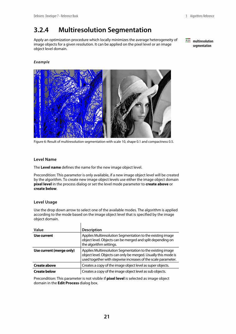
3.2.4 Multiresolution Segmentation
Apply an optimization procedure which locally minimizes the average heterogeneity of image objects for a given resolution. It can be applied on the pixel level or an image object level domain.
Example
Figure 6: Result of multiresolution segmentation with scale 10, shape 0.1 and compactness 0.5.
Level Name
The Level name defines the name for the new image object level.
Precondition: This parameter is only available, if a new image object level will be created by the algorithm. To create new image object levels use either the image object domain pixel level in the process dialog or set the level mode parameter to create above or create below.
Level Usage
Use the drop down arrow to select one of the available modes. The algorithm is applied according to the mode based on the image object level that is specified by the image object domain.
Value Description
Use current Applies Multiresolution Segmentation to the existing image object level. Objects can be merged and split depending on the algorithm settings.
Use current (merge only) Applies Multiresolution Segmentation to the existing image object level. Objects can only be merged. Usually this mode is used together with stepwise increases of the scale parameter.
Create above Creates a copy of the image object level as super objects.
Create below Creates a copy of the image object level as sub objects.
Precondition: This parameter is not visible if pixel level is selected as image object domain in the Edit Process dialog box.
multiresolution segmentation

Definiens Developer 7 - Reference Book
22
3 Algorithms Reference
Image Layer Weights
Image layers can be weighted differently to consider image layers depending on their importance or suitability for the segmentation result.
The higher the weight which is assigned to an image layer, the more of its information will be used during the segmentation process , if it utilizes the pixel information. Consequently, image layers that do not contain the information intended for representation by the image objects should be given little or no weight.
Example: When segmenting a geographical LANDSAT scene using multiresolution segmentation, the segmentation weight for the spatially coarser thermal layer should be set to 0 in order to avoid deterioration of the segmentation result by the blurred transient between image objects of this layer.
Thematic Layers
Specify the thematic layers that are to be considered in addition for segmentation.
Each thematic layer that is used for segmentation will lead to additional splitting of image objects while enabling consistent access to its thematic information. You can segment an image using more than one thematic layer. The results are image objects representing proper intersections between the thematic layers.
Precondition: Thematic layers must be available.
Scale Parameter
The Scale parameter is an abstract term which determines the maximum allowed heterogeneity for the resulting image objects. For heterogeneous data the resulting objects for a given scale parameter will be smaller than in more homogeneous data. By modifying the value in the Scale parameter value you can vary the size of image objects.
Tip
Produce Image Objects that Suit the Purpose (1)
Always produce image objects of the biggest possible scale which still distinguishes different image regions (as large as possible and as fine as necessary). There is a tolerance concerning the scale of the image objects representing an area of a consistent classification due to the equalization achieved by the classification. The separation of different regions is more important than the scale of image objects.

Definiens Developer 7 - Reference Book
23
3 Algorithms Reference
Composition of Homogeneity Criterion
The object homogeneity to which the scale parameter refers is defined in the Composition of homogeneity criterion field. In this circumstance, homogeneity is used as a synonym for minimized heterogeneity. Internally three criteria are computed: Color, smoothness, and compactness. These three criteria for heterogeneity maybe applied multifariously. For most cases the color criterion is the most important for creating meaningful objects. However, a certain degree of shape homogeneity often improves the quality of object extraction. This is due to the fact that the compactness of spatial objects is associated with the concept of image shape. Thus, the shape criteria are especially helpful in avoiding highly fractured image object results in strongly textured data (for example, radar data).
Figure 7: Multiresolution concept flow diagram.
Color and Shape
By modify the shape criterion, you indirectly define the color criteria. In effect, by decreasing the value assigned to the Shape field, you define to which percentage the spectral values of the image layers will contribute to the entire homogeneity criterion. This is weighted against the percentage of the shape homogeneity, which is defined in the Shape field. Changing the weight for the Shape criterion to 1 will result in objects more optimized for spatial homogeneity. However, the shape criterion cannot have a value more than 0.9, due to the obvious fact that without the spectral information of the image, the resulting objects would not be related to the spectral information at all.
Use the slider bar to adjust the amount of Color and Shape to be used for the segmentation.
Note
The color criterion is indirectly defined by the Shape value.
The Shape value can not exceed 0.9.

Definiens Developer 7 - Reference Book
24
3 Algorithms Reference
Tip
Produce Image Objects that Suit the Purpose (2)
Use as much color criterion as possible while keeping the shape criterion as high as necessary to produce image objects of the best border smoothness and compactness. The reason for this is that a high degree of shape criterion works at the cost of spectral homogeneity. However, the spectral information is, at the end, the primary information contained in image data. Using too much shape criterion can therefore reduce the quality of segmentation results.
In addition to spectral information the object homogeneity is optimized with regard to the object shape. The shape criterion is composed of two parameters:
Smoothness
The smoothness criterion is used to optimize image objects with regard to smoothness of borders. To give an example, the smoothness criterion should be used when working on very heterogeneous data to inhibit the objects from having frayed borders, while maintaining the ability to produce non-compact objects.
Compactness
The compactness criterion is used to optimize image objects with regard to compactness. This criterion should be used when different image objects which are rather compact, but are separated from non-compact objects only by a relatively weak spectral contrast.
Use the slider bar to adjust the amount of Compactness and Smoothness to be used for the segmentation.
Note
It is important to notice that the two shape criteria are not antagonistic. This means that an object optimized for compactness might very well have smooth borders. Which criterion to favor depends on the actual task.
3.2.5 Spectral Difference Segmentation
Merge neighboring objects according to their mean layer intensity values. Neighboring image objects are merged if the difference between their layer mean intensities is below the value given by the maximum spectral difference.
This algorithm is designed to refine existing segmentation results, by merging spectrally similar image objects produced by previous segmentations.
Note
This algorithm cannot be used to create new image object levels based on the pixel level domain.
Level Name
The Level name defines the name for the new image object level.
spectral difference segmentation

Definiens Developer 7 - Reference Book
25
3 Algorithms Reference
Precondition: This parameter is only available, if a new image object level will be created by the algorithm. To create new image object levels use either the image object domain pixel level in the process dialog or set the level mode parameter to create above or create below.
Maximum Spectral Difference
Define the amount of spectral difference between the new segmentation for the generated image objects. If the difference is below this value, neighboring objects are merged.
Image Layer Weights
Image layers can be weighted differently to consider image layers depending on their importance or suitability for the segmentation result.
The higher the weight which is assigned to an image layer, the more of its information will be used during the segmentation process , if it utilizes the pixel information. Consequently, image layers that do not contain the information intended for representation by the image objects should be given little or no weight.
Example: When segmenting a geographical LANDSAT scene using multiresolution segmentation, the segmentation weight for the spatially coarser thermal layer should be set to 0 in order to avoid deterioration of the segmentation result by the blurred transient between image objects of this layer.
Thematic Layers
Specify the thematic layers that are to be considered in addition for segmentation.
Each thematic layer that is used for segmentation will lead to additional splitting of image objects while enabling consistent access to its thematic information. You can segment an image using more than one thematic layer. The results are image objects representing proper intersections between the thematic layers.
Precondition: Thematic layers must be available.
3.2.6 Contrast Filter Segmentation
Use pixel filters to detect potential objects by contrast and gradient and create suitable object primitives. An integrated reshaping operation modifies the shape of image objects to help form coherent and compact image objects.
The resulting pixel classification is stored in an internal thematic layer. Each pixel is classified as one of the following classes: no object, object in first layer, object in second layer, object in both layers, ignored by threshold.
Finally a chessboard segmentation is used to convert this thematic layer into an image object level.
Use this algorithm as first step of your analysis to improve overall image analysis performance substantially.
Chessboard Segmentation
The settings configure the final chessboard segmentation of the internal thematic layer.
contrast filter segmentation
Definiens Developer 7 - Reference Book
26
3 Algorithms Reference
See chessboard segmentation reference.
Input Parameters
These parameters are identical for the first and the second layer.
Layer
Choose the image layer to analyze form the drop-down menu. Use <no layer> to disable one of the two filters. If you select <no layer>, then the following parameters will be inactive.
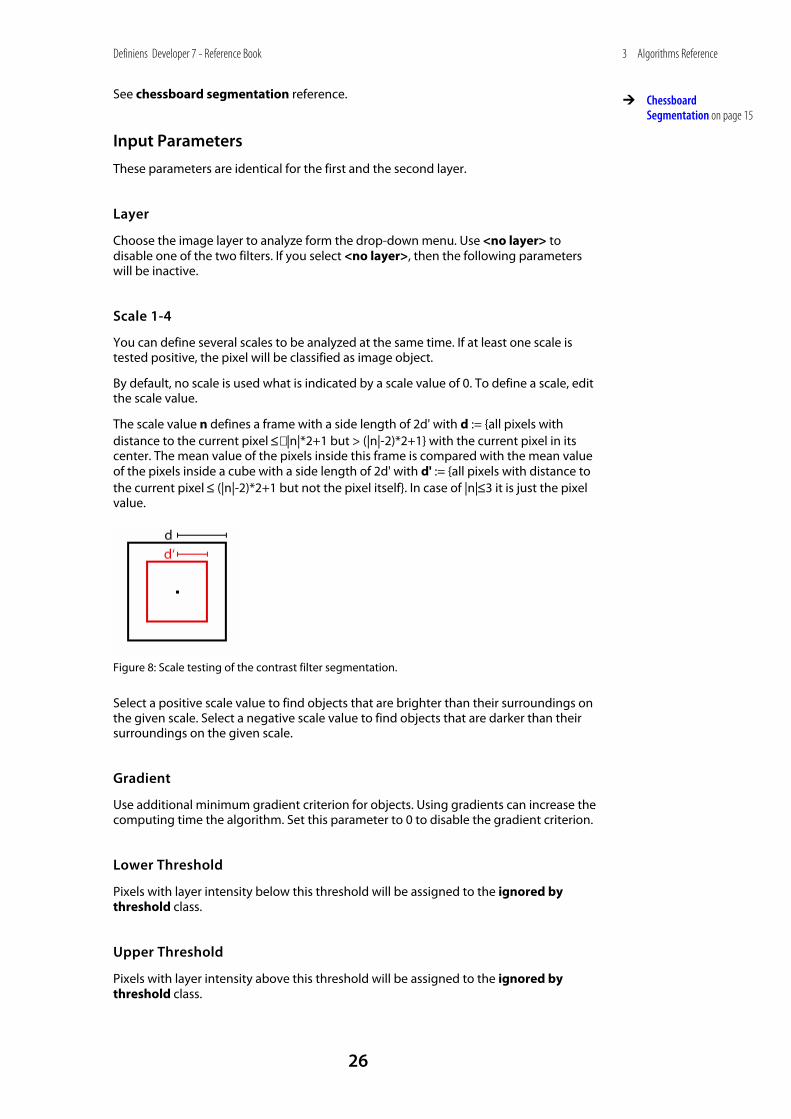
Scale 1-4
You can define several scales to be analyzed at the same time. If at least one scale is tested positive, the pixel will be classified as image object.
By default, no scale is used what is indicated by a scale value of 0. To define a scale, edit the scale value.
The scale value n defines a frame with a side length of 2d' with d := {all pixels with distance to the current pixel ≤ |n|*2+1 but > (|n|-2)*2+1} with the current pixel in its center. The mean value of the pixels inside this frame is compared with the mean value of the pixels inside a cube with a side length of 2d' with d' := {all pixels with distance to the current pixel ≤ (|n|-2)*2+1 but not the pixel itself}. In case of |n|≤3 it is just the pixel value.
Figure 8: Scale testing of the contrast filter segmentation.
Select a positive scale value to find objects that are brighter than their surroundings on the given scale. Select a negative scale value to find objects that are darker than their surroundings on the given scale.
Gradient
Use additional minimum gradient criterion for objects. Using gradients can increase the computing time the algorithm. Set this parameter to 0 to disable the gradient criterion.
Lower Threshold
Pixels with layer intensity below this threshold will be assigned to the ignored by threshold class.
Upper Threshold
Pixels with layer intensity above this threshold will be assigned to the ignored by threshold class.
Chessboard Segmentation on page 15

Definiens Developer 7 - Reference Book
27
3 Algorithms Reference
ShapeCriteria Settings
If you expect coherent and compact image objects, the shape criteria parameter provides an integrated reshaping operation which modifies the shape of image objects by cutting protruding parts and filling indentations and hollows.
ShapeCriteria Value
Protruding parts of image objects are declassified if a direct line crossing the hollow is smaller or equal than the ShapeCriteria value.
Indentations and hollows of image objects are classified as the image object if a direct line crossing the hollow is smaller or equal than the ShapeCriteria value.
If you do not want any reshaping, set the ShapeCriteria value to 0.
Working on Class
Select a class of image objects for reshaping.
Classification Parameters
The pixel classification can be transferred to the image object level using the class parameters.
Classification Parameters
Enable Class Assignment
Select Yes or No in order to use or disable the Classification parameters. If you select No, then the following parameters will be inactive.
No Objects
Pixels failing to meet the defined filter criteria will be assigned the selected class.
Ignored by Threshold
Pixels with layer intensity below or above the Threshold value will be assigned the selected class.
Object in First Layer
Pixels than match the filter criteria in First layer, but not the Second layer will be assigned the selected class.
Objects in Both Layers
Pixels than match the filter criteria value in both Layers will be assigned the selected class.
Objects in Second Layer
Pixels than match the Scale value in Second layer, but not the First layer will be assigned the selected class.
Definiens Developer 7 - Reference Book
28
3 Algorithms Reference
3.3 Basic Classification Algorithms Classification algorithms analyze image objects according defined criteria and assign them each to a class that best meets the defined criteria.
3.3.1 Assign Class
Assign all objects of the image object domain to the class specified by the Use class parameter. The membership value for the assigned class is set to 1 for all objects independent of the class description. The second and third best classification results are set to 0 .
Use class
Select the class for the assignment from the drop-down list box. You can also create a new class for the assignment within the drop-down list.
3.3.2 Classification
Evaluates the membership value of an image object to a list of selected classes. The classification result of the image object is updated according to the class evaluation result. The three best classes are stored in the image object classification result. Classes without a class description are assumed to have a membership value of 1.
Active classes
Choose the list of active classes for the classification.
Erase old classification, if there is no new classification
Value Description Yes If the membership value of the image object is below the acceptance threshold
(see classification settings) for all classes, the current classification of the image object is deleted.
No If the membership value of the image object is below the acceptance threshold (see classification settings) for all classes, the current classification of the image object is kept.
Use Class Description
Value Description Yes Class descriptions are evaluated for all classes. The image object is assigned to the
class with the highest membership value.
No Class descriptions are ignored. This option delivers valuable results only if Active classes contains exactly one class.
If you do not use the class description, it is recommended to use the algorithm assign class algorithm instead.
assign class
classification
Assign Class on page 28

Definiens Developer 7 - Reference Book
29
3 Algorithms Reference
3.3.3 Hierarchical Classification
Evaluate the membership value of an image object to a list of selected classes.
The classification result of the image object is updated according to the class evaluation result. The three best classes are stored as the image object classification result. Classes without a class description are assumed to have a membership value of 0. Class related features are considered only if explicitly enabled by the according parameter.
Note
This algorithm is optimized for applying complex class hierarchies to entire image object levels. This reflects the classification algorithm of eCognition Professional 4. When working with domain specific classification in processes the algorithms assign class and classification are recommended.
Active classes
Choose the list of active classes for the classification.
Use Class-Related Features
Enable to evaluate all class-related features in the class descriptions of the selected classes. If this is disabled these features will be ignored.
3.3.4 Remove Classification
Delete specific classification results from image objects.
Classes
Select classes that should be deleted from image objects.
Process
Enable to delete computed classification results created via processes and other classification procedures from the image object.
Manual
Enable to delete manual classification results from the image object.
3.4 Advanced Classification Algorithms
Advanced classification algorithms classify image objects that fulfill special criteria like being enclosed by another image object or being the smallest or the largest object in a hole set of object.
hierarchical classification
remove classification
Definiens Developer 7 - Reference Book
30
3 Algorithms Reference
3.4.1 Find Domain Extrema
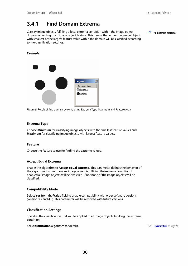
Classify image objects fulfilling a local extrema condition within the image object domain according to an image object feature. This means that either the image object with smallest or the largest feature value within the domain will be classified according to the classification settings.
Example
Figure 9: Result of find domain extrema using Extrema Type Maximum and Feature Area.
Extrema Type
Choose Minimum for classifying image objects with the smallest feature values and Maximum for classifying image objects with largest feature values.
Feature
Choose the feature to use for finding the extreme values.
Accept Equal Extrema
Enable the algorithm to Accept equal extrema. This parameter defines the behavior of the algorithm if more than one image object is fulfilling the extreme condition. If enabled all image objects will be classified. If not none of the image objects will be classified.
Compatibility Mode
Select Yes from the Value field to enable compatibility with older software versions (version 3.5 and 4.0). This parameter will be removed with future versions.
Classification Settings
Specifies the classification that will be applied to all image objects fulfilling the extreme condition.
See classification algorithm for details.
find domain extrema
Classification on page 28

Definiens Developer 7 - Reference Book
31
3 Algorithms Reference
Note
At least one class needs to be selected in the active class list for this algorithm
3.4.2 Find Local Extrema
Classify image objects fulfilling a local extrema condition according to an image object feature within a search domain in their neighborhood. Image objects with either the smallest or the largest feature value within a specific neighborhood will be classified according to the classification settings.
Example
Parameter Value Image Object Domain all objects on level classified as center
Feature Area
Extrema Type Maximum
Search Range 80 pixels
Class Filter for Search center, N1, N2, biggest
Connected A) true B) false
Search Settings
With the Search Settings you can specify a search domain for the neighborhood around the image object.
Class Filter
Choose the classes to be searched. Image objects will be part of the search domain if they are classified with one of the classes selected in the class filter.
Note
Always add the class selected for the classification to the search class filter. Otherwise cascades of incorrect extrema due to the reclassification during the execution of the algorithm may appear.
find local extrema
Definiens Developer 7 - Reference Book
32
3 Algorithms Reference
Search Range
Define the search range in pixels. All image objects with a distance below the given search range will be part of the search domain. Use the drop down arrows to select zero or positive numbers.
Connected
Enable to ensure that all image objects in the search domain are connected with the analyzed image object via other objects in the search range.
Compatibility Mode
Select Yes from the Value field to enable compatibility with older software versions (version 3.5 and 4.0). This parameter will be removed with future versions.
Conditions
Define the extrema conditions.
Extrema Type
Choose Minimum for classifying image objects with the smallest feature values and Maximum for classifying image objects with largest feature values.
Feature
Choose the feature to use for finding the extreme values.
Extrema Condition
This parameter defines the behaviour of the algorithm if more than one image object is fulfilling the extrema condition.
Value Description Do not accept equal extrema None of the image objects will be classified.
Accept equal extrema All of the image objects will be classified.
Accept first equal extrema The first of the image objects will be classified.
Classification Settings
Specifies the classification that will be applied to all image objects fulfilling the extremal condition.
See classification algorithm for details.
Note
At least one class needs to be selected in the active class list for this algorithm.
Classification on page 28
Definiens Developer 7 - Reference Book
33
3 Algorithms Reference
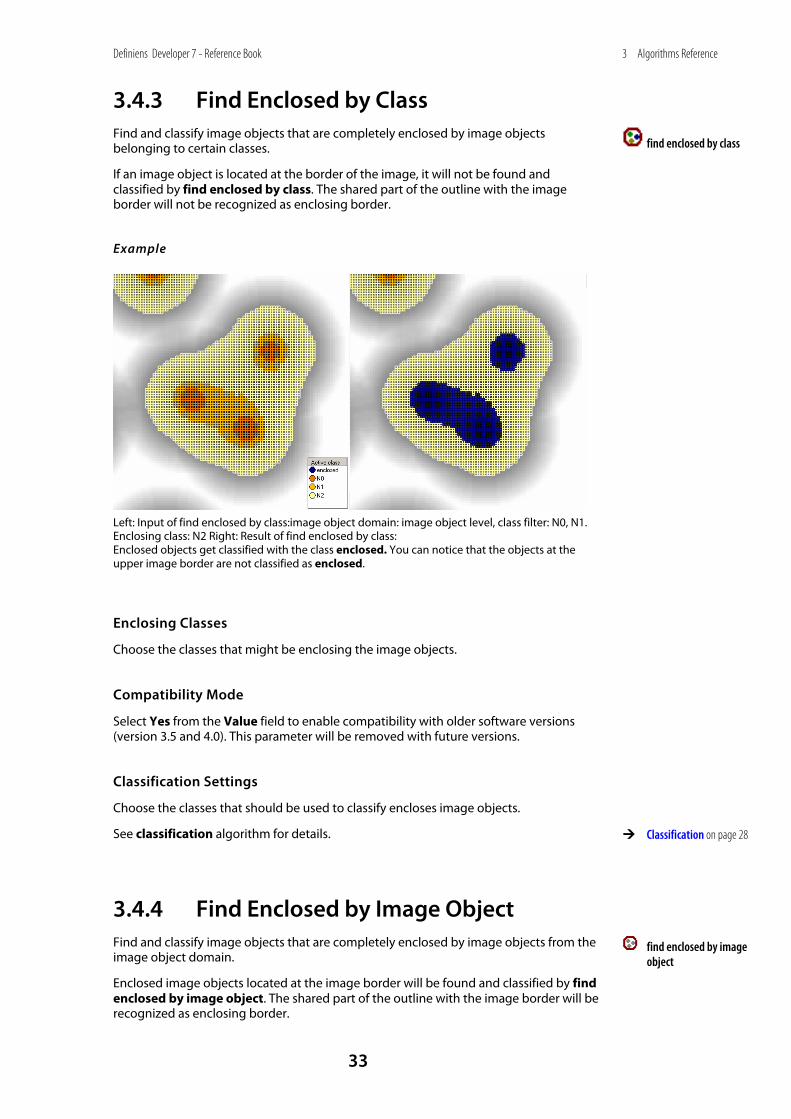
3.4.3 Find Enclosed by Class
Find and classify image objects that are completely enclosed by image objects belonging to certain classes.
If an image object is located at the border of the image, it will not be found and classified by find enclosed by class. The shared part of the outline with the image border will not be recognized as enclosing border.
Example
Left: Input of find enclosed by class:image object domain: image object level, class filter: N0, N1. Enclosing class: N2 Right: Result of find enclosed by class: Enclosed objects get classified with the class enclosed. You can notice that the objects at the upper image border are not classified as enclosed.
Enclosing Classes
Choose the classes that might be enclosing the image objects.
Compatibility Mode
Select Yes from the Value field to enable compatibility with older software versions (version 3.5 and 4.0). This parameter will be removed with future versions.
Classification Settings
Choose the classes that should be used to classify encloses image objects.
See classification algorithm for details.
3.4.4 Find Enclosed by Image Object
Find and classify image objects that are completely enclosed by image objects from the image object domain.
Enclosed image objects located at the image border will be found and classified by find enclosed by image object. The shared part of the outline with the image border will be recognized as enclosing border.
find enclosed by class
Classification on page 28
find enclosed by image object

Definiens Developer 7 - Reference Book
34
3 Algorithms Reference
Example
Left: Input of find enclosed by image object:image object domain: image object level, class filter: N2. Right: Result of find enclosed by image object:enclosed objects are classified with the class enclosed. Note that the objects at the upper image border are classified as enclosed.
Classification Settings
Choose the class that will be used to classify enclosed image objects.
See classification algorithm for details.
3.4.5 Connector
Classify the image objects which connect the current image object with the shortest path to another image object that meets the conditions described by the connection settings.
The process starts from the current image object to search along objects that meet the conditions as specified by Connect via and Super object mode via until it reaches image objects that meet the conditions specified by Connect to and Super object mode to. The maximum search range can be specified in Search range in pixels. When the algorithm has found the nearest image object that can be connected to it classifies all image objects of the connection with the selected class.
Connector Via
Choose the classes you wish to be connected.
Super Object Mode Via
Limit the shorted path use for Super object mode via using one of the following:
Classification on page 28
connector
Definiens Developer 7 - Reference Book
35
3 Algorithms Reference
Value Description
Don't Care Use any image object.
Different Super Object Use only images with a different superobject than the Seed object.
Same Super Object Use only image objects with the same superobject as the Seed object
Connect To
Choose the classes you wish to be connected.
Super Object Mode To
Limit the shorted path use for Super Object Mode To using one of the following:
Value Description
Don't Care Use any image object.
Different Super Object Use only images with a different superobject than the Seed object.
Same Super Object Use only image objects with the same superobject as the Seed object
Search Range
Enter the Search Range in pixels that you wish to search.
Classification Settings
Choose the class that should be used to classify the connecting objects.
See classification algorithm for details.
3.4.6 Optimal Box Generate member functions for classes by looking for the best separating features based upon sample training.
Sample Class
For target samples
Class that provides samples for target class (class to be trained). Select a class or create a new class.
For rest samples
Class that provides samples for the rest of the domain.
Select a class or create a new class.
Classification on page 28
optimal box
Definiens Developer 7 - Reference Book
36
3 Algorithms Reference
Insert Membership Function
For target samples into
Class that receives membership functions after optimization for target. If set to unclassified, the target sample class is used.
Select a class or create a new class.
For rest samples into
Class that receives inverted similarity membership functions after optimization for target. If set to unclassified, the rest sample class is used.
Select a class or create a new class.
Clear all membership functions
When inserting new membership functions into the active class, choose whether to clear all existing membership functions or clear only those from input feature space.
Value Description
No, only clear if associated with input feature space
Clear membership functions only from the input feature space when inserting new membership functions into the active class.
Yes, always clear all membership functions
Clear all membership functions when inserting new membership functions into the active class.
Border membership value
Border y-axis value if no rest sample exists in that feature direction.
Default: 0.66666
Feature Optimization
Input Feature Set
Input set of descriptors from which a subset will be chosen.
Click the ellipsis button to open the Select Multiple Features dialog box and select features by double-clicking in the Available pane to move features to the Selected pane. The Ensure selected features are in Standard Nearest Neighbor feature space checkbox is selected by default.
Minimum number of features
Minimum number of features descriptors to employ in class.
Default: 1
Maximum number of features
Maximum number of features descriptors to employ in class.
(ellipsis button)
Definiens Developer 7 - Reference Book
37
3 Algorithms Reference
Optimization Settings
Weighted distance exponent
0: All distances weighted equally.
X: Decrease weighting with increasing distance.
Enter a number greater than 0 to decrease weighting with increasing distance.
Default: 2
Optimization Settings
False positives variable
Variable to be set to the number of false positives after execution.
Enter a variable or select one that has already been created. If you enter a new variable, the Create Variable dialog will open.
False negatives variable
Variable to be set to the number of false positives after execution.
Enter a variable or select one that has already been created. If you enter a new variable, the Create Variable dialog will open.
Show info in message console
Show information on feature evaluations in message console.
3.5 Variables Operation Algorithms Variable operation algorithms are used to modify the values of variables. They provide different methods to perform computations based on existing variables and image object features and store the result within a variable.
3.5.1 Update Variable
Perform an arithmetic operation on a process variable.
Variable Type
Select Object, Scene, Feature, Class, or Level.
Variable
Select an existing variable or enter a new name to add a new one. If you have not already created a variable, the Create variable type Variable dialog box will open.
User Guide chapters: Use Variables in Rule Sets and Create a Variable
Update Variable Algorithm

Definiens Developer 7 - Reference Book
38
3 Algorithms Reference
Feature/Class/Level
Select the variable assignment, according to the variable type selected in the Variable Type field. This field does not display for Object and Scene variables.
To select a variable assignment, click in the field and do one of the following depending on the variable type:
• For feature variables, use the ellipsis button to open the Select Single Feature dialog box and select a feature or create a new feature variable.
• For class variables, use the drop-down arrow to select from existing classes or create a new class.
• For level variables, use the drop-arrow to select from existing levels.
• For object variables, use the drop-arrow to select from existing levels.
Operation
This field displays only for Object and Scene variables.
Select one of the following arithmetic operations:
Value Description
= Assign a value.
+= Increment by value.
−= Decrement by value.
*= Multiply by value.
/= Divide by value.
Assignment
This field displays only for Scene and Object variables.
You can assign either by value or by feature. This setting enables or disables the remaining parameters.
Value
This field displays only for Scene and Object variables.
If you have selected to assign by value, you may enter either a value or a variable. To enter text use quotes. The numeric value of the field or the selected variable will be used for the update operation.
Feature
This field displays only for Scene and Object variables.
If you have chosen to assign by feature you can select a single feature. The feature value of the current image object will be used for the update operation.
Comparison Unit
This field displays only for Scene and Object variables.
If you have chosen to assign by feature, and the selected feature has units, then you may select the unit used by the process. If the feature has coordinates, select
(ellipsis button)
Select Single Feature
(drop-down arrow button)
Definiens Developer 7 - Reference Book
39
3 Algorithms Reference
Coordinates to provide the position of the object within the original image or Pixels to provide the position of the object within the currently used scene.
3.5.2 Compute Statistical Value
Perform a statistical operation on the feature distribution within an image object domain and stores the result in a process variable.
Variable
Select an existing variable or enter a new name to add a new one. If you have not already created a variable, the Create Variable dialog box will open.
Operation
Select one of the following statistical operations:
Value Description Number Count the objects of the currently selected image object domain.
Sum Return the sum of the feature values from all objects of the selected image object domain.
Maximum Return the maximum feature value from all objects of the selected image object domain.
Minimum Return the minimum feature value from all objects of the selected image object domain.
Mean Return the mean feature value of all objects from the selected image object domain.
Standard Deviation Return the standard deviation of the feature value from all objects of the selected image object domain.
Median Return the median feature value from all objects of the selected image object domain.
Quantile Return the feature value, where a specified percentage of objects from the selected image object domain have a smaller feature value.
Parameter
If you have selected the quantile operation specify the percentage threshold [0;100].
Feature
Select the feature that is used to perform the statistical operation.
Precondition: This parameter is not used if you select number as your operation.
Unit
If you have selected a feature related operation, and the feature selected supports units, then you may select the unit for the operation.
compute statistical value
Definiens Developer 7 - Reference Book
40
3 Algorithms Reference
3.5.3 Apply Parameter Set
Writes the values stored inside a parameter set to into the related variables. For each parameter in the parameter set the algorithm scans for a variable with the same name. If this variable exists, then the value of the variable is updated by the value specified in the parameter set.
Precondition: You must first create at least one parameter set.
Parameter Set Name
Select the name of a parameter set.
3.5.4 Update Parameter Set
Writes the values of variable into a parameter set. For each parameter in the parameter set the algorithm scans for a variable with the same name. If this variable exists, then the value of the variable is written to the parameter set.
Precondition: You must first create at least one parameter set.
Parameter Set Name
Select the name of a parameter set.
Tip
Create Parameters
Parameters are created with the Manage Parameter Sets dialog box, which is available on the menu bar under Process or on the tool bar.
3.6 Reshaping Algorithms Reshaping algorithms modify the shape of existing image objects. They execute operations like merging image objects, splitting them into their subobjects and also sophisticated algorithm supporting a variety of complex object shape transformations.
3.6.1 Remove Objects
Merge image objects in the image object domain. Each image object is merged into the neighbor image object with the largest common border.
This algorithm is especially helpful for clutter removal.
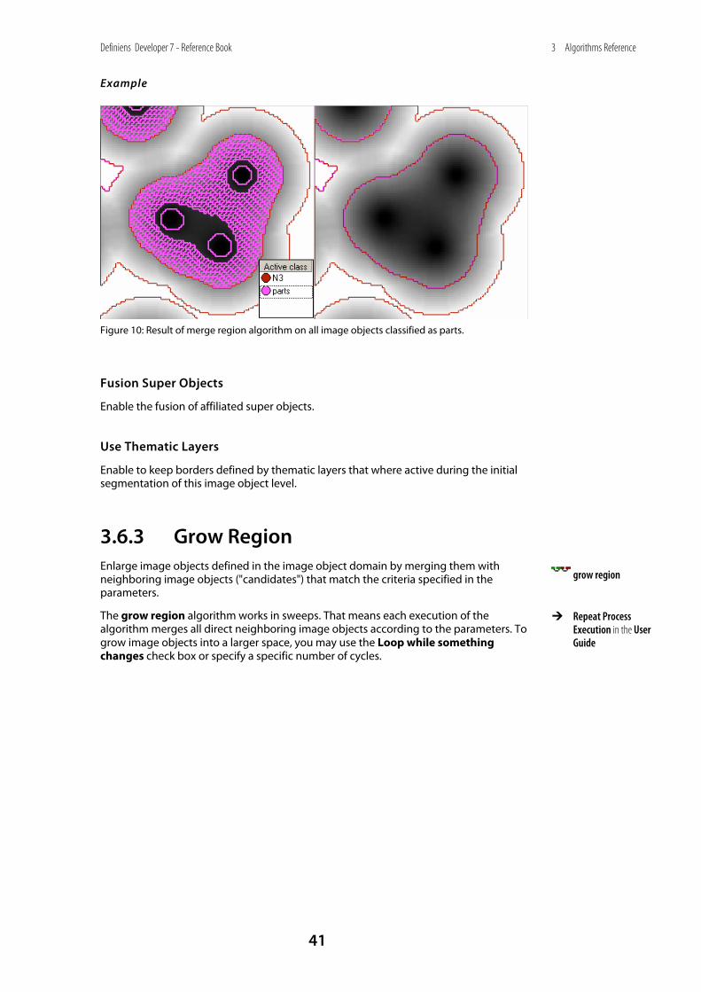
3.6.2 Merge Region
Merge all image objects chosen in the image object domain.
apply parameter set User Guide:
About Parameter Sets
update parameter set User Guide:
About Parameter Sets
remove objects
merge region
Definiens Developer 7 - Reference Book
41
3 Algorithms Reference
Example
Figure 10: Result of merge region algorithm on all image objects classified as parts.
Fusion Super Objects
Enable the fusion of affiliated super objects.
Use Thematic Layers
Enable to keep borders defined by thematic layers that where active during the initial segmentation of this image object level.
3.6.3 Grow Region
Enlarge image objects defined in the image object domain by merging them with neighboring image objects ("candidates") that match the criteria specified in the parameters.
The grow region algorithm works in sweeps. That means each execution of the algorithm merges all direct neighboring image objects according to the parameters. To grow image objects into a larger space, you may use the Loop while something changes check box or specify a specific number of cycles.
grow region
Repeat Process Execution in the User Guide
Definiens Developer 7 - Reference Book
42
3 Algorithms Reference
Example
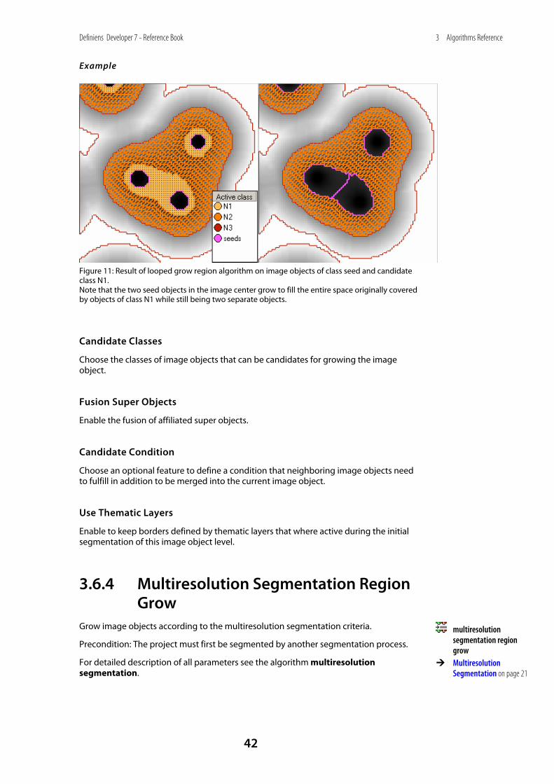
Figure 11: Result of looped grow region algorithm on image objects of class seed and candidate class N1. Note that the two seed objects in the image center grow to fill the entire space originally covered by objects of class N1 while still being two separate objects.
Candidate Classes
Choose the classes of image objects that can be candidates for growing the image object.
Fusion Super Objects
Enable the fusion of affiliated super objects.
Candidate Condition
Choose an optional feature to define a condition that neighboring image objects need to fulfill in addition to be merged into the current image object.
Use Thematic Layers
Enable to keep borders defined by thematic layers that where active during the initial segmentation of this image object level.
3.6.4 Multiresolution Segmentation Region Grow
Grow image objects according to the multiresolution segmentation criteria.
Precondition: The project must first be segmented by another segmentation process.
For detailed description of all parameters see the algorithm multiresolution segmentation.
multiresolution segmentation region grow
Multiresolution Segmentation on page 21
Definiens Developer 7 - Reference Book
43
3 Algorithms Reference
3.6.5 Image Object Fusion
Define a variety of growing and merging methods and specify in detail the conditions for merger of the current image object with neighboring objects.
Tip
If you do not need a fitting functions, we recommend that you use the algorithms merge region and grow regions. They require fewer parameters for configuration and provide higher performance.
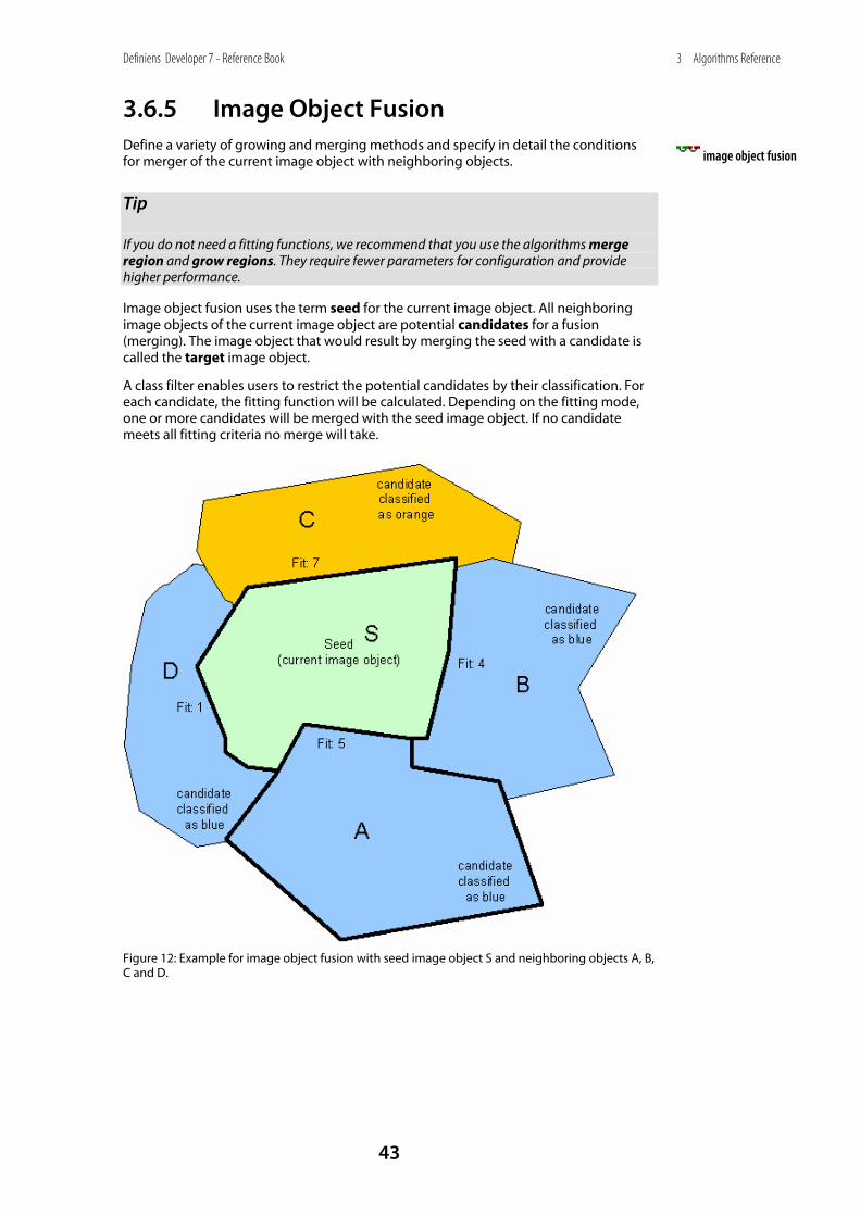
Image object fusion uses the term seed for the current image object. All neighboring image objects of the current image object are potential candidates for a fusion (merging). The image object that would result by merging the seed with a candidate is called the target image object.
A class filter enables users to restrict the potential candidates by their classification. For each candidate, the fitting function will be calculated. Depending on the fitting mode, one or more candidates will be merged with the seed image object. If no candidate meets all fitting criteria no merge will take.
Figure 12: Example for image object fusion with seed image object S and neighboring objects A, B, C and D.
image object fusion
Definiens Developer 7 - Reference Book
44
3 Algorithms Reference
Candidate Settings
Enable Candidate Classes
Select Yes to activate candidate classes. If the candidate classes are disabled the algorithm will behave like a region merging.
Candidate Classes
Choose the candidate classes you wish to consider.
If the candidate classes are distinct from the classes in the image object domain (representing the seed classes), the algorithm will behave like a region growing.
Fitting Function
The fusion settings specify the detailed behavior of the image object fusion algorithm.
Fitting Mode
Choose the fitting mode.
Value Description
all fitting Merges all candidates that match the fitting criteria with the seed.
first fitting Merges the first candidate that matches the fitting criteria with the seed.
best fitting Merges the candidate that matches the fitting criteria in the best way with the seed.
all best fitting Merges all candidates that match the fitting criteria in the best way with the seed.
best fitting if mutual Merges the best candidate if it is calculated as the best for both of the two image objects (seed and candidate) of a combination.
mutual best fitting Executes a mutual best fitting search starting from the seed. The two image objects fitting best for both will be merged. Note: These image objects that are finally merged may not be the seed and one of the original candidate but other image objects with an even better fitting.
Fitting Function Threshold
Select the feature and the condition you want to optimize. The closer a seed candidate pair matches the condition the better the fitting.
Use Absolute Fitting Value
Enable to ignore the sign of the fitting values. All fitting values are treated as positive numbers independent of their sign.
Weighted Sum
Define the fitting function. The fitting function is computed as the weighted sum of feature values. The feature selected in the Fitting function threshold will be calculated
Definiens Developer 7 - Reference Book
45
3 Algorithms Reference
for the seed, candidate, and the target image object. The total fitting value will be computed by the formula
Fitting Value = (Target * Weight) + (Seed * Weight) + (Candidate * Weight)
To disable the feature calculation for any of the three objects, set the according weight to 0
Target Value Factor
Set the weight applied to the target in the fitting function.
Seed Value Factor
Set the weight applied to the seed in the fitting function.
Candidate Value Factor
Set the weight applied to the candidate in the fitting function.
Typical Settings (TVF, SVF, CVF)
Description
1,0,0 Optimize condition on the image object resulting from the merge.
0,1,0 Optimize condition on the seed image object.
0,0,1 Optimize condition on the candidate image object.
2,-1,-1 Optimize the change of the feature by the merge.
Merge Settings
Fusion Super Objects
This parameter defines the behaviour if the seed and the candidate objects that are selected for merging have different super objects. If enabled the super objects will be merged with the sub objects. If disabled the merge will be skipped.
Thematic Layers
Specify the thematic layers that are to be considered in addition for segmentation.
Each thematic layer that is used for segmentation will lead to additional splitting of image objects while enabling consistent access to its thematic information. You can segment an image using more than one thematic layer. The results are image objects representing proper intersections between the thematic layers.
Precondition: Thematic layers must be available.
Compatibility Mode
Select Yes from the Value field to enable compatibility with older software versions (version 3.5 and 4.0). This parameter will be removed with future versions.
Classification Settings
Define a classification to be applied to the merged image objects.
Definiens Developer 7 - Reference Book
46
3 Algorithms Reference
See classification algorithm for details.
3.6.6 Convert to Subobjects
Split all image objects of the image object domain into their subobjects.
Precondition: The image objects in the domain need to have subobjects.
3.6.7 Border Optimization
Change the image object shape by either adding subobjects from the outer border to the image object or removing subobjects from the inner border from the image object.
Candidate Classes
Choose the classes you wish to consider for the subobjects. Subobjects need to be classified with one of the selected classes to be considered by the border optimization.
Destination
Choose the classes you wish to consider for the neighboring objects of the current image object. To be considered by the Dilatation, subobjects need to be part of an image object classified with one of the selected classes. To be considered by the Erosion subobjects need to be moveable to an image object classified with one of the selected classes. This parameter has no effect for the Extraction.
Operation
Value Description
Dilatation Removes all Candidate subobjects from its Destination superobject inner border and merges them to the neighboring image objects of the current image object.
Erosion Removes all Candidate objects from its Seed superobject inner border and merges them to the neighboring image objects of Destination domain.
Extraction Splits an image object by removing all subobjects of the Candidate domain from the image objects of Seed domain.
Classification Settings
The resulting image objects can be classified.
See classification algorithm for details.
Classification on page 28
convert to subobjects
border optimization
Classification on page 28
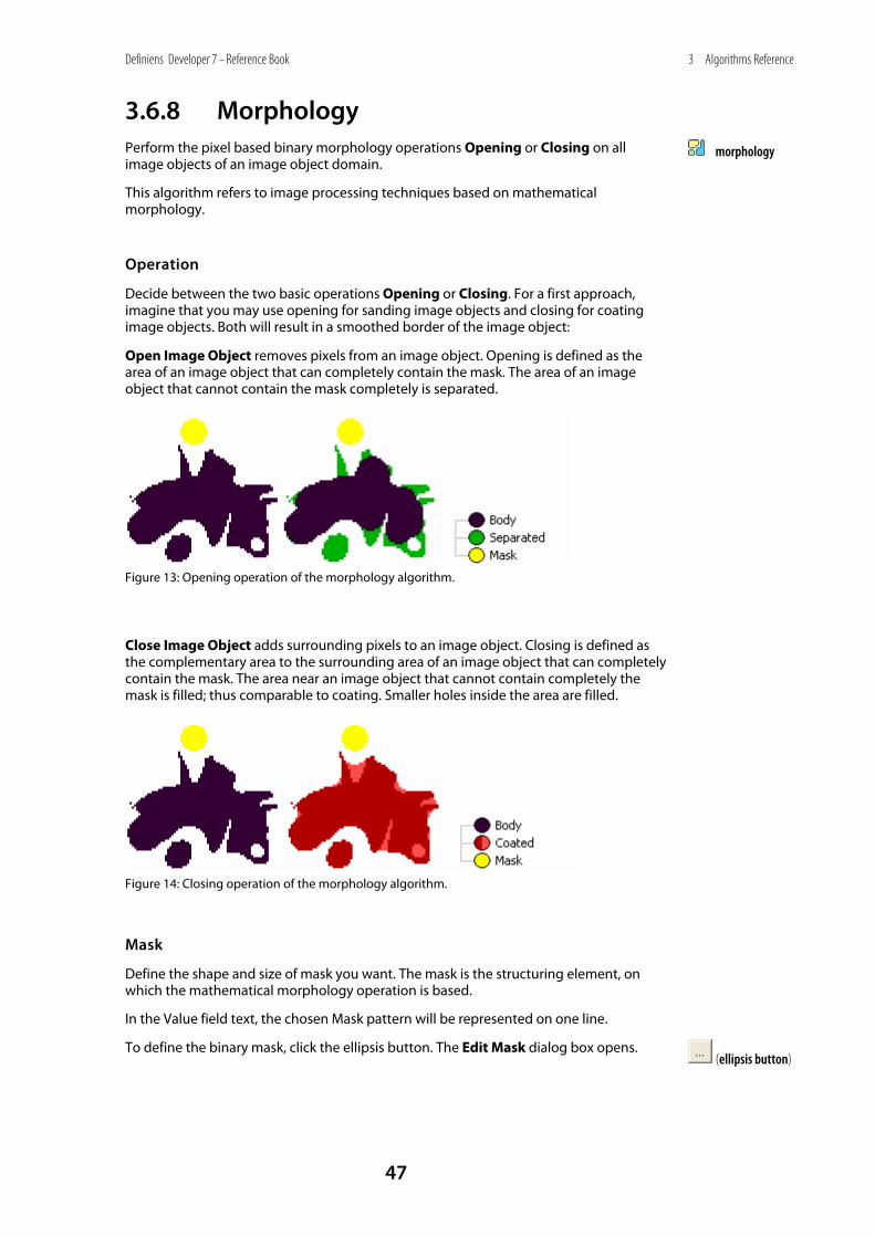
Definiens Developer 7 - Reference Book
47
3 Algorithms Reference
3.6.8 Morphology
Perform the pixel based binary morphology operations Opening or Closing on all image objects of an image object domain.
This algorithm refers to image processing techniques based on mathematical morphology.
Operation
Decide between the two basic operations Opening or Closing. For a first approach, imagine that you may use opening for sanding image objects and closing for coating image objects. Both will result in a smoothed border of the image object:
Open Image Object removes pixels from an image object. Opening is defined as the area of an image object that can completely contain the mask. The area of an image object that cannot contain the mask completely is separated.
Figure 13: Opening operation of the morphology algorithm.
Close Image Object adds surrounding pixels to an image object. Closing is defined as the complementary area to the surrounding area of an image object that can completely contain the mask. The area near an image object that cannot contain completely the mask is filled; thus comparable to coating. Smaller holes inside the area are filled.
Figure 14: Closing operation of the morphology algorithm.
Mask
Define the shape and size of mask you want. The mask is the structuring element, on which the mathematical morphology operation is based.
In the Value field text, the chosen Mask pattern will be represented on one line.
To define the binary mask, click the ellipsis button. The Edit Mask dialog box opens.
morphology
(ellipsis button)
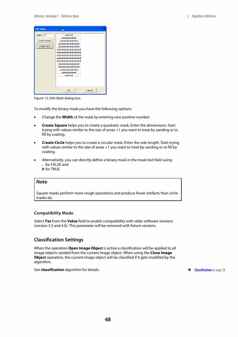
Definiens Developer 7 - Reference Book
48
3 Algorithms Reference
Figure 15: Edit Mark dialog box.
To modify the binary mask you have the following options:
• Change the Width of the mask by entering new positive number.
• Create Square helps you to create a quadratic mask. Enter the dimensions. Start trying with values similar to the size of areas +1 you want to treat by sanding or to fill by coating.
• Create Circle helps you to create a circular mask. Enter the side length. Start trying with values similar to the size of areas +1 you want to treat by sanding or to fill by coating.
• Alternatively, you can directly define a binary mask in the mask text field using . for FALSE and # for TRUE.
Note
Square masks perform more rough operations and produce fewer artifacts than circle masks do.
Compatibility Mode
Select Yes from the Value field to enable compatibility with older software versions (version 3.5 and 4.0). This parameter will be removed with future versions.
Classification Settings
When the operation Open Image Object is active a classification will be applied to all image objects sanded from the current image object. When using the Close Image Object operation, the current image object will be classified if it gets modified by the algorithm.
See classification algorithm for details.
Classification on page 28
Definiens Developer 7 - Reference Book
49
3 Algorithms Reference
3.6.9 Watershed Transformation
The watershed transformation algorithm calculates an inverted distance map based on the inverted distances for each pixel to the image object border. Afterwards, the minima are flooded by increasing the level (inverted distance). Where the individual catchment basins touch each other (watersheds), the image objects are split.
Example of purpose: The Watershed Transformation algorithm is used to separate image objects from others.
Precondition: Image objects that you wish to split should already be identified and classified.
Length Factor
The Length factor is the maximal length of a plateau, which is merged into a catchment basin. Use the toggle arrows in the Value field to change to maximal length.
Note
The Length Factor must be greater or equal to zero.
Classification Settings
Define a classification to be applied if an image object is cut by the algorithm.
See classification algorithm for details.
3.7 Level Operation Algorithms Level operation algorithms allow you to add, remove or rename2 entire image object levels within the image object hierarchy.
3.7.1 Copy Image Object Level
Insert a copy of the selected image objects domain above or below the existing one.
Level Name
Enter the name for the new image object level.
Copy Level
Level copy maybe placed above or below the input level specified by the domain.
watershed transformation
Classification on page 28
copy image object level
Definiens Developer 7 - Reference Book
50
3 Algorithms Reference
3.7.2 Delete Image Object Level
Delete the image object level selected in the image object domain.
3.7.3 Rename Image Object Level
Rename an image object level.
Level to Rename
Select the image object level to be renamed.
New Level Name
Select or edit an image object level to be changed, and select or edit the new name for the level.
If the new name is already assigned to an existing level, that level will be deleted.
This algorithm does not change names already existing in the process tree.
3.8 Training Operation Algorithms Interactive operation algorithms are used for user interaction with the user of actions in Definiens Architect.
3.8.1 Show User Warning
Edit and display a user warning.
Message
Edit the text of the user warning.
3.8.2 Create/Modify Project
Create a new project or modify an existing one.
Image File
Browse for an image file containing the image layers. Alternatively, you can edit the path.
Image Layer ID
Change the image layer ID within the file. Note, that the ID is zero-based.
delete image object level
rename image object level
show user warning
create/modify project User Guide:
Create a New Project
Definiens Developer 7 - Reference Book
51
3 Algorithms Reference
Image Layer Alias
Edit the image layer alias.
Thematic File
Browse for a thematic file containing the thematic layers. Alternatively, you can edit the path.
Attribute Table File
Browse for an attribute file containing thematic layer attributes. Alternatively, you can edit the path.
Attribute ID Column Name
Edit the name of the column of the attribute table containing the thematic layer attributes of interest.
Thematic Layer Alias
Edit the thematic layer alias.
Show Subset Selection
Opens the Subset Selection dialog box when executed interactively.
Enable Geocoding
Activate to select the bounding coordinates based on the respective geographical coordinate system.
3.8.3 Update Action from Parameter Set
Synchronize the values of an action according to the values of a parameter set.
Parameter Set Name
Select the name of a parameter set.
Action Name
Type the name of an action.
update action from parameter set
Definiens Developer 7 - Reference Book
52
3 Algorithms Reference
3.8.4 Update Parameter Set from Action
Synchronize the values of a parameter set according to the values of an action.
Action Name
Type the name of an action.
Parameter Set Name
Select the name of a parameter set.
3.8.5 Manual Classification
Enable the user of an action to classify image objects of the selected class manually by clicking.
Class
Select a class that can be assigned manually.
3.8.6 Configure Object Table
Display a list of all image objects together with selected feature values in the Image Object Table window .
Classes
Select classes to list all of its image objects.
Features
Select the features to display the feature values of the image objects.
3.8.7 Display Image Object Level
Display a selected image object level.
Level Name
Select the image object level to be displayed.
update parameter set from action
manual classification User Guide:
Classify Image Objects Manually
configure object table User Guide:
Compare Multiple Image Objects by Using the Image Object Table
display image object level
User Guide: Navigate Within the Image Object Hierarchy
Definiens Developer 7 - Reference Book
53
3 Algorithms Reference
3.8.8 Select Input Mode
Set the mode for user input via graphical user interface.
Input Mode
Select an input mode:
Value Description Normal Return to normal input mode, for example, selection of image objects
by clicking them.
Manual object cut Activate the Cut Objects Manually function.
3.8.9 Activate Draw Polygons Use the activate draw polygons algorithm to activate thematic editing, creates thematic layer and enable the cursor for drawing. It is designed to be used with actions.
Layer Name
Select the name of the image layer where the polygons will be enabled.
Cursor Actions Available After Execution
• Click and hold the left mouse button as you drag the cursor across the image to create a path with points in the image.
• To create points at closer intervals, drag the cursor more slowly to create points at closer intervals or hold the control key while dragging.
• Release the mouse button to automatically close the polygon.
• Click along a path in the image to create points at each click. To close the polygon, double-click or select Close Polygon in the context menu.
• To delete the last point before the polygon is complete, select Delete Last Point in the context menu.
3.8.10 Select Thematic Objects Use the select thematic objects algorithm to enable selection of thematic objects in the user interface. The algorithm activates thematic editing and enables cursor selection mode. It is designed to be used with actions.
Layer Name
Enter the name of the layer where thematic objects are to be selected.
Selection Mode
Choose the type of selection:
select input mode
activate draw polygons
select thematic objects
Definiens Developer 7 - Reference Book
54
3 Algorithms Reference
• Single: enables selection of single polygons.
• Polygon: enables selection of all shapes within a user-drawn polygon.
• Line: enables selection of all shapes crossed by a user-drawn line.
• Rectangle: enables selection of all shapes within a user-drawn rectangle.
Cursor Actions After Execution
Depending on the Selection Mode, you can select polygons in the following ways. Selected polygons will be outlined in red. After making a selection, delete any selected polygons using the context menu or press Del on the keyboard.
• Single: Click on a polygon to select it.
• Polygon: Left-click and drag around polygons. When the polygon is closed, any enclosed polygons will be selected.
• Line: Left-click and drag in a line across polygons.
• Rectangle: Draw a rectangle around polygons to select them.
3.8.11 End Thematic Edit Mode Use the end thematic edit mode algorithm to switch back from thematic editing to image object editing and save the shape file. It is designed to be used with actions.
Shapes File
Enter the name of the shape file.
3.9 Vectorization Algorithms
Tip
Vectorization algorithms available in earlier versions have been removed because polygons are available automatically for any segmented image. You can use the algorithm parameters in the set rule set options algorithm to change the way polygons are formed.
Set Rule Set Options on page 13
3.10 Sample Operation Algorithms Use sample operation algorithms to perform sample operations.
3.10.1 Classified Image Objects to Samples
Create a sample for each classified image object in the image object domain.
end thematic edit mode
classified image objects to samples

Definiens Developer 7 - Reference Book
55
3 Algorithms Reference
3.10.2 Cleanup Redundant Samples
Remove all samples with membership values higher than the membership threshold.
Membership Threshold
You can modify the default value which is 0.9.
Note
This algorithm might produce different results each time it will be executed. This is because the order of sample deletion is random.
3.10.3 Nearest Neighbor Configuration
Select classes, features and function slope to use for nearest neighbor classification.
Active classes
Choose the classes you wish to use for nearest neighbor classification.
NN Feature Space
Select as many features as you like for the nearest neighbor feature space.
Function Slope
Enter the function slope for the nearest neighbor.
3.10.4 Delete All Samples
Delete all samples.
3.10.5 Delete Samples of Class
Delete all samples of certain classes.
Class List
Select the classes for which samples are to be deleted.
3.10.6 Disconnect All Samples Disconnect samples from image objects, to enable creation of samples that are not lost when image objects are deleted. They are stored in the solution file.
This algorithm has no parameters.
cleanup redundant samples
nearest neighbor configuration
delete all samples
delete samples of class
• disconnect all samples

Definiens Developer 7 - Reference Book
56
3 Algorithms Reference
3.10.7 Sample Selection Use the sample selection algorithm to switch the curser to sample selection mode using the selected class.
Class
Choose a class to use in selecting samples.
3.11 Image Layer Operation Algorithms Image layer operation algorithms are used to create or to delete image object layers. Further you can use the image layer operation algorithms to apply filters to image layers at the pixel level.
3.11.1 Create Temporary Image Layer
Create a temporary image layer with values calculated from a selected feature for the image objects selected in the image object domain.
Layer Name
Select the default name for the temporary image layer or edit it.
Feature
Select a single feature that is used to compute the pixel values filled into the new temporary layer.
3.11.2 Delete Image Layer
Delete one selected image layer.
Tip
This algorithm is often used in conjunction with the create temporary image layer algorithm to remove this image layer after you finished working with it.
Layer to be Deleted
Select one image layer to be deleted.
• sample selection
Apply Pixel Filters with Image Layer Operation Algorithms on page 66
create temporary image layer
delete image layer
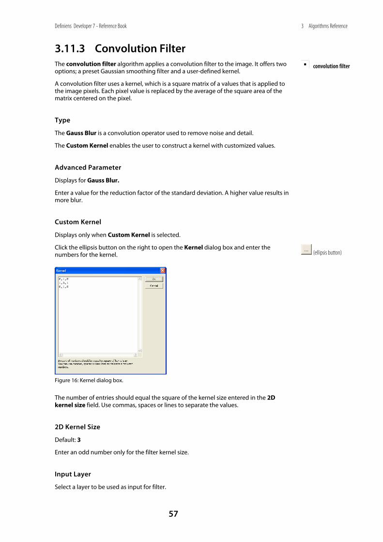
Definiens Developer 7 - Reference Book
57
3 Algorithms Reference
3.11.3 Convolution Filter The convolution filter algorithm applies a convolution filter to the image. It offers two options; a preset Gaussian smoothing filter and a user-defined kernel.
A convolution filter uses a kernel, which is a square matrix of a values that is applied to the image pixels. Each pixel value is replaced by the average of the square area of the matrix centered on the pixel.
Type
The Gauss Blur is a convolution operator used to remove noise and detail.
The Custom Kernel enables the user to construct a kernel with customized values.
Advanced Parameter
Displays for Gauss Blur.
Enter a value for the reduction factor of the standard deviation. A higher value results in more blur.
Custom Kernel
Displays only when Custom Kernel is selected.
Click the ellipsis button on the right to open the Kernel dialog box and enter the numbers for the kernel.
Figure 16: Kernel dialog box.
The number of entries should equal the square of the kernel size entered in the 2D kernel size field. Use commas, spaces or lines to separate the values.
2D Kernel Size
Default: 3
Enter an odd number only for the filter kernel size.
Input Layer
Select a layer to be used as input for filter.
convolution filter
(ellipsis button)
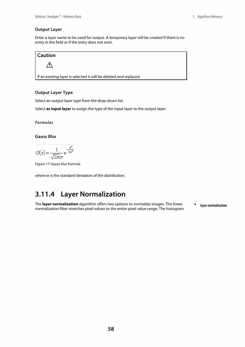
Definiens Developer 7 - Reference Book
58
3 Algorithms Reference
Output Layer
Enter a layer name to be used for output. A temporary layer will be created if there is no entry in the field or if the entry does not exist.
Caution
If an existing layer is selected it will be deleted and replaced.
Output Layer Type
Select an output layer type from the drop-down list.
Select as input layer to assign the type of the input layer to the output layer.
Formulas
Gauss Blur
Figure 17: Gauss blur formula.
where σ is the standard deviation of the distribution.
3.11.4 Layer Normalization The layer normalization algorithm offers two options to normalize images. The linear normalization filter stretches pixel values to the entire pixel value range. The histogram
layer normalization
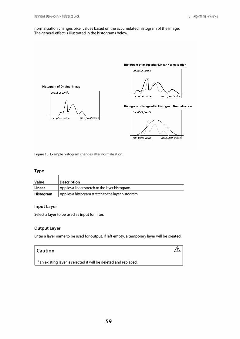
Definiens Developer 7 - Reference Book
59
3 Algorithms Reference
normalization changes pixel values based on the accumulated histogram of the image. The general effect is illustrated in the histograms below.
Figure 18: Example histogram changes after normalization.
Type
Value Description Linear Applies a linear stretch to the layer histogram.
Histogram Applies a histogram stretch to the layer histogram.
Input Layer
Select a layer to be used as input for filter.
Output Layer
Enter a layer name to be used for output. If left empty, a temporary layer will be created.
Caution
If an existing layer is selected it will be deleted and replaced.
Definiens Developer 7 - Reference Book
60
3 Algorithms Reference
3.11.5 Median Filter Use the median filter algorithm to replace the pixel value with the median value of neighboring pixels.
The median filter may preserve image detail better than a mean filter. Both can be used to reduce noise.
2D Kernel Size
Enter a number to set the kernel size in one slice.
Default: 3
Input Layer
Use the drop-down list to select a layer to be used as input for filter.
Output Layer
Enter a name for the or use the drop-down list to select a layer name to be used for output. If left empty, a temporary layer will be created.
Caution
If an existing layer is selected it will be deleted and replaced.
3.11.6 Pixel Frequency Filter The pixel frequency filter algorithm scans the input layer and select the color that is found in the greatest number of pixels. The frequency is checked in the area defined by the size of the kernel.
2D Kernel Size
Enter a number to set the kernel size.
Default: 3
Input Layer
Select a layer to be used as input for filter.
Output Layer
Enter a layer name to be used for output. If left empty, a layer will be created.
Caution
If an existing layer is selected it will be deleted and replaced.
median filter
pixel frequency filter
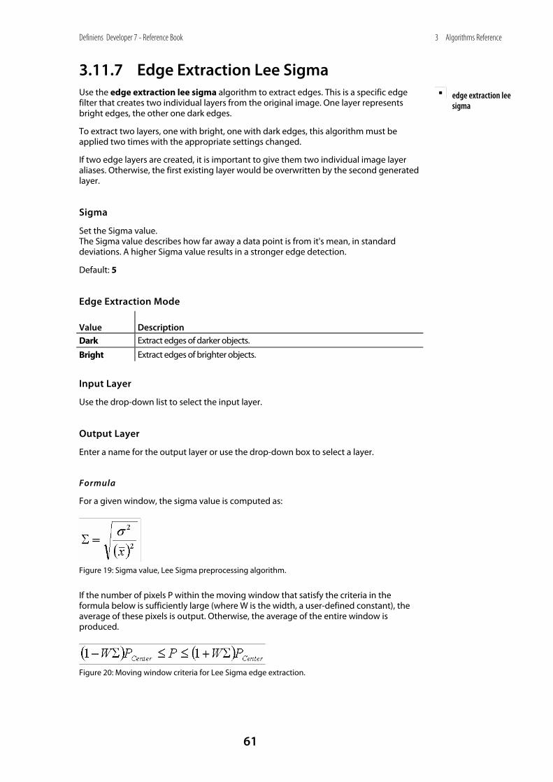
Definiens Developer 7 - Reference Book
61
3 Algorithms Reference
3.11.7 Edge Extraction Lee Sigma Use the edge extraction lee sigma algorithm to extract edges. This is a specific edge filter that creates two individual layers from the original image. One layer represents bright edges, the other one dark edges.
To extract two layers, one with bright, one with dark edges, this algorithm must be applied two times with the appropriate settings changed.
If two edge layers are created, it is important to give them two individual image layer aliases. Otherwise, the first existing layer would be overwritten by the second generated layer.
Sigma
Set the Sigma value. The Sigma value describes how far away a data point is from it's mean, in standard deviations. A higher Sigma value results in a stronger edge detection.
Default: 5
Edge Extraction Mode
Value Description Dark Extract edges of darker objects.
Bright Extract edges of brighter objects.
Input Layer
Use the drop-down list to select the input layer.
Output Layer
Enter a name for the output layer or use the drop-down box to select a layer.
Formula
For a given window, the sigma value is computed as:
Figure 19: Sigma value, Lee Sigma preprocessing algorithm.
If the number of pixels P within the moving window that satisfy the criteria in the formula below is sufficiently large (where W is the width, a user-defined constant), the average of these pixels is output. Otherwise, the average of the entire window is produced.
Figure 20: Moving window criteria for Lee Sigma edge extraction.
edge extraction lee sigma
Definiens Developer 7 - Reference Book
62
3 Algorithms Reference
3.11.8 Edge Extraction Canny Use the edge extraction canny filter algorithm to enhance or extract feature boundaries, using Canny's algorithm. Edge extraction filters may be used to enhance or extract feature boundaries. The resulting layer typically shows high pixel values where there is a distinctive change of pixel values in the original image layer.
Algorithm
The Canny Algorithm is provided.
Lower Threshold
Lower Threshold is applied after Higher Threshold. During the first step, edges are detected and pixels with values lower than Higher Threshold are removed from detected edges. During the final step, non-edge pixels (those previously removed because values were less than Higher Threshold) with values higher than Lower Threshold are marked as edge nodes again.
After applying the algorithm the first time, you can check results (edge pixel values) and the value for the threshold.
Usually values for this field are from 0.0 to 5.0.
Default: 0
Higher Threshold
After edges are detected, pixels with values lower than this threshold will not be marked as edge pixels. This allows removal of low intensity gradient edges from results.
After applying the algorithm once, users can check the results (values of edge pixels) and find the correct value for the threshold.
Usually values for this field are from 0.0 to 5.0.
Default: 0
Gauss Convolution FWHM
Enter the width of the Gaussian filter in relation to full width at half maximum of the Gaussian filter. This field determines the level of details covered by Gaussian filter. A higher value will produce a wider Gaussian filter and less detail will remain for edge detection. Thus, only high intensity gradient edges will be detected by Canny's algorithm.
Range of the field is 0.0001 till 15.0.
Default: 1.0
Input Layer
Use the drop-down list to select a layer to use for input.
Output Layer
Use the drop-down list to select a layer to use for output or enter a new name. Output is 32 Bit float. If the name of an existing 32Bit float temporary layer is entered or selected, it
edge extraction canny

Definiens Developer 7 - Reference Book
63
3 Algorithms Reference
will be used. If there is an existing temporary layer with a matching name but of a different type, it will be recreated.
Sample Results
Original Layer Lower Threshold: 0 Higher Threshold: 0 Gauss Convolution FWHM: 0.2
Lower Threshold: 0.3 Higher Threshold: 0.6 Gauss Convolution FWHM: 0.2
Lower Threshold: 0.3 Higher Threshold: 0.69 Gauss Convolution FWHM: 0.2
3.11.9 Surface Calculation Use the surface calculation algorithm to derive the slope for each pixel of a digital elevation model (DEM). This can be used to determine whether an area within a landscape is flat or steep and is independent from the absolute height values.
There is also an option to calculate aspect using Horn's Method.
Layer
Select the layer to which the filter will be applied.
Algorithm
Value Description
Slope Zevenbergen, Thorne (ERDAS)
Uses the Zevenbergen Thorne method to calculate slope. See: Quantitative analysis of land surface topography.
Zevenbergen, L W; Thorne, C R
Earth Surface Processes and Landforms [EARTH SURF. PROCESS. LANDFORMS.], vol. 12, no. 1, pp. 47-56, 1987 #
Aspect (Horn's Method)
Uses Horn's Method to calculate aspect. See: Horn, B. K. P. (1981). Hill Shading and the Reflectance Map, Proceedings of the IEEE, 69(1):14-47.
Gradient Unit
Available for slope.
Select Percent or Degree from the drop-down list for the gradient unit.
surface calculation
Definiens Developer 7 - Reference Book
64
3 Algorithms Reference
Unit of Pixel Values
Enter the ratio of the pixel height to pixel size.
Input Layer
Use the drop-down list to select a layer for input.
Output Layer
Select a layer for output or enter a new name.
3.11.10 Layer Arithmetics The layer arithmetic algorithm uses a pixel-based operation that enables the merger of up to four layers by mathematical operations (+ – * /). The layer created displays the result of this mathematical operation. This operation is performed on the pixel level which means, that all pixels of the image layers are used.
For example Layer 2 can be subtracted from Layer 1. This would mean that whenever the same pixel value in both layers exist, the result would be 0.
Before or after the operation, the layers can be normalized. Furthermore, weights can be used for each individual layer to influence the result.
Layer Name
Select or enter a raster layer name to which the filter will be applied. A layer will be created if the entry does not match an existing layer.
Output Layer Data Type
Select a data type for the raster channel if it must be created:
• float
• int 8bit
• int 16bit
• int 32bit
Minimum Input Value
Enter the lowest value that will be replaced by the output value.
Default: 0
Maximum Input Value
Enter the lowest value that will be replaced by the output value.
Default: 255
layer arithmetics
Definiens Developer 7 - Reference Book
65
3 Algorithms Reference
Output Value
The value that will be written in the raster layer. May be a number or an expression. For example, to add Layer 1 and Layer 2, enter Layer 1 + Layer 2.
3.11.11 Line Extraction The line extraction algorithm creates a layer and classifies the pixels of the input layer according to their line filter signal strength.
Line Direction
Enter the direction of the extracted line in degrees, between 0 and 179.
Default: 0
Line Length
Enter the length of the extracted line.
Default: 12
Line Width
Enter the length of the extracted line.
Default: 4
Border Width
Enter the width of the homogeneous border at the side of the extracted line.
Default: 4
Max Similarity of Line to Border
Enter a value to specify the similarity of lines to borders.
Default: 0.9
Min. Pixel Variance
Enter a value to specify the similarity of lines to borders.
Use -1 to use the variance of the input layer.
Default: 0
Min. Mean Difference
Enter a value for the minimum mean difference of the line pixels to the border pixels. If positive, bright lines are detected. Use 0 to detect bright and dark lines.
Input Layer
Use the drop-down list to select the layer where lines are to be extracted.
line extraction

Definiens Developer 7 - Reference Book
66
3 Algorithms Reference
Output Layer
Enter or select a layer where the maximal line signal strength will be written.
3.11.12 Apply Pixel Filters with Image Layer Operation Algorithms
Use the Image Layer Operation algorithms to apply filters to image layers at the pixel level.
Before digital images are analyzed, preprocessing is usually a necessary step for optimal results, and typically includes radiometric correction.
In addition, filter techniques can be applied which may improve the quality of the extracted information.
In Definiens Developer the term preprocessing refers to the application of filters (such as Gaussian, edge detection, or slope calculation from a digital elevation model).
Image layer operation algorithms can be applied on an existing image layer or a combination of existing image layers, which means, the existing layers are used as the basis for the new layer to be created.
The identifier for a layer created by an image layer operation algorithm is recognized in the same way a physical layer is recognized; by its image layer alias. If a layer exists and any algorithm is programmed to create a layer with an existing alias, this existing layer is overwritten by the newly generated layer. Physical layers can not be overwritten with the described procedure.
The result is one or more new raster layers, which are generated by the algorithm. The newly generated layers can be accessed in the project in the same way as other image layers, which means that all features related to image layers can be applied.
To avoid excessive hard disk use, preprocessed layers are only available temporarily. When other temporary layers are no longer needed, they can be deleted with the delete image layer algorithm.
Preprocessed layers are typically used within the segmentation process or for the classification process and can be used to improved the quality of the information extraction.
The key to the use of preprocessed layers is to be clear when they might be useful in a segmentation or classification step and when they would not. For example, if a multiresolution segmentation is executed with the goal of extracting a certain feature that is mainly distinguished by its spectral properties, the preprocessed layer should not be used in this step, because the image layer properties would influence the image object primitives. In this situation, the preprocessed layer might be used in the classification step, where it could help distinguish two features with similar spectral properties.
3.12 Thematic Layer Operation Algorithms
Thematic layer operation algorithms are used to transfer data from thematic layers to image objects and vice versa.
Definiens Developer 7 - Reference Book
67
3 Algorithms Reference
3.12.1 Synchronize Image Object Hierarchy
Change an image object level to exactly represent the thematic layer. Image objects smaller than the overlapping thematic object will be merged, image objects intersecting with several thematic objects will be cut.
Thematic Layers
Select the Thematic layers for the algorithm.
3.12.2 Read Thematic Attributes
Create and assign local image object variables according to a thematic layer attribute table. A variable with the same name as the thematic attribute will be created, attached to each image object in the domain and filled with the value given by the attribute table.
Thematic Layer
Select the Thematic layer for the algorithm.
Thematic Layer Attributes
Choose attributes from the thematic layer for the algorithm. You can select any numeric attribute from the attribute table of the selected thematic layer.
3.12.3 Write Thematic Attributes
Generate a attribute column entry from an image object feature. The updated attribute table can be saved to a .shp file.
Thematic Layer
Select the Thematic layers for the algorithm.
Feature
Select the feature for the algorithm.
Save Changes to File
If the thematic layer is linked with a shape file the changes can be updated to the file.
3.13 Export Algorithms Export algorithms are used to export table data, vector data and images derived from the image analysis results.
synchronize image object hierarchy
read thematic attributes
write thematic attributes

Definiens Developer 7 - Reference Book
68
3 Algorithms Reference
3.13.1 Export Classification View
Export the classification view to a raster file.
Export Item Name
Use default name or edit it.
Export Unclassified as Transparent
Activate to export unclassified image objects as transparent pixels.
Enable Geo Information
Activate to add geographic information.
Desktop File Format
Select the export file type used for desktop processing. If the algorithm is run in desktop mode, files will stored in this format. In server processing mode, the file format is defined in the export settings specified in the workspace.
Desktop Export Folder
Specify the file export folder used for desktop processing. If the algorithm is run in desktop mode, files will stored at this location. In server processing mode, the file location is defined in the export settings specified in the workspace.
3.13.2 Export Current View
Export the current project view to a raster file.
Export Item Name
Use default name or edit it.
Enable GEO Information
Activate to add GEO information.
Save Current View Settings
Click the ellipsis button to capture current view settings. Transparency settings may affect the appearance of the exported view as explained in the note following.
export classification view
export current view
(ellipsis button)
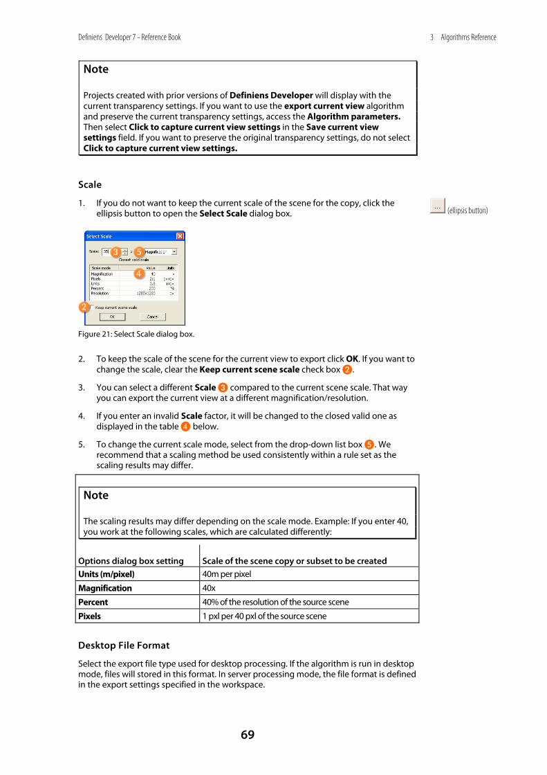
Definiens Developer 7 - Reference Book
69
3 Algorithms Reference
Note
Projects created with prior versions of Definiens Developer will display with the current transparency settings. If you want to use the export current view algorithm and preserve the current transparency settings, access the Algorithm parameters. Then select Click to capture current view settings in the Save current view settings field. If you want to preserve the original transparency settings, do not select Click to capture current view settings.
Scale
1. If you do not want to keep the current scale of the scene for the copy, click the ellipsis button to open the Select Scale dialog box.
Figure 21: Select Scale dialog box.
2. To keep the scale of the scene for the current view to export click OK. If you want to change the scale, clear the Keep current scene scale check box _.
3. You can select a different Scale ` compared to the current scene scale. That way you can export the current view at a different magnification/resolution.
4. If you enter an invalid Scale factor, it will be changed to the closed valid one as displayed in the table a below.
5. To change the current scale mode, select from the drop-down list box b. We recommend that a scaling method be used consistently within a rule set as the scaling results may differ.
Note
The scaling results may differ depending on the scale mode. Example: If you enter 40, you work at the following scales, which are calculated differently:
Options dialog box setting Scale of the scene copy or subset to be created
Units (m/pixel) 40m per pixel
Magnification 40x
Percent 40% of the resolution of the source scene
Pixels 1 pxl per 40 pxl of the source scene
Desktop File Format
Select the export file type used for desktop processing. If the algorithm is run in desktop mode, files will stored in this format. In server processing mode, the file format is defined in the export settings specified in the workspace.
(ellipsis button)

Definiens Developer 7 - Reference Book
70
3 Algorithms Reference
Desktop Export Folder
Specify the file export folder used for desktop processing. If the algorithm is run in desktop mode, files will stored at this location. In server processing mode, the file location is defined in the export settings specified in the workspace.
3.13.3 Export Thematic Raster Files
Export thematic raster files.
Export Item Name
Use default name or edit it.
Export Type
Select the type of export:
Value Description
Image Objects Export feature values.
Classification Export classification by unique numbers associated with classes.
Features
Select one or multiple features for exporting their values.
Desktop File Format
Select the export file type used for desktop processing. If the algorithm is run in desktop mode, files will stored in this format. In server processing mode, the file format is defined in the export settings specified in the workspace.
Desktop Export Folder
Specify the file export folder used for desktop processing. If the algorithm is run in desktop mode, files will stored at this location. In server processing mode, the file location is defined in the export settings specified in the workspace.
3.13.4 Export Domain Statistics
Select an image object domain and export statistics regarding selected features to a file.
Export Item Name
Use default name or edit it.
Features
Select one or multiple features for exporting their values.
export thematic raster files
export domain statistics

Definiens Developer 7 - Reference Book
71
3 Algorithms Reference
Desktop File Format
Select the export file type used for desktop processing. If the algorithm is run in desktop mode, files will stored in this format. In server processing mode, the file format is defined in the export settings specified in the workspace.
Desktop Export Folder
Specify the file export folder used for desktop processing. If the algorithm is run in desktop mode, files will stored at this location. In server processing mode, the file location is defined in the export settings specified in the workspace.
Statistical Operations
Select the statistical operators with a Yes or No from the drop-down arrow.
• Number
• Sum
• Mean
• Std. Dev.
• Min
• Max
3.13.5 Export Project Statistics
Export values of selected project features to a file.
Export Item Name
Use default name or edit it.
Features
Select one or multiple features for exporting their values.
Desktop File Format
Select the export file type used for desktop processing. If the algorithm is run in desktop mode, files will stored in this format. In server processing mode, the file format is defined in the export settings specified in the workspace.
Desktop Export Folder
Specify the file export folder used for desktop processing. If the algorithm is run in desktop mode, files will stored at this location. In server processing mode, the file location is defined in the export settings specified in the workspace.
export project statistics
Definiens Developer 7 - Reference Book
72
3 Algorithms Reference
3.13.6 Export Object Statistics
Export image object statistics of selected features to file. This generates one file per project.
Export Item Name
Use default name or edit it.
Features
Select one or multiple features for exporting their values.
Desktop File Format
Select the export file type used for desktop processing. If the algorithm is run in desktop mode, files will stored in this format. In server processing mode, the file format is defined in the export settings specified in the workspace.
Desktop Export Folder
Specify the file export folder used for desktop processing. If the algorithm is run in desktop mode, files will stored at this location. In server processing mode, the file location is defined in the export settings specified in the workspace.
3.13.7 Export Object Statistics for Report
Export image object statistics to a file. This generates one file per workspace.
Export Item Name
Use the default name or edit it.
Features
Select one or multiple features for exporting their values.
Desktop File Format
Select the export file type used for desktop processing. If the algorithm is run in desktop mode, files will stored in this format. In server processing mode, the file format is defined in the export settings specified in the workspace.
Desktop Export Folder
Specify the file export folder used for desktop processing. If the algorithm is run in desktop mode, files will stored at this location. In server processing mode, the file location is defined in the export settings specified in the workspace.
export object statistics
export object statistics for report

Definiens Developer 7 - Reference Book
73
3 Algorithms Reference
3.13.8 Export Vector Layers
Export vector layers to file.
Export Name
Use default name or edit it.
Features
Select one or multiple features for exporting their values.
Shape Type
Select a type of shapes for export:
• Polygons
• Lines
• Points
Export Type
Select a type of export:
• Center of main line
• Center of gravity
Desktop File Format
Select the export file type used for desktop processing. If the algorithm is run in desktop mode, files will stored in this format. In server processing mode, the file format is defined in the export settings specified in the workspace.
Desktop Export Folder
Specify the file export folder used for desktop processing. If the algorithm is run in desktop mode, files will stored at this location. In server processing mode, the file location is defined in the export settings specified in the workspace.
Write Shape Attr to CSV File
The column width for data in .dbf files is 255 characters.
Yes: Save the shape attributes as .csv file.
No: Save the shape attributes as .dbf file.
export vector layers

Definiens Developer 7 - Reference Book
74
3 Algorithms Reference
3.13.9 Export Image Object View
Export an image file for each image object.
Export Item Name
Use default name or edit it.
Border Size Around Object
Add pixels around the bounding box of the exported image object. Define the size of this bordering area.
Desktop File Format
Select the export file type used for desktop processing. If the algorithm is run in desktop mode, files will stored in this format. In server processing mode, the file format is defined in the export settings specified in the workspace.
Desktop Export Folder
Specify the file export folder used for desktop processing. If the algorithm is run in desktop mode, files will stored at this location. In server processing mode, the file location is defined in the export settings specified in the workspace.
Save Current View Settings
Click the ellipsis button to capture current view settings.
3.14 Workspace Automation Algorithms Workspace automation algorithms are used for working with subroutines of rule sets. These algorithms enable you to automate and accelerate the processing of workspaces with especially of large images. Workspace automation algorithms enable multi-scale workflows, which integrate analysis of images at different scales, magnifications, or resolutions.
3.14.1 Create Scene Copy
Create a scene copy that is a duplicate of a project with image layers and thematic layers, but without any results such as image objects, classes, or variables. This algorithm enables you to use subroutines.
Scene Name
Edit the name of the scene copy to be created.
export image object view
(ellipsis button)
create scene copy

Definiens Developer 7 - Reference Book
75
3 Algorithms Reference
Scale
1. If you do not want to keep the current scale of the scene for the copy, click the ellipsis button to open the Select Scale dialog box.
Figure 22: Select Scale dialog box.
2. To keep the scale of the scene for the copy click OK. If you want to change the scale, clear the Keep current scene scale check box _.
3. You can select a Scale ` different from the current scene scale, so you can work on the scene copy at a different magnification/resolution.
4. If you enter an invalid Scale factor, it will be changed to the closest valid scale as displayed in the table a below.
5. To change the current scale mode, select from the drop-down list box b. We recommend that you use the scaling method consistently within a rule set as the scaling results may differ.
Note
The scaling results may differ depending on the scale mode. Example: If you enter 40, you work at the following scales, which are calculated differently:
Options dialog box setting Scale of the scene copy or subset to be created
Units (m/pixel) 40m per pixel
Magnification 40x
Percent 40% of the resolution of the source scene
Pixels 1 pxl per 40 pxl of the source scene
Additional Thematic Layers
Edit the thematic layers you wish to load to a scene copy. This option is used to load intermediate result information that has been generated within a previous subroutine and exported to a geocoded thematic layer.
Use semicolons to separate multiple thematic layers, for example, ThematicLayer1.tif;ThematicLayer2.tif.
3.14.2 Create Scene Subset
Copy a portion (subset) of a scene as a project with a subset of image layers and thematic layers. The copy does not include results such as image objects, classes, or
(ellipsis button)
create scene subset

Definiens Developer 7 - Reference Book
76
3 Algorithms Reference
variables.
The algorithm uses the given coordinates (geocoding or pixel coordinates) of the source scene. You can create subset copies of an existing subset.
Scene Name
Edit the name of the copy of a scene subset to be created.
Scale
1. If you do not want to keep the current scale of the scene for the copy, click the ellipsis button to open the Select Scale dialog box.
Figure 23: Select Scale dialog box.
2. To keep the scale of the scene for the subset click OK.If you want to change the scale, clear the Keep current scene scale check box _.
3. You can select a different Scale ` compared to the current scene scale. That way you can work on the scene subset at a different magnification/resolution.
4. If you enter an invalid Scale factor, it will be changed to the closed valid one as displayed in the table a below.
5. To change the current scale mode, select from the drop-down list box b. We recommend that you use the scaling method consistently within a rule set as the scaling results may differ.
Note
The scaling results may differ depending on the scale mode. Example: If you enter 40, you work at the following scales, which are calculated differently:
Options dialog box setting Scale of the scene copy or subset to be created
Units (m/pixel) 40m per pixel
Magnification 40x
Percent 40% of the resolution of the source scene
Pixels 1 pxl per 40 pxl of the source scene
Additional Thematic Layers
Edit the thematic layers to load to a scene copy. This option is used to load intermediate result information which has been generated within a previous subroutine and exported to a geocoded thematic layer.
(ellipsis button)

Definiens Developer 7 - Reference Book
77
3 Algorithms Reference
Use semicolons to separate multiple thematic layers, for example ThematicLayer1.tif;ThematicLayer2.tif.
Define the Cutout
The cutout position is the portion of the scene to be copied.
Depending on the selected Image Object Domain of the process you can define the cutout position and size:
• Based on coordinates: If you select no image object in the Image Object Domain drop down list box, the given coordinates (geocoding or pixel coordinates) of the source scene are used.
• Based on classified image objects: If you select an image object level in the Image Object Domain drop down list box you can select classes of image objects. For each image object of the selected classes a subset is created based on a rectangular cutout area around the image object. Other image objects of the selected classes are commonly located inside the cutout rectangle, typically near the border. You can choose to include or to exclude them from further processing. Thus, you can extract regions of interest as separate subsets by extracting classified image objects as subset scenes.
Cutout Position Based on Coordinates
Min X Coord, Max X Coord, Min X Coord, Max-Y Coord
Edit the coordinates of the subset.
For the default Coordinates Orientation (below) of (0,0) in Lower left corner the different coordinates are defined as follows:
Figure 24: Coordinates of a subset.
The minimum X coordinates describes the left border.
The maximum X coordinates describes the right border.
The minimum Y coordinates describes the lower border.
The maximum Y coordinates describes the upper border.
Alternatively, click the drop-down arrow button to select from available variables. Entering a letter will open the Create Variable dialog box.
Coordinates Orientation
You can change the corner of the subset that is used as the calculation base for the coordinates. The default is (0,0) in Lower left corner.
(drop-down arrow button)
Definiens Developer 7 - Reference Book
78
3 Algorithms Reference
Cutout Position Based on Classified Image Objects
Border Size
Edit the size of the border in pixel that is added around the rectangular cutout area around the image objects when creating subsets from.
Exclude Other Image Objects
Commonly it occurs that other image objects of the selected classes are located inside the cutout rectangle, typically near the border. Select Yes to exclude them from further processing. For each scene subset, a .tif file is created describing the excluded areas as a no-data-mask. The .tif file is loaded as additional image layer to each scene subset project.
Desktop Export Folder
If Exclude Other Image Objects is selected, you can edit the file export folder used for desktop processing. If the algorithm is run in desktop mode, files will stored at this location. The default {:Scene.Dir} is the directory storing the image data.
In server processing mode, the file location is defined in the export settings specified in the workspace.
3.14.3 Create Scene Tiles
Create a tiled copy of the scene. Each tile is a separate project with its own image layers and thematic layers.
Together the tile projects represent the complete scene as it was before creating the tiled copy. The given coordinates (geocoding or pixel coordinates) of the source scene of the rule set are used. Results are not included before the tiles are processed.
After processing, you can stitch the tile results together and add them to the complete scene within the dimensions as it was before creating the tiled copy.
You can tile scenes and subsets several times.
Tile Width
Edit the width of the tiles to be created. Minimum with is 100 pixels.
Tile Height
Edit the height of the tiles to be created. Minimum height is 100 pixels.
3.14.4 Submit Scenes for Analysis
Execute a subroutine.
This algorithm enables you to connect subroutines with any process of the main process tree or other subroutines. You also can also choose whether to stitch the results of the analysis of subset copies.
create scene tiles
Submit Scenes for Analysis on page 78
submit scenes for analysis
Definiens Developer 7 - Reference Book
79
3 Algorithms Reference
Type of Scenes
Select the type of scene to submit to analysis: the Current Scene itself, Tiles, or Subsets and Copies.
Scene Name Prefix
Enter the prefix of the names of scene copies to be selected for submitting. A prefix is defined as the complete or the beginning of the scene name. Enter the unique part of the name to select only that scene, or the beginning of the name to select a group with similar or sequential names. For example, if you have scene names 7a, 7b and 7c, you can select them all by entering a 7, or select one by entering 7a, 7b or 7c.
Process Name
Address a subroutine or a process in the process tree of a subroutine for execution by using a slash mark / before hierarchy steps, for example, subroutine/process name.
Parameter Set for Processes
Select a parameter set to transfer variables to the following subroutines.
Percent of Tiles to Submit
If you do not want to submit all tiles for processing but only a certain percentage you can edit the percentage of tiles to be processed. If you change the default 100, the tiles are picked randomly. If the calculated number of tiles to be picked is not integer it is rounded up to the next integer.
Stitching Parameters
Stitch Subscenes
Select Yes to stitch the results of subscenes together and add them to the complete scene within its original dimensions.
Overlap Handling
If Subsets and Copies are stitched, the overlapping must be managed. You can opt to create Intersection image objects (default) or select Union to merge the overlapping image objects.
Class for Overlap Conflict
Overlapping image objects may have different classifications. In that case, you can define a class to be assigned to the image objects resulting from overlap handling.
Definiens Developer 7 - Reference Book
80
3 Algorithms Reference
Post-Processing
Request Post-Processes
Select Yes to execute another process.
Post-Process Name
Address a subroutine or a process in the process tree of a subroutine for execution by using a slash mark / before hierarchy steps, for example, subroutine/process name.
Parameter Set for Post-Processes
Select a parameter set to transfer variables to the following subroutines.
3.14.5 Delete Scenes Delete the scenes you do not want to use or store any more.
Type of Subscenes
Select the type of scene copy to be deleted: Tiles or Subsets and Copies.
Scene Name Prefix
Enter the prefix of the names of scene copies to be selected for deleting. A prefix is defined as the complete or the beginning of the scene name. Enter the unique part of the name to select only that scene, or the beginning of the name to select a group with similar or sequential names. For example, if you have scene names 7a, 7b and 7c, you can select them all by entering a 7, or select one by entering 7a, 7b or 7c.
3.14.6 Read Subscene Statistics
Read in exported result statistics and perform a defined mathematical summary operation. The resulting value is stored as a process variable that can be used for further calculations or export operations concerning the main scene.
This algorithm summarizes all values in the selected column in selected export item, using the selected summary type.
In cases the analysis of subscenes results in exporting statistics per each scene, the algorithm allows you to collect and merge the statistical results of multiple files. The advantage is that you do not need to stitch the subscenes results for result operations concerning the main scene.
Preconditions:
read subscene statistics
Definiens Developer 7 - Reference Book
81
3 Algorithms Reference
• For each subscene analysis, a project or domain statistic has been exported.
• All preceding subscene analysis including export has been processed completely before the read subscene statistics algorithm starts any result summary calculations. To ensure this, result calculations are done within a separate subroutine.
Type of Subscenes
Select the type of scene copy to summarize their results: Tiles or Subsets and Copies.
Scene Name Prefix
Enter the prefix of the names of scene copies to be selected for reading. A prefix is defined as the complete or the beginning of the scene name. Enter the unique part of the name to select only that scene, or the beginning of the name to select a group with similar or sequential names. For example, if you have scene names 7a, 7b and 7c, you can select them all by entering a 7, or select one by entering 7a, 7b or 7c.
Summary Type
Select the type of summary operation:
• Mean: Calculate the average of all values.
• Sum: Sum all values of appropriate statistics table columns.
• Std. Dev.: Calculates the standard deviation of all values.
• Min: Returns the minimal value of all values.
• Max: Returns the maximal value of all values.
Export Item
Enter the name of the export item as you defined it in the related exporting process of the subscenes (tiles or subsets).
Column
After defining the Export Item above, click the drop-down arrow button to select from the available columns from which values are read used for the summary operation.
Variable
Enter the name of the variable that stores the resulting value of the summary operation.
3.15 Customized Algorithms Customized algorithms enable you to reuse process sequences several times in one or different rule sets. Based on a developed process sequence, representing the developed code, you can create and reuse your own customized algorithms.
In contrast to duplicating a process, the main advantage of creating customized algorithms, is that when you want to modify the duplicated process you need to
(drop-down arrow button)

Definiens Developer 7 - Reference Book
82
3 Algorithms Reference
perform the changes to each instance of this process. However, with customized algorithms you only need to modify the customized algorithm template and the changes will take effect to every instance of this algorithm.
Note
Customized algorithms are created within the Process Tree window. They do not appear within the Algorithm drop-down list box in the Edit Process dialog box unless you first created them.
User Guide section: Reuse Process Sequences with Customized Algorithms
Definiens Developer 7 - Reference Book
83
4 Features Reference
4 Features Reference Contents in This Chapter About Features as a Source of Information 83
Basic Features Concepts 83
Object Features 95
Class-Related Features 163
Scene Features 173
Process-Related Features 178
Customized 181
[name of a metadata item] 181
Metadata 181
Feature Variables 182
Use Customized Features 182
Use Variables as Features 188
About Metadata as a Source of Information 188
Table of Feature Symbols 189
This Features Reference lists all available features in detail.
4.1 About Features as a Source of Information
Image objects have spectral, shape, and hierarchical characteristics. These characteristic attributes are called Features in Definiens software. Features are used as source of information to define the inclusion-or-exclusion parameters used to classify image objects.
There are two major types of features:
• Object features are attributes of image objects, for example the area of an image object.
• Global features are not connected to an individual image object, for example the number of image objects of a certain class.
4.2 Basic Features Concepts Basic features concepts offer an overview on concepts and basic definitions of features.
Definiens Developer 7 - Reference Book
84
4 Features Reference
4.2.1 Image Layer Related Features
4.2.1.1 Scene Scene is a rectangular area in a 2D space. It has an origin (x0, y0)geo, an extension sx in x, and an extension sy in y. The size of a pixel (in coordinate system unit) is denoted in ugeo.
If a scene is geocoded, (x0, y0)geo or in geo coordinates (in other words, these values refer to the coordination system defined by the geocoding).
If a scene contains pixel coordinates then (x0, y0) is its origin and sx, sy is its size (in pixels).
The formula is defined as follows:
xgeo = x0geo + xpxl * ugeo
ygeo = x0geo + ypxl * ugeo
Figure 25: Representation of a scene
Scenes can consist of an arbitrary number of image layers (k =1,...,K) and thematic layers (t=1,...,T).
Conversions of Feature Values
The conversion of feature values is handled differently, depending on the kind of values:
• Values identifying a position. These values are called position values.
• Values identifying certain distance measurements like Length or Area. These values are called unit values.
Conversion of Position Values
Position values can be converted from one coordinate system to another. The following position conversions are available:
• If the unit is Pixel, a position within the pixel coordinate system is identified.
• If the unit is Coordinate, a position within the user coordinate system is identified.
The position conversion is applied for image object features like Y center, Y max, X center and others.
Pixel Coordinate System on page 93
User Coordinate System on page 93
Definiens Developer 7 - Reference Book
85
4 Features Reference
Conversion of Unit Values
Distance values, like Length, Area and others are initially calculated in pixels. They can be converted to a distance unit.
To convert a pixel value to a unit, the following information is needed:
• Pixel size in meters.
• Value dimension, for example 1 for length, 2 for area and so forth.
• Unit factor, relative to the meter, for example 1 for meter, 100 for centimeter, 0.001 for kilometer and so forth
The following formula is valid for converting value from pixel to a unit:
u: pixel size in meters,
F: unit factor
dim: dimension
valunit = valpixel * udim * F
4.2.1.2 Image Layer The pixel value—that is the layer intensity—of an image layer k at pixel (x,y) is denoted as ck(x,y).
The dynamic range of image layers depends on the layer data type. The smallest possible value of an image layer is represented as ck
min, whereas the largest possible value as ck
max. The dynamic range is given by ckrange:=ck
max - ckmin. The supported layer data
types are:
Type ckmin ck
max ckrange
8-bit unsigned (int) 0 255 256
16-bit unsigned (int) 0 65535 65536
16-bit signed (int) -32767 32767 65535
32-bit unsigned (int) 0 4294967295 4294967296
32-bit signed (int) -2147483647 2147483647 4294967295
32-bit float 1.17e–38 3.40e+38 n/a
The mean value of all pixels of a layer is computed by:
The standard deviation of all pixels of a layer is computed by:
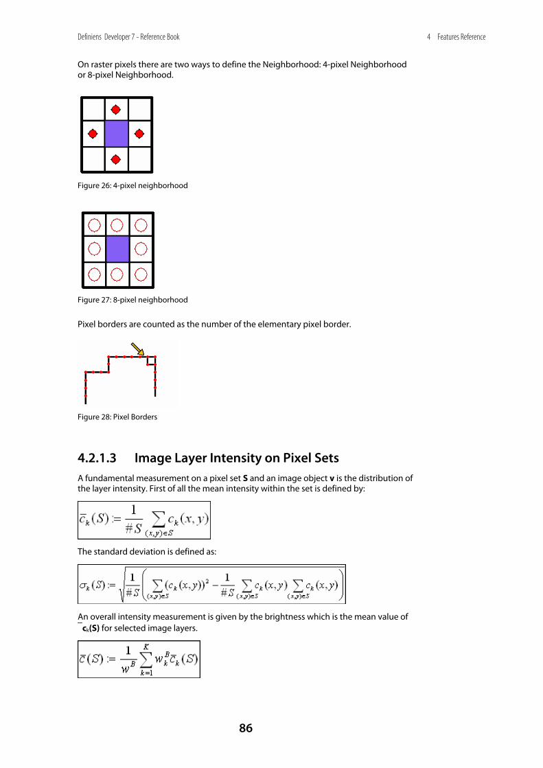
Definiens Developer 7 - Reference Book
86
4 Features Reference
On raster pixels there are two ways to define the Neighborhood: 4-pixel Neighborhood or 8-pixel Neighborhood.
Figure 26: 4-pixel neighborhood
Figure 27: 8-pixel neighborhood
Pixel borders are counted as the number of the elementary pixel border.
Figure 28: Pixel Borders
4.2.1.3 Image Layer Intensity on Pixel Sets A fundamental measurement on a pixel set S and an image object v is the distribution of the layer intensity. First of all the mean intensity within the set is defined by:
The standard deviation is defined as:
An overall intensity measurement is given by the brightness which is the mean value of ⎯ck(S) for selected image layers.

Definiens Developer 7 - Reference Book
87
4 Features Reference
If v is an image object and O a set of other image objects then the mean difference of the objects within O to an image object v is calculated by:
4.2.2 Image Object Related Features
4.2.2.1 Image Object Hierarchy An image object v or u is a 4-connected set of pixels in the scene. The pixels of an object v are denoted by Pv. The image objects are organized in levels (Vi, i=1,...,n) in where each object on each level creates a partition of the scene S.
•
•
The image object levels are hierarchically structured. This means that all image objects on a lower level are complete contained in exactly one image object of a higher level.
There are two types of feature distance:
• The level distance between image objects on different image object levels in the image object hierarchy.
• The spatial distance between objects on the same image object level in the image object hierarchy.
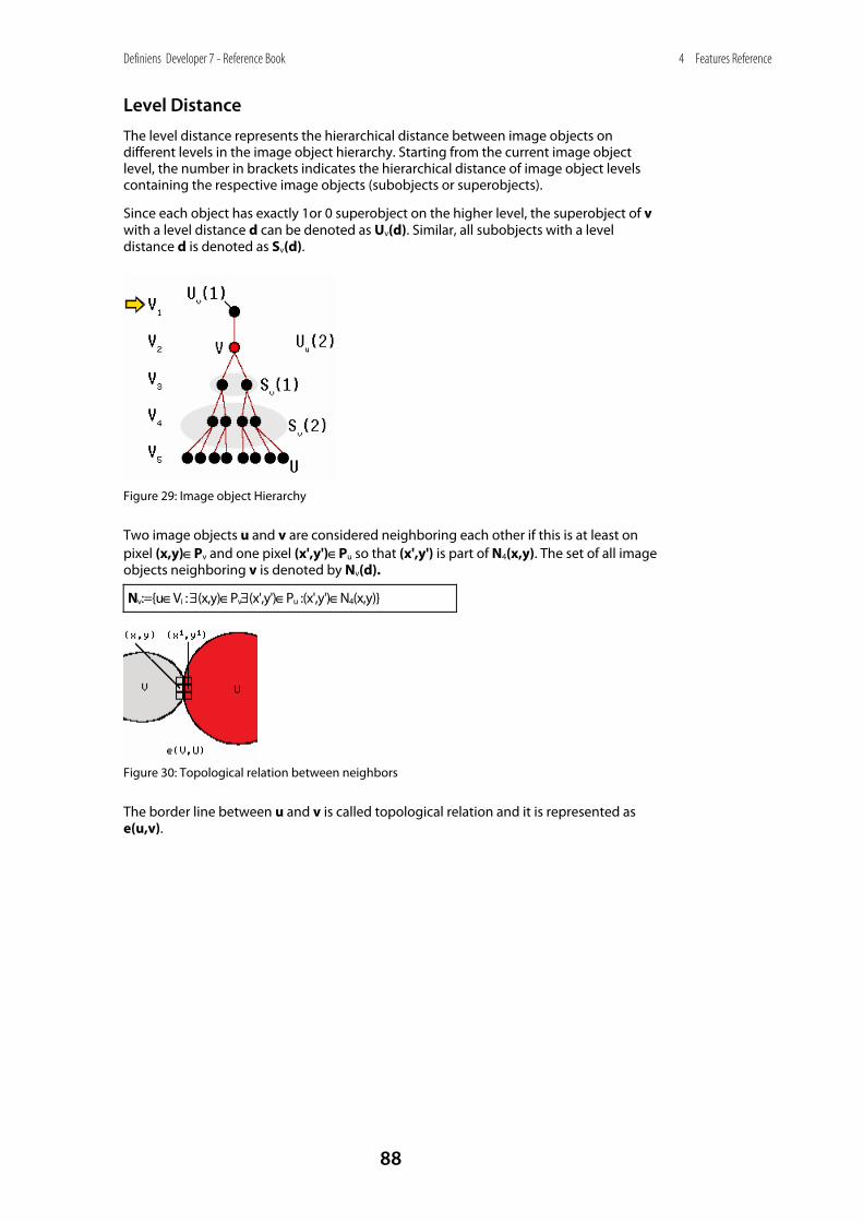
Definiens Developer 7 - Reference Book
88
4 Features Reference
Level Distance
The level distance represents the hierarchical distance between image objects on different levels in the image object hierarchy. Starting from the current image object level, the number in brackets indicates the hierarchical distance of image object levels containing the respective image objects (subobjects or superobjects).
Since each object has exactly 1or 0 superobject on the higher level, the superobject of v with a level distance d can be denoted as Uv(d). Similar, all subobjects with a level distance d is denoted as Sv(d).
Figure 29: Image object Hierarchy
Two image objects u and v are considered neighboring each other if this is at least on pixel (x,y)∈Pv and one pixel (x',y')∈Pu so that (x',y') is part of N4(x,y). The set of all image objects neighboring v is denoted by Nv(d).
Nv:={u∈Vi : ∃(x,y)∈Pv∃(x',y')∈Pu :(x',y')∈N4(x,y)}
Figure 30: Topological relation between neighbors
The border line between u and v is called topological relation and it is represented as e(u,v).
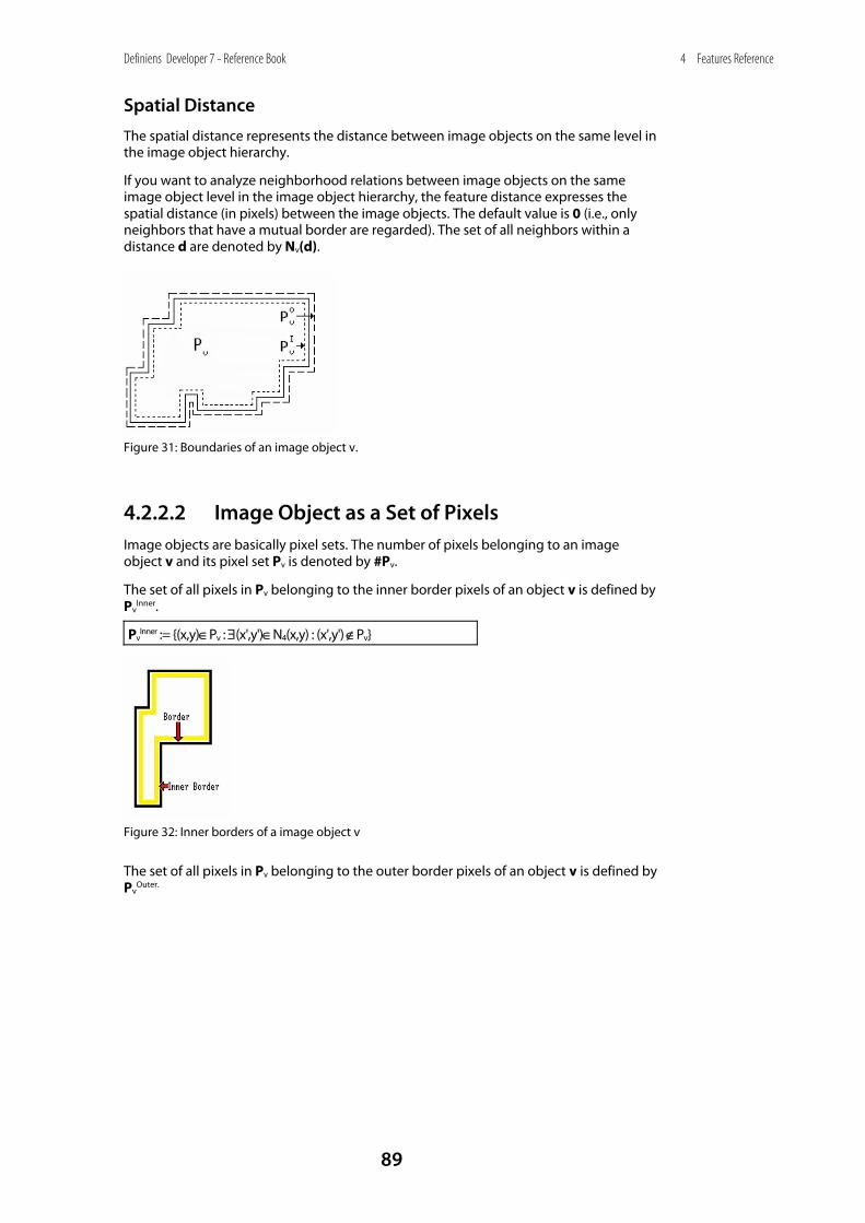
Definiens Developer 7 - Reference Book
89
4 Features Reference
Spatial Distance
The spatial distance represents the distance between image objects on the same level in the image object hierarchy.
If you want to analyze neighborhood relations between image objects on the same image object level in the image object hierarchy, the feature distance expresses the spatial distance (in pixels) between the image objects. The default value is 0 (i.e., only neighbors that have a mutual border are regarded). The set of all neighbors within a distance d are denoted by Nv(d).
Figure 31: Boundaries of an image object v.
4.2.2.2 Image Object as a Set of Pixels Image objects are basically pixel sets. The number of pixels belonging to an image object v and its pixel set Pv is denoted by #Pv.
The set of all pixels in Pv belonging to the inner border pixels of an object v is defined by Pv
Inner.
PvInner := {(x,y)∈Pv : ∃(x',y')∈N4(x,y) : (x',y') ∉Pv}
Figure 32: Inner borders of a image object v
The set of all pixels in Pv belonging to the outer border pixels of an object v is defined by Pv
Outer.
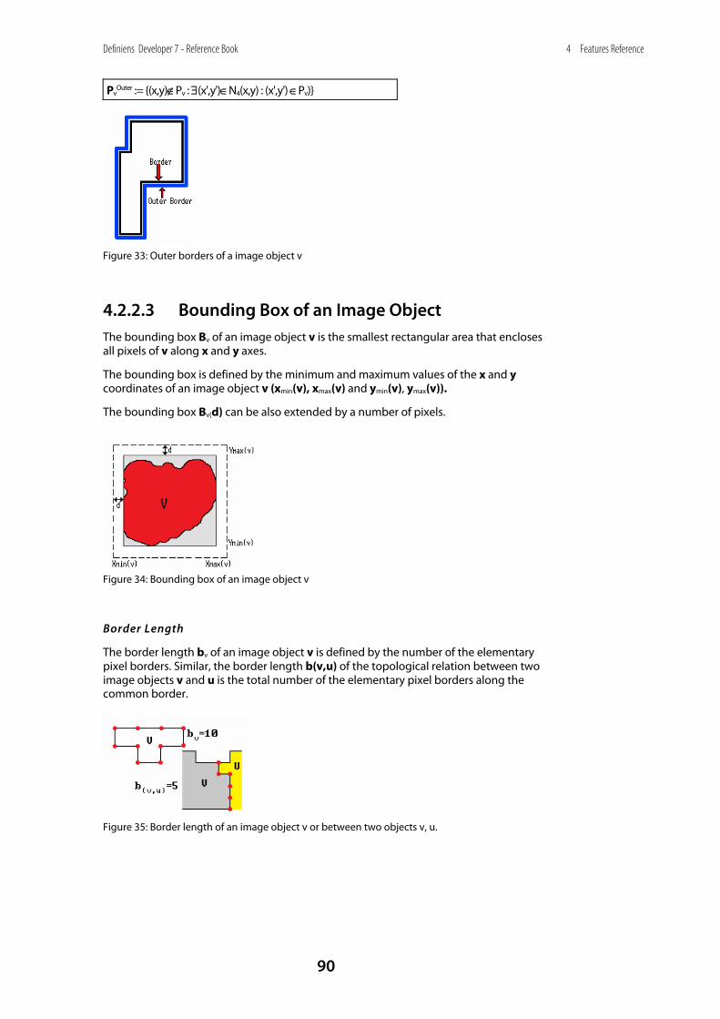
Definiens Developer 7 - Reference Book
90
4 Features Reference
PvOuter := {(x,y)∉Pv : ∃(x',y')∈N4(x,y) : (x',y') ∈Pv)}
Figure 33: Outer borders of a image object v
4.2.2.3 Bounding Box of an Image Object The bounding box Bv of an image object v is the smallest rectangular area that encloses all pixels of v along x and y axes.
The bounding box is defined by the minimum and maximum values of the x and y coordinates of an image object v (xmin(v), xmax(v) and ymin(v), ymax(v)).
The bounding box Bv(d) can be also extended by a number of pixels.
Figure 34: Bounding box of an image object v
Border Length
The border length bv of an image object v is defined by the number of the elementary pixel borders. Similar, the border length b(v,u) of the topological relation between two image objects v and u is the total number of the elementary pixel borders along the common border.
Figure 35: Border length of an image object v or between two objects v, u.
Definiens Developer 7 - Reference Book
91
4 Features Reference
4.2.3 Class-Related Features
4.2.3.1 Class-Related Sets
Let M=(m1,...,ma) be a set of classes with m being a specific class and m∈M. Each object has a fuzzy membership value of φ(v,m) to class m. In addition each image object also
carries the stored membership value that is computed during the last classification algorithm. By restricting a set of objects O to only the image object that belong to class m many interesting class related features can be computed:
Nv(d,m) := {u∈Nv(d) : =1}
Sv(d,m) := {u∈Sv(d) : =1}
Uv(d,m) := {u∈Uv(d) : =1}
Vi(m) := {u∈Vi(m) : =1}
For example, the mean difference of layer k to a neighbor object within a distance d and that object belongs to a class m is defined as ⎯Δk(v,Nv(d,m)).
4.2.4 Shape-Related Features Many of the form features provided by Definiens Developer are based on the statistics of the spatial distribution of the pixels that form an image object. As a central tool to work with these statistics Definiens Developer uses the covariance matrix:
Parameters:
• X = x-coordinates of all pixels forming the image object
• Y = y-coordinates of all pixels forming the image object
Formula:
Another frequently used technique to derive information about the form of image objects (especially length and width) is the bounding box approximation. Such a bounding box can be calculated for each image object and its geometry can be used as a first clue of the image object itself.
The main information provided by the bounding box is its length a, its width b, its area a * b and its degree of filling f, which is the area A covered by the image object divided by the total area a * b of the bounding box.
4.2.4.1 Shape Approximations based on Eigenvalues This approach measures the statistical distribution of the pixel coordinates (x,y) of a set Pv.
> Object Features > Shape
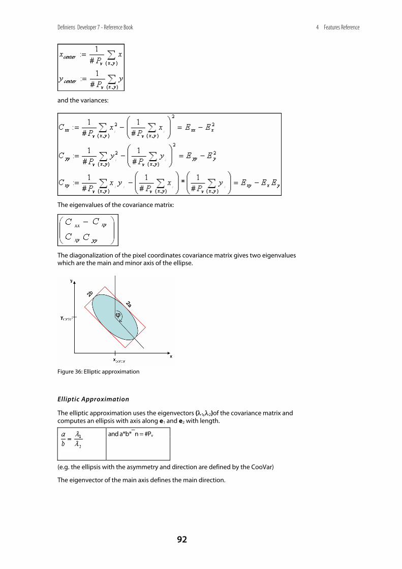
Definiens Developer 7 - Reference Book
92
4 Features Reference
and the variances:
The eigenvalues of the covariance matrix:
The diagonalization of the pixel coordinates covariance matrix gives two eigenvalues which are the main and minor axis of the ellipse.
Figure 36: Elliptic approximation
Elliptic Approximation
The elliptic approximation uses the eigenvectors (λ1,λ2)of the covariance matrix and computes an ellipsis with axis along e1 and e2 with length.
and a*b*⎯n = #Pv
(e.g. the ellipsis with the asymmetry and direction are defined by the CooVar)
The eigenvector of the main axis defines the main direction.
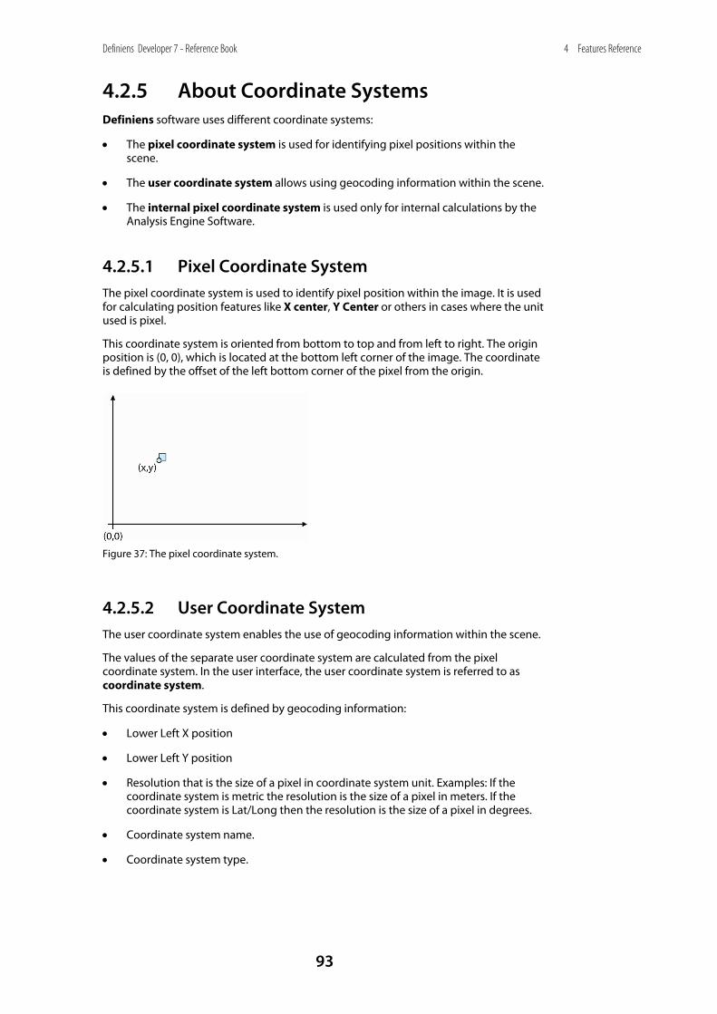
Definiens Developer 7 - Reference Book
93
4 Features Reference
4.2.5 About Coordinate Systems Definiens software uses different coordinate systems:
• The pixel coordinate system is used for identifying pixel positions within the scene.
• The user coordinate system allows using geocoding information within the scene.
• The internal pixel coordinate system is used only for internal calculations by the Analysis Engine Software.
4.2.5.1 Pixel Coordinate System The pixel coordinate system is used to identify pixel position within the image. It is used for calculating position features like X center, Y Center or others in cases where the unit used is pixel.
This coordinate system is oriented from bottom to top and from left to right. The origin position is (0, 0), which is located at the bottom left corner of the image. The coordinate is defined by the offset of the left bottom corner of the pixel from the origin.
Figure 37: The pixel coordinate system.
4.2.5.2 User Coordinate System The user coordinate system enables the use of geocoding information within the scene.
The values of the separate user coordinate system are calculated from the pixel coordinate system. In the user interface, the user coordinate system is referred to as coordinate system.
This coordinate system is defined by geocoding information:
• Lower Left X position
• Lower Left Y position
• Resolution that is the size of a pixel in coordinate system unit. Examples: If the coordinate system is metric the resolution is the size of a pixel in meters. If the coordinate system is Lat/Long then the resolution is the size of a pixel in degrees.
• Coordinate system name.
• Coordinate system type.
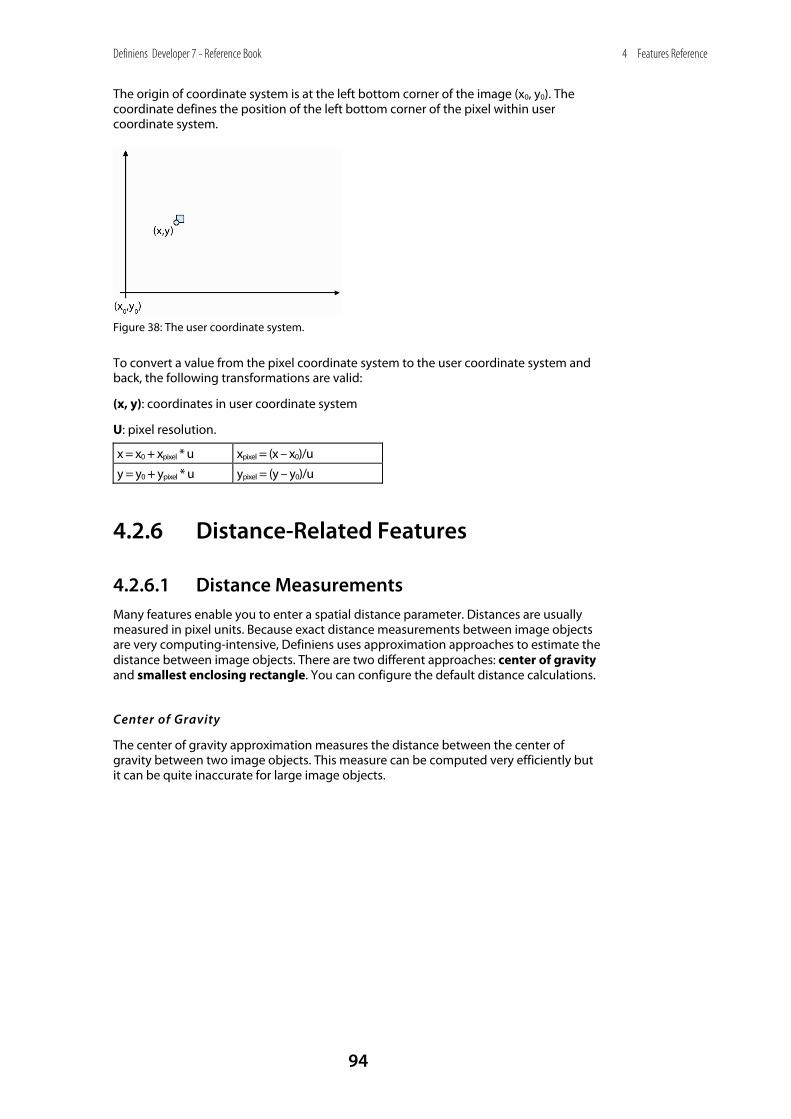
Definiens Developer 7 - Reference Book
94
4 Features Reference
The origin of coordinate system is at the left bottom corner of the image (x0, y0). The coordinate defines the position of the left bottom corner of the pixel within user coordinate system.
Figure 38: The user coordinate system.
To convert a value from the pixel coordinate system to the user coordinate system and back, the following transformations are valid:
(x, y): coordinates in user coordinate system
U: pixel resolution.
x = x0 + xpixel * u xpixel = (x – x0)/u
y = y0 + ypixel * u ypixel = (y – y0)/u
4.2.6 Distance-Related Features
4.2.6.1 Distance Measurements Many features enable you to enter a spatial distance parameter. Distances are usually measured in pixel units. Because exact distance measurements between image objects are very computing-intensive, Definiens uses approximation approaches to estimate the distance between image objects. There are two different approaches: center of gravity and smallest enclosing rectangle. You can configure the default distance calculations.
Center of Gravity
The center of gravity approximation measures the distance between the center of gravity between two image objects. This measure can be computed very efficiently but it can be quite inaccurate for large image objects.
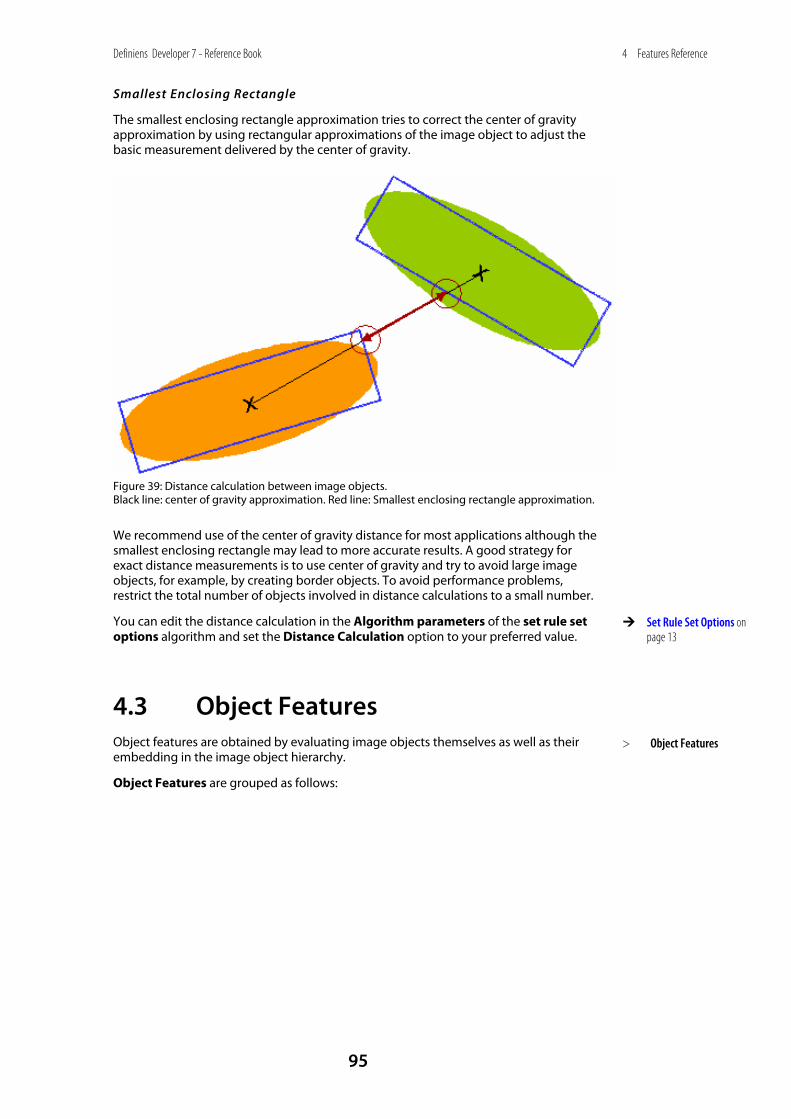
Definiens Developer 7 - Reference Book
95
4 Features Reference
Smallest Enclosing Rectangle
The smallest enclosing rectangle approximation tries to correct the center of gravity approximation by using rectangular approximations of the image object to adjust the basic measurement delivered by the center of gravity.
Figure 39: Distance calculation between image objects. Black line: center of gravity approximation. Red line: Smallest enclosing rectangle approximation.
We recommend use of the center of gravity distance for most applications although the smallest enclosing rectangle may lead to more accurate results. A good strategy for exact distance measurements is to use center of gravity and try to avoid large image objects, for example, by creating border objects. To avoid performance problems, restrict the total number of objects involved in distance calculations to a small number.
You can edit the distance calculation in the Algorithm parameters of the set rule set options algorithm and set the Distance Calculation option to your preferred value.
4.3 Object Features Object features are obtained by evaluating image objects themselves as well as their embedding in the image object hierarchy.
Object Features are grouped as follows:
Set Rule Set Options on page 13
> Object Features
Definiens Developer 7 - Reference Book
96
4 Features Reference
• Customized: All features created in the Edit Customized Feature dialog box referring to object features.
• Layer Values: Layer values evaluate the first and second statistical moment (mean and standard deviation) of an image object's pixel value and the object's relations to other image object's pixel values. Use these to describe image objects with information derived from their spectral properties.
• Shape: Shape features evaluate the image object's shape in a variety of respects. The basic shape features are calculated based on the object's pixels. Another type of shape features, based on sub-object analysis, is available as a result of the hierarchical structure. If image objects of a certain class stand out because of their shape, you are likely to find a form feature that describes them.
• Texture: The image object's texture can be evaluated using different texture features. New types of texture features based on an analysis of sub-objects. These are especially helpful for evaluating highly textured data. Likewise, a large number of features based upon the co-occurrence matrix after Haralick can be utilized.
• Variables: Define variables to describe interim values related to variables.
• Hierarchy: This feature provides information about the embedding of the image object in the image object hierarchy. These features are best suited for structuring a class hierarchy when you are working with an image object hierarchy consisting of more than one image object level.
• Thematic Attributes: If your project contains a thematic layer, the object's thematic properties (taken from the thematic layer) may be evaluated. Depending on the attributes of the thematic layer, a large range of different features become available.
4.3.1 Customized
[name of a customized feature]
If existing, customized features referring to object features are listed in the feature tree.
4.3.2 Layer Values
4.3.2.1 Mean
> Object Features > Customized
> Object Features > Customized > [name of a customized
feature]
> Object Features > Layer Values
> Object Features > Layer Values > Mean
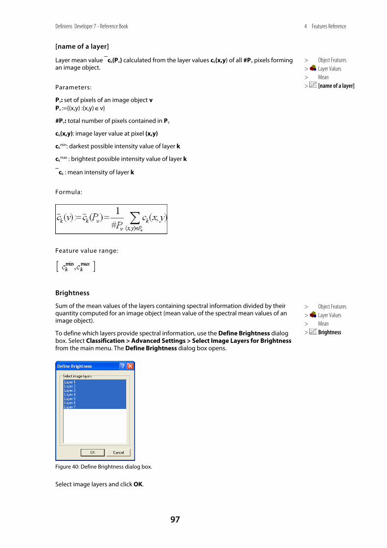
Definiens Developer 7 - Reference Book
97
4 Features Reference
[name of a layer]
Layer mean value ⎯ck(Pv) calculated from the layer values ck(x,y) of all #Pv pixels forming an image object.
Parameters:
Pv: set of pixels of an image object v Pv :={(x,y) :(x,y) ∈v}
#Pv: total number of pixels contained in Pv
ck(x,y): image layer value at pixel (x,y)
ckmin: darkest possible intensity value of layer k
ckmax : brightest possible intensity value of layer k
⎯ck : mean intensity of layer k
Formula:
Feature value range:
Brightness
Sum of the mean values of the layers containing spectral information divided by their quantity computed for an image object (mean value of the spectral mean values of an image object).
To define which layers provide spectral information, use the Define Brightness dialog box. Select Classification > Advanced Settings > Select Image Layers for Brightness from the main menu. The Define Brightness dialog box opens.
Figure 40: Define Brightness dialog box.
Select image layers and click OK.
> Object Features > Layer Values > Mean > [name of a layer]
> Object Features > Layer Values > Mean > Brightness
Definiens Developer 7 - Reference Book
98
4 Features Reference
Because combined negative and positive data values would create an erroneous value for brightness, this feature is only calculated with layers of positive values.
Parameters:
wkB: brightness weight of layer k
⎯ck(v): mean intensity of layer k of an image object v
ckmin: darkest possible intensity value of layer k
ckmax : brightest possible intensity value of layer k
Formula:
Feature value range:
Condition:
Feature available only for scenes with more than one layer.
Max. diff.
To calculate Max Diff. the minimum mean value belonging to an object is subtracted from its maximum value. To get the maximum and minimum value the means of all layers belonging to an object are compared with each other. Subsequently the result is divided by the brightness.
Parameters:
i, j : image layers
⎯c(v) : brightness
⎯ci(v) : mean intensity of layer i
⎯cj(v) : mean intensity of layer j
ckmax : brightest possible intensity value of layer k
KB : layers with positive brightness weight
KB :={k ∈ K : wk=1}, wk:layer weight
> Object Features > Layer Values > Mean > Max. diff.

Definiens Developer 7 - Reference Book
99
4 Features Reference
Formula:
Feature value range:
Normally, the values given to this range are between 0 and 1.
Conditions:
Feature available only for scenes with more than one layer.
If ⎯c(v)=0 then the formula is undefined.
4.3.2.2 Standard Deviation
[name of a layer]
Standard deviation calculated from the layer values of all n pixels forming an image object.
Parameters:
σk(v): standard deviation of layer k of an image object v
Pv: set of pixels of an image object v
#Pv: total number of pixels contained in Pv
ck(x,y): image layer value at pixel (x,y)
(x,y) : pixel coordinates
ckrange : data range of layer k
ckrange :=ck
max -ckmin
Formula:
Feature value range:
> Object Features > Layer Values > Standard Deviation
> Object Features > Layer Values > Standard Deviation > [name of a layer]
Definiens Developer 7 - Reference Book
100
4 Features Reference
4.3.2.3 Pixel Based
Ratio
The ratio of layer k reflects the amount that layer k contributes to the total brightness.
Parameters:
wkB: brightness weight of layer k
⎯ck(v): mean intensity of layer k of an image object v
⎯c(v): brightness
Formula:
If wkB=1 and c(v)≠0 then
If wkB=0 or ⎯c(v)=0 then the ratio is equal to 0.
Feature value range:
[0,1]
Conditions:
• For scenes with more than one layer.
• Only layers containing spectral information can be used to achieve reasonable results.
• Since combined negative and positive data values would create an erroneous value for ratio, this feature is only calculated with layers of positive values.
Note
The results get meaningless if the layers have different signed data types.
Min. pixel value
Value of the pixel with the minimum intensity value of the image object.
Parameters:
(x,y): pixel coordinates
ck(x,y): image layer value at pixel (x,y)
ckmin: darkest possible intensity value of layer k
ckmax : brightest possible intensity value of layer k
> Object Features > Layer Values > Pixel Based
> Object Features > Layer Values > Pixel Based > Ratio
> Object Features > Layer Values > Pixel Based > Min. pixel value
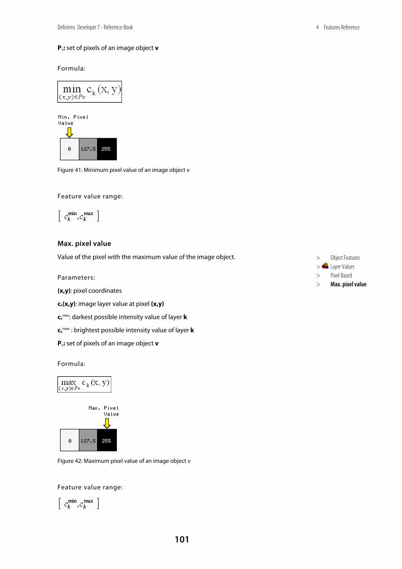
Definiens Developer 7 - Reference Book
101
4 Features Reference
Pv: set of pixels of an image object v
Formula:
Figure 41: Minimum pixel value of an image object v
Feature value range:
Max. pixel value
Value of the pixel with the maximum value of the image object.
Parameters:
(x,y): pixel coordinates
ck(x,y): image layer value at pixel (x,y)
ckmin: darkest possible intensity value of layer k
ckmax : brightest possible intensity value of layer k
Pv: set of pixels of an image object v
Formula:
Figure 42: Maximum pixel value of an image object v
Feature value range:
> Object Features > Layer Values > Pixel Based > Max. pixel value
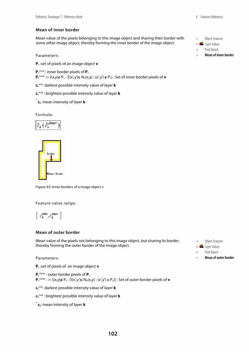
Definiens Developer 7 - Reference Book
102
4 Features Reference
Mean of inner border
Mean value of the pixels belonging to this image object and sharing their border with some other image object, thereby forming the inner border of the image object.
Parameters:
Pv :set of pixels of an image object v
PvInner : inner border pixels of Pv
PvInner := {(x,y)∈Pv : ∃(x',y')∈N4(x,y) : (x',y') ∉Pv} : Set of inner border pixels of v
ckmin: darkest possible intensity value of layer k
ckmax : brightest possible intensity value of layer k
⎯ck: mean intensity of layer k
Formula:
Figure 43: Inner borders of a image object v
Feature value range:
Mean of outer border
Mean value of the pixels not belonging to this image object, but sharing its border, thereby forming the outer border of the image object.
Parameters:
Pv :set of pixels of an image object v
PvOuter : outer border pixels of Pv
PvOuter : := {(x,y)∉Pv : ∃(x',y')∈N4(x,y) : (x',y') ∈Pv)} : Set of outer border pixels of v
ckmin: darkest possible intensity value of layer k
ckmax : brightest possible intensity value of layer k
⎯ck: mean intensity of layer k
> Object Features > Layer Values > Pixel Based > Mean of inner border
> Object Features > Layer Values > Pixel Based > Mean of outer border
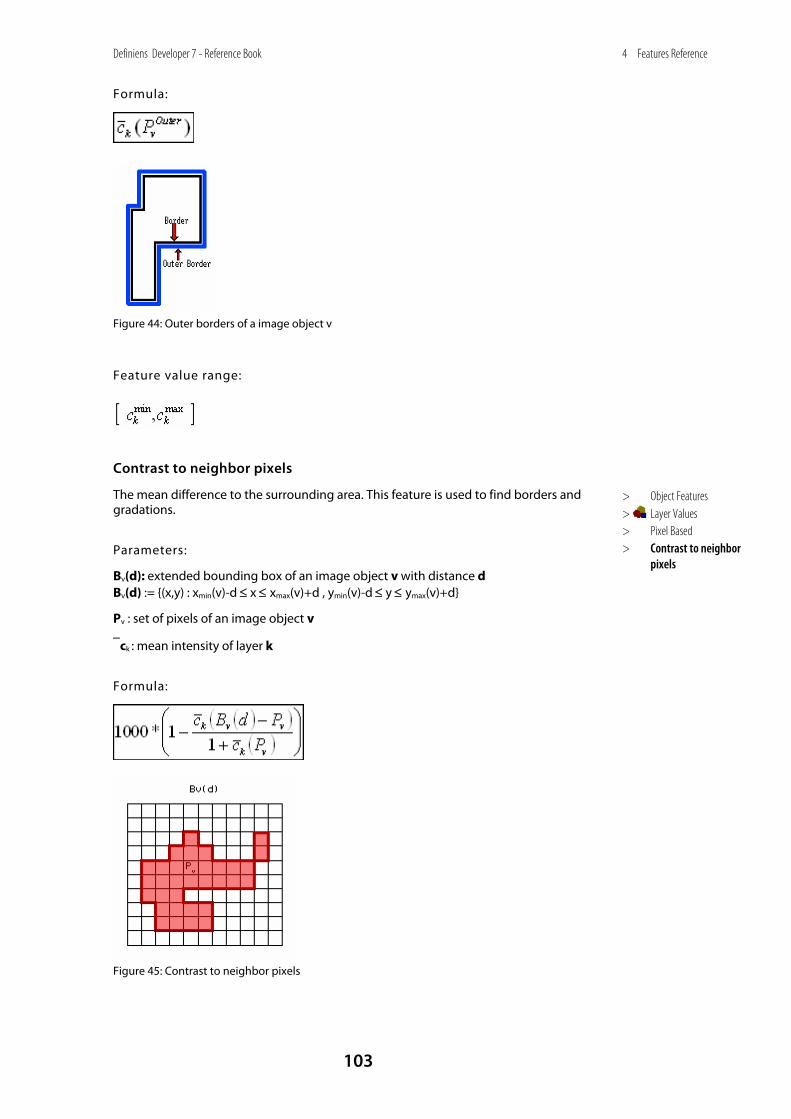
Definiens Developer 7 - Reference Book
103
4 Features Reference
Formula:
Figure 44: Outer borders of a image object v
Feature value range:
Contrast to neighbor pixels
The mean difference to the surrounding area. This feature is used to find borders and gradations.
Parameters:
Bv(d): extended bounding box of an image object v with distance d Bv(d) := {(x,y) : xmin(v)-d ≤ x ≤ xmax(v)+d , ymin(v)-d ≤ y ≤ ymax(v)+d}
Pv : set of pixels of an image object v
⎯ck : mean intensity of layer k
Formula:
Figure 45: Contrast to neighbor pixels
> Object Features > Layer Values > Pixel Based > Contrast to neighbor
pixels
Definiens Developer 7 - Reference Book
104
4 Features Reference
Feature value range:
[-1000, 1000]
Conditions:
• If d=0, then Bv(d)=Bv, and if Bv=Pv ∴ the formula is invalid.
• If unsigned data exist then maybe ⎯ck(Pv) = -1 ∴ the formula is invalid.
• If ⎯ck(Pv)=0 then the values are meaningless.
• The distance should always be greater than 0, (d>0).
Std. deviation to neighbor pixels
Computes the standard deviation of the pixels not belonging to the image object in the extended bounding box.
Parameters:
Pv :set of pixels of an image object v
Bv(d): extended bounding box of an image object v with distance d
Formula:
σk(Bv(d) - Pv)
Feature value range:
[0,ckmax/2]
Condition:
If d=0, then Bv(d)=Bv, and if Bv=Pv ∴ the formula is invalid.
4.3.2.4 To Neighbors
Mean diff. to neighbors
For each neighboring object the layer mean difference is computed and weighted with regard to the length of the border between the objects (if they are direct neighbors, feature distance = 0) or the area covered by the neighbor objects (if neighborhood is defined within a certain perimeter (in pixels) around the image object in question, feature distance > 0).
The mean difference to direct neighbors is calculated as follows:
Parameters:
u,v : image objects
b(v,u): topological relation border length
> Object Features > Layer Values > Pixel Based > StdDev. to neighbor
pixels
> Object Features > Layer Values > To Neighbors
> Object Features > Layer Values > To Neighbors > Mean diff. to neighbors
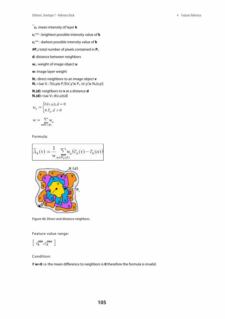
Definiens Developer 7 - Reference Book
105
4 Features Reference
⎯ck :mean intensity of layer k
ckmax : brightest possible intensity value of k
ckmin : darkest possible intensity value of k
#Pu: total number of pixels contained in Pu
d: distance between neighbors
wu: weight of image object u
w: image layer weight
Nv: direct neighbors to an image object v Nv:={u∈Vi : ∃(x,y)∈Pv∃(x',y')∈Pu :(x',y')∈N4(x,y)}
Nv(d): neighbors to v at a distance d Nv(d):={u∈Vi: d(v,u)≤d}
Formula:
Figure 46: Direct and distance neighbors.
Feature value range:
Condition:
If w=0 ⇒ the mean difference to neighbors is 0 therefore the formula is invalid.
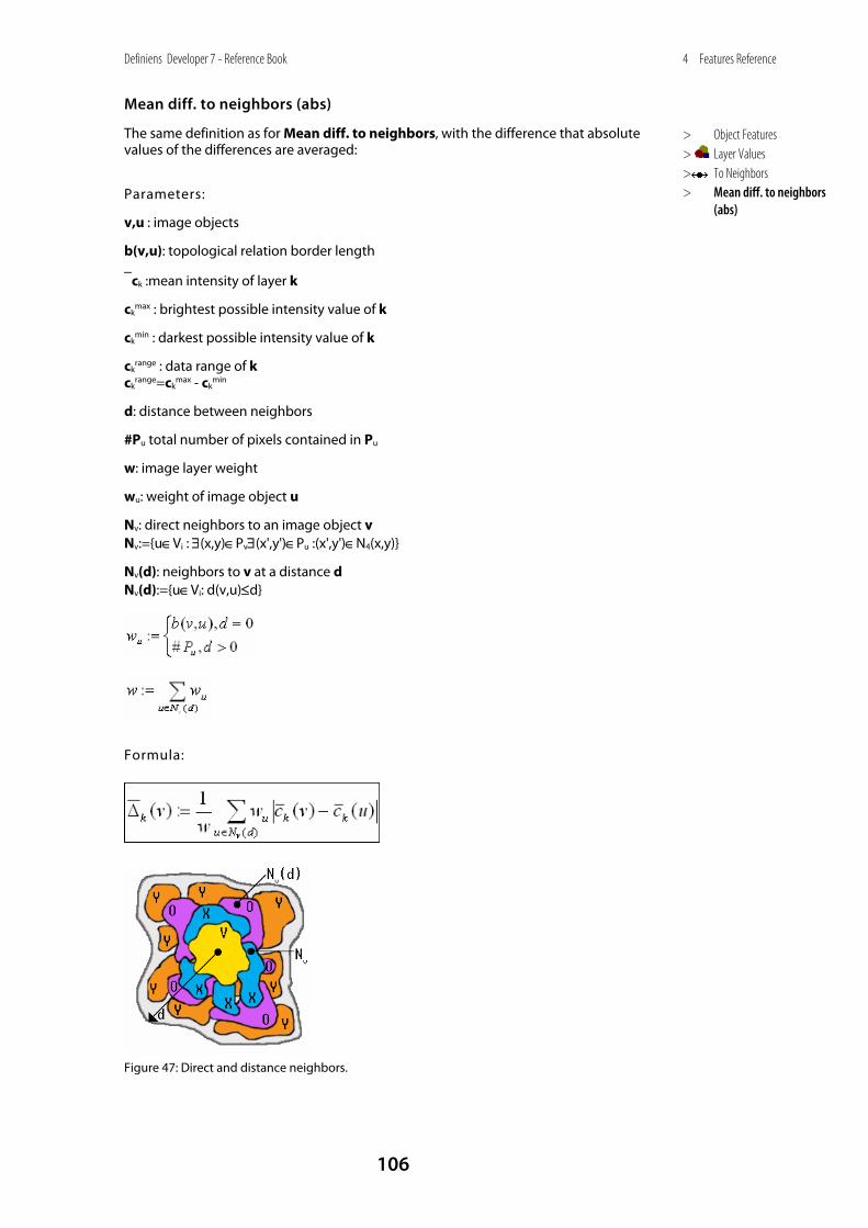
Definiens Developer 7 - Reference Book
106
4 Features Reference
Mean diff. to neighbors (abs)
The same definition as for Mean diff. to neighbors, with the difference that absolute values of the differences are averaged:
Parameters:
v,u : image objects
b(v,u): topological relation border length
⎯ck :mean intensity of layer k
ckmax : brightest possible intensity value of k
ckmin : darkest possible intensity value of k
ckrange : data range of k
ckrange=ck
max - ckmin
d: distance between neighbors
#Pu total number of pixels contained in Pu
w: image layer weight
wu: weight of image object u
Nv: direct neighbors to an image object v Nv:={u∈Vi : ∃(x,y)∈Pv∃(x',y')∈Pu :(x',y')∈N4(x,y)}
Nv(d): neighbors to v at a distance d Nv(d):={u∈Vi: d(v,u)≤d}
Formula:
Figure 47: Direct and distance neighbors.
> Object Features > Layer Values > To Neighbors > Mean diff. to neighbors
(abs)
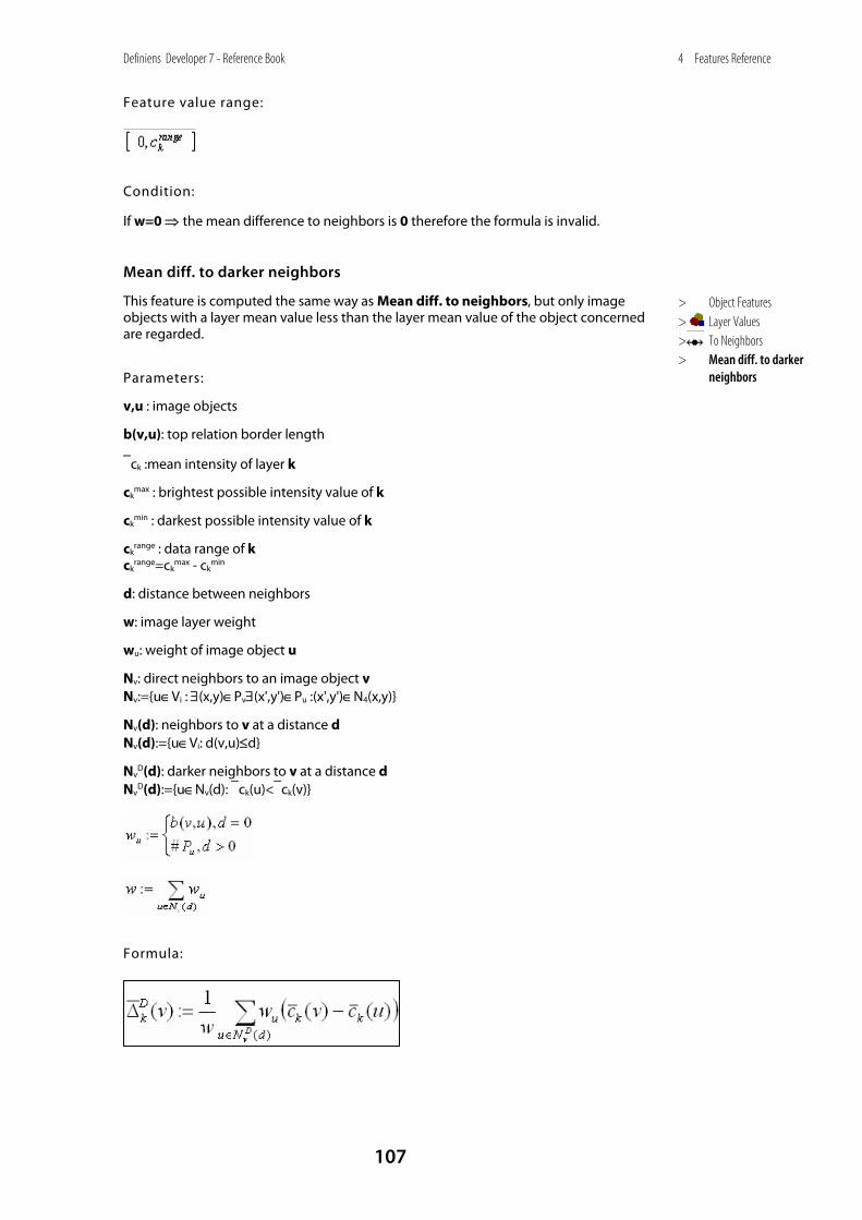
Definiens Developer 7 - Reference Book
107
4 Features Reference
Feature value range:
Condition:
If w=0 ⇒ the mean difference to neighbors is 0 therefore the formula is invalid.
Mean diff. to darker neighbors
This feature is computed the same way as Mean diff. to neighbors, but only image objects with a layer mean value less than the layer mean value of the object concerned are regarded.
Parameters:
v,u : image objects
b(v,u): top relation border length
⎯ck :mean intensity of layer k
ckmax : brightest possible intensity value of k
ckmin : darkest possible intensity value of k
ckrange : data range of k
ckrange=ck
max - ckmin
d: distance between neighbors
w: image layer weight
wu: weight of image object u
Nv: direct neighbors to an image object v Nv:={u∈Vi : ∃(x,y)∈Pv∃(x',y')∈Pu :(x',y')∈N4(x,y)}
Nv(d): neighbors to v at a distance d Nv(d):={u∈Vi: d(v,u)≤d}
NvD(d): darker neighbors to v at a distance d
NvD(d):={u∈Nv(d): ⎯ck(u)<⎯ck(v)}
Formula:
> Object Features > Layer Values > To Neighbors > Mean diff. to darker
neighbors
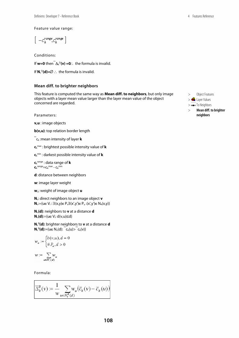
Definiens Developer 7 - Reference Book
108
4 Features Reference
Feature value range:
Conditions:
If w=0 then⎯ΔkD(v) =0∴ the formula is invalid.
If NvD(d)=∅ ∴ the formula is invalid.
Mean diff. to brighter neighbors
This feature is computed the same way as Mean diff. to neighbors, but only image objects with a layer mean value larger than the layer mean value of the object concerned are regarded.
Parameters:
v,u : image objects
b(v,u): top relation border length
⎯ck :mean intensity of layer k
ckmax : brightest possible intensity value of k
ckmin : darkest possible intensity value of k
ckrange : data range of k
ckrange=ck
max - ckmin
d: distance between neighbors
w: image layer weight
wu: weight of image object u
Nv: direct neighbors to an image object v Nv:={u∈Vi : ∃(x,y)∈Pv∃(x',y')∈Pu :(x',y')∈N4(x,y)}
Nv(d): neighbors to v at a distance d Nv(d):={u∈Vi: d(v,u)≤d}
NvB(d): brighter neighbors to v at a distance d
NvB(d):={u∈Nv(d): ⎯ck(u)>⎯ck(v)}
Formula:
> Object Features > Layer Values > To Neighbors > Mean diff. to brighter
neighbors
Definiens Developer 7 - Reference Book
109
4 Features Reference
Feature value range:
Conditions:
If w=0 then⎯ΔkB(v) =0∴ the formula is invalid.
If NvB(d)=∅ ∴ the formula is invalid.
Rel. border to brighter neighbors
Ratio of shared border with image objects of a higher mean value in the selected layer and the total border of the image object concerned.
Parameters:
NvB(d): brighter neighbors to v at a distance d
NvB(d):={u∈Nv(d): ⎯ck(u)>ck(v)}
bv : image object border length
b(v,u): top relation border length
d: distance between neighbors
Formula:
Feature value range:
[0,1]
4.3.2.5 To Superobject
Mean Diff. to Superobject
Difference between layer L mean value of an image object and the layer L mean value of its superobject. You can determine in which image object level the superobject is selected by editing the feature distance.
Parameters:
⎯ck :mean intensity of layer k
ckrange : data range of k
ckrange :=ck
max :-ckmin
Sv(d) : subobject of v with hierarchical distance d
> Object Features > Layer Values > To Neighbors > Rel. border to brighter
neighbors
> Object Features > Layer Values > To Superobject
> Object Features > Layer Values > To Superobject > Mean diff. to
superobject
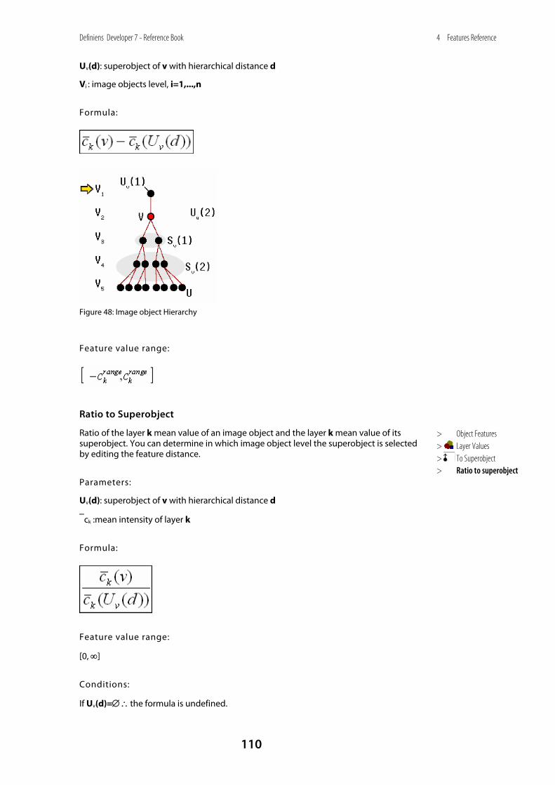
Definiens Developer 7 - Reference Book
110
4 Features Reference
Uv(d): superobject of v with hierarchical distance d
Vi : image objects level, i=1,...,n
Formula:
Figure 48: Image object Hierarchy
Feature value range:
Ratio to Superobject
Ratio of the layer k mean value of an image object and the layer k mean value of its superobject. You can determine in which image object level the superobject is selected by editing the feature distance.
Parameters:
Uv(d): superobject of v with hierarchical distance d
⎯ck :mean intensity of layer k
Formula:
Feature value range:
[0, ∞]
Conditions:
If Uv(d)=∅ ∴the formula is undefined.
> Object Features > Layer Values > To Superobject > Ratio to superobject
Definiens Developer 7 - Reference Book
111
4 Features Reference
If Uv(d)=0 →∞ ∴the formula is undefined.
Stddev. Diff. to Superobject
Difference between layer k Stddev value of an image object and the layer k Stddev of its superobject. You can determine in which image object level the superobject is selected by editing the feature distance.
Parameters:
Uv(d): superobject of v with hierarchical distance d
σk(v) : std. deviation of object v on layer k
ckrange : data range of layer k
ckrange :=ck
max :-ckmin
Formula:
Feature value range:
Condition:
If Uv(d)=∅ ∴the formula is undefined.
Stddev. Ratio to Superobject
Ratio of the layer k standard deviation of an image object and the layer k standard deviation of its superobject. You can determine in which image object level the superobject is selected by editing the feature distance.
Parameters:
Uv(d): super object of v with hierarchical distance d
σk(v) : std. deviation of object v on layer k
Formula:
Feature value range:
[0,∞]
> Object Features > Layer Values > To Superobject > Stddev. diff. to
superobject
> Object Features > Layer Values > To Superobject > Stddev. ratio. to
superobject
Definiens Developer 7 - Reference Book
112
4 Features Reference
Conditions:
If Uv(d)=∅ ∴the formula is undefined.
If σk(Uv(d))=0 ⇒the std. deviation ratio to Uv(d) =1.
4.3.2.6 To Scene
Mean diff. to scene
Difference between layer K mean value of an image object and the layer K mean value of the whole scene.
Parameters:
⎯ck: mean intensity of layer k
⎯ck(v): mean intensity of layer k of an image object v
ckrange : data range of layer k
ckrange :=ck
max :-ckmin
Formula:
Feature value range:
Ratio to scene
Ratio to scene of layer k is the layer k mean value of an image object divided by the layer k mean value of the whole scene.
Parameters:
⎯ck: mean intensity of layer k
⎯ck(v): mean intensity of layer k of an image object v
Formula:
Feature value range:
[-∞, ∞]
> Object Features > Layer Values > To Scene
> Object Features > Layer Values > To Scene > Mean diff. to scene
> Object Features > Layer Values > To Scene > Ratio to scene
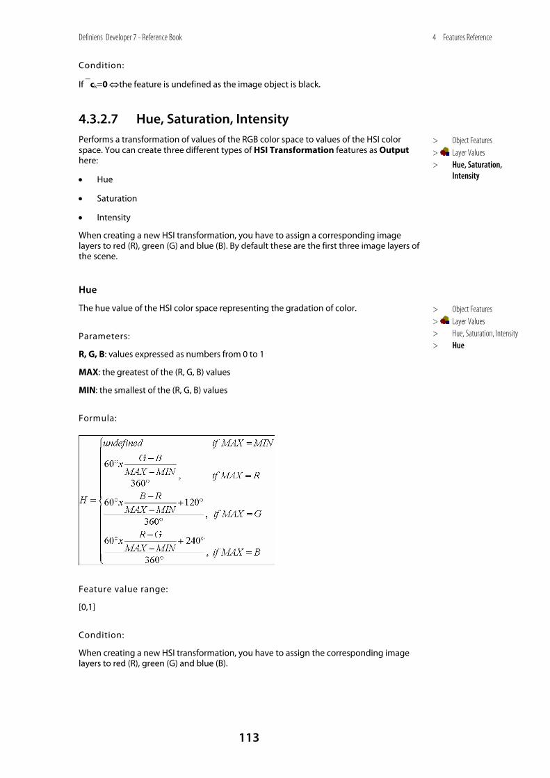
Definiens Developer 7 - Reference Book
113
4 Features Reference
Condition:
If ⎯ck=0 ⇔the feature is undefined as the image object is black.
4.3.2.7 Hue, Saturation, Intensity Performs a transformation of values of the RGB color space to values of the HSI color space. You can create three different types of HSI Transformation features as Output here:
• Hue
• Saturation
• Intensity
When creating a new HSI transformation, you have to assign a corresponding image layers to red (R), green (G) and blue (B). By default these are the first three image layers of the scene.
Hue
The hue value of the HSI color space representing the gradation of color.
Parameters:
R, G, B: values expressed as numbers from 0 to 1
MAX: the greatest of the (R, G, B) values
MIN: the smallest of the (R, G, B) values
Formula:
Feature value range:
[0,1]
Condition:
When creating a new HSI transformation, you have to assign the corresponding image layers to red (R), green (G) and blue (B).
> Object Features > Layer Values > Hue, Saturation,
Intensity
> Object Features > Layer Values > Hue, Saturation, Intensity > Hue

Definiens Developer 7 - Reference Book
114
4 Features Reference
Saturation
The saturation value of the HSI color space representing the intensity of a specific hue.
Parameters:
R, G, B: values expressed as numbers from 0 to 1
MAX: the greatest of the (R, G, B) values
MIN: the least of the (R, G, B) values
Formula:
Feature value range:
[0,1]
Conditions:
When creating a new HSI transformation, you have to assign the according image layers to red (R), green (G) and blue (B).
Intensity
The intensity value of the HSI color space representing the lightness spanning the entire range from black through the chosen hue to white.
Parameters:
R, G, B: values expressed as numbers from 0 to 1
MAX: the greatest of the (R, G, B) values
MIN: the least of the (R, G, B) values
Formula:
I=MAX
Feature value range:
[0,1]
Condition:
When creating a new HSI transformation, you have to assign the according image layers to red (R), green (G) and blue (B).
> Object Features > Layer Values > Hue, Saturation, Intensity > Saturation
> Object Features > Layer Values > Hue, Saturation, Intensity > Intensity
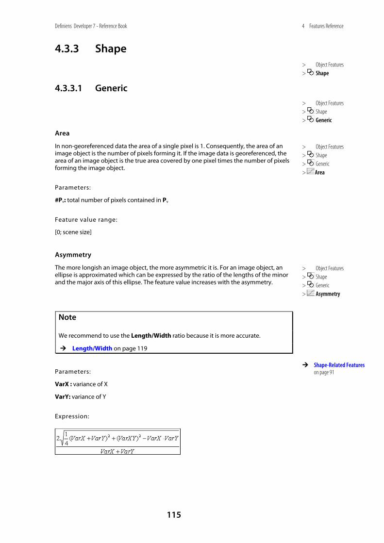
Definiens Developer 7 - Reference Book
115
4 Features Reference
4.3.3 Shape
4.3.3.1 Generic
Area
In non-georeferenced data the area of a single pixel is 1. Consequently, the area of an image object is the number of pixels forming it. If the image data is georeferenced, the area of an image object is the true area covered by one pixel times the number of pixels forming the image object.
Parameters:
#Pv: total number of pixels contained in Pv
Feature value range:
[0; scene size]
Asymmetry
The more longish an image object, the more asymmetric it is. For an image object, an ellipse is approximated which can be expressed by the ratio of the lengths of the minor and the major axis of this ellipse. The feature value increases with the asymmetry.
Note
We recommend to use the Length/Width ratio because it is more accurate.
Length/Width on page 119
Parameters:
VarX : variance of X
VarY: variance of Y
Expression:
> Object Features > Shape
> Object Features > Shape > Generic
> Object Features > Shape > Generic > Area
> Object Features > Shape > Generic > Asymmetry
Shape-Related Features on page 91
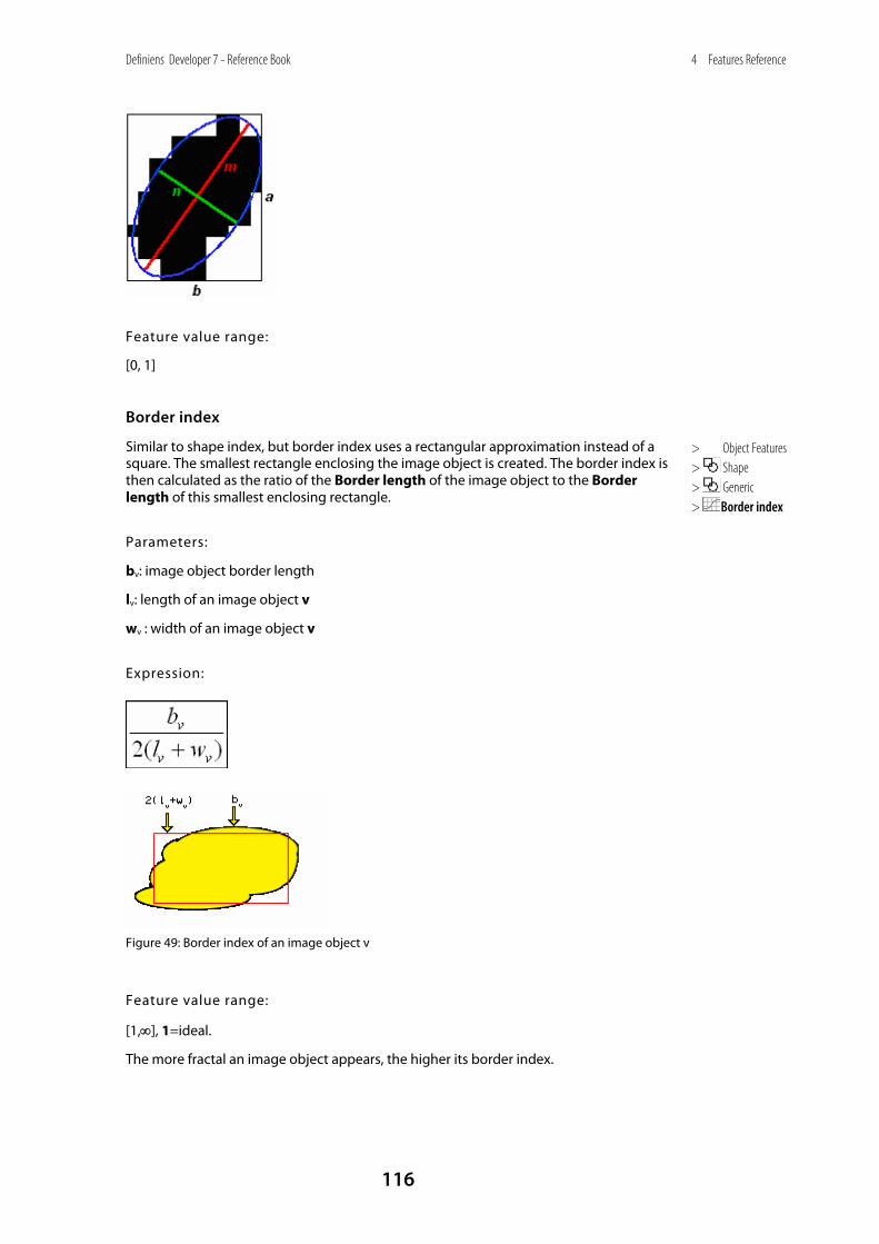
Definiens Developer 7 - Reference Book
116
4 Features Reference
Feature value range:
[0, 1]
Border index
Similar to shape index, but border index uses a rectangular approximation instead of a square. The smallest rectangle enclosing the image object is created. The border index is then calculated as the ratio of the Border length of the image object to the Border length of this smallest enclosing rectangle.
Parameters:
bv: image object border length
lv: length of an image object v
wv : width of an image object v
Expression:
Figure 49: Border index of an image object v
Feature value range:
[1,∞], 1=ideal.
The more fractal an image object appears, the higher its border index.
> Object Features > Shape > Generic > Border index
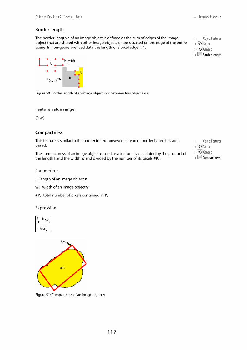
Definiens Developer 7 - Reference Book
117
4 Features Reference
Border length
The border length e of an image object is defined as the sum of edges of the image object that are shared with other image objects or are situated on the edge of the entire scene. In non-georeferenced data the length of a pixel edge is 1.
Figure 50: Border length of an image object v or between two objects v, u.
Feature value range:
[0, ∞]
Compactness
This feature is similar to the border index, however instead of border based it is area based.
The compactness of an image object v, used as a feature, is calculated by the product of the length l and the width w and divided by the number of its pixels #Pv.
Parameters:
lv: length of an image object v
wv : width of an image object v
#Pv: total number of pixels contained in Pv
Expression:
Figure 51: Compactness of an image object v
> Object Features > Shape > Generic > Border length
> Object Features > Shape > Generic > Compactness
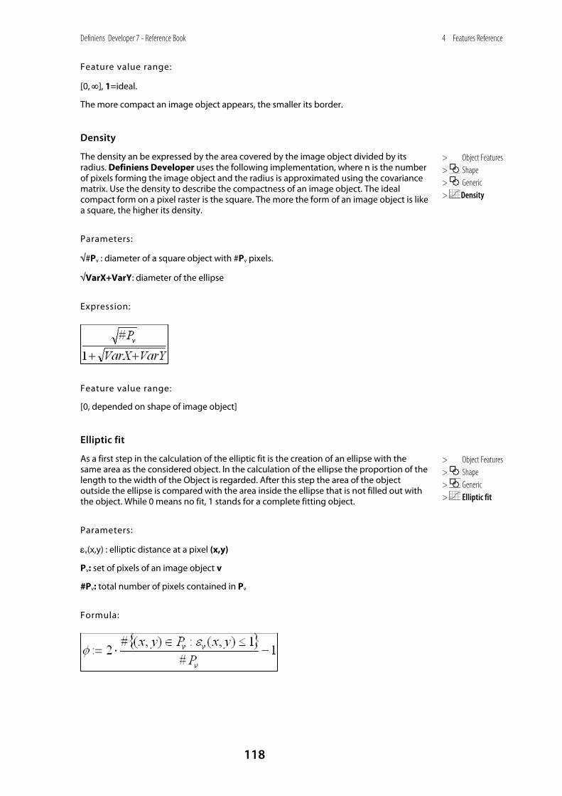
Definiens Developer 7 - Reference Book
118
4 Features Reference
Feature value range:
[0, ∞], 1=ideal.
The more compact an image object appears, the smaller its border.
Density
The density an be expressed by the area covered by the image object divided by its radius. Definiens Developer uses the following implementation, where n is the number of pixels forming the image object and the radius is approximated using the covariance matrix. Use the density to describe the compactness of an image object. The ideal compact form on a pixel raster is the square. The more the form of an image object is like a square, the higher its density.
Parameters:
√#Pv : diameter of a square object with #Pv pixels.
√VarX+VarY: diameter of the ellipse
Expression:
Feature value range:
[0, depended on shape of image object]
Elliptic fit
As a first step in the calculation of the elliptic fit is the creation of an ellipse with the same area as the considered object. In the calculation of the ellipse the proportion of the length to the width of the Object is regarded. After this step the area of the object outside the ellipse is compared with the area inside the ellipse that is not filled out with the object. While 0 means no fit, 1 stands for a complete fitting object.
Parameters:
εv(x,y) : elliptic distance at a pixel (x,y)
Pv: set of pixels of an image object v
#Pv: total number of pixels contained in Pv
Formula:
> Object Features > Shape > Generic > Density
> Object Features > Shape > Generic > Elliptic fit
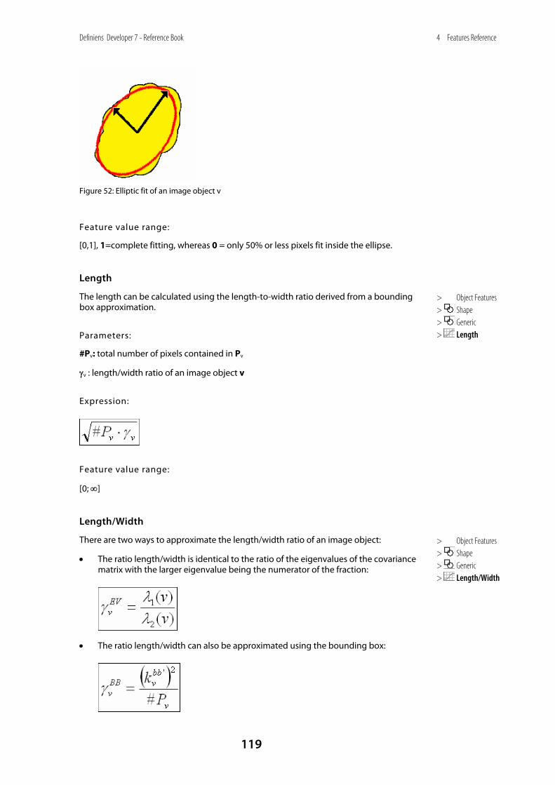
Definiens Developer 7 - Reference Book
119
4 Features Reference
Figure 52: Elliptic fit of an image object v
Feature value range:
[0,1], 1=complete fitting, whereas 0 = only 50% or less pixels fit inside the ellipse.
Length
The length can be calculated using the length-to-width ratio derived from a bounding box approximation.
Parameters:
#Pv: total number of pixels contained in Pv
γv : length/width ratio of an image object v
Expression:
Feature value range:
[0; ∞]
Length/Width
There are two ways to approximate the length/width ratio of an image object:
• The ratio length/width is identical to the ratio of the eigenvalues of the covariance matrix with the larger eigenvalue being the numerator of the fraction:
• The ratio length/width can also be approximated using the bounding box:
> Object Features > Shape > Generic > Length
> Object Features > Shape > Generic > Length/Width
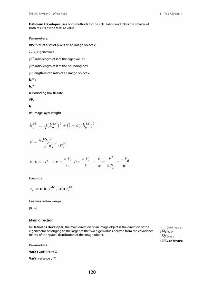
Definiens Developer 7 - Reference Book
120
4 Features Reference
Definiens Developer uses both methods for the calculation and takes the smaller of both results as the feature value.
Parameters:
#Pv :Size of a set of pixels of an image object v
λ1, λ2:eigenvalues
γvEV :ratio length of v of the eigenvalues
γvBB :ratio length of v of the bounding box
γv : length/width ratio of an image object v
kvbb' :
hvbb :
a: Bounding box fill rate
#Pxl
h :
w : image layer weight
Formula:
Feature value range:
[0; ∞]
Main direction
In Definiens Developer, the main direction of an image object is the direction of the eigenvector belonging to the larger of the two eigenvalues derived from the covariance matrix of the spatial distribution of the image object.
Parameters:
VarX : variance of X
VarY: variance of Y
> Object Features > Shape > Generic > Main direction
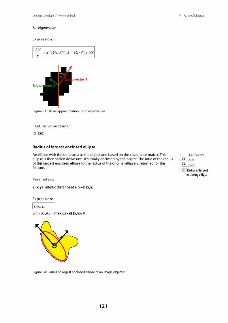
Definiens Developer 7 - Reference Book
121
4 Features Reference
λ1 : eigenvalue
Expression:
Figure 53: Ellipse approximation using eigenvalues.
Feature value range:
[0; 180]
Radius of largest enclosed ellipse
An ellipse with the same area as the object and based on the covariance matrix. This ellipse is then scaled down until it's totally enclosed by the object. The ratio of the radius of this largest enclosed ellipse to the radius of the original ellipse is returned for this feature.
Parameters:
εv(x,y) : elliptic distance at a pixel (x,y)
Expression:
εv(xo,yo)
with (xo,yo) = max εv(x,y), (x,y)∈Pv
Figure 54: Radius of largest enclosed ellipse of an image object v
> Object Features > Shape > Generic > Radius of largest
enclosing ellipse
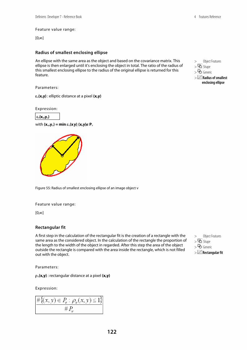
Definiens Developer 7 - Reference Book
122
4 Features Reference
Feature value range:
[0,∞]
Radius of smallest enclosing ellipse
An ellipse with the same area as the object and based on the covariance matrix. This ellipse is then enlarged until it's enclosing the object in total. The ratio of the radius of this smallest enclosing ellipse to the radius of the original ellipse is returned for this feature.
Parameters:
εv(x,y) : elliptic distance at a pixel (x,y)
Expression:
εv(xo,yo)
with (xo,yo) = min εv(x,y), (x,y)∉Pv
Figure 55: Radius of smallest enclosing ellipse of an image object v
Feature value range:
[0,∞]
Rectangular fit
A first step in the calculation of the rectangular fit is the creation of a rectangle with the same area as the considered object. In the calculation of the rectangle the proportion of the length to the width of the object in regarded. After this step the area of the object outside the rectangle is compared with the area inside the rectangle, which is not filled out with the object.
Parameters:
ρv(x,y) : rectangular distance at a pixel (x,y)
Expression:
> Object Features > Shape > Generic > Radius of smallest
enclosing ellipse
> Object Features > Shape > Generic > Rectangular fit
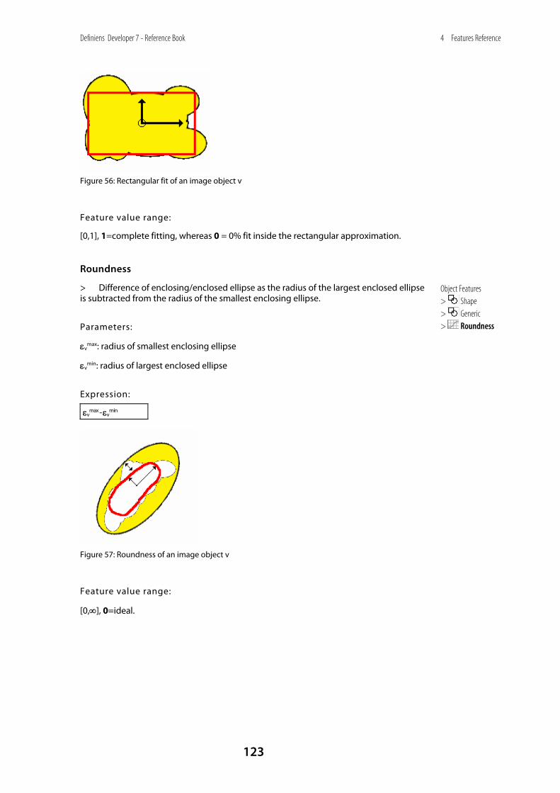
Definiens Developer 7 - Reference Book
123
4 Features Reference
Figure 56: Rectangular fit of an image object v
Feature value range:
[0,1], 1=complete fitting, whereas 0 = 0% fit inside the rectangular approximation.
Roundness
> Difference of enclosing/enclosed ellipse as the radius of the largest enclosed ellipse is subtracted from the radius of the smallest enclosing ellipse.
Parameters:
εvmax: radius of smallest enclosing ellipse
εvmin: radius of largest enclosed ellipse
Expression:
εvmax - εv
min
Figure 57: Roundness of an image object v
Feature value range:
[0,∞], 0=ideal.
Object Features > Shape > Generic > Roundness
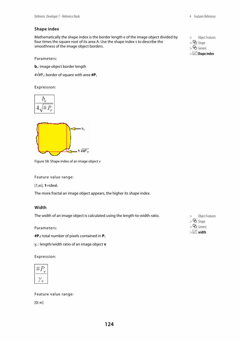
Definiens Developer 7 - Reference Book
124
4 Features Reference
Shape index
Mathematically the shape index is the border length e of the image object divided by four times the square root of its area A. Use the shape index s to describe the smoothness of the image object borders.
Parameters:
bv: image object border length
4√#Pv: border of square with area #Pv
Expression:
Figure 58: Shape index of an image object v
Feature value range:
[1,∞], 1=ideal.
The more fractal an image object appears, the higher its shape index.
Width
The width of an image object is calculated using the length-to-width ratio.
Parameters:
#Pv: total number of pixels contained in Pv
γv : length/width ratio of an image object v
Expression:
Feature value range:
[0; ∞]
> Object Features > Shape > Generic > Shape index
> Object Features > Shape > Generic > width

Definiens Developer 7 - Reference Book
125
4 Features Reference
4.3.3.2 Line Features Based on Subobject Analysis The information for classification of an object can also be derived from information provided by its subobjects. A specific method is to produce compact sub-objects for the purpose of line analysis. The basic idea is to represent the shape of an object by compact subobjects and operate from center point to center point to get line information. Nevertheless it is possible to determine to which image object level the feature should refer to.
As mentioned above, this method is superior to bounding box approximation, if you want to extract features out of lengthy and curved image objects (e.g., image objects representing rivers or roads).
Note
These features are provided for backward compatibility only. It is not recommended to use them in new rule sets.
Width (line so)
The image object width calculated on the basis of sub-objects is the area A (in pixels) of the image object divided by its length derived from sub-object analysis.
Parameters:
•
Formula:
Feature value range:
[1; depending on image object shape]
Length/Width (line so)
The length-to-width ratio based on subobject analysis is the square length derived from subobject analysis divided by the object area (in pixels).
> Object Features > Shape
> Line features based on sub-object analysis
> Object Features > Shape
> Line features based on sub-object analysis
> Width (line so)
> Object Features > Shape
> Line features based on sub-object analysis
> Length/width (line so)
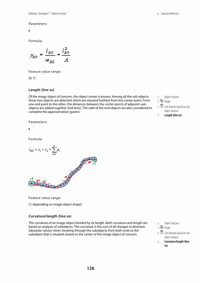
Definiens Developer 7 - Reference Book
126
4 Features Reference
Parameters:
•
Formula:
Feature value range:
[0; 1]
Length (line so)
Of the image object of concern, the object center is known. Among all the sub-objects those two objects are detected which are situated furthest from this center point. From one end point to the other, the distances between the center points of adjacent sub-objects are added together (red lines). The radii of the end objects are also considered to complete the approximation (green)
Parameters:
•
Formula:
Feature value range:
[1; depending on image object shape]
Curvature/length (line so)
The curvature of an image object divided by its length. Both curvature and length are based on analysis of subobjects. The curvature is the sum of all changes in direction (absolute values) when iterating through the subobjects from both ends to the subobject that is situated closest to the center of the image object of concern.
> Object Features > Shape
> Line features based on sub-object analysis
> Length (line so)
> Object Features > Shape
> Line features based on sub-object analysis
> Curvature/length (line so)
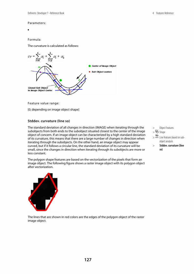
Definiens Developer 7 - Reference Book
127
4 Features Reference
Parameters:
•
Formula:
The curvature is calculated as follows:
Feature value range:
[0; depending on image object shape]
Stddev. curvature (line so)
The standard deviation of all changes in direction (IMAGE) when iterating through the subobjects from both ends to the subobject situated closest to the center of the image object of concern. If an image object can be characterized by a high standard deviation of its curvature, this means that there are a large number of changes in direction when iterating through the subobjects. On the other hand, an image object may appear curved, but if it follows a circular line, the standard deviation of its curvature will be small, since the changes in direction when iterating through its subobjects are more or less constant.
The polygon shape features are based on the vectorization of the pixels that form an image object. The following figure shows a raster image object with its polygon object after vectorization.
The lines that are shown in red colors are the edges of the polygon object of the raster image object.
> Object Features > Shape
> Line features based on sub-object analysis
> Stddev. curvature (line so)
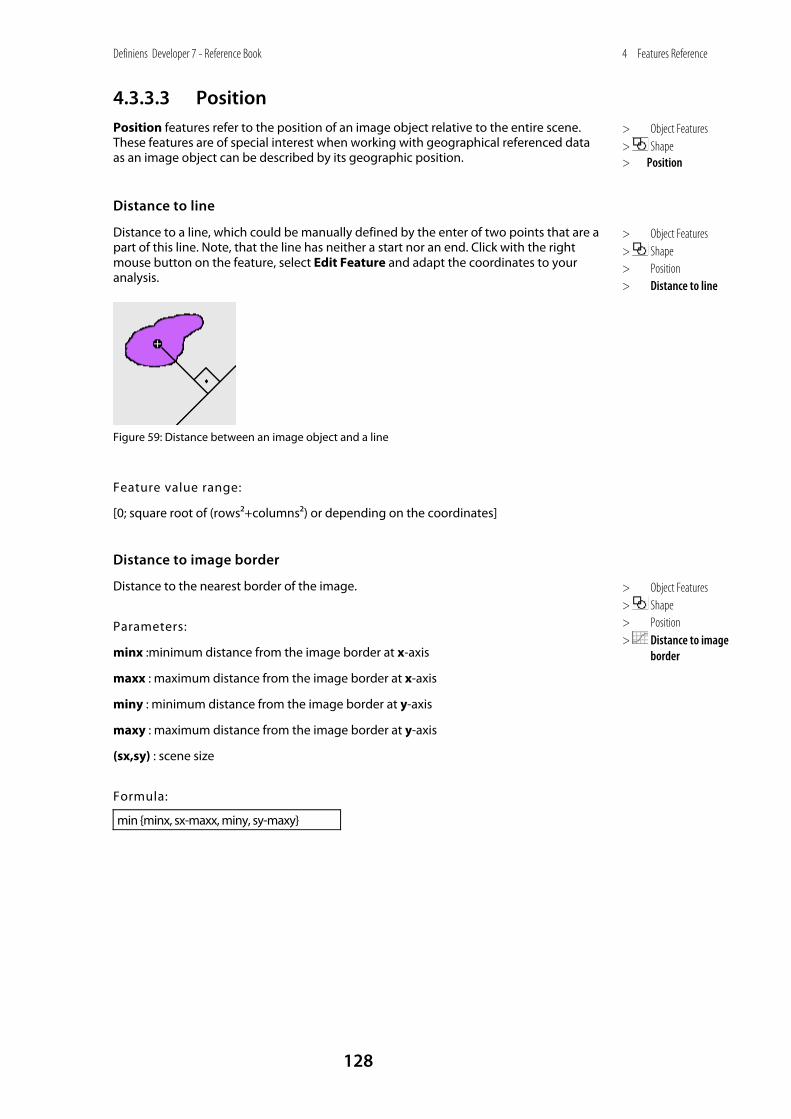
Definiens Developer 7 - Reference Book
128
4 Features Reference
4.3.3.3 Position Position features refer to the position of an image object relative to the entire scene. These features are of special interest when working with geographical referenced data as an image object can be described by its geographic position.
Distance to line
Distance to a line, which could be manually defined by the enter of two points that are a part of this line. Note, that the line has neither a start nor an end. Click with the right mouse button on the feature, select Edit Feature and adapt the coordinates to your analysis.
Figure 59: Distance between an image object and a line
Feature value range:
[0; square root of (rows²+columns²) or depending on the coordinates]
Distance to image border
Distance to the nearest border of the image.
Parameters:
minx :minimum distance from the image border at x-axis
maxx : maximum distance from the image border at x-axis
miny : minimum distance from the image border at y-axis
maxy : maximum distance from the image border at y-axis
(sx,sy) : scene size
Formula:
min {minx, sx-maxx, miny, sy-maxy}
> Object Features > Shape > Position
> Object Features > Shape > Position > Distance to line
> Object Features > Shape > Position > Distance to image
border
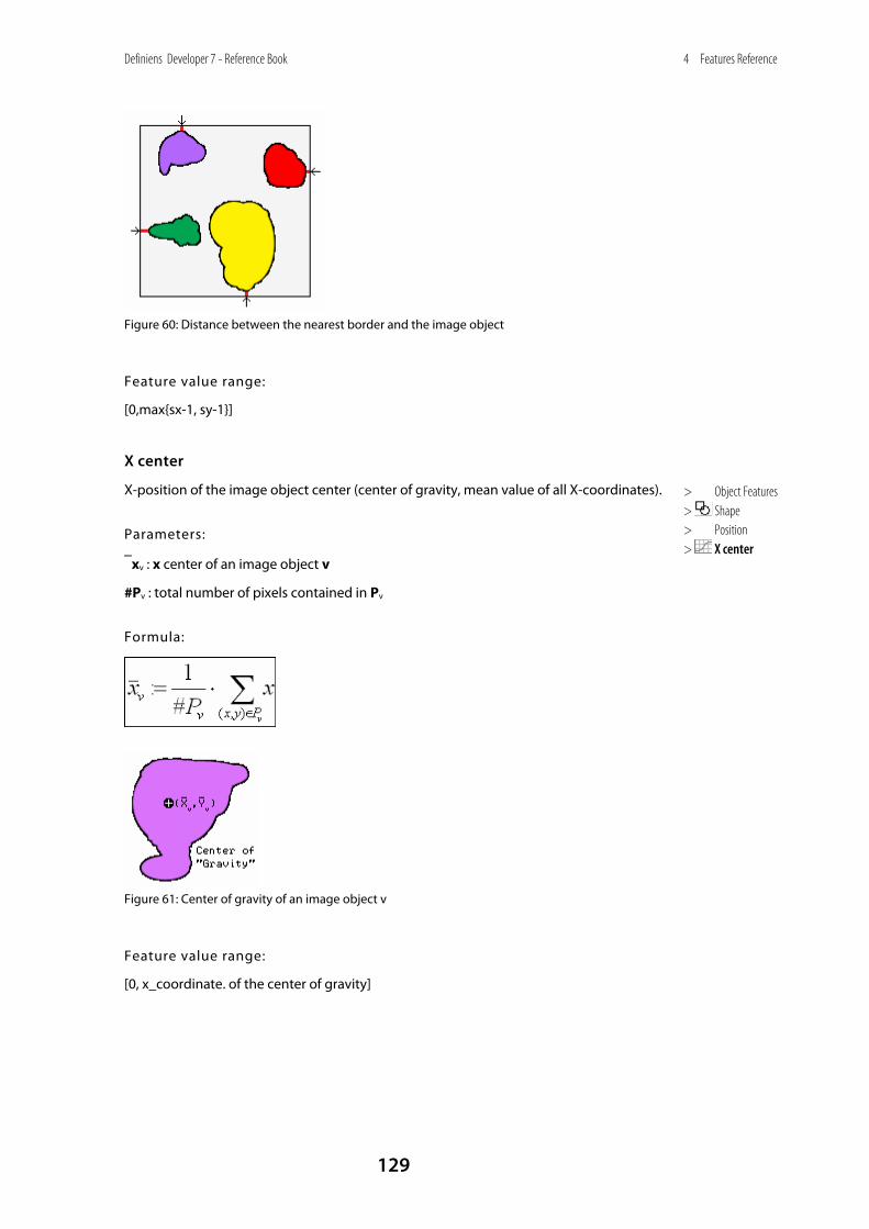
Definiens Developer 7 - Reference Book
129
4 Features Reference
Figure 60: Distance between the nearest border and the image object
Feature value range:
[0,max{sx-1, sy-1}]
X center
X-position of the image object center (center of gravity, mean value of all X-coordinates).
Parameters:
⎯xv : x center of an image object v
#Pv : total number of pixels contained in Pv
Formula:
Figure 61: Center of gravity of an image object v
Feature value range:
[0, x_coordinate. of the center of gravity]
> Object Features > Shape > Position > X center
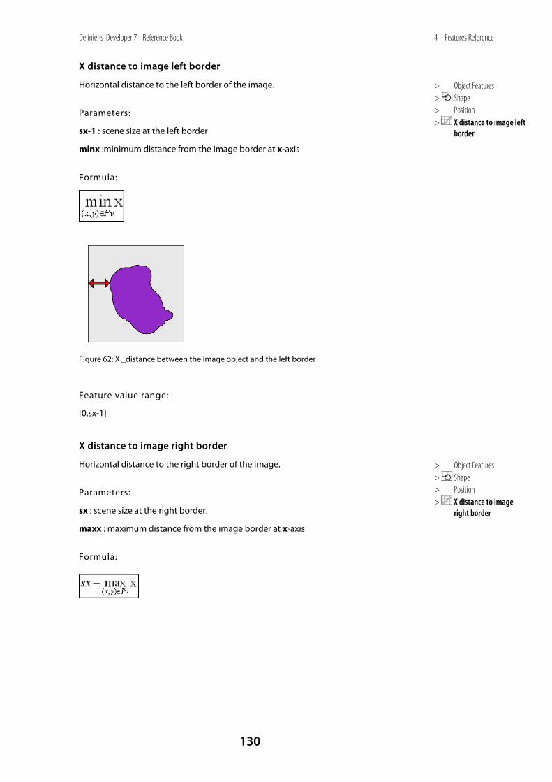
Definiens Developer 7 - Reference Book
130
4 Features Reference
X distance to image left border
Horizontal distance to the left border of the image.
Parameters:
sx-1 : scene size at the left border
minx :minimum distance from the image border at x-axis
Formula:
Figure 62: X _distance between the image object and the left border
Feature value range:
[0,sx-1]
X distance to image right border
Horizontal distance to the right border of the image.
Parameters:
sx : scene size at the right border.
maxx : maximum distance from the image border at x-axis
Formula:
> Object Features > Shape > Position > X distance to image left
border
> Object Features > Shape > Position > X distance to image
right border
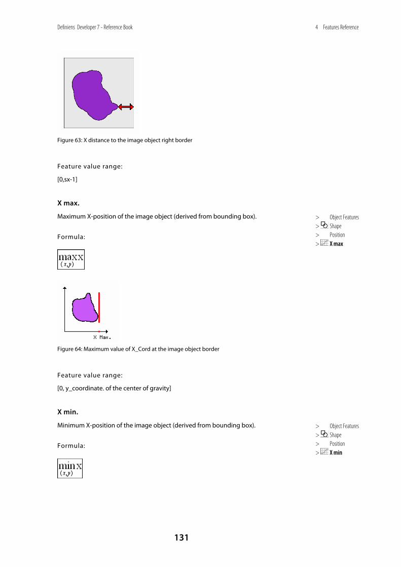
Definiens Developer 7 - Reference Book
131
4 Features Reference
Figure 63: X distance to the image object right border
Feature value range:
[0,sx-1]
X max.
Maximum X-position of the image object (derived from bounding box).
Formula:
Figure 64: Maximum value of X_Cord at the image object border
Feature value range:
[0, y_coordinate. of the center of gravity]
X min.
Minimum X-position of the image object (derived from bounding box).
Formula:
> Object Features > Shape > Position > X max
> Object Features > Shape > Position > X min

Definiens Developer 7 - Reference Book
132
4 Features Reference
Figure 65: Minimum value of X_Cord at the image object border
Feature value range:
[0, y_coordinate. of the center of gravity]
Y max.
Maximum Y-position of the image object (derived from bounding box).
Formula:
Figure 66: Maximum value of Y_Cord at the image object border.
Feature value range:
[0, y_coordinate. of the center of gravity]
Y center
Y-position of the image object center (center of gravity, mean value of all Y-coordinates).
Parameters:
⎯yv : y center of an image object v
#Pv : total number of pixels contained in Pv
> Object Features > Shape > Position > Y max
> Object Features > Shape > Position > Y center
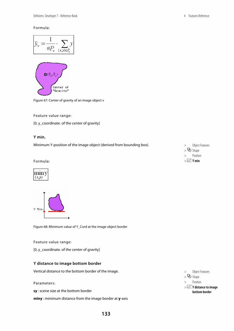
Definiens Developer 7 - Reference Book
133
4 Features Reference
Formula:
Figure 67: Center of gravity of an image object v
Feature value range:
[0, y_coordinate. of the center of gravity]
Y min.
Minimum Y-position of the image object (derived from bounding box).
Formula:
Figure 68: Minimum value of Y_Cord at the image object border
Feature value range:
[0, y_coordinate. of the center of gravity]
Y distance to image bottom border
Vertical distance to the bottom border of the image.
Parameters:
sy : scene size at the bottom border
miny : minimum distance from the image border at y-axis
> Object Features > Shape > Position > Y min
> Object Features > Shape > Position > Y distance to image
bottom border
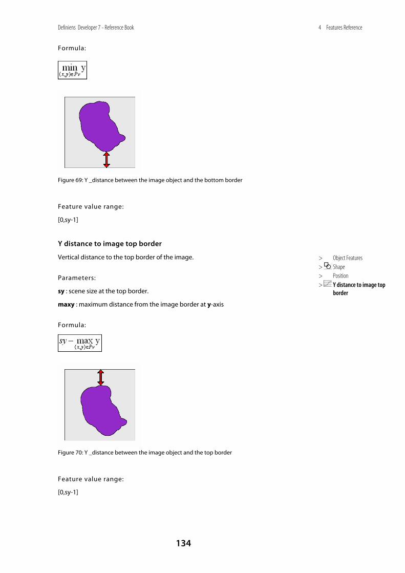
Definiens Developer 7 - Reference Book
134
4 Features Reference
Formula:
Figure 69: Y _distance between the image object and the bottom border
Feature value range:
[0,sy-1]
Y distance to image top border
Vertical distance to the top border of the image.
Parameters:
sy : scene size at the top border.
maxy : maximum distance from the image border at y-axis
Formula:
Figure 70: Y _distance between the image object and the top border
Feature value range:
[0,sy-1]
> Object Features > Shape > Position > Y distance to image top
border
Definiens Developer 7 - Reference Book
135
4 Features Reference
4.3.3.4 To Superobject Use To Superobject features to describe an image object by its form relations to one of its superobjects (if there are any). Which superobject is to be referred to is defined by editing the feature distance (n). Especially when working with thematic layers these features might be of great interest.
Rel. area to superobject
The feature is computed by dividing the area of the image object of concern by the area covered by its superobject. If the feature value is 1, then the image object is identical to its superobject. Use this feature to describe an image object by the amount of area it covers of its superobject.
Parameters:
#Pv : total number of pixels contained in Pv
#PUv(d) : the size of the superobject of v
Formula:
Condition:
If Uv(d) =∅ ∴the formula is undefined.
Feature value range:
[0,1]
Rel. rad. position to superobject (n)
The feature value is calculated by dividing the distance from the center of the image object of concern to the center of its superobject by the distance of the center of the most distant image object which has the same superobject.
Use this feature to describe an image object by its position relative to the center of its superobject.
Parameters:
#Pv : total number of pixels contained in Pv
#PUv(d) : the size of the superobject of an image object v
dg(v,Uv(d)) : distance of v to the center of gravity of the superobject Uv(d)
> Object Features > Shape > To Superobject
> Object Features > Shape > To Superobject > Rel. area to superobject
> Object Features > Shape > To Superobject > Rel. rad. position to
superobject
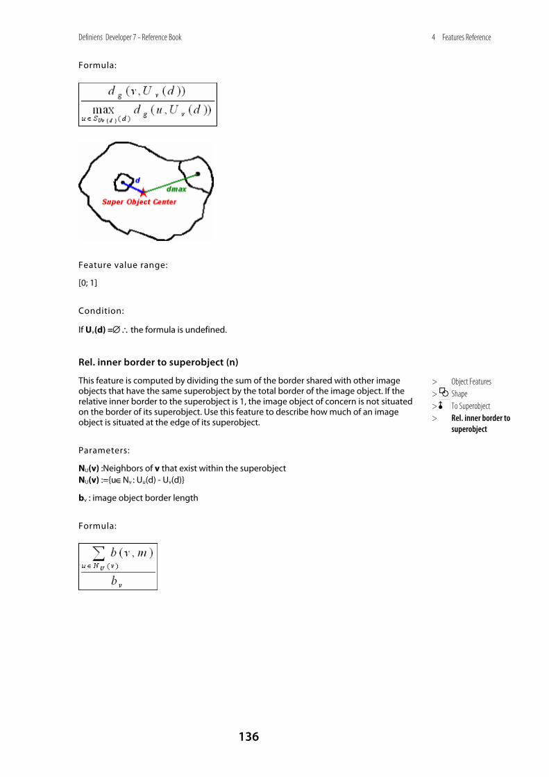
Definiens Developer 7 - Reference Book
136
4 Features Reference
Formula:
Feature value range:
[0; 1]
Condition:
If Uv(d) =∅ ∴the formula is undefined.
Rel. inner border to superobject (n)
This feature is computed by dividing the sum of the border shared with other image objects that have the same superobject by the total border of the image object. If the relative inner border to the superobject is 1, the image object of concern is not situated on the border of its superobject. Use this feature to describe how much of an image object is situated at the edge of its superobject.
Parameters:
NU(v) :Neighbors of v that exist within the superobject NU(v) :={u∈Nv : Uu(d) - Uv(d)}
bv : image object border length
Formula:
> Object Features > Shape > To Superobject > Rel. inner border to
superobject
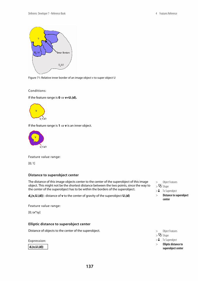
Definiens Developer 7 - Reference Book
137
4 Features Reference
Figure 71: Relative inner border of an image object v to super object U
Conditions:
If the feature range is 0 ⇒ v=Uv(d).
If the feature range is 1 ⇒ v is an inner object.
Feature value range:
[0; 1]
Distance to superobject center
The distance of this image objects center to the center of the superobject of this image object. This might not be the shortest distance between the two points, since the way to the center of the superobject has to be within the borders of the superobject.
dg(v,Uv(d)) : distance of v to the center of gravity of the superobject Uv(d)
Feature value range:
[0; sx*sy]
Elliptic distance to superobject center
Distance of objects to the center of the superobject.
Expression:
de(v,Uv(d))
> Object Features > Shape > To Superobject > Distance to superobject
center
> Object Features > Shape > To Superobject > Elliptic distance to
superobject center
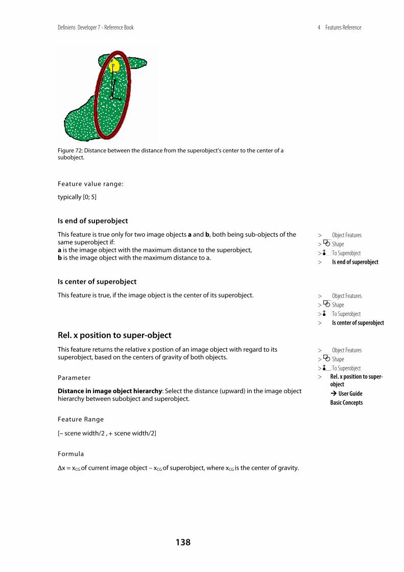
Definiens Developer 7 - Reference Book
138
4 Features Reference
Figure 72: Distance between the distance from the superobject's center to the center of a subobject.
Feature value range:
typically [0; 5]
Is end of superobject
This feature is true only for two image objects a and b, both being sub-objects of the same superobject if: a is the image object with the maximum distance to the superobject, b is the image object with the maximum distance to a.
Is center of superobject
This feature is true, if the image object is the center of its superobject.
Rel. x position to super-object
This feature returns the relative x postion of an image object with regard to its superobject, based on the centers of gravity of both objects.
Parameter
Distance in image object hierarchy: Select the distance (upward) in the image object hierarchy between subobject and superobject.
Feature Range
[– scene width/2 , + scene width/2]
Formula
Δx = xCG of current image object – xCG of superobject, where xCG is the center of gravity.
> Object Features > Shape > To Superobject > Is end of superobject
> Object Features > Shape > To Superobject > Is center of superobject
> Object Features > Shape > To Superobject > Rel. x position to super-
object User Guide Basic Concepts
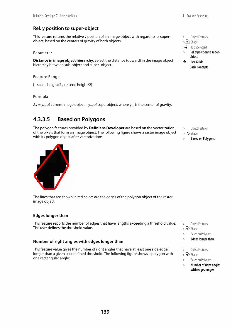
Definiens Developer 7 - Reference Book
139
4 Features Reference
Rel. y position to super-object
This feature returns the relative y postion of an image object with regard to its super-object, based on the centers of gravity of both objects.
Parameter
Distance in image object hierarchy: Select the distance (upward) in the image object hierarchy between sub-object and super -object.
Feature Range
[– scene height/2 , + scene height/2]
Formula
Δy = yCG of current image object – yCG of superobject, where yCG is the center of gravity.
4.3.3.5 Based on Polygons The polygon features provided by Definiens Developer are based on the vectorization of the pixels that form an image object. The following figure shows a raster image object with its polygon object after vectorization:
The lines that are shown in red colors are the edges of the polygon object of the raster image object.
Edges longer than
This feature reports the number of edges that have lengths exceeding a threshold value. The user defines the threshold value.
Number of right angles with edges longer than
This feature value gives the number of right angles that have at least one side edge longer than a given user defined threshold. The following figure shows a polygon with one rectangular angle:
> Object Features > Shape > To Superobject > Rel. y position to super-
object User Guide
Basic Concepts
> Object Features > Shape > Based on Polygons
> Object Features > Shape > Based on Polygons > Edges longer than
> Object Features > Shape > Based on Polygons > Number of right angles
with edges longer
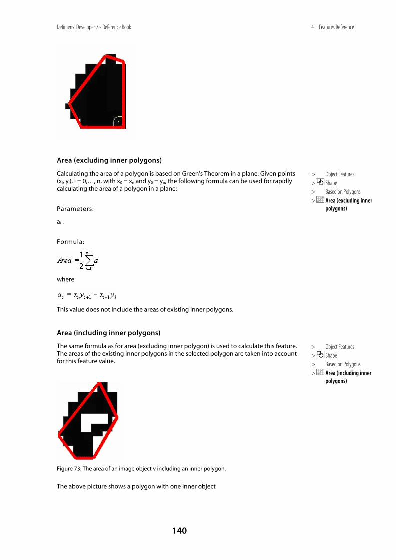
Definiens Developer 7 - Reference Book
140
4 Features Reference
Area (excluding inner polygons)
Calculating the area of a polygon is based on Green's Theorem in a plane. Given points (xi, yi), i = 0,…, n, with x0 = xn and y0 = yn, the following formula can be used for rapidly calculating the area of a polygon in a plane:
Parameters:
ai :
Formula:
where
This value does not include the areas of existing inner polygons.
Area (including inner polygons)
The same formula as for area (excluding inner polygon) is used to calculate this feature. The areas of the existing inner polygons in the selected polygon are taken into account for this feature value.
Figure 73: The area of an image object v including an inner polygon.
The above picture shows a polygon with one inner object
> Object Features > Shape > Based on Polygons > Area (excluding inner
polygons)
> Object Features > Shape > Based on Polygons > Area (including inner
polygons)
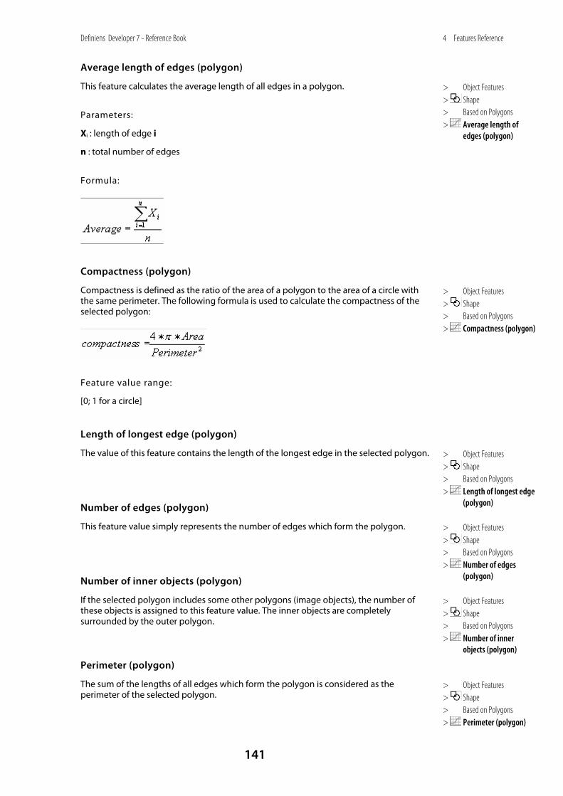
Definiens Developer 7 - Reference Book
141
4 Features Reference
Average length of edges (polygon)
This feature calculates the average length of all edges in a polygon.
Parameters:
Xi : length of edge i
n : total number of edges
Formula:
Compactness (polygon)
Compactness is defined as the ratio of the area of a polygon to the area of a circle with the same perimeter. The following formula is used to calculate the compactness of the selected polygon:
Feature value range:
[0; 1 for a circle]
Length of longest edge (polygon)
The value of this feature contains the length of the longest edge in the selected polygon.
Number of edges (polygon)
This feature value simply represents the number of edges which form the polygon.
Number of inner objects (polygon)
If the selected polygon includes some other polygons (image objects), the number of these objects is assigned to this feature value. The inner objects are completely surrounded by the outer polygon.
Perimeter (polygon)
The sum of the lengths of all edges which form the polygon is considered as the perimeter of the selected polygon.
> Object Features > Shape > Based on Polygons > Average length of
edges (polygon)
> Object Features > Shape > Based on Polygons > Compactness (polygon)
> Object Features > Shape > Based on Polygons > Length of longest edge
(polygon)
> Object Features > Shape > Based on Polygons > Number of edges
(polygon)
> Object Features > Shape > Based on Polygons > Number of inner
objects (polygon)
> Object Features > Shape > Based on Polygons > Perimeter (polygon)
Definiens Developer 7 - Reference Book
142
4 Features Reference
Polygon self-intersection (polygon)
The feature polygon intersection allows identifying a rarely occurring special constellation of image objects which leads to a polygon self-intersection when exported as a polygon vector file.
This feature enables you to identify the affected objects and take measures to avoid the self-intersection. All objects with a value of 1 will cause a polygon self-intersection when exported to a shape file.
The type of object pictured below will lead to a self-intersection at the circled point. To avoid the self-intersection, the enclosed object needs to be merged with the enclosing object.
Tip
Use the image object fusion algorithm to remove polygon intersections. To do so, set the domain to all objects which have a value larger than 0 for the polygon intersection feature. In the algorithm parameter, set the fitting function threshold to polygon intersection = 0, in the weighted sum setting set Target value factor to 1. This will merge all objects with a value of 1 for the feature polygon intersection so that the resulting object will not sport a self intersection.
Stddev of length of edges (polygon)
This feature value shows how the lengths of edges deviate from their mean value. The following formula for standard deviation is used to compute this value.
Parameters:
Xi : length of edge i
⎯X : mean value of all lengths
n : total number of edges
Formula:
4.3.3.6 Based on Skeletons
Image Object Fusion on page 43
> Object Features > Shape > Based on Polygons > Stddev of length of
edges
Definiens Developer 7 - Reference Book
143
4 Features Reference
For the better understanding of the following descriptions the skeleton is divided in a main line and branches as above mentioned. Each mid-point of the triangles created by the Delaunay Triangulation is called a node.
Number of segments of order
Number of segments of order calculates the number of line segments of branches with a selected order. Note, that only segments are counted that do not belong to a lower order. Define the branch order in the dialog Edit Parametrized Features. To open this dialog select Edit Features from the pop up menu that is opened with a right click on the corresponding feature. For more information see Parametrized Features section.
Feature value range:
[0; depending on shape of objects]
Number of branches of order
Number of branches of order calculates the number of branches of a predefined order. Define the branch order in the dialog Edit Parametrized Features. To open this dialog select Edit Feature from the pop up menu that is opened with a right click on the corresponding feature. For more information see Parametrized Features section.
Feature value range:
[0; depending on shape of objects]
Average length of branches of order
Average length of branches of order calculates the average length of branches of a selected order. The length of the branch of the selected order is measured from the intersect point of the whole branch and the main line to the end of the branch. The order can be manually defined. With a right click on the feature a pop up menu opens where you have to select Edit Feature. In the dialog it is possible to select the order of the branches to select. For more information see Parametrized Features section.
Feature value range:
[0; depending on shape of objects]
Number of branches of length
Number of branches of length calculates the number of branches of a special length up to a selected order. At this all ends of branches are counted up to the selected order. Since it is a parametrized feature it is possible to select the branch order and the length in a special range manually. To do so, select Edit Feature from the pop up menu you can open with a right click. For more information see Parametrized Features section.
Feature value range:
[0; depending on shape of objects]
Average branch length
> Object Features > Shape > Based on Skeletons
> Object Features > Shape > Based on Skeletons > Number of segments of
order
> Object Features > Shape > Based on Skeletons > Number of branches of
order
> Object Features > Shape > Based on Skeletons > Average length of
branches of order
> Object Features > Shape > Based on Skeletons > Number of branches of
length
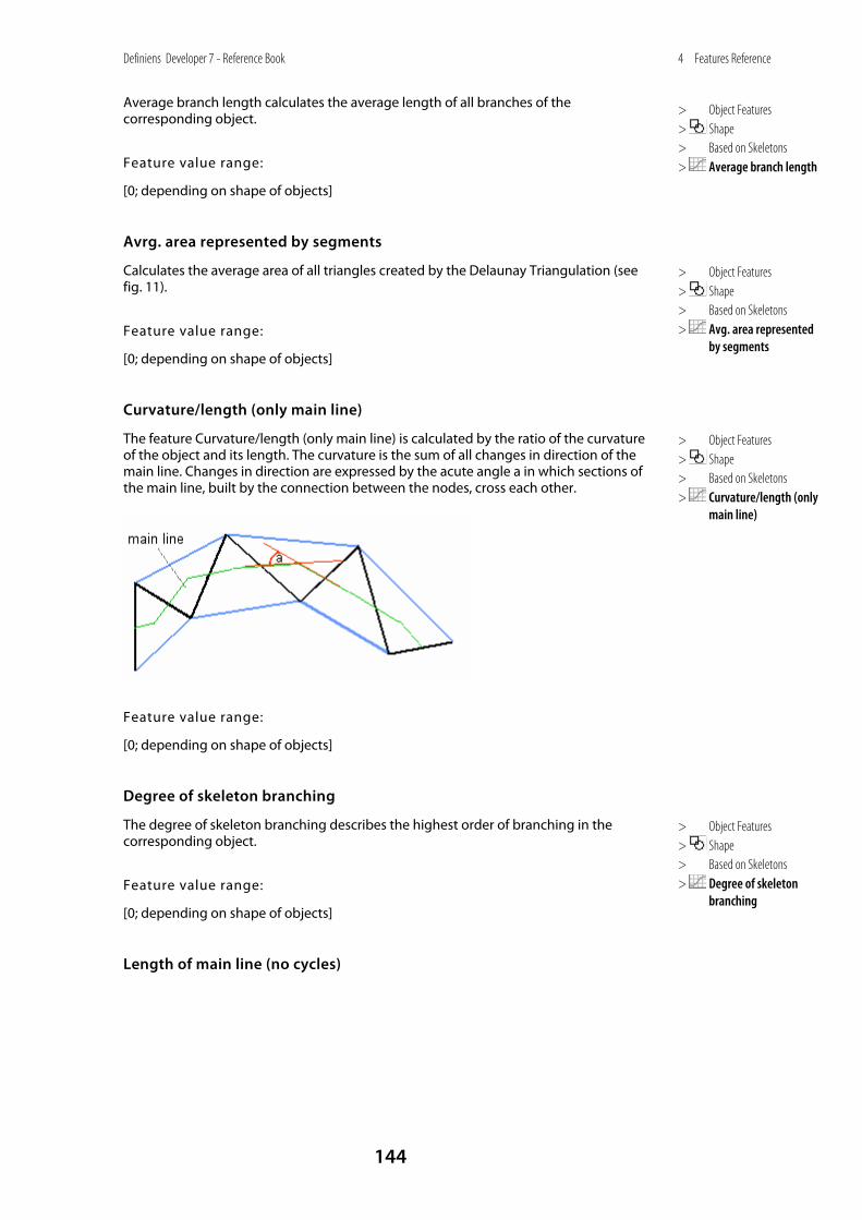
Definiens Developer 7 - Reference Book
144
4 Features Reference
Average branch length calculates the average length of all branches of the corresponding object.
Feature value range:
[0; depending on shape of objects]
Avrg. area represented by segments
Calculates the average area of all triangles created by the Delaunay Triangulation (see fig. 11).
Feature value range:
[0; depending on shape of objects]
Curvature/length (only main line)
The feature Curvature/length (only main line) is calculated by the ratio of the curvature of the object and its length. The curvature is the sum of all changes in direction of the main line. Changes in direction are expressed by the acute angle a in which sections of the main line, built by the connection between the nodes, cross each other.
Feature value range:
[0; depending on shape of objects]
Degree of skeleton branching
The degree of skeleton branching describes the highest order of branching in the corresponding object.
Feature value range:
[0; depending on shape of objects]
Length of main line (no cycles)
> Object Features > Shape > Based on Skeletons > Average branch length
> Object Features > Shape > Based on Skeletons > Avg. area represented
by segments
> Object Features > Shape > Based on Skeletons > Curvature/length (only
main line)
> Object Features > Shape > Based on Skeletons > Degree of skeleton
branching
Definiens Developer 7 - Reference Book
145
4 Features Reference
The length of the main line is calculated by the sum of all distances between its nodes. No cycles means that if an object contains an island polygon, the main line is calculated without regarding the island polygon. In this case the main line could cross the island polygon. Note that this is an internal calculation and could not be visualized like the skeletons regarding the island polygons.
Feature value range:
[0; depending on shape of objects]
Length of main line (regarding cycles)
The length of the main line is calculated by the sum of all distances between its nodes. regarding cycles means that if an object contains an island polygon, the main line is calculated regarding this island polygon. Consequently the main line describes a path around the island polygon. This way also the skeletons for visualization are calculated.
Feature value range:
[0; depending on shape of objects]
Length/Width (only main line)
In the feature Length/width (only main line) the length of an object is divided by its width.
Feature value range:
[0; depending on shape of objects]
Maximum branch length
Maximum branch length calculates the length of the longest branch. The length of a branch is measured from the intersect point of the branch and the main line to the end of the branch.
Feature value range:
[0; depending on shape of objects]
Number of segments
Number of segments is the number of all segments of the main line and the branches.
Feature value range:
[0; depending on shape of objects]
Stddev. curvature (only main line)
The standard deviation of the curvature is the result of the standard deviation of the changes in direction of the main line. Changes in direction are expressed by the acute angle in which sections of the mainline, built by the connection between the nodes, cross each other.
> Object Features > Shape > Based on Skeletons > Length of main line (no
cycles)
> Object Features > Shape > Based on Skeletons > Length of main line
(regarding cycles)
> Object Features > Shape > Based on Skeletons > Length/width (only
main line)
> Object Features > Shape > Based on Skeletons > Maximum branch
length
> Object Features > Shape > Based on Skeletons > Number of segments
> Object Features > Shape > Based on Skeletons > Stddev. curvature (only
main line)
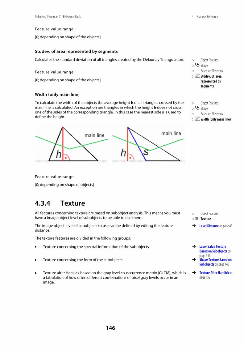
Definiens Developer 7 - Reference Book
146
4 Features Reference
Feature value range:
[0; depending on shape of the objects]
Stddev. of area represented by segments
Calculates the standard deviation of all triangles created by the Delaunay Triangulation.
Feature value range:
[0; depending on shape of the objects]
Width (only main line)
To calculate the width of the objects the average height h of all triangles crossed by the main line is calculated. An exception are triangles in which the height h does not cross one of the sides of the corresponding triangle. In this case the nearest side s is used to define the height.
Feature value range:
[0; depending on shape of objects]
4.3.4 Texture All features concerning texture are based on subobject analysis. This means you must have a image object level of subobjects to be able to use them.
The image object level of subobjects to use can be defined by editing the feature distance.
The texture features are divided in the following groups:
• Texture concerning the spectral information of the subobjects
• Texture concerning the form of the subobjects
• Texture after Haralick based on the gray level co-occurrence matrix (GLCM), which is a tabulation of how often different combinations of pixel gray levels occur in an image.
> Object Features > Shape > Based on Skeletons > Stddev. of area
represented by segments
> Object Features > Shape > Based on Skeletons > Width (only main line)
> Object Features > Texture
Level Distance on page 88
Layer Value Texture Based on Subobjects on page 147
Shape Texture Based on Subobjects on page 148
Texture After Haralick on page 152

Definiens Developer 7 - Reference Book
147
4 Features Reference
4.3.4.1 Layer Value Texture Based on Subobjects These features refer to the spectral information provided by the image layers.
Mean of sub-objects: stddev.
Standard deviation of the different layer mean values of the sub-objects.
At first this feature might appear very similar to the simple standard deviation computed from the single pixel values (layer values), but it might be more meaningful since (a reasonable segmentation assumed) the standard deviation here is computed over homogeneous and meaningful areas. The smaller the sub-objects, the more the feature value approaches the standard deviation calculated from single pixels.
Parameters:
Sv(d) : subobject of an image object v at distance d
⎯ck(u) : mean intensity of layer k of an image object u.
d : level distance
Formula:
Feature value range:
[0; depending on bit depth of data]
Conditions:
If Sv(d) = ∅ ∴ the formula is invalid.
Avrg. mean diff. to neighbors of subobjects
The contrast inside an image object expressed by the average mean difference of all its subobjects for a specific layer.
This feature has a certain spatial reference, as a local contrast inside the area covered by the image object is described. For each single subobject the layer L mean difference (absolute values) to adjacent subobjects of the same superobject is calculated. The feature value is the mean value of the layer L mean differences.
Parameters:
Sv(d) : subobject of an image object v at distance d
⎯Δk(u) : mean difference to neighbor of layer k of an image object u.
d : level distance
> Object Features > Texture > Layer value texture
based on sub-objects
> Object Features > Texture > Layer value texture based
on sub-objects > Mean of sub-objects:
stddev.
> Object Features > Texture > Layer value texture based
on sub-objects > Avrg. mean diff. to
neighbors of subobjects
Definiens Developer 7 - Reference Book
148
4 Features Reference
Formula:
Feature value range:
[0; depending on bit depth of data]
Conditions:
If Sv(d) = ∅ ∴ the formula is invalid
4.3.4.2 Shape Texture Based on Subobjects The following features refer to the form of the sub-objects. The premise to use these features properly is an accurate segmentation of the image, because the sub-objects should be as meaningful as possible.
Area of subobjects: mean
Mean value of the areas of the sub-objects.
Parameters:
Sv(d) : subobject of an image object v at distance d
#Pu : total number of pixels contained in u
d : level distance
Formula:
Feature value range:
[0; scene size]
Condition:
If Sv(d) = ∅ ∴ the formula is invalid.
Area of subobjects: stddev.
Standard deviation of the areas of the sub-objects.
Parameters:
Sv(d) : subobject of an image object v at distance d
> Object Features > Texture > Shape texture based on
sub-objects
> Object Features > Texture > Shape texture based on
sub-objects > Area of sub-objects:
mean
> Object Features > Texture > Shape texture based on
sub-objects > Area of subobjects:
stddev.
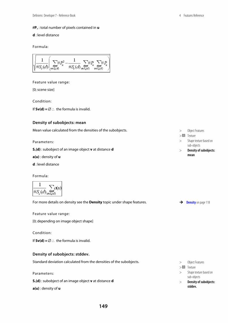
Definiens Developer 7 - Reference Book
149
4 Features Reference
#Pu : total number of pixels contained in u
d : level distance
Formula:
Feature value range:
[0; scene size]
Condition:
If Sv(d) = ∅ ∴ the formula is invalid.
Density of subobjects: mean
Mean value calculated from the densities of the subobjects.
Parameters:
Sv(d) : subobject of an image object v at distance d
a(u) : density of u
d : level distance
Formula:
For more details on density see the Density topic under shape features.
Feature value range:
[0; depending on image object shape]
Condition:
If Sv(d) = ∅ ∴ the formula is invalid.
Density of subobjects: stddev.
Standard deviation calculated from the densities of the subobjects.
Parameters:
Sv(d) : subobject of an image object v at distance d
a(u) : density of u
> Object Features > Texture > Shape texture based on
sub-objects > Density of subobjects:
mean
Density on page 118
> Object Features > Texture > Shape texture based on
sub-objects > Density of subobjects:
stddev.

Definiens Developer 7 - Reference Book
150
4 Features Reference
d : level distance
Formula:
Feature value range:
[0; depending on image object shape]
Condition:
If Sv(d) = ∅ ∴ the formula is invalid.
Asymmetry of subobjects: mean
Mean value of the asymmetries of the subobjects.
Parameters:
Sv(d) : subobject of an image object v at distance d
a(u) : asymmetry of u
d : level distance
Formula:
For more details on asymmetry see the Asymmetry section under shape features.
Feature value range:
[0; depending on image object shape]
Condition:
If Sv(d) = ∅ ∴ the formula is invalid.
Asymmetry of subobjects: stddev.
Standard deviation of the asymmetries of the sub-objects.
Parameters:
Sv(d) : subobject of an image object v at distance d
a(u) : asymmetry of u
d : level distance
> Object Features > Texture > Shape texture based on
sub-objects > Asymmetry of
subobjects: mean
Asymmetry on page 115
> Object Features > Texture > Shape texture based on
sub-objects > Asymmetry of sub-
objects: stddev.
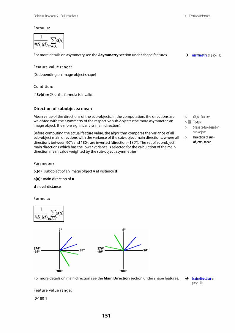
Definiens Developer 7 - Reference Book
151
4 Features Reference
Formula:
For more details on asymmetry see the Asymmetry section under shape features.
Feature value range:
[0; depending on image object shape]
Condition:
If Sv(d) = ∅ ∴ the formula is invalid.
Direction of subobjects: mean
Mean value of the directions of the sub-objects. In the computation, the directions are weighted with the asymmetry of the respective sub-objects (the more asymmetric an image object, the more significant its main direction).
Before computing the actual feature value, the algorithm compares the variance of all sub-object main directions with the variance of the sub-object main directions, where all directions between 90°; and 180°; are inverted (direction - 180°). The set of sub-object main directions which has the lower variance is selected for the calculation of the main direction mean value weighted by the sub-object asymmetries.
Parameters:
Sv(d) : subobject of an image object v at distance d
a(u) : main direction of u
d : level distance
Formula:
For more details on main direction see the Main Direction section under shape features.
Feature value range:
[0-180°]
Asymmetry on page 115
> Object Features > Texture > Shape texture based on
sub-objects > Direction of sub-
objects: mean
Main direction on page 120
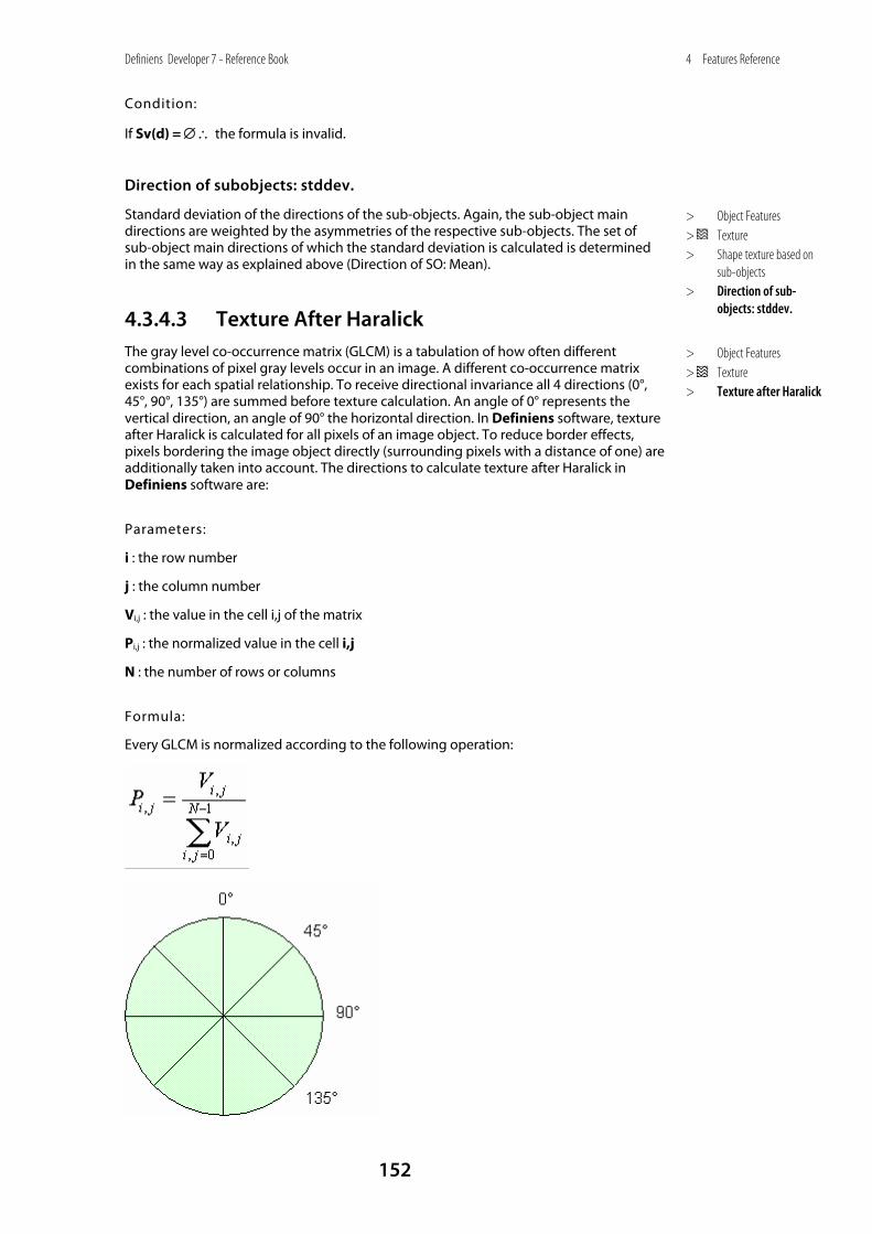
Definiens Developer 7 - Reference Book
152
4 Features Reference
Condition:
If Sv(d) = ∅ ∴ the formula is invalid.
Direction of subobjects: stddev.
Standard deviation of the directions of the sub-objects. Again, the sub-object main directions are weighted by the asymmetries of the respective sub-objects. The set of sub-object main directions of which the standard deviation is calculated is determined in the same way as explained above (Direction of SO: Mean).
4.3.4.3 Texture After Haralick The gray level co-occurrence matrix (GLCM) is a tabulation of how often different combinations of pixel gray levels occur in an image. A different co-occurrence matrix exists for each spatial relationship. To receive directional invariance all 4 directions (0°, 45°, 90°, 135°) are summed before texture calculation. An angle of 0° represents the vertical direction, an angle of 90° the horizontal direction. In Definiens software, texture after Haralick is calculated for all pixels of an image object. To reduce border effects, pixels bordering the image object directly (surrounding pixels with a distance of one) are additionally taken into account. The directions to calculate texture after Haralick in Definiens software are:
Parameters:
i : the row number
j : the column number
Vi,j : the value in the cell i,j of the matrix
Pi,j : the normalized value in the cell i,j
N : the number of rows or columns
Formula:
Every GLCM is normalized according to the following operation:
> Object Features > Texture > Shape texture based on
sub-objects > Direction of sub-
objects: stddev.
> Object Features > Texture > Texture after Haralick
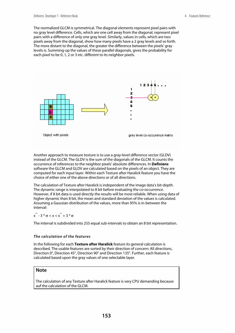
Definiens Developer 7 - Reference Book
153
4 Features Reference
The normalized GLCM is symmetrical. The diagonal elements represent pixel pairs with no gray level difference. Cells, which are one cell away from the diagonal, represent pixel pairs with a difference of only one gray level. Similarly, values in cells, which are two pixels away from the diagonal, show how many pixels have a 2 gray levels and so forth. The more distant to the diagonal, the greater the difference between the pixels' gray levels is. Summing-up the values of these parallel diagonals, gives the probability for each pixel to be 0, 1, 2 or 3 etc. different to its neighbor pixels.
Another approach to measure texture is to use a gray-level difference vector (GLDV) instead of the GLCM. The GLDV is the sum of the diagonals of the GLCM. It counts the occurrence of references to the neighbor pixels' absolute differences. In Definiens software the GLCM and GLDV are calculated based on the pixels of an object. They are computed for each input layer. Within each Texture after Haralick feature you have the choice of either one of the above directions or of all directions.
The calculation of Texture after Haralick is independent of the image data's bit-depth. The dynamic range is interpolated to 8 bit before evaluating the co-occurrence. However, if 8 bit data is used directly the results will be most reliable. When using data of higher dynamic than 8 bit, the mean and standard deviation of the values is calculated. Assuming a Gaussian distribution of the values, more than 95% is in-between the interval:
x⎯ - 3 * σ < x < x⎯ + 3 * σ
The interval is subdivided into 255 equal sub-intervals to obtain an 8 bit representation.
The calculation of the features
In the following for each Texture after Haralick feature its general calculation is described. The usable features are sorted by their direction of concern: All directions, Direction 0°, Direction 45°, Direction 90° and Direction 135°. Further, each feature is calculated based upon the gray values of one selectable layer.
Note
The calculation of any Texture after Haralick feature is very CPU demanding because auf the calculation of the GLCM.
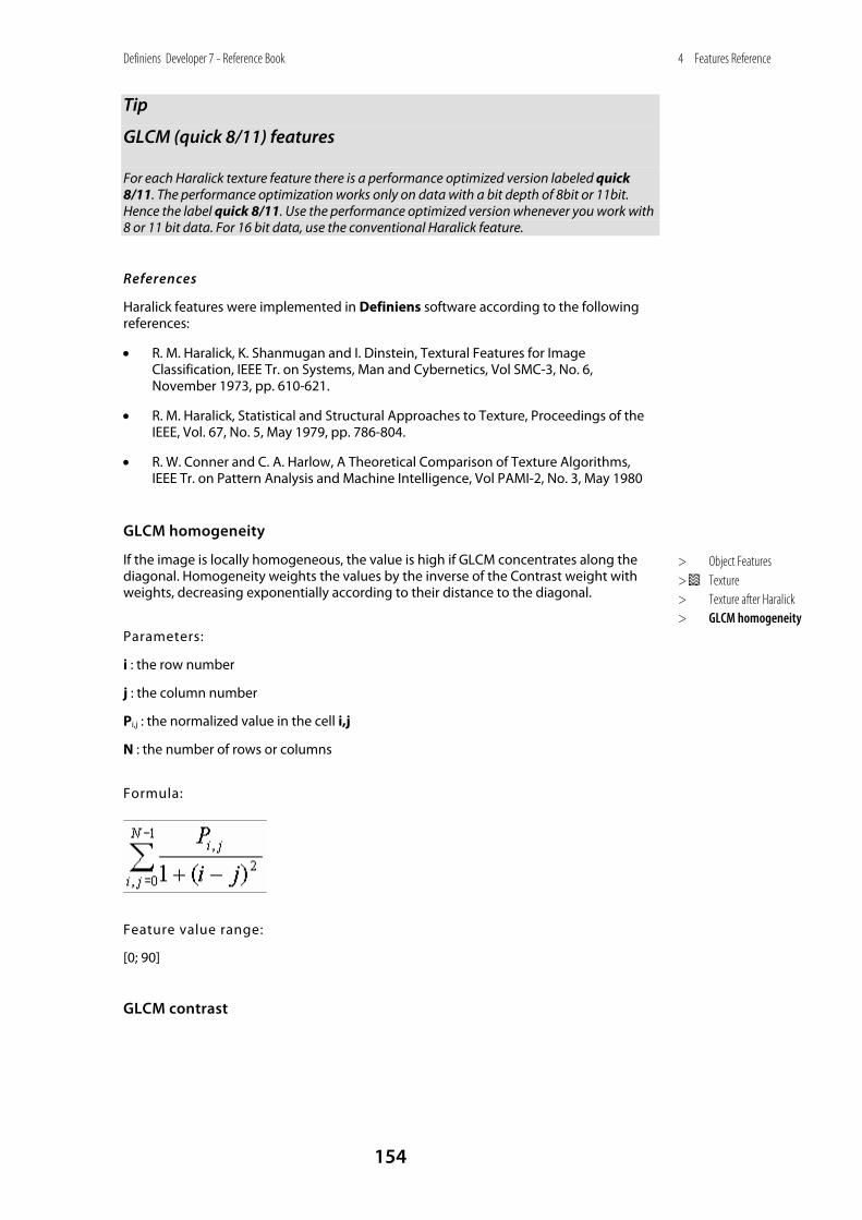
Definiens Developer 7 - Reference Book
154
4 Features Reference
Tip
GLCM (quick 8/11) features
For each Haralick texture feature there is a performance optimized version labeled quick 8/11. The performance optimization works only on data with a bit depth of 8bit or 11bit. Hence the label quick 8/11. Use the performance optimized version whenever you work with 8 or 11 bit data. For 16 bit data, use the conventional Haralick feature.
References
Haralick features were implemented in Definiens software according to the following references:
• R. M. Haralick, K. Shanmugan and I. Dinstein, Textural Features for Image Classification, IEEE Tr. on Systems, Man and Cybernetics, Vol SMC-3, No. 6, November 1973, pp. 610-621.
• R. M. Haralick, Statistical and Structural Approaches to Texture, Proceedings of the IEEE, Vol. 67, No. 5, May 1979, pp. 786-804.
• R. W. Conner and C. A. Harlow, A Theoretical Comparison of Texture Algorithms, IEEE Tr. on Pattern Analysis and Machine Intelligence, Vol PAMI-2, No. 3, May 1980
GLCM homogeneity
If the image is locally homogeneous, the value is high if GLCM concentrates along the diagonal. Homogeneity weights the values by the inverse of the Contrast weight with weights, decreasing exponentially according to their distance to the diagonal.
Parameters:
i : the row number
j : the column number
Pi,j : the normalized value in the cell i,j
N : the number of rows or columns
Formula:
Feature value range:
[0; 90]
GLCM contrast
> Object Features > Texture > Texture after Haralick > GLCM homogeneity
Definiens Developer 7 - Reference Book
155
4 Features Reference
Contrast is the opposite of homogeneity. It is a measure of the amount of local variation in the image. It increases exponentially as (i-j) increases.
Parameters:
i : the row number
j : the column number
Pi,j : the normalized value in the cell i,j
N : the number of rows or columns
Formula:
Feature value range:
[0; 90]
GLCM dissimilarity
Similar to contrast, but increases linearly. High if the local region has a high contrast.
Parameters:
i : the row number
j : the column number
Pi,j : the normalized value in the cell i,j
N : the number of rows or columns
Formula:
Feature value range:
[0; 90]
GLCM entropy
> Object Features > Texture > Texture after Haralick > GLCM Contrast
> Object Features > Texture > Texture after Haralick > GLCM dissimilarity
Definiens Developer 7 - Reference Book
156
4 Features Reference
The value for entropy is high, if the elements of GLCM are distributed equally. It is low if the elements are close to either 0 or 1. Since ln(0) is undefined, it is assumed that 0 * ln(0) = 0.
Parameters:
i : the row number
j : the column number
Pi,j : the normalized value in the cell i,j
N : the number of rows or columns
Formula:
Feature value range:
[0; 90]
GLCM ang. 2nd moment
Parameters:
i : the row number
j : the column number
Pi,j : the normalized value in the cell i,j
N : the number of rows or columns
Formula:
Feature value range:
[0; 90]
GLCM mean
The GLCM mean is the average expressed in terms of the GLCM. The pixel value is not weighted by its frequency of occurrence itself, but by the frequency of its occurrence in combination with a certain neighbor pixel value.
Parameters:
i : the row number
> Object Features > Texture > Texture after Haralick > GLCM entropy
> Object Features > Texture > Texture after Haralick > GLCM ang. 2nd
moment
> Object Features > Texture > Texture after Haralick > GLCM Mean
Definiens Developer 7 - Reference Book
157
4 Features Reference
j : the column number
Pi,j : the normalized value in the cell i,j
N : the number of rows or columns
Formula:
Feature value range:
[0; 90]
GLCM stddev
GLCM standard deviation uses the GLCM, therefore it deals specifically with the combinations of reference and neighbor pixels. Thus, it is not the same as the simple standard deviation of gray levels in the original image.
Calculating the standard deviation using i or j gives the same result, since the GLCM is symmetrical.
Standard deviation is a measure of the dispersion of values around the mean. It is similar to contrast or dissimilarity.
Parameters:
i : the row number
j : the column number
Pi,j : the normalized value in the cell i,j
N : the number of rows or columns
μi,j : GLCM mean
Formula:
Standard Deviation:
Feature value range:
[0; 90]
> Object Features > Texture > Texture after Haralick > GLCM StdDev.
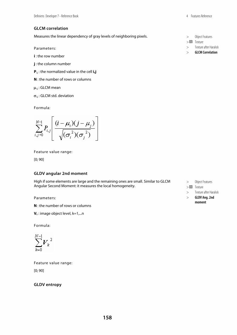
Definiens Developer 7 - Reference Book
158
4 Features Reference
GLCM correlation
Measures the linear dependency of gray levels of neighboring pixels.
Parameters:
i : the row number
j : the column number
Pi,j : the normalized value in the cell i,j
N : the number of rows or columns
μi,j : GLCM mean
σi,j : GLCM std. deviation
Formula:
Feature value range:
[0; 90]
GLDV angular 2nd moment
High if some elements are large and the remaining ones are small. Similar to GLCM Angular Second Moment: it measures the local homogeneity.
Parameters:
N : the number of rows or columns
Vk : image object level, k=1,...n
Formula:
Feature value range:
[0; 90]
GLDV entropy
> Object Features > Texture > Texture after Haralick > GLCM Correlation
> Object Features > Texture > Texture after Haralick > GLDV Ang. 2nd
moment
Definiens Developer 7 - Reference Book
159
4 Features Reference
The values are high if all elements have similar values. It is the opposite of GLDV Angular Second Moment.
Parameters:
i : the row number
j : the column number
Pi,j : the normalized value in the cell i,j
N : the number of rows or columns
Vk : image object level, k=1,...n
Formula:
Since ln(0) is undefined, it is assumed that 0 * ln(0) = 0:
Feature value range:
[0; 90]
GLDV mean
The mean is mathematically equivalent to the GLCM Dissimilarity measure above. It is only left here for compatibility reasons.
Parameters:
N : the number of rows or columns
Vk : image object level, k=1,...n
Formula:
Feature value range:
[0; 90]
GLDV contrast
> Object Features > Texture > Texture after Haralick > GLDV Entropy
> Object Features > Texture > Texture after Haralick > GLDV Mean
Definiens Developer 7 - Reference Book
160
4 Features Reference
It is mathematically equivalent to the GLCM Contrast measure above. It is only left here for compatibility reasons.
Parameters:
N : the number of rows or columns
Vk : image object level, k=1,...n
k :
Formula:
Feature value range:
[0; 90]
GLCM and GLDV (quick 8/11)
For each Haralick texture feature there is a performance optimized version labeled quick 8/11.
The performance optimization works only on data with a bit depth of 8bit or 11bit. Hence the label quick 8/11. Use the performance optimized version whenever you work with 8 or 11 bit data. For 16 bit data, use the conventional Haralick feature.
4.3.5 Variables All object variables are listed here.
[name of a local variable]
Define variables to describe interim values. Variables are used as:
• constants
• fixed and dynamic thresholds
• store temporary and final results
Variables should be used to store "tools" with which you may fine-tune your rule-sets for similar projects.
For detailed description on how to create a variable refer to the Create a Variable section.
Feature value range:
[-∞; ∞]
> Object Features > Texture > Texture after Haralick > GLDV Contrast
> Object Features > Variables
> Object Features > Variables > [name of a local
variable]
Definiens Developer 7 - Reference Book
161
4 Features Reference
4.3.6 Hierarchy Hierarchy features refer to the embedding of an image object in the entire image object hierarchy.
Level
The number of the image object level an image object is situated in. You will need this feature if you perform classification on different image object levels to define which class description is valid for which image object level.
Parameters:
Uv(d) : superobjects of an image object v at distance d
Formula:
Feature value range:
[1; number of image object levels]
Conditions:
To use this feature you need to have more than one image object levels.
Number of higher levels
The number of image object levels situated above the image object level the object of concern is situated in. This is identical to the number of superobjects an image object may have.
Parameters:
d : distance between neighbors
Sv(d) : subobjects of an image object v at a distance d
Formula:
Feature value range:
[1; number of image object levels -1]
Number of neighbors
The number of the direct neighbors of an image object (i.e., neighbors with which it has a common border) on the same image object level in the image object hierarchy.
> Object Features > Hierarchy
> Object Features > Hierarchy > Level
> Object Features > Hierarchy > Number of higher
levels
> Object Features > Hierarchy > Number of neighbors
Definiens Developer 7 - Reference Book
162
4 Features Reference
Parameters:
Nv(d) : neighbors of an image object v at a distance d
Formula:
#Nv(d)
Feature value range:
[0; number of pixels of entire scene]
Number of subobjects
Concerning an image object, the number of subobjects that are located on the next lower image object level in the image object hierarchy.
Parameters:
Sv(d) : subobjects of an image object v at a distance d
Formula:
#Sv(d)
Feature value range:
[0; number of pixels of entire scene]
Number of sublevels
The number of image object levels situated below the image object level the object of concern is situated in.
Parameters:
d : distance between neighbors
Uv(d) : superobjects of an image object v at a distance d
Formula:
Feature value range:
[1; number of image object levels -1]
> Object Features > Hierarchy > Number of sub-objects
> Object Features > Hierarchy > Number of sublevels
Definiens Developer 7 - Reference Book
163
4 Features Reference
4.3.7 Thematic Attributes Thematic attributes are used to describe an image object using information provided by thematic layers.
If your project contains a thematic layer, the object's thematic properties (taken from the thematic layer) can be evaluated. Depending on the attributes of the thematic layer, a large range of different features becomes available.
Note
If the currently open project does include a thematic layer, Thematic attributes features are not listed in the feature tree.
[name of the thematic objects attribute]
If existing, Thematic Objects Attribute features referring to a thematic layer are listed in the feature tree. Available only for image objects that overlap with one or no thematic object.
Thematic object ID
The identification number (ID) of a thematic object. Available only for image objects that overlap with one or no thematic object.
Number of overlapping thematic objects
The number of overlapping thematic objects. Available only for image object overlaps with one or no thematic object. Available only for image objects that overlap with several thematic objects.
Feature value range:
[0; number of thematic objects]
4.4 Class-Related Features
4.4.1 Customized
[name of a customized feature]
If existing, customized features referring to other classes are displayed here.
> Object Features > Thematic attributes
> Object Features > Thematic Attributes > [name of the thematic
objects attribute]
> Object Features > Thematic Attributes > Thematic object ID
> Object Features > Thematic Attributes > Number of overlapping
thematic objects
> Class-Related Features
> Class-Related Features > Customized
> Class-Related Features > Customized > [name of a customized
feature]
Definiens Developer 7 - Reference Book
164
4 Features Reference
4.4.2 Relations to Neighbor Objects Use the following features to describe an image object by the classification of other image objects on the same image object level in the image object hierarchy.
Existence of
Existence of an image object assigned to a defined class in a certain perimeter (in pixels) around the image object concerned. If an image object of the defined classification is found within the perimeter, the feature value is 1 (= true), otherwise it would be 0 (= false). The radius defining the perimeter can be determined by editing the feature distance.
Formula:
0 if Nv(d,m) = ∅
1 if Nv(d,m) ≠ ∅
Feature value range:
[0,1]
Number of
Number of objects belonging to the selected class in a certain distance (in pixels) around the image object.
Parameters:
v : image object
d : distance between neighbors
m : a class containing image objects
Expression:
#Nv(d,m)
Feature value range:
[0, ∞]
Border to
The absolute border of an image object shared with neighboring objects of a defined classification. If you use georeferenced data, the feature value is the real border to image objects of a defined class; otherwise it is the number of pixel edges shared with the adjacent image objects, as by default the pixel edge-length is 1.
Parameters:
b(v,u) : topological relation border length
Nv(d) : neighbors to an image object v at a distance d
> Class-Related Features > Relations to neighbor
objects
> Class-Related Features > Relations to neighbor
objects > Existence of
> Class-Related Features > Relations to neighbor
objects > Number of
> Class-Related Features > Relations to neighbor
objects > Border to
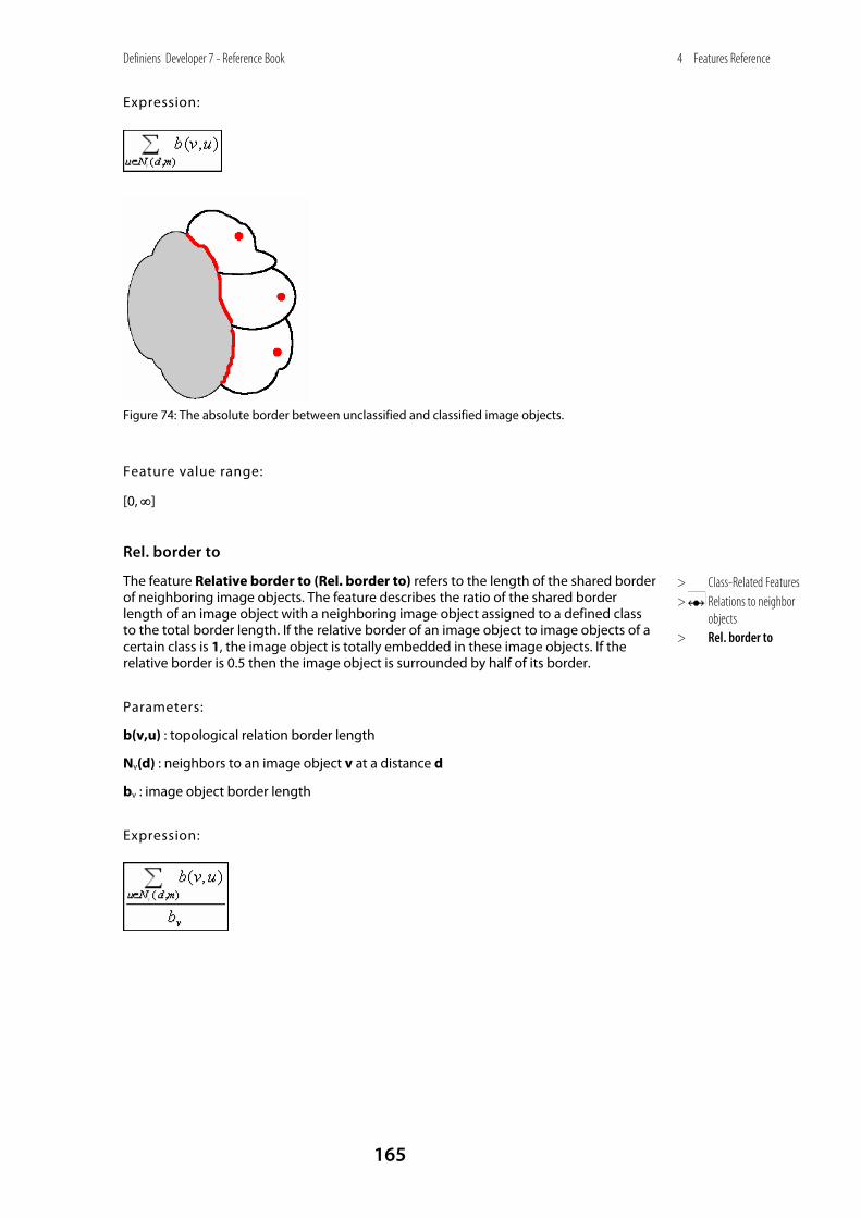
Definiens Developer 7 - Reference Book
165
4 Features Reference
Expression:
Figure 74: The absolute border between unclassified and classified image objects.
Feature value range:
[0, ∞]
Rel. border to
The feature Relative border to (Rel. border to) refers to the length of the shared border of neighboring image objects. The feature describes the ratio of the shared border length of an image object with a neighboring image object assigned to a defined class to the total border length. If the relative border of an image object to image objects of a certain class is 1, the image object is totally embedded in these image objects. If the relative border is 0.5 then the image object is surrounded by half of its border.
Parameters:
b(v,u) : topological relation border length
Nv(d) : neighbors to an image object v at a distance d
bv : image object border length
Expression:
> Class-Related Features > Relations to neighbor
objects > Rel. border to
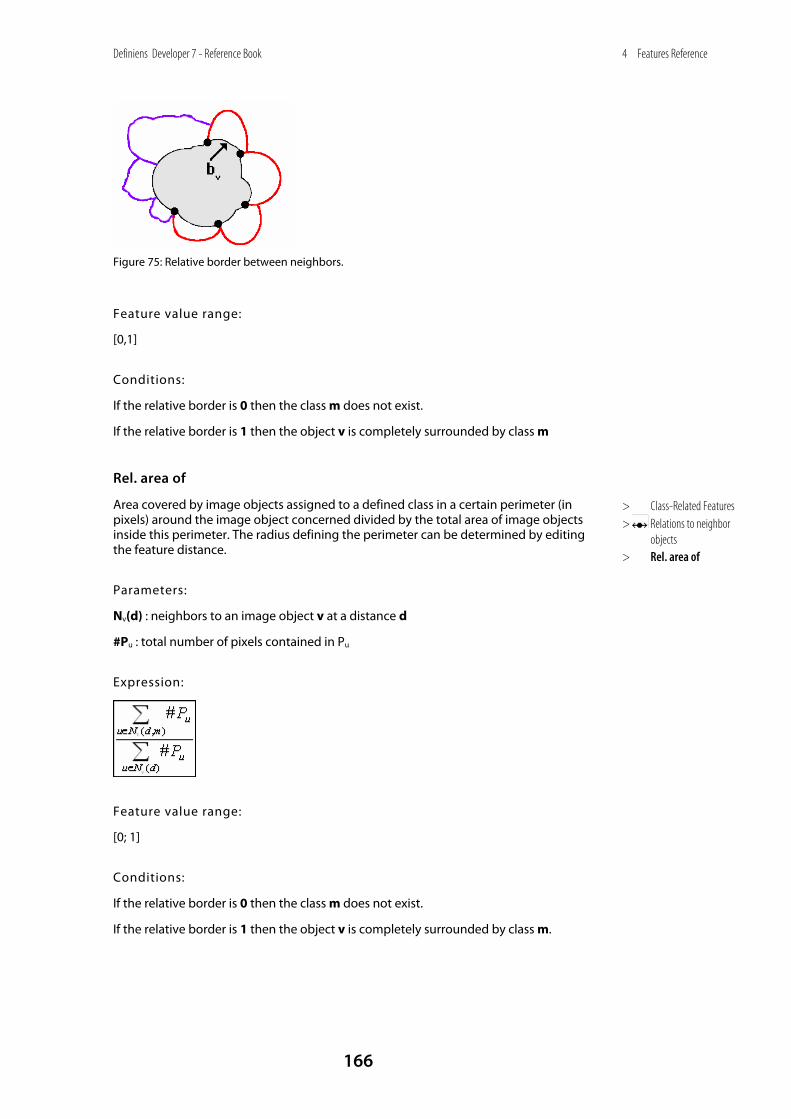
Definiens Developer 7 - Reference Book
166
4 Features Reference
Figure 75: Relative border between neighbors.
Feature value range:
[0,1]
Conditions:
If the relative border is 0 then the class m does not exist.
If the relative border is 1 then the object v is completely surrounded by class m
Rel. area of
Area covered by image objects assigned to a defined class in a certain perimeter (in pixels) around the image object concerned divided by the total area of image objects inside this perimeter. The radius defining the perimeter can be determined by editing the feature distance.
Parameters:
Nv(d) : neighbors to an image object v at a distance d
#Pu : total number of pixels contained in Pu
Expression:
Feature value range:
[0; 1]
Conditions:
If the relative border is 0 then the class m does not exist.
If the relative border is 1 then the object v is completely surrounded by class m.
> Class-Related Features > Relations to neighbor
objects > Rel. area of
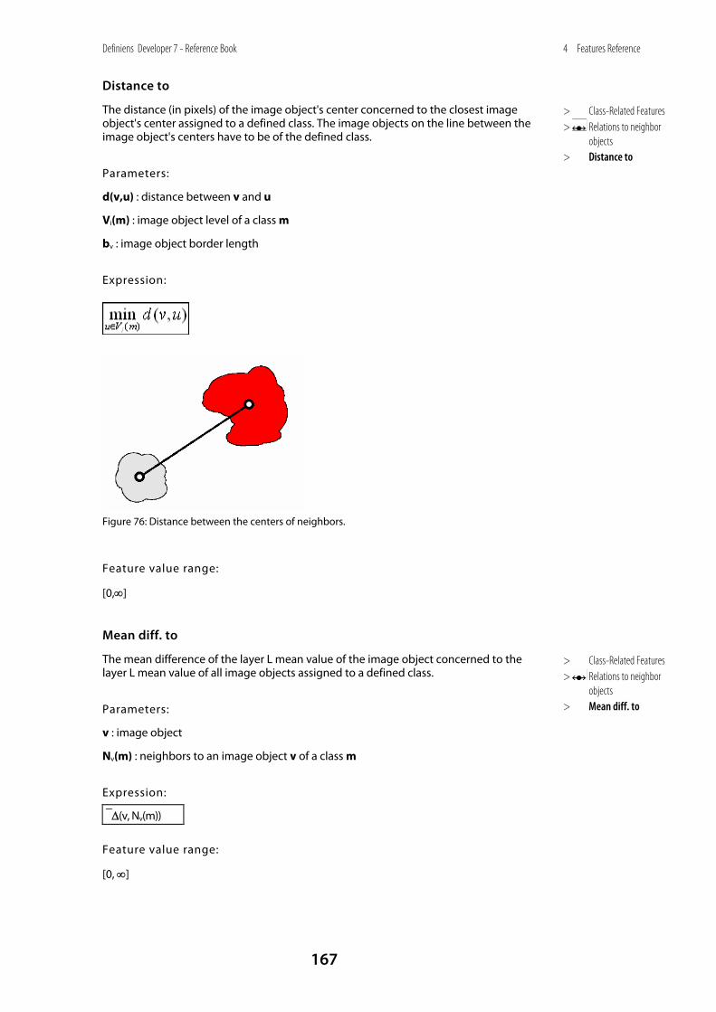
Definiens Developer 7 - Reference Book
167
4 Features Reference
Distance to
The distance (in pixels) of the image object's center concerned to the closest image object's center assigned to a defined class. The image objects on the line between the image object's centers have to be of the defined class.
Parameters:
d(v,u) : distance between v and u
Vi(m) : image object level of a class m
bv : image object border length
Expression:
Figure 76: Distance between the centers of neighbors.
Feature value range:
[0,∞]
Mean diff. to
The mean difference of the layer L mean value of the image object concerned to the layer L mean value of all image objects assigned to a defined class.
Parameters:
v : image object
Nv(m) : neighbors to an image object v of a class m
Expression:
⎯Δ(v, Nv(m))
Feature value range:
[0, ∞]
> Class-Related Features > Relations to neighbor
objects > Distance to
> Class-Related Features > Relations to neighbor
objects > Mean diff. to
Definiens Developer 7 - Reference Book
168
4 Features Reference
4.4.3 Relations to Subobjects These features refer to existing class assignments of image objects on a lower image object level in the image object hierarchy. Which of the lower image object levels to refer to can be determined by editing the feature distance.
Existence of
Checks if there is at least one subobject assigned to a defined class. If there is one, the feature value is 1 (= true), otherwise the feature value is 0 (= false).
Parameters:
v : image object
d : distance between neighbors
m : a class containing image objects
Formula:
0 if Sv(d,m) = ∅
1 if Sv(d,m) ≠ ∅
Feature value range:
[0,1]
Number of
The number of subobjects assigned to a defined class.
Parameters:
v : image object
d : distance between neighbors
m : a class containing image objects
Expression:
#Sv(d,m)
Feature value range:
[0, ∞]
Area of
The absolute area covered by subobjects assigned to a defined class. If your data are georeferenced, the feature value represents the real area.
Parameters:
d: distance
> Class-Related features > Relations to sub objects
> Class-Related features > Relations to sub objects > Existence of
> Class-Related features > Relations to sub objects > Number of
> Class-Related features > Relations to sub objects > Area of

Definiens Developer 7 - Reference Book
169
4 Features Reference
m: class
M: subobjects in class M
Expression:
Feature Value Range:
[0;∞]
Rel. area of
The area covered by subobjects assigned to a defined class divided by the total area of the image object concerned.
Parameters:
d: distance
m: class
M: subobjects in class M
Expression:
Feature Value Range:
[0;1]
Clark aggregation index
For a superobject the Clark aggregation index gives evidence about the spatial distribution of its subobjects of a certain class.
Parameters:
D(x) : mean spacial Distance to next neighbor of the subobjects of the class x
N(x) : Number of subobjects of class x
A: Number of pixels of the superobject (Area)
> Class-Related features > Relations to sub objects > Rel. area of
> Class-Related features > Relations to sub objects > Clark aggregation
index
Definiens Developer 7 - Reference Book
170
4 Features Reference
Obs_mean_dist : Observed mean distance of sub objects to their spatial nearest neighbor
Exp_mean_dist : Expected mean distance of sub objects to their spatial nearest neighbor
CAI : Clark aggregation index
Formula:
Feature Value Range:
[0, 2.149]
0 : heavily clumped subobjects
1 : homogeneous spatial distribution of subobjects
2.149 : hexagonal distribution (edges of a honeycomb) of the subobjects
4.4.4 Relations to Superobjects This feature refers to existing class assignments of image objects on a higher image object level in the image object hierarchy.
Existence of
Checks if the superobject is assigned to a defined class. If this is true, the feature value is 1, otherwise 0.
Parameters:
v : image object
d : distance between neighbors
m : a class containing image objects
Formula:
0 if Uv(d,m) = ∅
1 if Uv(d,m) ≠ ∅
Feature Value Range:
[0,1]
> Class-Related features > Relations to super
objects
> Class-Related features > Relations to super objects > Existence of
Definiens Developer 7 - Reference Book
171
4 Features Reference
4.4.5 Relations to Classification
Membership to
In some cases it is important to incorporate the membership value to different classes in one class. This function allows explicit addressing of the membership values to different classes. If the membership value is below the assignment threshold, this value turns to 0.
Parameters:
v : image object
m : a class containing image objects
: stored membership value of an image object v to a class m
Expression:
Feature value range:
[0,1]
Classified as
The idea of this feature is to enable the user to refer to the classification of an image object without regard to the membership value. It can be used to freeze a classification.
Parameters:
v : image object
m : a class containing image objects
Expression:
m(v)
Feature value range:
[0,1]
Classification value of
> Class-Related features > Relations to
Classification
> Class-Related Features > Relations to Classification > Membership to
> Class-Related Features > Relations to Classification > Classified as

Definiens Developer 7 - Reference Book
172
4 Features Reference
This feature Classification value of allows you to explicitly address the membership values to all classes. As opposed to the feature Membership to it is possible to apply all membership values to all classes without restrictions.
Parameters:
v : image object
m : a class containing image objects
ϕ(v,m) : fuzzy membership value of an image object v to a class m
Expression:
ϕ(v,m)
Feature value range:
[0,1]
4.4.5.1 Class Name The Class name feature returns the name of the class (or superclass) of an image object (or its superobject).
Parameters:
Distance in class hierarchy specifies the number of hierarchical levels when navigating from class to superclass. Using a distance of '0' the class name is returned, a distance of '1' will return the superclass name and so on.
Distance in image object hierarchy specifies the number of hierarchical levels when navigating from object to superobject. Using a distance of '0' the class of the image object is used as a starting point for the navigation in the class hierarchy, a distance of '1' will start at the class of the superobject.
4.4.5.2 Class Color The Class color feature returns either the Red, Green or Blue color component of the class (or superclass) of an image object (or its superobject).
Parameters:
Color component is Red, Green or Blue.
Distance in class hierarchy specifies the number of hierarchical levels when navigating from class to superclass. Using a distance of '0' the class name is returned, a distance of '1' will return the superclass name and so on.
Distance in image object hierarchy specifies the number of hierarchical levels when navigating from object to superobject. Using a distance of '0' the class of the image object is used as a starting point for the navigation in the class hierarchy, a distance of '1' will start at the class of the superobject.
> Class-Related Features > Relations to Classification > Classification value of
> Class-Related Features > Relations to Classification > Class Name
> Class-Related Features > Relations to Classification > Class Color
Definiens Developer 7 - Reference Book
173
4 Features Reference
4.5 Scene Features
4.5.1 Variables All scene variables are listed here.
[name of a scene variable]
Define variables to describe interim values.
4.5.2 Class-Related
Number of classified objects
The absolute number of all image objects of the selected class on all image object levels.
Parameters:
V(m) : all image objects of a class m
m : a class containing image objects
Expression:
#V(m)
Feature value range:
[0,number of image objects]
Number of samples per class
The number of all samples of the selected class on all image object levels.
Parameters:
m : a class
Feature value range:
[0,number of samples]
Area of classified objects
> Scene Features
> Scene Features > Variables
> Scene features > Variables > [name of a global
variable]
> Scene features > Class-Related
> Scene features > Class-Related > Number of classified
objects
> Scene features > Class-Related > Number of samples per
class
Definiens Developer 7 - Reference Book
174
4 Features Reference
The absolute area of all image objects of the selected class on all image object levels in pixel.
Parameters:
v : image object
m : a class containing image objects
V(m) : all image objects of a class m
#Pv : total number of pixels contained in Pv
Expression:
Feature Value Range:
[0,sx*sy]
Layer mean of classified objects
The mean of all image objects of the selected class on the selected image object levels.
Parameters:
v : image object
m : a class containing image objects
V(m) : all image objects of a class m
⎯ck(v) : mean intensity layer of an image object v
Expression:
Feature value range:
[0,1]
Layer stddev. of classified objects
The standard deviation of all image objects of the selected class on the selected image object levels.
Parameters:
v : image object
m : a class containing image objects
> Scene features > Class-Related > Area of classified
objects Area on page 115
> Scene features > Class-Related > Layer mean of
classified objects
> Scene features > Class-Related > Layer stddev. of
classified objects
Definiens Developer 7 - Reference Book
175
4 Features Reference
V(m) : all image objects of a class m
ck(v) : image layer value of an image object v
Formula:
Feature value range:
[0,1]
4.5.2.1 Class Variables All class variables are listed here.
[name of a class variable]
A variable that use classes as values. In a rule set they can be used instead of an ordinary classes where needed.
4.5.3 Scene-Related
Existence of object level
Existence of a defined image object level. If the image object level with the given name exists within the project the feature value is 1 (= true), otherwise it is 0 (= false).
Parameter:
• Image object level name
Feature value range:
[0,1]
Existence of image layer
Existence of a defined image layer. If the image layer with the given alias exists within the project the feature value is 1 (= true), otherwise it is 0 (= false).
Parameter:
• Image layer alias
Feature value range:
[0,1]
> Scene features > Class-Related > Class Variable
> Scene features > Class-Related > Class Variable > [name of a class
variable]
> Scene features > Scene-Related
> Scene features > Scene-Related > Existence of object
level
> Scene features > Scene-Related > Existence of image
layer
Definiens Developer 7 - Reference Book
176
4 Features Reference
Existence of thematic layer
Existence of a defined thematic layer. If the thematic layer with the given alias exists within the project the feature value is 1 (= true), otherwise it is 0 (= false).
Parameter:
• Thematic layer alias
Feature value range:
[0,1]
Mean of scene
Mean value for the selected layer.
Expression:
⎯ck
Stddev.
Standard deviation for the selected layer.
Expression:
σk
Smallest actual pixel value
Darkest actual intensity value of all pixel values of the selected layer.
Expression:
c'kmin
Feature value range:
[ckmin, ck
max]
Smallest actual pixel value
Brightest actual intensity value of the selected layer.
Expression:
c'kmax
Feature value range:
[ckmin, ck
max]
> Scene features > Scene-Related > Existence of thematic
layer
> Scene features > Scene-Related > Mean of Scene
> Scene features > Scene-Related > StdDev
> Scene features > Scene-Related > Smallest actual pixel
value
> Scene features > Scene-Related > Largest actual pixel
value
Definiens Developer 7 - Reference Book
177
4 Features Reference
Image size X
Vertical size x of the image in the display unit.
Expression:
sx
Image size Y
Horizontal size y of the image in the display unit.
Expression:
sy
Number of image layers
Number of layers K which are imported in the scene.
Number of objects
Number of image objects of any class on all image object levels of the scene including unclassified image objects.
Expression:
#V
Feature value range:
[0,1]
Number of pixels
Number of pixels in the pixel layer of the image.
Parameters:
sx : image size x
sy : image size y
(sx,sy) : scene size
Expression:
sx*sy
Feature value range:
[0,1]
> Scene features > Scene-Related > Image size X
> Scene features > Scene-Related > Image size X
> Scene features > Scene-Related > Number of objects
> Scene features > Scene-Related > Number of objects
> Scene features > Scene-Related > Number of pixels
Definiens Developer 7 - Reference Book
178
4 Features Reference
Number of Samples
Number of all samples on all image object levels of the scene.
Feature value range:
[0,number of samples]
Number of thematic layers
Number of layers T which are imported in the scene.
4.5.3.1 User name This feature returns the user name.
Pixel Resolution
The resolution of the scene as given in the metadata of the project. The resulting number represents the size of a pixel in coordinate system unit.
The value is 1 if no resolution is set.
4.6 Process-Related Features
4.6.1 Customized
diff. PPO
Parameters:
v : image object
f : any feature
ρ :
Formula:
f(v) - f(ρ)
> Scene features > Scene-Related > Number of samples
> Scene features > Scene-Related > Number of thematic
layers
> Scene features > Scene-Related > User name
> Scene features > Scene-Related > Pixel resolution
> Process-Related features
> Process-Related features > Customized
> Process-Related features > Customized > diff. PPO
Definiens Developer 7 - Reference Book
179
4 Features Reference
Feature value range:
The range depends on the value of the feature in use.
Conditions:
If f(ρ) =0 ∴ the formula is undefined
ratio PPO
Parameters:
v : image object
f : any feature
ρ :
Formula:
Feature value range:
The range depends on the value of the feature in use.
Conditions:
If f(ρ) =0 ∴ the formula is undefined
[name of a customized feature]
If existing, customized features referring to a Parent Process Object (PPO) are listed in the feature tree.
Border to PPO
Parameters:
b(v,ρ) : topological relation border length with the PPO
Formula:
b(v,ρ)
> Process-Related features > Customized > ratio PPO
> Process-Related features > Border to PPO
Definiens Developer 7 - Reference Book
180
4 Features Reference
Feature value range:
[0,max size]
Elliptic Dist. from PPO
Measures elliptic distance of an object to its Parent Process Object (PPO).
Parameters:
⎯xv :
⎯yv :
Formula:
Feature value range:
[0,∞]
Rel. border to PPO
The ratio of the border length of an image object shared with the Parent Process Object (PPO) to its total border length.
Parameters:
bv : image object border length
b(v,ρ) : topological relation border length with the PPO
Formula:
Feature value range:
[0,1]
Same superobject as PPO
Checks whether this image object and its Parent Process Object (PPO) are parts of the same superobject.
Parameters:
v : image object
ρ :
Uv(d) : superobject of an image object v at a distance d
> Process-Related features > Elliptic Dist. from PPO
> Process-Related features > Rel. border to PPO
> Process-Related features > Same super object as
PPO

Definiens Developer 7 - Reference Book
181
4 Features Reference
Formula:
Feature value range:
[0,1]
4.7 Customized
4.7.1 Largest possible pixel value This feature returns the largest possible pixel value for a chosen layer. For example, the value displayed for a 8 bit image would be 255 and the value for a 16 bit image would be 65536.
Parameter
Layer: Use the drop-down list to select an image layer.
4.7.2 Smallest possible pixel value This feature returns smallest possible pixel value for a layer. This value will often be 0, but can be a negative value for some types of image data.
Parameter
Layer: Use the drop-down list to select a layer for which you want to display the lowest possible value.
[name of a metadata item]
A metadata item that can be used as a feature in rule set development.
To make external metadata available to the feature tree, you have to convert it within data import procedures to get an internal metadata definitio
4.8 Metadata All metadata items are listed here.
> Customized
> Customized> Create new "Largest
possible pixel value"
> Customized> Create new "Smallest
possible pixel value"
> Metadata > [name of a metadata
item] About Metadata as a
Source of Information on page 188
User Guide sections: Create Project and Customized Import
> Metadata
Definiens Developer 7 - Reference Book
182
4 Features Reference
4.9 Feature Variables All feature variables are listed here.
[name of a feature variable]
A variable that use features as values.
In a rule set they can be used like that feature. It returns the same value as the feature to which it points. It uses the unit of whatever feature is assigned as a variable. It is possible to create a feature variable without a feature assigned, but the calculation value would be invalid.
4.10 Use Customized Features Customized features allow you to create new features that are adapted to your needs. Customized features are composed of arithmetic and relational features. All customized features are based on the features shipped with Definiens Developer as well as newly created customized features.
• Arithmetic features, are composed of existing features, variables (Definiens Developer only), and constants, which are combined via arithmetic operations. Arithmetic features can be composed of multiple features but apply only to a single object.
• Relational features, are used to compare a particular feature of one object to those of related objects of a specific class within a specified distance. Related objects are surrounding objects (neighbors), sub-objects, superobjects, sub-objects of a superobject or a complete image object level. Relational features are composed of only a single feature but refer to a group of related objects.
4.10.1 Create Customized Features The Manage Customized Features dialog box allows you to add, edit, copy, and delete customized features. It enables you to create new arithmetic as well as relational features based on the existing ones.
1. To open the Manage Customized Features dialog box, do one of the following:
• On the menu bar click on Tools and then select Manage Customized Features.
• On the Tools toolbar click on the Manage Customized Features icon.
> Feature Variables
> Feature variables > [name of a feature
variable]
Manage Customized Features
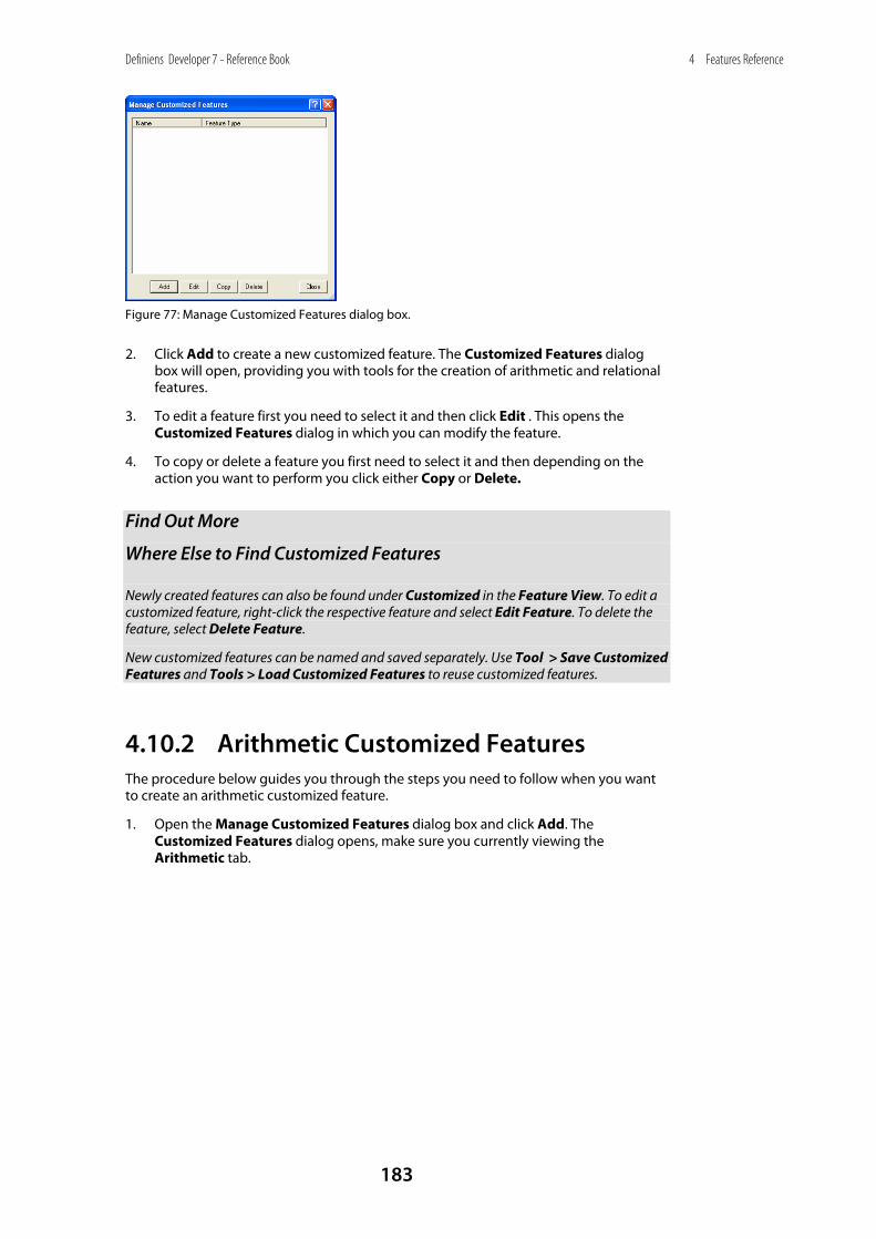
Definiens Developer 7 - Reference Book
183
4 Features Reference
Figure 77: Manage Customized Features dialog box.
2. Click Add to create a new customized feature. The Customized Features dialog box will open, providing you with tools for the creation of arithmetic and relational features.
3. To edit a feature first you need to select it and then click Edit . This opens the Customized Features dialog in which you can modify the feature.
4. To copy or delete a feature you first need to select it and then depending on the action you want to perform you click either Copy or Delete.
Find Out More
Where Else to Find Customized Features
Newly created features can also be found under Customized in the Feature View. To edit a customized feature, right-click the respective feature and select Edit Feature. To delete the feature, select Delete Feature.
New customized features can be named and saved separately. Use Tool > Save Customized Features and Tools > Load Customized Features to reuse customized features.
4.10.2 Arithmetic Customized Features The procedure below guides you through the steps you need to follow when you want to create an arithmetic customized feature.
1. Open the Manage Customized Features dialog box and click Add. The Customized Features dialog opens, make sure you currently viewing the Arithmetic tab.
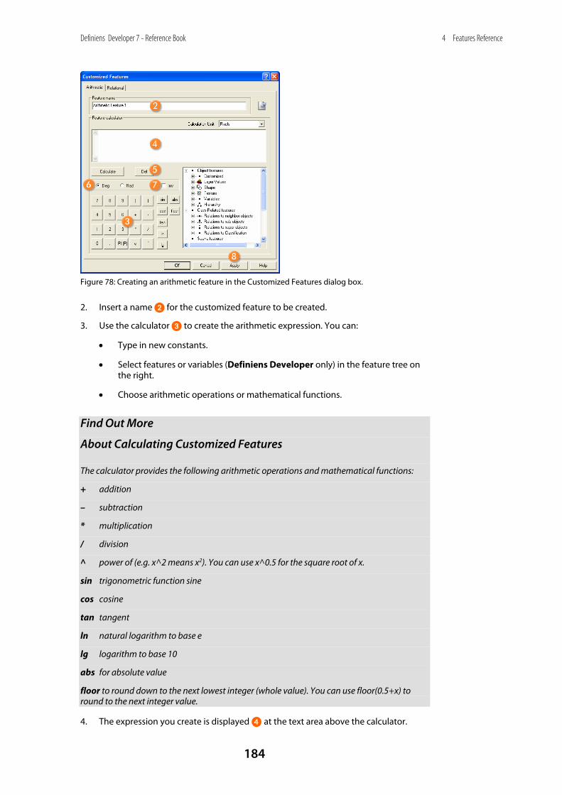
Definiens Developer 7 - Reference Book
184
4 Features Reference
Figure 78: Creating an arithmetic feature in the Customized Features dialog box.
2. Insert a name O for the customized feature to be created.
3. Use the calculator P to create the arithmetic expression. You can:
• Type in new constants.
• Select features or variables (Definiens Developer only) in the feature tree on the right.
• Choose arithmetic operations or mathematical functions.
Find Out More
About Calculating Customized Features
The calculator provides the following arithmetic operations and mathematical functions:
+ addition
– subtraction
* multiplication
/ division
^ power of (e.g. x^2 means x2). You can use x^0.5 for the square root of x.
sin trigonometric function sine
cos cosine
tan tangent
ln natural logarithm to base e
lg logarithm to base 10
abs for absolute value
floor to round down to the next lowest integer (whole value). You can use floor(0.5+x) to round to the next integer value.
4. The expression you create is displayed Q at the text area above the calculator.
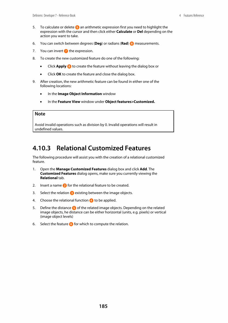
Definiens Developer 7 - Reference Book
185
4 Features Reference
5. To calculate or delete R an arithmetic expression first you need to highlight the expression with the cursor and then click either Calculate or Del depending on the action you want to take.
6. You can switch between degrees (Deg) or radians (Rad) S measurements.
7. You can invert T the expression.
8. To create the new customized feature do one of the following:
• Click Apply U to create the feature without leaving the dialog box or
• Click OK to create the feature and close the dialog box.
9. After creation, the new arithmetic feature can be found in either one of the following locations:
• In the Image Object Information window
• In the Feature View window under Object features>Customized.
Note
Avoid invalid operations such as division by 0. Invalid operations will result in undefined values.
4.10.3 Relational Customized Features The following procedure will assist you with the creation of a relational customized feature.
1. Open the Manage Customized Features dialog box and click Add. The Customized Features dialog opens, make sure you currently viewing the Relational tab.
2. Insert a name O for the relational feature to be created.
3. Select the relation P existing between the image objects.
4. Choose the relational function Q to be applied.
5. Define the distance R of the related image objects. Depending on the related image objects, he distance can be either horizontal (units, e.g. pixels) or vertical (image object levels)
6. Select the feature S for which to compute the relation.
Definiens Developer 7 - Reference Book
186
4 Features Reference
Figure 79: Creating a relational feature at the Customized Features dialog box.
7. Select a class, a group or no class T to apply the relation.
8. To create the new customized feature do one of the following:
• Click Apply U to create the feature without leaving the dialog box or
• Click OK to create the feature and close the dialog box.
9. After creation, the new relational feature can be found in the Feature View window under Class-Related features > Customized.
Note
As with class-related features, the relations refer to the groups hierarchy. This means if a relation refers to one class, it automatically refers to all subclasses of this class in the groups hierarchy.
Relations between surrounding objects can exist either on the same level or on a level lower or higher in the image object hierarchy:
neighbors Related image objects on the same level. If the distance of the image objects is set to 0 then only the direct neighbors are considered. When the distance is greater than 0 then the relation of the objects is computed using their centers of gravity. Only those neighbors whose center of gravity is closer than the distance specified from the starting image object are considered. The distance is calculated either in metric units or pixels. For example, a direct neighbor might be ignored if its center of gravity is further away from the specified distance.
subobjects Image objects that exist under other image objects (superobjects) whose position in the hierarchy is higher. The distance is calculated in levels.
superobject Contains other image objects (subobjects) on lower levels in the hierarchy. The distance is calculated in levels.
Definiens Developer 7 - Reference Book
187
4 Features Reference
sub-objects of superobject Only the image objects that exist under a specific super-object are considered in this case. The distance is calculated in levels.
level Specifies the level on which an image object will be compared to all other image objects existing at this level. The distance is calculated in levels.
The following table gives an overview of all functions existing in the drop-down list under the Relational function section:
Mean Calculates the mean value of selected features of an image object and its neighbors. You can select a class to apply this feature or no class if you want to apply it to all image objects.
Standard deviation Calculates the standard deviation of selected features of an image object and its neighbors. You can select a class to apply this feature or no class if you want to apply it to all image objects.
Mean difference Calculates the mean difference between the feature value of an image object and its neighbors of a selected class. Note that for averaging, the feature values are weighted by the size of the respective objects.
Mean absolute difference Calculates the mean absolute difference between the feature value of an object and the feature values of its neighbors of a selected class. Note that for averaging, the absolute difference to each neighbor is weighted by the respective size.
Ratio Calculates the proportion between the feature value of an image object and the mean feature value of its neighbors of a selected class. Note that for averaging the feature values are weighted with the size of the corresponding image objects.
Sum Calculates the sum of the feature values of the neighbors of a selected class.
Number Calculates the number of neighbors of a selected class. The feature you have selected is of no account. But it has to be selected for working of the feature.
Min Returns the minimum value of the feature values of an image object and its neighbors of a selected class.
Max Returns the minimum value of the feature values of an image object and its neighbors of a selected class.
Mean difference to higher values
Calculates the mean difference between the feature value of an image object and the feature values of its neighbors of a selected class, which have higher values than the image object itself. Note that for averaging the feature values are weighted by the size of respective image objects.
Mean difference to lower values
Calculates the mean difference between the feature value of an image object and the feature values of its neighbors of a selected class, which have lower values than the object itself. Note that for averaging the feature values are weighted by the size of the respective image objects.
Portion of higher value area Calculates the portion of the area of the neighbors of a selected class, which have higher values for the specified feature than the object itself to the area of all neighbors of the selected class.
Portion of lower value area Calculates the portion of the area of the neighbors of a selected class, which have lower values for the specified feature than the object itself to the area of all neighbors of the selected class.
Definiens Developer 7 - Reference Book
188
4 Features Reference
Portion of higher values Calculates the feature value difference between an image object and its neighbors of a selected class with higher feature values than the object itself divided by the difference of the image object and all its neighbors of the selected class. Note that the features are weighted with the size of the corresponding image objects.
Portion of lower values Calculates the feature value difference between an image object and its neighbors of a selected class with lower feature values than the object itself divided by the difference of the image object and all its neighbors of the selected class. Note that the features are weighted with the size of the corresponding image object.
4.11 Use Variables as Features The following variables can be used as features:
• Scene variables
• Object variables
• Feature variables
They display in the feature tree of for example the Feature View window or the Select Displayed Features dialog box.
4.12 About Metadata as a Source of Information
Many image data formats include metadata providing information about the related image, for example the acquisition time. Considering metadata might be beneficial for image analysis if you relate it to features.
The available metadata depends on the image reader or camera used, the industry-specific environment, and settings. Industry-specific examples are:
• Satellite image data may contain metadata providing cloudiness information.
• Microscopy image data may contain metadata providing information about the used magnification.
Definiens Developer can provide a selection of the available metadata. This selection is defined in a metadata definition which is part of the rule set.
The provided metadata can be displayed in the Image Object Information window. Further, it is listed together with features and variables in the feature tree of for example the Feature View window or the Select Displayed Features dialog box.
Use Variables section of the User Guide
Variables on page 173
Variables on page 160
Feature Variables on page 182
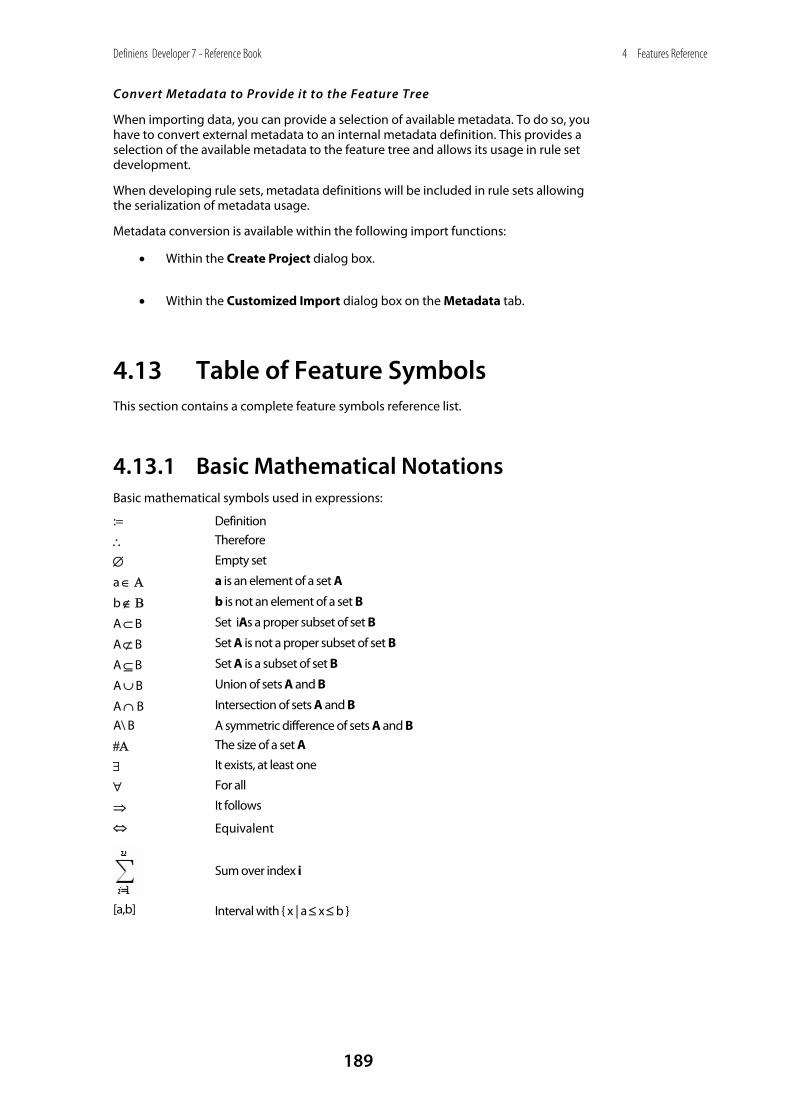
Definiens Developer 7 - Reference Book
189
4 Features Reference
Convert Metadata to Provide it to the Feature Tree
When importing data, you can provide a selection of available metadata. To do so, you have to convert external metadata to an internal metadata definition. This provides a selection of the available metadata to the feature tree and allows its usage in rule set development.
When developing rule sets, metadata definitions will be included in rule sets allowing the serialization of metadata usage.
Metadata conversion is available within the following import functions:
• Within the Create Project dialog box.
• Within the Customized Import dialog box on the Metadata tab.
4.13 Table of Feature Symbols This section contains a complete feature symbols reference list.
4.13.1 Basic Mathematical Notations Basic mathematical symbols used in expressions:
:= Definition
∴ Therefore
∅ Empty set
a ∈ Α a is an element of a set A
b ∉ Β b is not an element of a set B
A ⊂ B Set iAs a proper subset of set B
A ⊄ B Set A is not a proper subset of set B
A ⊆ B Set A is a subset of set B
A ∪ B Union of sets A and B
A ∩ B Intersection of sets A and B
A\ B A symmetric difference of sets A and B
#Α The size of a set A
∃ It exists, at least one
∀ For all
⇒ It follows
⇔ Equivalent
Sum over index i
[a,b] Interval with { x | a ≤ x ≤ b }
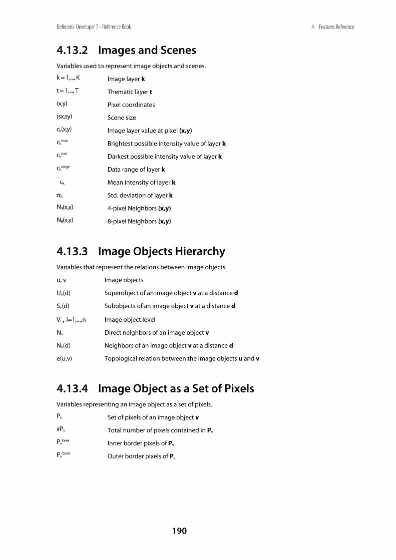
Definiens Developer 7 - Reference Book
190
4 Features Reference
4.13.2 Images and Scenes Variables used to represent image objects and scenes.
k = 1,..., K Image layer k
t = 1,..., T Thematic layer t
(x,y) Pixel coordinates
(sx,sy) Scene size
ck(x,y) Image layer value at pixel (x,y)
ckmax Brightest possible intensity value of layer k
ckmin Darkest possible intensity value of layer k
ckrange Data range of layer k
⎯ck Mean intensity of layer k
σk Std. deviation of layer k
N4(x,y) 4-pixel Neighbors (x,y)
N8(x,y) 8-pixel Neighbors (x,y)
4.13.3 Image Objects Hierarchy Variables that represent the relations between image objects.
u, v Image objects
Uv(d) Superobject of an image object v at a distance d
Sv(d) Subobjects of an image object v at a distance d
Vi , i=1,...,n Image object level
Nv Direct neighbors of an image object v
Nv(d) Neighbors of an image object v at a distance d
e(u,v) Topological relation between the image objects u and v
4.13.4 Image Object as a Set of Pixels Variables representing an image object as a set of pixels.
Pv Set of pixels of an image object v
#Pv Total number of pixels contained in Pv
PvInner Inner border pixels of Pv
PvOuter Outer border pixels of Pv
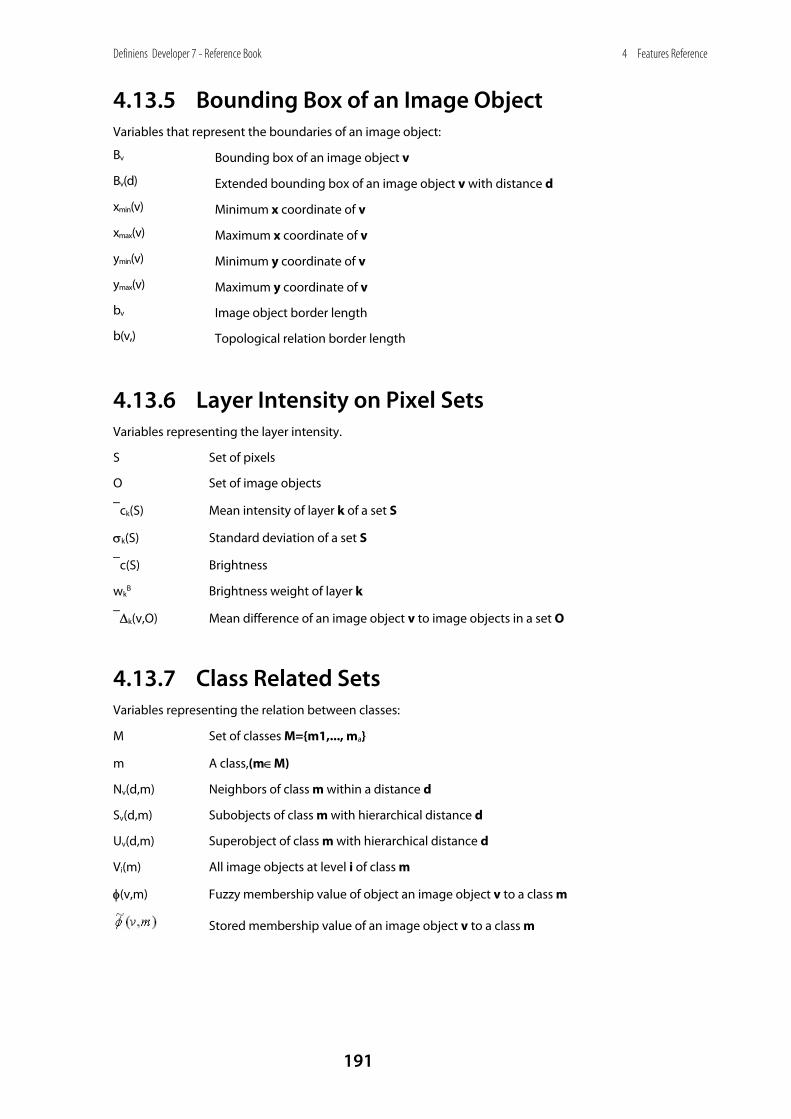
Definiens Developer 7 - Reference Book
191
4 Features Reference
4.13.5 Bounding Box of an Image Object Variables that represent the boundaries of an image object:
Bv Bounding box of an image object v
Bv(d) Extended bounding box of an image object v with distance d
xmin(v) Minimum x coordinate of v
xmax(v) Maximum x coordinate of v
ymin(v) Minimum y coordinate of v
ymax(v) Maximum y coordinate of v
bv Image object border length
b(v,) Topological relation border length
4.13.6 Layer Intensity on Pixel Sets Variables representing the layer intensity.
S Set of pixels
O Set of image objects
⎯ck(S) Mean intensity of layer k of a set S
σk(S) Standard deviation of a set S
⎯c(S) Brightness
wkB Brightness weight of layer k
⎯Δk(v,O) Mean difference of an image object v to image objects in a set O
4.13.7 Class Related Sets Variables representing the relation between classes:
M Set of classes M={m1,..., ma}
m A class,(m∈M)
Nv(d,m) Neighbors of class m within a distance d
Sv(d,m) Subobjects of class m with hierarchical distance d
Uv(d,m) Superobject of class m with hierarchical distance d
Vi(m) All image objects at level i of class m
φ(v,m) Fuzzy membership value of object an image object v to a class m
Stored membership value of an image object v to a class m
Definiens Developer 7 - Reference Book
192
5 Index
5 Index A apply parameter set 40 Area 115 Area (excluding inner polygons) 140 Area (including inner polygons) 140 Area of 168 Area of classified objects 173 Area of subobjects
mean 148 arithmetic customized feature 183 assign class 28 Asymmetry 115 Asymmetry of subobjects
mean 150 stddev. 150
Average branch length 143 Average length of branches of order
143 Average length of edges (polygon)
141 Avrg. area represented by segments
144 Avrg. mean diff. to neighbors of
subobjects 147
B Based on Polygons 139 Based on Skeletons 142 Border index 116 Border length 117 border optimization 46 Border to 164 bounding box 90, 191 Brightness 97
C calculate brightness from layers 97 candidate 43 Chessboard segmentaion 15 Clark Aggregation Index 169 classification 28
classification algorithms 28, 29 Classification value of 171 Classified as 171 classified image objects to samples 54 Class-related 173 Class-Related Features 91, 163 cleanup redundant samples 55 closing 47 color space transformation 113 Compactness 117 Compactness (polygon) 141 compactness criteria 21 composition of homogeneity 21 compute statistical value 39 configure object table 52 connector 34 contrast filter segmentation 25 Contrast to neighbor pixels 103
convert to subobjects 46 coordinates 93 copy image object level 49 create scene copy 74 create scene subset 75 create scene tiles 78 create temporary image layer 56 create/modify project 50 Curvature/length (line so) 126 Curvature/length (only main line) 144 customized feature 96, 163, 179, 182
arithmetic 183 create 182 relational 185
D Degree of skeleton branching 144 delete all samples 55 delete all samples of class 55 delete image layer 56 delete image object level 50 delete scenes 80 Density 118 Density of subobjects
mean 149 stddev. 149
diff. PPO 178 Direction of subobjects
mean 151 stddev. 152
disconnect all samples 55 display image object level 52 Distance to 167 Distance to image border 128 Distance to line 128 Distance to superobject center 137 distance-related features 94 duplicate image object level 49
E Edges longer than 139 edit image layer mix 7 Elliptic Dist. from PPO 180 Elliptic distance to superobject center
137 Elliptic fit 118 equalization 7 execute child process 13 Existence of 164, 168, 170 Existence of image layers 175 Existence of object level 175 Existence of thematic layers 176 export algorithms 67 export classification view 68 export current view 68 export domain statictics 70 export object statistics 72 export object statistics for report 72 export project statistics 71 export thematic raster files 70 export vector layers 73
Definiens Developer 7 - Reference Book
193
5 Index
F feature 83
customized feature 96, 163, 179, 182
distance 87 value conversion 84
find domain extrema 30 find enclosed by class 33 find enclosed by image object 33 find local extrema 31 fusion See image object 43
G gamma correction 8 Generic 115 GLCM ang. 2nd moment 156 GLCM contrast 154 GLCM correlation 158 GLCM dissimilarity 155 GLCM entropy 155 GLCM homogeneity 154 GLCM mean 156 GLCM stddev. 157 GLDV angular 2nd moment 158 GLDV contrast 159 GLDV entropy 158 GLDV mean 159 global feature 83 global variable - See scene variable
173 grow region 41
H hierarchal classification 29 hierarchical distance 87 hierarchy 161 histogram 8 HSI color space transformation 113 Hue 113
I image
equalization 8 image layer
equalization 7 operation 56 related features 84
image object related features 87
image object fusion 43 image object hierarchy 87 Image size X 177 Image size Y 177 Intensity 114 interactive operation algorithms 50 Is center of superobject 138 Is end of superobject 138
L Largest actual pixel value 176 Layer mean of classified objects 174 Layer stddev. of classified objects 174
Layer Value Texture Based on Subobjects 147
Layer Values 96 Length 119 Length (line so) 126 Length of longest edge (polygon) 141 Length of main line (no cycles) 144 Length of main line (regarding cycles)
145 Length/Width 119 Length/width (line so) 125 Length/width (only main line) 145 level 161
level distance 88 level operation algorithms 49 Line Features Based on Subobject
Analysis 125 local variable 160
M Main direction 120 Manual Classification 52 Max. diff. 98 Max. pixel value 101 Maximum branch length 145 Mean 96 Mean diff. to 167 Mean diff. to brighter neighbors 108 Mean diff. to darker neighbors 107 Mean diff. to neighbors 104 Mean diff. to neighbors (abs) 106 Mean diff. to scene 112 Mean diff. to superobject 109 Mean of inner border 102 Mean of outer border 102 Mean of scene 176 Mean of subobjects
stddev. 147 Membership to 171 merge region 40 merge results back to the main scene
78, 80 metadata 188 Min. pixel value 100 morphology 47 multiresolution segmentation 21 multiresolution segmentation region
grow 42
N nearest neighbor configuration 55 Number of 164, 168 Number of branches of length 143 Number of branches of order 143 Number of classified objects 173 Number of edges (polygon) 141 Number of higher levels 161 Number of inner objects (polygon) 141 Number of layers 177 Number of neighbors 161 Number of objects 177 Number of overlapping thematic
objects 163

Definiens Developer 7 - Reference Book
194
5 Index
Number of pixels 177 Number of right angles with edges
longer than 139 Number of samples 178 Number of samples per class 173 Number of segments 145 Number of segments of order 143 Number of sublevels 162 Number of subobjects 162 Number of thematic layers 178
O Object Features 95 opening 47
P Perimeter (polygon) 141 Pixel Based 100 Pixel resolution 178 Position 128 position value 84 process related algorithms 13 process-related feature 178
Q quad tree based segmentaion 16
R Radius of largest enclosed ellipse 121 Radius of smallest enclosing ellipse
122 Ratio 100 ratio PPO 179 Ratio to scene 112 Ratio to superobject 110 read subscene statistics 80 read thematic attributes 67 Rectangular fit 122 Rel. area of 166, 169 Rel. area to superobject 135 Rel. border to 165 Rel. border to brighter neighbors 109 Rel. border to PPO 180 Rel. inner border to superobject (n)
136 Rel. rad. position to superobject (n)
135 relational customized feature 185 Relations to Classification 171 Relations to Neighbor Objects 164 Relations to Subobjects 168 remove objects 40 rename image object level 50 rescaling 68, 74, 75 reshaping operation algorithms 40 result summary 80 Roundness 123
S Same superobject as PPO 180 sample operation algorithms 54 sample selection 56 Saturation 114 scale
rescaling 68, 74, 75 scale parameter 21 scene 84
scene feature 173 scene variable 173
scene variable 173 Scene-related 177 seed 43 segmentation algorithms 15 select input mode 53 Shape 115 shape criteria 21 Shape index 124 Shape Texture Based on Subobjects
148 shape-related features 91 show user warning 50 Smallest actual pixel value 176 spatial distance 89 spectrail difference segmentaion 24 Standard deviation 84, 99 std. deviation to neighbor pixels 104 Stddev of length of edges 142 Stddev. 176 Stddev. curvature (line so) 127 Stddev. curvature (only main line) 145 Stddev. diff. to superobject 111 Stddev. of area represented by
segments 146 Stddev. Ratio to superobject 111 stitching results 78 submit scenes for analysis 78 subroutine 74 sycronize image object hierarchy 67
T target 43 Texture 146 Texture After Haralick 152 Thematic Attributes 163 thematic layer operation algorithms
66 Thematic object ID 163 thematic objects attribute 163 tiling 78 To Neighbors 104 To Scene 112 To Superobject 109, 135 training operation algorithms 50
U unit
conversion of 85 update action from parameter set 51 update parameter set from action 52 update variable 37
V value conversion 84 variable 188
scene variable 173 update variable 37
variables operation algorithms 37

Definiens Developer 7 - Reference Book
195
5 Index
vectorization 54
W watershed transformation 49 Width 124 Width (line so) 125 Width (only main line) 146 workspace automation 74 write thematic attributes 67
X X center 129 X distance to image left border 130 X distance to image right border 130 X max. 131 X min. 131
Y Y center 132 Y distance to image bottom border
133 Y distance to image top border 134 Y max. 132 Y min. 133