DEFINING HABITAT FOR THE RECOVERY OF

OCELOTS (LEOPARDUS PARDALIS)

IN THE UNITED STATES

THESIS

Presented to the Graduate Council of

Texas State University-San Marcos

in Partial Fulfillment

of the Requirements

for the Degree

Master of SCIENCE

by

Amy Rosamond Connolly, B.S.

San Marcos, Texas

December 2009

DEFINING HABITAT FOR THE RECOVERY OF

OCELOTS (LEOPARDUS PARDALIS)

IN THE UNITED STATES

Committee Members Approved

______________________________

Thomas R. Simpson, Chair

______________________________

M. Clay Green

______________________________

John Young

Approved:

______________________________

J. Michael Willoughby

Dean of the Graduate College

COPYRIGHT

by

Amy Rosamond Connolly

2009

iv

ACKNOWLEDGMENTS

This project was funded by a Section 6 Endangered Species Grant offered by the

United States Fish and Wildlife Service and Texas Parks and Wildlife with a match from

Texas State University-San Marcos. The U.S.F.W.S. has some brilliant people that

helped me along, including Jody Mays, Wendy Brown and Mitch Sternberg.

I can’t thank Dr. Thomas R. Simpson enough for giving me the inspiration and

wisdom to be a wildlife biologist, as well as being my advisor for this project. I thank Dr.

M. Clay Green and Dr. John Young for being committee members on this project as well

as giving me advice on every other thing I can think of. Dr. F. Weckerly and Dr. T.

Bonner were my statistical gurus in this project. This project couldn’t have been done

without the help of all the landowners Steve Bentsen, Sylvia Chavez, Jim and Kathy

Collins, Randy Fugate, Felo and Luis Guerra, Jim McAllen, and other landowners who

wish to remain anonymous, that gave us their trust and access to their property. They

truly are our only hope for a better world. I wouldn’t have been able to keep my senses if

it weren’t for all my assistants (Natalie Uriarte, Chris Willy, Jacquie Ferrato, Eric Lee,

and Romey Swanson) that slaved away with me in the field through thick and thicker

with smiles on their faces. Of course, I thank my friends and family for being completely

understanding and supportive through all of my crazy days for the past two years. Most

importantly, if you met me at any point during this project or beforehand, just know that I

remember you and I am grateful for your help and influence.

This manuscript was submitted on November 10, 2009.

v

TABLE OF CONTENTS

Page

ACKNOWLEDGMENTS ................................................................................................. iv

LIST OF TABLES ............................................................................................................. vi

LIST OF FIGURES .......................................................................................................... vii

ABSTRACT ..................................................................................................................... viii

CHAPTER

I. INTRODUCTION ............................................................................................................1

II. STUDY AREA ................................................................................................................5

III. METHODS

COVER MAP ..........................................................................................................8

FIELD METHODS ................................................................................................11

IV. RESULTS ....................................................................................................................14

V. DISCUSSION ...............................................................................................................25

VI. MANAGEMENT IMPLICATIONS ...........................................................................28

APPENDIX: C-CAP DESCRIPTIONS OF LAND-USE/LAND-COVER CLASSES ....31

LITERATURE CITED ......................................................................................................33

vi

LIST OF TABLES

Table Page

1. Land-use types preferred/avoided by ocelots ................................................................10

2. Soils preferred and avoided by ocelots ..........................................................................14

3. Number of woody species throughout South Texas sites ..............................................15

4. Means of habitat components from all transects on each site ........................................17

vii

LIST OF FIGURES

Figure Page

1. Map of Laguna Atascosa National Wildlife Refuge ........................................................5

2. Map of all study sites across S. Texas overlaid on C-CAP shrub/scrub classification ....6

3. Radio-telemetry points overlaid on top of C-CAP land-cover layer ...............................9

4. VPB for LANWR vs. Other ...........................................................................................18

5. VPB for LANWR vs. FWS ............................................................................................19

6. VPB comparing sites east-west ......................................................................................20

7. PCA biplot of all transects .............................................................................................21

8. PCA for LANWR vs. FWS ............................................................................................22

9. PCA for sites east-west .................................................................................................22

10. PCA comparing individual sites with scatterplot........................................................24

11. Shrub/scrub cover map for South Texas produced by Sternberg (FWS, 2009)...........29

viii

ABSTRACT

DEFINING HABITAT FOR RECOVERY OF

OCELOTS (LEOPARDUS PARDALIS)

IN THE UNITED STATES

by

Amy Rosamond Connolly, B.S.

Texas State University-San Marcos

December 2009

SUPERVISING PROFESSOR: THOMAS R. SIMPSON

The ocelot (Leopardus pardalis) was placed on the United States federal

endangered species list in 1982. Historically these felids were hunted for their pelts, but

other factors have contributed over the years to their placement on the list. Today, the

major factor that causes ocelots to be endangered is loss of habitat. Previous research has

demonstrated that ocelots prefer habitats of dense shrubs with greater than 95% canopy

cover. However, little else is known about the total composition of vegetation in their

habitat. The objectives of our study were to develop a geographic information system

ix

(GIS) containing vegetation, soil and satellite imagery for seven counties (Willacy,

Cameron (Laguna Atascosa National Wildlife Refuge), Starr, Hidalgo, Jim Hogg,

Kenedy, and Zapata) in South Texas to enhance prior research and define areas suitable

to support ocelots. Ground-truthing on vegetation transects on public and private land

across these counties was performed using a densiometer, vegetation profile board

(VPB), and Daubenmire frame techniques to determine key vegetative characteristics that

comprise ocelot habitat. Through principal components analysis (PCA), we analyzed

slope and intercept (VPB measures), percent canopy cover (overstory), percent grass,

litter, bare ground, and forbs from Daubenmire frames, woody species richness, woody

plant density, woody plant diversity, and average woody plant height per transect. We

found the majority of ocelot habitat was characterized by greater plant diversity, greater

vertical cover density at ground level, greater canopy cover, smaller shrubs, and more

ground litter than habitat not occupied by ocelots. Along an east-west gradient in South

Texas, eastern sites were more similar to ocelot habitat. Comprehensive vegetation

information (i.e. plant density, percent grass, etc.) is lacking on satellite/ land-use images.

Therefore, comparing habitat data through PCA analysis would be more effective in

delineating ocelot habitat.

1

CHAPTER I

INTRODUCTION

The ocelot (Leopardus pardalis) was listed by the United States Fish and Wildlife

Service (USFWS) as a federally endangered species in 1982. Historically these spotted

cats were hunted for their pelts, and subjected to predator control due to perceived

competition for livestock and game (Broad 1987). However, the major cause for decline

in ocelot populations in the U.S is loss of habitat (Murray and Gardner 1997). During the

1800s ocelots ranged from Peru and Argentina, northward to Arizona, Texas, Louisiana

and Arkansas in the United States (Haines, et al. 2006). Today, only an estimated 30-100

ocelots remain in the United States (Laack, et al. 2005) on the Yturria Ranch and Laguna

Atascosa National Wildlife Refuge (LANWR) in Willacy and Cameron County in South

Texas. Outside of the United States, ocelots inhabit a wide variety of ecosystems,

including swamps, marshes, grasslands, tropical-humid forests, and evergreen forests, but

their movement patterns indicate that they are strongly associated with dense forests,

suggesting that they are habitat specialists (Murray and Gardner 1997). A comparison of

ocelots and bobcats (a felid similar in size and life history) showed that ocelots selected

areas with more closed cover while bobcats favored mixed and open cover (Horne et al.

2009). Ocelots also required areas with high rodent density (Emmons 1988), further

justifying the habitat specialist theory. The principle habitat in which the majority of

2

ocelots are found in the United States is dense thorny chaparral of the Rio Grande Valley,

also known as Tamaulipan Thorn Scrub (Schmidly 1977). Over 95% of ocelot habitat has

been converted to agricultural and residential uses (Shindle and Tewes 1998).

Consequently there is little Tamaulipan Thorn Scrub habitat between Yturria Ranch and

LANWR, and the remaining habitat is extremely fragmented. A recent habitat population

viability analysis concluded that the best plan for ocelot survival would be one that

included reduction of road mortality, translocation and habitat restoration (Haines 2006a).

Based on a recent telemetry study, a habitat suitability regression was performed,

and found that ocelots inhabited areas with or adjacent to closed canopy, and ocelots

were furthest from areas with open cover/bare ground (Haines et al. 2005). Ocelots have

also been found to select habitat with >95% horizontal cover and avoid habitat with

<75% cover (Harveson et al. 2004). A species-type analysis was performed for all woody

species >0.5m tall and granjeno (Celtis pallida), brasil (Condalia hookeri), crucita

(Eupatorium odoratum), colima (Zanthoxylum fagara), whitebrush (Alloysia gratissima),

lotebush (Zizyphus obtusifolia), and desert olive (Forestiera angustifolia) were common

in ocelot territories (Shindle and Tewes 1998). Ocelots also prefer medium-sized areas

with closed canopy, avoid small areas of this habitat type, and avoid large areas of open

canopy (Jackson et al. 2005).

In order for certain types of vegetation to grow, specific soil types must be

present. Harveson et al. (2004) determined that ocelots select habitat with four soil types

(Camargo, Laredo, Olmito, and Point Isabel) and avoid 11 types (Barrada, Benito,

Delfina, Harlingen, Latina, Lyford, Raymondville, Sejita, Willacy, Willamar, and Other).

3

In agreement with vegetative studies of habitat selection, ocelots selected for 82% of the

soil series found in dense cover (Harveson et al. 2004).

Modelling with GIS will assist in identifying relocation sites that contain suitable

habitat. Spatial habitat analysis using GIS can identify necessary core areas that will have

a level of protection sufficient to buffer populations against human-caused mortality

(Carroll et al. 2001). Habitat components including road density (increases mortality),

soil structure, canopy cover, and home range can be used as layers for such a model. A

recent study done in 2003 found ocelot density in the Pantanal to be 2.82 individuals per

5 km2 (Trolle and Kery 2003).

Estimated home range size in Texas was 1.56 km

2. Based

on a RAMAS/gis spatial data model, 11 habitat patches were identified in Texas with an

area greater than 3.71 km2, which was deemed large enough to potentially support at least

one breeding male ocelot per patch, but overall could only support a total carrying

capacity of 82 ocelots (Haines et al. 2005). In addition to home range, many other

variables need to be considered such as prey density, the vegetation structure of

reproductive dens, and herbaceous species. Little, if anything, is known about these

components for ocelots in the United States. For recovery of any species, many habitat

requirements need to be known in order to provide the best chances for survival.

A few studies have acknowledged the importance of vegetation (Shindle and

Tewes 1998, Young and Tewes 2004, Laack et al. 2005) for ocelots, however little is

known about vegetative structure. The objectives of our study were to a) gather spatial

data of vegetation and soil characteristics using satellite imagery and available GIS layers

for seven counties (Willacy, Cameron, Starr, Hidalgo, Jim Hogg, Kenedy, and Zapata) to

expand on prior research (Shindle et al. 1998, Harveson et al. 2004, Sternberg and

4

Donnelly, USFWS, in review) for defining existing habitat suitable to support an ocelot

population of 200 individuals in Texas (USFWS, 2006), b) assess vegetative components

of habitat currently occupied by ocelots in South Texas, adding additional habitat

parameters (vertical structure of woody vegetation, herbaceous ground cover, etc.)

beyond those currently defined in the literature and, c) “ground-truth” selected sites based

on available GIS layers and satellite imagery. Our objectives would help fulfill the first

goal of the USFWS’ Plan for Translocation of Northern Ocelots to “assess sufficient

habitat… to support viable populations of the ocelot in the borderlands of the U.S. and

Mexico” (USFWS Translocation Team, 2009).

5

CHAPTER II

STUDY AREA

We collected vegetative data from known ocelot habitat on Laguna Atascosa

National Wildlife Refuge (LANWR) in Cameron County, Texas (Fig. 1).

Figure 1. Map of Laguna Atascosa National Wildlife Refuge

6

The refuge consists of 18,287 hectares with multiple management techniques for

wintering migrating birds and re-establishing native brushlands on land converted for

agricultural practices. Typical vegetation at LANWR is dominated by Tamaulipan Thorn

Scrub, including species such as honey mesquite (Prosopis glandulosa), prickly pear

(Opuntia lindheimeri) and persimmon (Diospyros virginiana). The climate is temperate

and subtropical with mean annual precipitation of 19 cm and an average daily

temperature of 13C.

Defining and evaluating potential ocelot habitat was conducted on nine sites

across South Texas along an east-west line in Willacy (three sites), Hidalgo (two sites),

Brooks (one site), and Starr (two sites) counties (Fig. 2), approximately 60 km north of

the Lower Rio Grande Valley.

Figure 2. Map of all study sites across S. Texas overlaid on C-CAP shrub/scrub

classification

7

Sites ranged in size from 81 to 12,141 ha with land management ranging from

conservation/ecotourism to agriculture/cattle. Three sites were owned by United States

Fish and Wildlife Service (USFWS) (two containing ocelots). Seven sites were located

on privately-owned ranches with no known occurrences of ocelots. This area contains

Tamaulipan Thorn Scrub mixed in a grassland ecosystem (Bezanson 2001). Soil types

included sands, clays, loams, and caliche, with some saline, alkaline, and gypseous soils

(Bezanson 2001).

8

CHAPTER III

METHODS

COVER MAP

I downloaded the Texas 2005 land cover maps from Coastal Change Analysis

Program (C-CAP) created by the National Oceanic and Atmospheric Administration

Coastal Services Center. (http://www.csc.noaa.gov, 11/2009). I chose C-CAP data over

other readily obtainable databases (i.e. TX-GAP) for two reasons. First, the satellite

images are classified into distinctive subcategories such as palustrine aquatic bed,

deciduous forest, low intensity developed (Appendix A), whereas other land cover maps

are classified only into major categories such as water, forest, and developed. Both

supervised and unsupervised classification techniques were used to create their images.

Second, C-CAP has the only land cover map that has an overall target accuracy of 85

percent, which is verified through field assessment. This meets the minimum standard for

classification criteria needed for management and planning purposes (Anderson et al.

1976).

Ocelot telemetry points (unpublished data, USFWS, 1991 – 2005) were overlaid

on the land cover layer using arcMAP (Environmental Systems Research Institute,

Version 9.3) (Fig. 3).

9

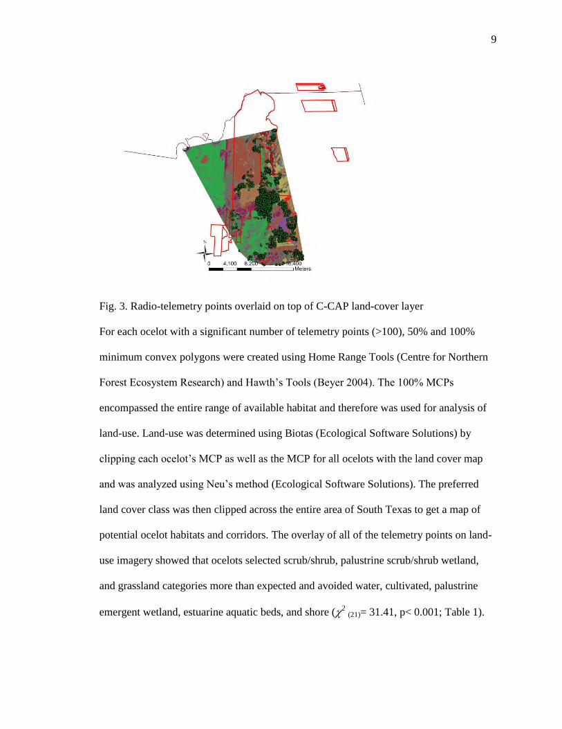
Fig. 3. Radio-telemetry points overlaid on top of C-CAP land-cover layer

For each ocelot with a significant number of telemetry points (>100), 50% and 100%

minimum convex polygons were created using Home Range Tools (Centre for Northern

Forest Ecosystem Research) and Hawth’s Tools (Beyer 2004). The 100% MCPs

encompassed the entire range of available habitat and therefore was used for analysis of

land-use. Land-use was determined using Biotas (Ecological Software Solutions) by

clipping each ocelot’s MCP as well as the MCP for all ocelots with the land cover map

and was analyzed using Neu’s method (Ecological Software Solutions). The preferred

land cover class was then clipped across the entire area of South Texas to get a map of

potential ocelot habitats and corridors. The overlay of all of the telemetry points on land-

use imagery showed that ocelots selected scrub/shrub, palustrine scrub/shrub wetland,

and grassland categories more than expected and avoided water, cultivated, palustrine

emergent wetland, estuarine aquatic beds, and shore (2 (21)= 31.41, p< 0.001; Table 1).

10

Table 1. Land-use types preferred/avoided by ocelots

Land-use Type Observed Count Expected Use

Evergreen forest 2 6

Mixed forest 2 4

shrub/scrub* 6602 2280

Palustrine forested wetland 125 101

Palustrine shrub/scrub* 2358 779

Palustrine emergent wetland* 1956 3549

Estuarine shrub/scrub 0 1

Estuarine emergent wetland 34 153

Unconsolidated shore* 467 1136

High intensity developed 3 6

Bare 46 182

Water* 170 1073

Palustrine aquatic bed 14 50

Estuarine aquatic bed* 17 416

Medium intensity developed 53 129

Low intensity developed 639 358

Developed open space 100 167

Cultivated* 494 3974

Pasture/Hay 36 107

Grassland* 2984 1756

Deciduous Forest 212 88 * represents p<.001

I initially defined the three selected categories as “suitable” categories, but when

extrapolated across South Texas, these categories resulted in resolution too coarse for

habitat suitability. For a more clearly defined habitat suitability map, I chose the

shrub/scrub category to identify usable potential habitat more specifically (Fig. 2).

Soil classification was also determined using Biotas and analyzed using Neu’s

method (Ecological Software Solutions). Soil data were obtained from National Resource

Conservation Service Soil Data Mart. Neu’s method allowed for analysis of

observed/expected use. The method was performed on the ocelot habitat at LANWR and

then compared with soil types on all vegetation transects.

11

FIELD METHODS

Analysis of current ocelot habitat was conducted on LANWR in Cameron

County, Texas. Using Hawth’s Tools, I randomly chose 30 telemetry points from areas

that were travelled frequently by multiple ocelots from 1990-2005. I ground-truthed each

point by measuring vegetation parameters along 50-meter transects. Azimuth of each

transect was randomly chosen using the statistical program R (R development core team

2005).

Along each transect I measured canopy cover and abundance of woody species

using line-intercept method. I recorded an additional measure of canopy cover every 10

m using a bull-horn densiometer (Geographic Resources Solutions, Arcata, California),

taken at 1m height, sufficient height to provide cover for an ocelot. Vertical screening

cover was measured at 0, 25, and 50 m along each transect using a vegetation profile

board (VPB) (Nudds 1977). The board was placed 10 m in both directions perpendicular

from the transect. Generally at distances > 10 m, vegetation obscured the board

completely. Percentages of forbs, grasses, bare ground, and litter were measured every 10

m using a Daubenmire frame (Daubenmire 1959). Density of woody vegetation was

measured every 10 m using the point center quarter method (Bryant, et al. 2004).

I analyzed vegetation baseline data (i.e. means, abundances, etc.) using program R

(R Development Core Team, 2005) and Excel (Microsoft Corporation, Redmond,

Washington). Analysis of VPB data was performed in Excel by calculating the mean

percent vertical vegetative obstruction (VVO) for each 0.5 m vertical section of the board

for each transect and calculating a linear regression equation for means for each 0.5 m

vertical section. The y-intercept represents the mean percent VVO for section 1 (ground

12

level, where ocelots reside), and the slope represents the mean change in percent VVO

for each section on the board. An ANCOVA type III sums of squares was used to test for

any correlation between the type of habitat and the sections of the VPB. T-tests were used

to determine similarities in woody species between transects. I calculated mean density

measurements per transect. Simpson’s index (D) was used to determine diversity for each

transect.

Vegetative measurements on private lands across South Texas were done in the

same manner as the analysis of current ocelot habitat, using the same vegetation

parameters. We recorded vegetative data from at least one transect per 1500 acres, the

same amount performed at LANWR, with minimum of two transects per site. Scientific

names of woody plants were obtained from the Lady Bird Johnson Wildflower Center

website (http://www.wildflower.org/plants, 11/2009).

Data were pooled from both current habitat at LANWR and potential habitat in

South Texas, and analyzed through principal component analysis (PCA). I used a) slope

and intercept (VPB measures), b) percent canopy cover (overstory), c) percent grass,

litter, bare ground, forbs from Daubenmire frames, d) woody species richness, e) woody

plant density, f) woody plant diversity and, g) average woody plant height per transect. I

compared sites to determine similarities/differences in three ways: 1) between LANWR

13

and all other sites, 2) between LANWR and the three FWS tracts, and 3) between all sites

along the east-west line. The eastern section of sites used in the analysis contained

LANWR and two FWS tracts (combined into one) known to contain ocelots. The middle

section contained one FWS tract known to contain ocelots, along with five

privately-owned ranches. The western section was composed of two privately-owned

ranches (Fig. 2). Analysis of VPB was conducted in the same manner using the

regression formulas. T-tests were performed to determine the significance of those

comparisons.

14

CHAPTER IV

RESULTS

Analysis of soils revealed that 66 different soils occurred in ocelot habitat at

LANWR. Five soils were significantly used more than expected, while 12 were

significantly used less than expected (χ2

(65)=84.82, p< 0.001; Table 2).

Table 2. Soils preferred and avoided by ocelots

Soil name Soil type observed/expected

Chargo silty clay 202/105

Harlingen, saline silty clay 196/37

Laredo silty clay loam 3853/759

Olmito silty clay 662/280

Point Isabel clay loam 736/180

Barrada clay 72/316

Benito clay 7/224

Harlingen clay 97/484

Hidago sandy clay loam 0/218

Mercedes clay 0/175

Racombes sandy clay loam 0/198

Raymondville clay loam 0/503

Rio Grande silt loam 0/94

Sejita silty clay loam 173/451

Ustifluvents clayey 0/105

Willacy fine sandy loam 0/274

Willamar sandy clay loam/ clay loam 103/221

Species richness at LANWR consisted of 25 woody plants (Table 3), with the

majority consisting of granjeno (Celtis ehrenbergiana) (13%), snake-eyes

(Phaulothamnus spinescens) (13%), fiddlewood (Citharexylum berlandieri) (9%),

coyotillo (Karwinskia humboldtiana) (9%), coma (Sideroxylon celastrinum) (9%) and

amargoso (Castela erecta) (9%).

15

Table 3. Number of woody species throughout South Texas sites

WOODY SPECIES LANWR Other

Brasil (Condalia hookeri) 65 57

Granjeno (Celtis ehrenbergiana) 148 117

Guayacan (Guaiacum angustifolium) 2 9

Snake-eyes (Phaulothamnus spinescens) 144 135

Texas Olive (Cordia boissieri) 10 31

Fiddlewood (Citharexylum fruticosum) 102 0

Huisache (Acacia farnesiana) 6 14

Honey mesquite (Prosopis glandulosa) 81 168

Guajillo (Acacia berlandieri) 1 56

Coyotillo (Karwinskia humboldtiana) 99 40

Blue sage (Salvia ballotiflora) 4 0

Coma (Sideroxylon celastrinum) 100 0

Colima (Zanthoxylum fagara) 82 83

Ebony (Ebenopsis ebano) 59 3

Amargoso (Castela erecta texana) 96 13

Leucophyllum (Leucophyllum frutescens) 27 35

Persimmon (Diospyros texana) 9 27

Southwest Bernardia (Bernardia myricifolia) 8 13

Yucca (Yucca spp.) 3 2

Whitebrush (Aloysia gratissima) 39 13

Condalia (Condalia hookeri) 2 0

Prickly pear (Opuntia engelmannii) 9 39

Chiliquipin (Capsicum annum) 1 0

Star cactus (Astrophytum asterias) 1 0

Lotebush (Ziziphus obtusifolia) 1 22

Elbowbush (Forestiera angustifolia) 0 26

Kidneywood (Eysenhardtia texana) 0 34

Blackbrush (Acacia rigidula) 0 41

Leatherstem (Jatropha dioica) 0 59

Pencil cactus (Cylindropuntia leptocaulis) 0 29

All-thorn (Koeberlinia spinosa) 0 3

Cat claw (Acacia wrightii) 0 10

TOTAL 1099 1079

16

The mean plant density was 21.6/100 m2, with individual transects ranging from 10.0/100

m2 to 64.0/100 m

2. Woody plant abundance for all 28 transects was 1099, with a mean of

34.3 individuals.

Woody plant species richness outside of LANWR consisted of 26 woody plants

(Table 3), with the majority being honey mesquite (Prosopis glandulosa) (16%),

snake-eyes (13%), and granjeno (11%). The mean plant density was 29.2/100 m2, with

individual transects ranging from 12.0/100 /m2 to 100.0/100/m

2. Individual woody plant

abundance for all 40 transects was 1079, with a mean of 33.7 individuals. A Welch Two

Sample t-test performed on species richness for LANWR versus the rest of South Texas

showed no difference (t53,35 = 0.354, p = 0.725). Shindle and Tewes (1998) determined

that granjeno, snake-eyes, crucita, desert olive, colima, whitebrush, brasil, and lotebush

could be important components in delineating ocelot habitat, but species should not be

the only component considered. Means of other components studied in this project are

listed in Table 4.

17

Table 4. Means of habitat components from all transects on each site

Habitat component LANWR FWS1 FWS2 Site 1 Site 2 Site 3 Site 4 Site 5 Site 6 Site 7

Percent canopy cover 68.45 87.50 75.00 58.33 75.00 54.17 38.89 45.83 45.83 33.33

Canopy height (m) 9.71 15.00 12.50 11.80 8.50 20.00 14.00 18.75 13.75 20.50

Diversity (D) 0.22 0.29 0.46 0.18 0.12 0.62 0.41 0.15 0.41 0.30

Percent grass 15.74 2.50 17.81 30.00 10.42 34.35 22.78 22.13 15.31 20.21

Percent forb 15.80 6.98 2.5 15.08 20.41 6.46 7.78 20.31 6.46 9.79

Percent litter 52.86 81.56 70.73 36.92 37.92 52.40 28.89 26.78 48.96 50.35

Percent bare 19.20 12.92 12.92 21.17 19.38 6.04 38.19 22.19 28.85 21.81

Percent cover 0-.5m 84.52 90.00 85.83 86.67 83.33 52.50 74.44 57.50 83.33 58.33

Percent cover .5-1.0m 82.61 90.00 73.33 84.67 83.33 35.00 72.22 47.50 77.50 52.22

Percent cover 1.0-1.5m 80.71 90.00 65.83 79.00 90.00 45.83 80.00 53.33 73.33 53.33

Percent cover 1.5-2.0m 74.05 90.00 67.50 73.67 90.00 47.50 68.89 49.17 73.33 49.44

Percent cover 2.0-2.5m 69.17 90.00 66.67 68.33 88.33 50.83 68.89 49.17 70.83 46.67

17

18

At LANWR, the regression equation for VPB vertical vegetative obstruction was

y=90-3.929x, with a mean VVO of plants at ground level (0.5 m) of 90.17%, and a

change in percent VVO of -3.93. Mean ground level VVO on all sites across South Texas

was 76.05% with a mean vertical screening percent decrease of 2.342. Results from

ANCOVA type III sums of square showed there is no significant interaction between

type of habitat and the sections of the VPB (F4,335= 0.59 , , p= 0.67). Habitat type has no

influence on percent VVO (F1,335=0.92, p=0.34) but section of the VPB influences the

percent VVO significantly (F4,335= 8.61, p= 0.01). The regression equation for VVO on a

VPB in ocelot habitat is Y= 90 - 3.929x (Fig 4).

Fig 4. VPB for LANWR vs. Other

19

17

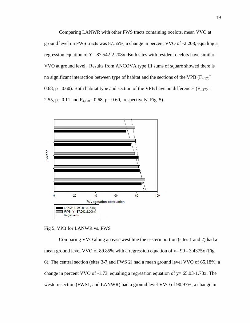
Comparing LANWR with other FWS tracts containing ocelots, mean VVO at

ground level on FWS tracts was 87.55%, a change in percent VVO of -2.208, equaling a

regression equation of Y= 87.542-2.208x. Both sites with resident ocelots have similar

VVO at ground level. Results from ANCOVA type III sums of square showed there is

no significant interaction between type of habitat and the sections of the VPB (F4,170=

0.68, p= 0.60). Both habitat type and section of the VPB have no differences (F1,170=

2.55, p= 0.11 and F4,170= 0.68, p= 0.60, respectively; Fig. 5).

Fig 5. VPB for LANWR vs. FWS

Comparing VVO along an east-west line the eastern portion (sites 1 and 2) had a

mean ground level VVO of 89.85% with a regression equation of y= 90 - 3.4375x (Fig.

6). The central section (sites 3-7 and FWS 2) had a mean ground level VVO of 65.18%, a

change in percent VVO of -1.73, equaling a regression equation of y= 65.03-1.73x. The

western section (FWS1, and LANWR) had a ground level VVO of 90.97%, a change in

20

percent VVO of -3.69, equaling a regression equation of y= 90.9722-3.69x, which was

similar to the eastern section.

Fig. 6. VPB comparing sites east-west

Results from ANCOVA type III sums of squares showed there is no significant

interaction between type of habitat and the sections of the VPB (F8,327=0.46, p= 0.87 ).

Vegetation Profile Board data differed between habitats found in the eastern, central, and

western sections of the potential habitat as indicated by the canopy cover map. Both

habitat type and section of the VPB are significantly different between habitat types

(F2,327=5.81, p =.003, and F4,327=3.61, p =.006 respectively).

Principal component (PC) axes I and II explained 55% of the variation in habitat

among all sites (Fig. 7). Strongest negative loadings for PC I were number of individuals

(-0.46), number of species (-0.40), diversity (-0.37) and intercept (-0.38). The strongest

positive loadings for PC I was woody plant height (0.35). The strongest negative loadings

21

17

for PC II was represented by percent bare ground (-0.43). Strongest positive loadings for

PC II were percent litter (0.50) and canopy cover (0.44).

Fig. 7. PCA biplot for all transects

The majority of the habitat at LANWR was characterized by increased plant density and

diversity, more vertical screening cover at ground level, more canopy cover, smaller

shrubs and more litter on the ground. A few outliers had more grass, more bare ground

and lower species abundance. The majority of FWS tracts fell into the same grouping as

LANWR, but with generally more canopy cover and more litter (Fig. 8).

22

Fig. 8. PCA for LANWR vs. FWS

Along the east-west line, habitats in the east were similar to LANWR with more

diversity, more canopy cover, smaller shrubs and more ground litter. The western habitats

(sites 1 and 2) were similar, except there were several transects that had more grass and

more bare ground. The middle group (sites 3-7 and FWS 2) were characterized by less

diversity, taller shrubs, more positive slopes, more grass, and more bare ground (Fig 9).

Fig. 9. PCA for sites east-west

23

17

Only one transect contained a positive VPB slope (more cover in shrubs at 2.0-2.5 meters

than at 0-0.5 meters). Habitat at site 1 followed the grouping of LANWR, also containing

a few outliers with more grass, bare ground, and lower abundance. Habitat at site 6 was

similar to LANWR, but was not as diverse. Habitats at sites 3 and 5 were less diverse,

with taller shrubs and a positive slope. Other habitats tended to fall in between the two

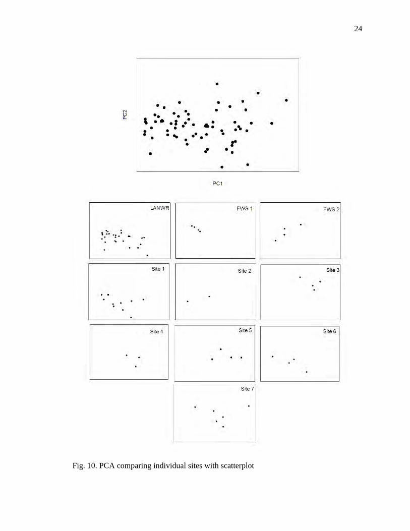
extremes of diversity (Fig. 10).

24

Fig. 10. PCA comparing individual sites with scatterplot

25

17

CHAPTER V

DISCUSSION

The majority of previous research on ocelot habitat and recovery plans has focused

on canopy cover. My research identifies additional components that might be important

in designating potential ocelot habitat. First, our analysis of C-CAP data showed that

ocelots preferred shrub/scrub, palustrine shrub/scrub, and grassland. Previous research

has shown that four of 11 ocelot dens were located in alkali sacaton grass, Sporobolus

airoides, and the den chamber consisted of grass bases (Laack et al. 2005). Therefore,

habitat with some grasses interspersed throughout dense shrub cover could be beneficial

for reproductive considerations. The C-CAP defines the palustrine shrub/scrub category

as a tidal and non-tidal wetland dominated by shrubs. My research showed that ocelots

selected for palustrine shrub/scrub, but we chose to remove it from the cover map

because it produced too coarse of a scale. Future research should look into possible

relationships of ocelots and these habitats, especially since prey are likely to be near

water and vegetation near water is more dense. My research showed that transects located

near intermittent water drainages were generally more dense. These areas are easily

found on any satellite image (i.e. Google Earth, Texas Natural Resources Information

System) and could be considered as ocelot travel corridors between habitats.

Plant species richness and density were components of ocelot habitat shown to be

important. Transects containing lower richness and density of plants generally were

26

dominated by honey mesquite shrubs with a high percentage of grass and tended to be in

areas grazed by cattle. Another instance where lower richness and abundance occurred

was on a FWS tract, next to La Sal Vieja, a large salt lake. The border around the salt

lake contained Willamar soil, a fine sandy loam. Willamar is moderately to strongly

alkaline at all horizons according to NRCS, which could prevent certain shrubs from

growing.

Soil analysis was identical to Harveson et al. (2004), but I decided to identify the

soil composition for each series to determine a key factor in soil use. While most of the

preferred soils were silty clay loams, half of the avoided soils were of a similar loam

type. All soils contained a substantial amount of clay. Box (1961) looked at relationships

between soil and similar plants (lotebush, blackbrush, brasil), and determined that no

significant differences existed between clay content in the soil samples of different plant

communities. I considered focusing on soil orders for this study but according to NRCS,

soil orders in South Texas are broken up from east to west, from Vertisols, Mollisols, and

Inceptisols. Vertisols generally have more clay that tends to shrink and swell with

moisture content. Mollisols are enriched with organic matter and are naturally fertile.

More to the west are Inceptisols which have weakly developed subsurface horizons. In

the northern counties are Alfisols, which contain more clay and 35% base saturation.

The region for Mollisols lined up with sites 3-7, which were least similar to ocelot habitat

based on the PCA results. Box (1961) also determined that there was a strong negative

correlation between potassium and shrub cover, suggesting that these shrubs grow best in

soils with low potassium. Consideration of chemical content in soil would likely be more

beneficial than focusing on soil texture/type or soil orders.

27

27

17

Vegetation profile board results were beneficial in determining the vertical structure

of vegetation cover. When identifying potential ocelot habitat, it is best to follow a

regression of Y= 90 - 3.929x for vertical structure. Transects that had a similar regression

were found to be similar to ocelot habitat in PCA analysis. Similar transects had a higher

intercept representing more VVO at ground level, and a more negative slope representing

greater change in VVO from ground level to 2.5 meters. The transects in the middle

section (sites 3-7 and FWS 2) of the map were least similar to ocelot habitat and had a

VVO at ground level of 65.18%. The minimum VVO at ground level on ocelot habitat

was 88%, which proved to be important on PCA, suggesting that dense cover at ground

level should be accounted for when searching for potential ocelot habitat, not just canopy

cover as stated in previous literature (Shindle and Tewes 1998, Harveson et al. 2004).

Overall, potential ocelot habitat is characterized by greater plant diversity, more

dense shrubs at ground level, more canopy cover, smaller shrubs and more litter on the

ground.

28

CHAPTER VI

MANAGEMENT IMPLICATIONS

Based on my results, potential habitat could be initially found using the brush map

produced by Sternberg (FWS, 2009), which delineates 75% canopy cover (Fig 11). Our

brush map uses shrub/scrub that C-CAP defines >20% of the total vegetative cover, so a

more specific map would be beneficial. Once potential habitat is identified, field

measurements need to be conducted on a wide array of vegetative parameters. Results

from future field research can be compared with our data to determine if habitat falls into

the same range on the PCA scatterplot. Additional parameters such as soil chemistry

might also be included in the analysis because of its influence on plant growth.

29

29

17

Fig. 11. Shrub/scrub cover map for South Texas produced by Sternberg (FWS, 2009)

The clearing of Tamaulipan brushland has eliminated more than 95% of all

brushland habitat. This habitat loss because of agriculture in addition to urbanization and

economic development has altered the area along the Texas-Mexico border (Chapman et

al. 1998). In order to compensate for this, agricultural lands need to be converted to

conservation lands to provide contiguous habitat for ocelots. Ocelots play a large role in

conserving the native habitat, primarily because they are considered a flagship species.

Conservation of land for ocelots also conserves land for other species in South Texas

such as the burrowing owl (Athene cunicularia), desert tortoise (Gopherus agassizii),

whitetail deer (Odocoileus virginianus), and white-wing dove (Zenaida asiatica).

Conserving land has proven effective to restoring species. After conservation land was

30

designated for the grizzly bear (Ursus arctos), the species recolonized back from 2% to

almost 50% of its original habitat (Pyare, 2004). A landscape with carnivores, implying

intact food web, has high potential for ecological integrity (Noss et al. 1996). It is

important when designating conservation land to consider the habitat requirements of

carnivore species to improve the umbrella function (Noss et al. 1996). To do so, we

should turn to private landowners who own large tracts of potential ocelot habitat (Haines

et al. 2005). Programs such as the Conservation Reserve Program (CRP) offered through

the Farm Bill and the Landowner Reserve Program (LRP) offered by Texas Parks and

Wildlife provide private landowners incentive to conserve land. At least half of the sites I

studied would not provide suitable habitat for ocelots today. Conservation incentives

could be used to restore native shrubland by using brush control to encourage basal

sprouting, and by planting adapted native shrubs (Campbell and Armstrong 1997).

Managers interested in restoring their land can construct shelters to enhance seedling

growth and establishment (Young and Tewes 1994).

Evaluation of release sites will begin in 2010 and translocation shall begin in

2011 (Translocation Team 2009). It is now known that ocelots require more than just

canopy cover for ideal habitat and other vegetative components (i.e. VVO and plant

diversity) can be analyzed to identify potential habitat. Ocelot habitat can now be defined

as requiring >75% canopy cover, a mean plant density of >20 individuals/100 m2, high

plant diversity (<0.20 D), <15% grasses, >50% litter, and a VVO regression of Y= 90 -

3.929x. The most important components to identify in the field would be number of

woody plant individuals and number of woody species, percent bare ground, percent litter

and canopy cover. Importance of plant diversity and density could be a correlation with

31

31

17

prey (rodents, birds, etc.) availability/density. Future research should identify prey

availability on potential habitat. Generally areas with high number of mesquite trees had

less overall plant diversity, density, and more grass. It’s possible that areas with high

mesquite can immediately be ruled out of the potential habitat selection process.

Furthermore areas along the Rio Grande (the Lower Rio Grande Valley) are subjected to

high urbanization with high road density (fig.11). The USFWS Translocation Plan

recommends to avoid roads with high-speed and/or high-volume traffic. Therefore I

recommend biologists to search for potential habitat along the northern border of Willacy

and Starr counties and further north and to avoid the northern border of Hidalgo county

which is inundated with a geological sand sheet, creating less ideal habitat, as stated in

the “middle” section of my study area. Areas containing intermittent water drainages may

be used as corridors between habitats. Incentive programs offered by local and national

governments may be used to build corridors and/or restore native shrubland. With the

cooperation of the government, biologists, and private landowners, there is a chance to

recover ocelots.

32

APPENDIX

C-CAP descriptions of land-use/land-cover classes

Land classification C-CAP description

high intensity developed Includes highly developed areas where people reside

or work in high numbers. Impervious surfaces

account for 80 to 100 percent of the total cover.

medium intensity developed Includes areas with a mixture of constructed

materials and vegetation. Impervious surfaces

account for 50 to 79 percent of the total cover.

low intensity developed Includes areas with a mixture of constructed

materials and vegetation. Impervious surfaces

account for 21 to 49 percent of total cover.

developed open space Includes areas with a mixture of some constructed

materials, but mostly vegetation in the form of lawn

grasses. Impervious surfaces account for less than 20

percent of total cover.

cultivated Areas used for the production of annual crops. Crop

vegetation accounts for greater than 20 percent of

total vegetation. This class also includes all land

being actively tilled.

pasture/hay Areas of grasses, legumes, or grass-legume mixtures

planted for livestock grazing or the production of

seed or hay crops, typically on a perennial cycle and

not tilled.

grassland Areas dominated by grammanoid or herbaceous

vegetation, generally greater than 80 percent of total

vegetation. These areas are not subject to intensive

management such as tilling, but can be utilized for

grazing.

deciduous forest Areas dominated by trees generally greater than 5

meters tall and greater than 20 percent of total

vegetation cover. More than 75 percent of the tree

species shed foliage simultaneously in response to

seasonal change.

evergreen forest Areas dominated by trees generally greater than 5

meters tall and greater than 20 percent of total

vegetation cover. More than 75 percent of the tree

species maintain their leaves all year. Canopy is

never without green foliage.

33

33

17

mixed forest Areas dominated by trees generally greater than 5

meters tall, and greater than 20 percent of total

vegetation cover. Neither deciduous nor evergreen

species are greater than 75 percent of total tree cover.

shrub/scrub Areas dominated by shrubs less than 5 meters tall

with shrub canopy typically greater than 20 percent

of total vegetation.

palustrine forested wetland Includes all tidal and nontidal wetlands dominated

by woody vegetation greater than or equal to 5

meters in height, and all such wetlands that occur in

tidal areas in which salinity due to ocean-derived

salts is below 0.5 percent. Total vegetation coverage

is greater than 20 percent.

palustrine scrub/shrub wetland Includes all tidal and non tidal wetlands dominated

by woody vegetation less than 5 meters in height, and

all such wetlands that occur in tidal areas in which

salinity due to ocean-derived salts is below 0.5

percent. Total vegetation coverage is greater than 20

percent.

palustrine emergent wetland Includes all tidal and nontidal wetlands dominated

by persistent emergent vascular plants, emergent

mosses or lichens, and all such wetlands that occur in

tidal areas in which salinity due to ocean-derived

salts is below 0.5 percent. Plants generally remain

standing until the next growing season. Total

vegetation cover is greater than 80 percent.

estuarine forested wetland Includes all tidal wetlands dominated by woody

vegetation greater than or equal to 5 meters in height,

and all such wetlands that occur in tidal areas in

which salinity due to ocean-derived salts is equal to

or greater than 0.5 percent. Total vegetation coverage

is greater than 20 percent.

estuarine scrub/shrub wetland Includes all tidal wetlands dominated by woody

vegetation less than 5 meters in height, and all such

wetlands that occur in tidal areas in which salinity

due to ocean-derived salts is equal to or greater than

0.5 percent. Total vegetation coverage is greater than

20 percent.

34

unconsolidated shore Unconsolidated material such as silt, sand, or gravel

that is subject to inundation and redistribution due to

the action of water. Characterized by substrates

lacking vegetation except for pioneering plants that

become established during brief periods when

growing conditions are favorable. Erosion and

deposition by waves and currents produce a number

of landforms representing this class.

bare land Generally, vegetation accounts for less than 10

percent of total cover.

water All areas of open water, generally with less than 25

percent cover of vegetation or soil.

35

LITERATURE CITED

Anderson, J.R., E.E. Hardy, J.T. Roach, and R.E. Witmar. 1976. A land use and land

cover classification system for use with remote sensor data. U.S. Geological

Survey Professional Paper 964, U.S. Government Printing Office, Washington,

D.C.

Beyer, H.L. 2004. Hawth's Analysis Tools for ArcGIS. Available at

http://www.spatialecology.com/htools.

Bezanson, D. 2001. The South Texas Plains and Lower Rio Grande Valley in: Natural

vegetation types of Texas and their representation in Conservation Areas. 79-98.

Broad, S. 1987. International trade in skins of Latin American spotted cats. Traffic

Bulletin 9: 56-63.

Bryant, D.M., M.J. Ducey, J.C. Innes, T.D. Lee, R.T. Eckert and D.J. Zarin. 2004. Forest

community analysis and the point-centered quarter method. Plant Ecology.

175(2): 193-203.

Box, T.W. 1961. Relationships between plants and soils of four range plant communities

in South Texas. Ecology 42(4): 794-810.

Campbell, L. and A. Armstrong. 1997. Managing brush and maintaining habitat for

endangered species. Texas Natural Resource Server Symposia.

Carroll, C. Noss, R.F., and Paquet, P.C. 2001. Carnivores as focal species for

conservation planning in the Rocky Mountain region. Ecological Applications

11(4): 961-980.

Chapman, D.C., D.M. Papoulias, and C.P. Onuf. 1998. Environmental Change in South

Texas. pp 43-46 in M.J. Mac, P.A. Opler, and P.D. Doran, eds. Status and Trends

of the Nation's Living Resources. U.S. Department of the Interior, USGS

Biological Resources Division. Washington, D.C. 964 pp.

Haines, A.M., M.E. Tewes, L.L. Laack, W.E. Grant and J.H. Young. 2005.

Evaluating recovery strategies for an ocelot (Leopardus pardalis) population in

the united states. Biological Conservation 126: 512-522.

36

Haines, A.M., M.E. Tewes, L.L. Laack, J.S. Horne and J.H. Young. 2006a. A

habitat-based population viability for ocelots (L. pardalis) in the U.S. Biological

Conservation 132: 424-436.

Haines, A.M., L.I. Grassman Jr., M.E. Tewes and J.E. Janecka. 2006b. First ocelot

(Leopardus pardalis) monitored with GPS telemetry. European Journal of

Wildlife Research 52: 216-218.

Harveson, P.M., M.E. Tewes, G.l. Anderson and L.L. Laack. 2004. Habitat use by

ocelots in south Texas: implications for restoration. Wildlife Society Bulletin

32(3): 948-954.

Horne, J.S., A.M. Haines, M.E. Tewes, and L.L. Laack. 2009. Habitat partitioning by

sympatric ocelots and bobcats: implications for recovery of ocelots in southern

Texas. The Southwestern Naturalist 54(2): 119-126.

Jackson, V.L., Laack, L.L. and E.G. Zimmerman. 2005. Landscape metrics

associated with habitat use by ocelots in south Texas. Journal of Wildlife

Management 69(2): 733-738.

Laack, L.L, M.E. Tewes, A.M. Haines and J.H. Rappole. 2005. Reproductive life history

of ocelots (Leopardus pardalis) in southern Texas. Acta Theriologica 50(4): 505-

514.

Murray, Julie L. and G.L. Gardner. 1997. Leopardus pardalis. Mammalian Species 548:

1-10.

Nudds, T.D. 1977. Quantifying the vegetative structure of wildlife cover. Wildlife

Society Bulletin 5(3): 113-117.

R Development Core Team. 2005. R: A language and environment for statistical

computing. R Foundation for Statistical Computing, Vienna, Austria.

ISBN 3-900051-07-0, URL http://www.R-project.org.

Schmidly, D.J. 1977. The mammals of Trans-Pecos Texas. Texas A&M University Press,

College Station. 225 pp.

Shindle, D.B. and M.E. Tewes. 1998. Woody species composition of habitats used

by ocelots (Leopardus pardalis) in the Tamaulipan Biotic Province.

Southwestern Naturalist 43(2): 273-278.

Translocation Team (A Subcommittee of the Ocelot Recovery Team). 2009. Plan for

Translocation of Northern Ocelots (Leopardus pardalis albescens) in Texas and

Tamaulipas.

37

17

Trolle, Mogens and K. Marc. 2003. Estimation of ocelot density in the Pantanal using

capture-recapture analysis of camera-trapping data. Journal of Mammalogy

84(2): 607-614.

U.S. Fish and Wildlife Service. 2006. Draft Ocelot (Leopoldus pardalis) Recovery Plan

(revised). U.S. Fish and Wildlife Service, Southwest Region, Albuquerque, NM.

Young, J.H. and M.E. Tewes. 1994 Evaluation of techniques for initial restoration of

ocelot habitat. Proceedings of the Annual Conference of the Southeastern

Association of Fish and Wildlife Agencies. 48: 336-342.

VITA

Amy R. Connolly was born in Santa Fe, N.M. to Susan DeLong and R. Perry

Connolly in 1978. She came to Texas as quick as she could and aspired to be involved

with the welfare of animals. She worked as the head animal caretaker at a local animal

sanctuary while she attended Texas State University-San Marcos. She graduated with a

B.S. in Biology in 2002. During her undergraduate studies, she was inspired by Dr.

Simpson to pursue a career in wildlife research. This inspiration made her enter the M.S.

Wildlife Ecology program in 2007, with Dr. Simpson as her advisor. She immersed

herself in multiple research projects and served as secretary for the Student Chapter of

The Wildlife Society. Amy's passion for wildlife and the outdoors serves as the

motivation for her life's work and she is grateful for the never-ending support from her

friends and family.

Permanent Address: 3310 Robinson Avenue

Austin, Texas 78722

This thesis was typed by Amy Rosamond Connolly.

17