defining unemployment in developing countries: the case … · credit research paper no. 01/09...
TRANSCRIPT

_____________________________________________________________________CREDIT Research Paper
No. 01/09_____________________________________________________________________
Defining Unemployment in DevelopingCountries: The Case of Trinidad and
Tobago
by
David Byrne and Eric Strobl
_____________________________________________________________________
Centre for Research in Economic Development and International Trade,University of Nottingham

The Centre for Research in Economic Development and International Trade is basedin the School of Economics at the University of Nottingham. It aims to promoteresearch in all aspects of economic development and international trade on both along term and a short term basis. To this end, CREDIT organises seminar series onDevelopment Economics, acts as a point for collaborative research with other UK andoverseas institutions and publishes research papers on topics central to its interests. Alist of CREDIT Research Papers is given on the final page of this publication.
Authors who wish to submit a paper for publication should send their manuscript tothe Editor of the CREDIT Research Papers, Professor M F Bleaney, at:
Centre for Research in Economic Development and International Trade,School of Economics,University of Nottingham,University Park,Nottingham, NG7 2RD,UNITED KINGDOM
Telephone (0115) 951 5620Fax: (0115) 951 4159
CREDIT Research Papers are distributed free of charge to members of the Centre.Enquiries concerning copies of individual Research Papers or CREDIT membershipshould be addressed to the CREDIT Secretary at the above address. Papers may alsobe downloaded from the School of Economics web site at: www.nottingham.ac.uk/economics/research/credit

_____________________________________________________________________CREDIT Research Paper
No. 01/09
Defining Unemployment in DevelopingCountries: The Case of Trinidad and
Tobago
by
David Byrne and Eric Strobl
_____________________________________________________________________
Centre for Research in Economic Development and International Trade,University of Nottingham

The AuthorsDavid Byrne is Associate Professor, Department of Economics, University ofVirginia, and Eric Strobl is Lecturer, Department of Economics, University College,Dublin.
AcknowledgementsThanks are due to Peter Pariaj and the Trinidad and Tobago CSO for assistance withand provision of data. We are also grateful to Kevin Denny, Holger Goerg, and FrankWalsh for comments on an earlier draft and to Ralph Hussmanns and ConstanceSorrentino for advice on various aspects. All remaining errors are, of course, ourown.
____________________________________________________________ May 2001

Defining Unemployment in Developing Countries: The Case of Trinidad andTobago
byDavid Byrne and Eric Strobl
AbstractThe International Labour Organisation (ILO) argues for relaxing the standard definitionof unemployment in developing countries where labour markets are not as efficient asthose in the developed world. We examine whether such an extension of the standarddefinition is appropriate in the case of Trinidad and Tobago. Specifically, we useindividual behaviour to classify persons into labour market states, rather than a prioricriteria like job search. The Trinidad and Tobago Continuous Survey Sample ofPopulation provides data uniquely suited to this purpose. Our results indicate that inTrinidad and Tobago males, who under the standard criteria would be considered out ofthe labour force because they report willingness to work but are not currently searchingfor a job, are appropriately classified as unemployed. Further evidence suggests that thismay be because job search may not be as meaningful in rural as it is in urban areas.
Outline1. Introduction2. ILO Definition of Unemployment3. T&T Definition of Unemployment4. Empirical Framework5. Unconditional Transition Probabilities6. Econometric Analysis7. Conclusion


1
I. INTRODUCTION
The unemployment rate is the most widely used indicator of the well-being of a labour
market and an important measure of the state of an economy in general. While the
unemployment rate is in theory straightforward, classifying working age persons as either
employed, unemployed, or out of the labour force is difficult in practice. To facilitate
comparisons of unemployment rates over time and across countries, the International
Labour Organisation (ILO) has since 1954 set forth guidelines for categorising
individuals into these labour market states.1 These have now been adopted, at least
in some form, by most developed and a large number of developing countries, which has
allowed the ILO to compile a sizeable number of roughly comparable labour market
statistical series across countries and over time.
According to the ILO guidelines, a person is unemployed if the person is (a) not working,
(b) currently available for work and (c) seeking work. Practical implementation of these
guidelines is, however, generally difficult. While employed persons are relatively easily
classified in most countries, the issue of classifying non-employed persons as either
unemployed or out of the labour force, especially according to criteria (c) is not
uncontroversial; see, for instance, OECD (1987, 1995). For instance, the requirement of
job search is attractive because it requires active demonstration of attachment to the
labour force, but it also classifies a large number of non-searchers as out of the labour
force. Some economists would argue that availability and willingness to work are
sufficient to distinguish workers in the labour force from the non-attached. Moreover,
while the requirement of active job search may be meaningful in industrialised countries
where the bulk of the population engages in paid employment and where there are clear
channels for the exchange of labour market information. This may not be the case in
many developing countries where search may be more costly and job search behavior is
less meaningful, especially in large rural sectors.2
In view of this in 1982 the ILO Thirteenth International Conference of Labour
Statisticians revised its definition of unemployment in the sense of introducing certain
1 See the proceedings of the Eight International Convention of Labour Statisticians (1954).
2 See Hussmanns (1994).

2
amplifications concerning, amongst other things, the criteria of seeking work and the
statistical treatment of people currently available for work but not actively seeking work.
These amplifications, allowing for more broader definitions of unemployment, were
specifically “aimed to make it possible to measure unemployment more accurately and
more meaningfully both in developed and developing countries alike” (ILO, 1998, p. 52).
Ultimately the question of how to best define unemployment boils down to which
categories of non-employed people should be considered part of the labour force. The
most obvious way to determine this is to take sub-groups of the non-employed, say those
not searching but willing to work, and compare their transition probabilities into
employment and/or some other labour market state to those of a benchmark group, for
example the searching non-employed. This approach is, of course, not new to the
economics literature, although the evidence has been mixed and almost exclusively
focused on the US and Canada; see, for instance, Hall (1970), Clark and Summers
(1979), Clark and Summers (1982), Flinn and Heckman (1983), Gonül (1992) and, more
recently, Jones and Riddell (1999).
Although job search as a prerequisite for being considered unemployed may arguably not
be appropriate in developing countries, a similar line of research in a developing country
context has, except for Kingdon and Knight (2000), however, remained unexplored.
Limited to only cross-sectional data on the unemployed in South Africa, Kingdon and
Knight (2000) are not able to directly test whether unemployed searchers and non-
searchers in a developing country are behaviourally distinct in terms of their labour
market state transitions, but instead explore the determinants of job search among the
non-employed and estimate local wage-unemployment relationships. The authors find
that the non-searching are more deprived than the searching unemployed and that many
unemployed do not search because they are discouraged, suggesting that financial
constraints rather than tastes cause the non-employed not to search. Moreover, they
present evidence showing that local wage determination takes non-searchers into account
as genuine labour force participants. Both of these factors are taken as evidence in
support of adopting a definition of unemployment in South Africa that includes the non-
searching non-employed.

3
In this paper we address the problem of defining unemployment in a developing country
context by studying the definition of unemployment employed in Trinidad and Tobago
(T&T). T&T serves as an ideal case study in that since the early 1960s it has used a
more flexible definition of unemployment than that prescribed by the original stringent
ILO criteria because it was felt that the latter was not appropriate for the underdeveloped
T&T labour market. Specifically, non-employed working age persons in T&T are
considered to be unemployed not only if they are currently actively seeking jobs, but also
if they are willing and able to work and are currently not seeking, but have looked for
work some time in the last three months prior to the interview - a group which we refer
to as the `marginally attached’.3 In T&T, as in other developing countries4, such
marginally attached are a non-negligible group - for instance, in 1998 their exclusion
from the unemployed would have lowered the official unemployment rates for males and
females by over three and five percentage points, respectively.
To investigate whether the marginally attached behave more like non-employed active
job seekers or those out of the labour force, we employ the methodology of Jones and
Riddell (1999). Accordingly, we follow persons categorised in these groups over time
to see whether their transition rates to other labour market states are similar in magnitude
and in the effect of covariates on the transitions. The groups which are behaviourally
similar in outcome could arguably be grouped together into the same labor force state.
For this task we have access to three years of the T&T Continuous Sample Survey of
Population data which allows us to construct a panel of individuals’ labour market state
transitions over time.
The paper is organised as follows. In Section II we outline and discuss more extensively
the ILO definition of unemployment and its application to labour markets of developing
countries. Section III provides a description and analysis of the definition of
unemployment utilised in T&T. The subsequent section outlines the framework
developed by Jones and Ridder (1999) used to determine behavioural equivalence among
labour market states. Our analysis, using this framework, of the unconditional transition
3 The term ‘marginally attached’ is also used by the ILO and by Jones and Riddell (1999), although in both cases
its use is somewhat different from here.
4 Kingdon and Knight (2000) find for South Africa that including all non-searchers that are willing to work
increases the total unemployment rate by 15 percentage points in 1997.

4
probabilities across labour market states of males and females in T&T using three years
of panel data from the T&T Continuous Sample Survey of Population is contained in
Section IV. An econometric investigation of the conditional transition probabilities is
found in Section V. Finally, concluding remarks are given in the last section.
II ILO DEFINITION OF UNEMPLOYMENT
Although the earliest efforts to establish international statistical standards of the
measurement of unemployment can be traced back to 1895, the definition of
unemployment currently recommended by the ILO has its roots in a resolution by the
Eighth International Conference of Labour Statisticians (ICLS), convened by the ILO in
Geneva in 1954. The ILO approach to defining unemployment rests on what can be
termed the ‘labour force framework’, which at any point in time classifies the working
age population into three mutually exclusive and exhaustive categories according to a
specific set of rules: employed, unemployed, and out of the labour force - where the
former two categories constitute the labour force, i.e., essentially a measure of the supply
of labour at any given time.5
Although the definition of unemployment has since 1954 been periodically revised its
basic criteria remains intact. Accordingly, a person is to be considered unemployed if
he/she during the reference period simultaneously satisfies being:
(a) ‘without work’, i.e., were not in paid employment or self-employment as
specified by the international definition
(b) ‘currently available for work’, i.e., were available for paid employment or
self-employment during the reference period; and
(c) ‘seeking work’, i.e., had taken specific steps in a specified recent period to
seek paid employment or self-employment.
The ‘without work’ condition serves to distinguish between the employed and the
unemployed, and thus guarantees that these are mutually exclusive categories of the
5 This set of rules is characterised by three features: (a) a reference period, (b) an activity status which allows the
categorisation of the working age population into the aforementioned three categories on the basis of
activities performed during the reference period, and (c) a set of priority regulations to ensure that persons
can only be classified into one of these three categories.
5
working age population, whereas the latter two criteria separate the non-employed into
the unemployed and the out of labour force. The purpose of the availability for work
condition is to exclude those individuals who are seeking work to start at a later date, and
thus is a test of current readiness. The intention of the seeking work criterion is, on the
other hand, to ensure that a person will have taken certain ‘active’ steps to be classified
as unemployed.
The ILO itself notes that its labour force framework used to define unemployment is best
suited to “situations where the dominant type of employment is regular full-time paid
employment...(and that in) practice, however, the employment situation in a given
country...will to a greater or lesser degree differ from this pattern” (ILO, 1994).
Moreover, the Thirteenth ICLS resolution provided a number of amplifications with
regard to the measurement of unemployment that were specifically, as noted earlier,
aimed to make it possible to measure unemployment more accurately and more
meaningfully both in developed and developing countries alike. The one that is of
particular interest here is the provision to allow for a relaxation of the search criteria
which states that in “situations where the conventional means of seeking work are of
limited scope, where labour absorption is, at the time, inadequate, or where the labour
force is largely self-employed, the standard definition of unemployment...may be applied
by relaxing the criterion of seeking work” (ILO, 1983, p. xi). In particular, Hussmanns
et al (1990) note that “seeking work is essentially a process of search for information on
the labour market...(and) in this sense, it is particularly meaningful as a defining criterion
in situations where the bulk of the working population is oriented towards paid
employment and where channels for the exchange of labour market information exist and
are widely used.....this may not be the case in developing countries” (p. 105).6

6
Table 1: Reference Period and Unemployment Job Search Period for Developedand Developing Countries
DEVELOPED COUNTRIESAustralia (1 week - 4 weeks), Austria (1 week - 4 weeks), Bahamas (1 week - 4 weeks),Belgium (1 week - 4 weeks), Caiman Islands (1 week - 1 week), Canada (1 week - 4weeks), Cyprus (1 week - 1 month), Denmark (1 week - 4 weeks), Finland (1 week - 4weeks), France (1 week - 1 month), Germany (1 week - 4 weeks), Greece (1 week - 4weeks), Guam (1 week - 4 weeks), Hong Kong (1 week - 1 month), Ireland (1 week - 1week), Israel (1 week - 1 week), Italy (1 week - 4 weeks), Japan (1 week - 1 week),Luxembourg (1 week - 1 week), Netherlands (1 week - 4 weeks), Netherlands Antilles(1 week - 4 weeks), New Zealand (1 week - 4 weeks), Norway (1 week - 4 weeks),Portugal (1 week - 1 month), Singapore (1 week - 4 weeks), Slovenia (1 week - 1 week),Spain (1 week - 4 weeks), Sweden (1 week - 4 weeks), United Kingdom (1 week - 4weeks), United States (1 week - 4 weeks);
DEVELOPING COUNTRIESArmenia (1 week - 1 week), Barbados (1 week - 4 weeks), Bolivia (1 week - 1 week),Botswana (1 week - 1 week), Brazil (1 week - 1 week), Bulgaria (1 week - 1 month),Chile (1 week - 2 months), Columbia (1 week - 1 week), Costa Rica (1 week - 5 weeks),Cuba (1 week - 4 weeks), Czech Republic (1 week - 1 week), Ecuador (1 week - 5weeks), Egypt (1 week - 1 week), Estonia (2.5 years - 1 week), Ethopia (1 week - Non-Searchers included), French Guiana (1 week - 1 month), Guadoloupe (1 week - 1month), Guatemala (1 week - 5 weeks), Honduras (1 week - 5 weeks), Hungary (1week - 1 month), India (1 week - 1 week), Indionesia (1 week - 1 week), Jamaica (1week - Non-Searchers included), Kenya (1 day - 1 week), Korea (1 week - 1 week),Latvia (1 week - 1 month), Lithuania (1 week - 1 week), Macedonia (1 week - 1 week),Malawi (1 week - Non-Searchers included), Malaysia (1 week - 3 months), Martinique(1 week - 1 month), Maritius (1 week - 8 weeks), Nigeria (1 week - 1 week), Pakistan (1week - Non-Searchers included), Panama (1 week - Non-Searchers included),Paraguay (1 week - 1 week), Peru (1 week - Non-Searchers included), Philippines (1week - Non-Searchers included), Poland (1 week - 1 week), Puerto Rico (1 week - 1week), Romania (1 week - 1 week), Russian Federation (1 week – 1 week), Slovakia (1week - 1 month), Slovenia (1 week - 1 week), South Africa (1 week - 4 weeks), SriLanka (1 week - Non-Searchers included), Syrian Arab Republic (1 week - 1 week),Thailand (1 week - Non-Searchers included), Trinidad and Tobago (1 week - 3months), Tunisia (1 week - Non-Searchers included), Turkey (1 week - 6 months),Ukraine (1 week - 1 week), Uruguay (1 week - 1 week), Venezuela (1 week - Non-Searchers included);
Notes:1. Source: ILO (1990) and various issues of the Bulletin of Labour Statistics (ILO).2. The first period in the parentheses is the reference period, while the second is the unemployment job search
period required for inclusion among the unemployed.
6 For instance, in T&T there is neither an unemployment compensation system nor any well developed
employment exchange system. Such features clearly make the job search process different to that found in
developed countries.

7
The relaxation of the search criteria may entail a full relaxation or a partial one in the
sense of including, “in addition to persons satisfying the standard definition, certain
groups of persons without work who are currently available for work but who are not
seeking work for particular reasons” (Hussmanns et al, 1990, p. 106). One way to ensure
that persons, who are not currently seeking work but are willing and able to work, have
at least in the past demonstrated some attachment to the labour force is to, as in the case
of Trinidad and Tobago, require these to have sought work in some prior specified
period. In Table 1 we have compiled information on the reference period and the period
of job search of the household surveys of various countries used to define the
unemployed. As can be seen from the countries listed in this table, many countries, both
developing and developed, do indeed extend their job search beyond the reference period
of their household survey. For those developed countries that do use a longer job search
period than the reference period, the period used for job search does not exceed one
month. This lies in contrast to a number of developing countries whose job search
period reaches up to 12 months, and/or whose unemployed include also all those that do
not search at all but are willing and able to work.
III T&T DEFINITION OF UNEMPLOYMENT
The Central Statistics Office (CSO) in T&T has been carrying out a labour force survey,
known as the Continuous Sample Survey of Population (CSSP), since 1963 and which
has served as T&T’s primary source of providing up-to-date data on the labour force
characteristics of residents of T&T, particular the incidence of unemployment.7 As
noted earlier, the definition of unemployment adopted in T&T is broader than that
employed in almost all developed countries and some developing countries.
Specifically, the CSO defines the unemployed as not only those non-employed that are
currently job seekers, but also includes those non-active job seekers that looked for work
7 The CSSP is a household survey based on a stratified clustering design, and, while originally conducted semi-
annually, has since 1987 been carried out on a quarterly basis.

8
during the three month period preceding the interview and who at the time of interview
did not have a job but still wanted work.8, 9
This expanded definition of unemployment was recommended by a committee set up to
advise the CSO “on the labour force concepts and definitions most meaningful for
Trinidad and Tobago” (CSO, p. 180) prior to the commencement of the CSSP in 1963.
In particular it was “...felt that in a developing country where jobs are scarce and where
there is not a well recognised system of unemployment registration, a week is too short
of a reference period as regards ‘looking for work’, while reliance on respondents
volunteering information that they wanted to work although they did not seek work
might result in loss of some persons who should be included” (CSO, p. 180). One
should thus note that this definition and its justification substantially precede the official
modifications of the more stringent ILO definition by the ILO itself in 1982.
Using the aggregate results on the T&T labour force derived from the CSSP and
published by the CSO we were able to calculate the male and female unemployment
rates since the start of the survey. Fortunately, the CSO has continuously disaggregated
the unemployed into the active job seekers and marginally attached, which then allows us
to derive a series of the unemployment rate also under the more stringent ILO
definition.10 The unemployment rates for males and females are given in Figures 1 and
2, respectively.
For males the unemployment rate in T&T, which is a petroleum based economy, had
risen from around 11 per cent in the early 1960s to 15 per cent by the early 1970s, until
the two oil shocks during that decade caused its fall to as low as eight per cent in 1980.
The deep economic crisis in the mid-1980s, caused by the fall in oil prices as well as a
8 One should note that any type of job search is considered legitimate. For a discussion of the distinction of active
and passive job search see Sorrentino (2000).
9 Individuals are categorised as unwilling or unable to work, and hence as out of the labour force, if in response to
the question of why they did not search for a job during the reference week they answered that they were (a)
at school, (b) housekeeping, (c) retired, or (d) did not want to work. The reasons which are deemed to
demonstrate a person’s willingness and ability to work are (a) temporary illness, (b) awaiting results of
application, (c) knew of no vacancy, (d) discouraged, and (e) some other (than the choices provided) reason
for not seeking work.
10 The CSSP publication labels those here referred to as marginally attached as ‘other unemployed’ and those
unemployed under the ILO definition as ‘unemployed seeking work’.

9
depletion in oil reserves, took a deep toll on the T&T male labour market, however, and
the male rate of unemployment peaked at nearly 22 per cent of the labour force during
this time. Since then the unemployment rate has again, in part due to fairly radical
policy changes, been consistently falling and now stands at a slightly higher level than
that found in the 1960s.
Figure 1: Male Unemployment Rate 1963-97
0
0,05
0,1
0,15
0,2
0,25
1963
1965
1967
1969
1971
1973
1975
1977
1979
1981
1983
1985
1987
1989
1991
1993
1995
1997
year
unem
ploy
men
t rat
e
URATE-T&T
URATE-ILO
Difference
As is also shown, the male unemployment rate defined according to the more stringent
ILO criteria follows a virtually identical cyclical pattern as the one just described. Its
level is, however, considerably lower than that derived under the T&T definition, on
average about 3.6 percentage points. Moreover, a closer look reveals that the difference
between the two series is positively related to their levels. The probable explanation for
this positive correlation is, of course, intuitive – during bad times the probability of
finding a job is substantially lower and hence more non-employed persons are
discouraged from searching.
The overall trends of the female unemployment rate are, except for the 1970s, similar to
that of males. What is strikingly different, however, is the difference in the rate of
unemployment as defined by the ILO and the T&T criteria. On average, the T&T
definition is 7.2 percentage points higher and has ranged from between 4.1 and 10.3

10
percentage points. Moreover, simple examination of the series does not suggest any
correlation between their levels and difference.
Figure 2: Female Unemployment Rate 1963-97
0
0,05
0,1
0,15
0,2
0,25
0,3
1963
1965
1967
1969
1971
1973
1975
1977
1979
1981
1983
1985
1987
1989
1991
1993
1995
1997
year
unem
ploy
men
t rat
e
URATE-T&T
URATE-ILO
Difference
Clearly, the marginally attached are a sizeable number in the T&T labour force and their
inclusion significantly raises the unemployment rate for both males and females. In
order to gain some insight into how these may differ from the unemployed that are
actively seeking jobs, we estimated a simple probit model of the probability of being a
current non-searcher conditional on being classified as unemployed according to the
T&T criteria for the male and female samples separately.11 As explanatory variables we
included a person’s age (allowing for non-linearity), whether that person resided in an
urban area, their marital status, educational dummy variables for the person’s highest
education attainment in terms of either primary education, secondary education O levels,
secondary education A levels, or university education12, and whether any elderly, defined
as persons over the age of 65, or children below the age of 6 reside in the same
household.13 The latter two variables were included to account for the fact that in T&T,
11 We chose to use a binary probit rather than a binary logit model in order to be able to calculate marginal
effects. It should be noted, however, that for all specifications logit estimation gave us qualitatively and
quantitatively similar results for all explanatory variables.
12 The base category is thus education at a level lower than primary education.
13 All estimations also include year and seasonal dummies, although the results are not reported.

11
like in many developing countries, many households additionally house extended family
members.14 These may have an impact on a person’s choice of labour market status
given that the social security system in T&T is fairly undeveloped so that the extended
and immediate family often play an important role in providing for the elderly and
children of their own and those of other family members residing in the household.15
The results of the probit estimation, the coefficients of which are reported as marginal
effects, are given in Table 2.16
Table 2: Determinants of the Probability of being Marginally Attached Relative tothe Unemployed (Job Seeking) and those Out of the Labour Force - Probit
Estimates
Unemployed Out of the Labour Force
Male Female Male FemaleUrban -0.178***
(0.029)-0.251***
(0.028)-0.057***
(0.012)-0.034***
(0.008)Marital Status -0.019
(0.046)0.045
(0.037)-0.065***
(0.016)-0.109***
(0.008)Age -0.031***
(0.006)-0.041***
(0.007)0.049***(0.002)
0.013***(0.001)
Age2 4.38e-04***(8.13e-05)
5.39e-04***(1.02e-04)
-6.23e-04***(2.93e-05)
-1.75e-04***(1.40e-05)
Primary Ed. -0.071*(0.037)
-0.022(0.040)
-0.068***(0.018)
-0.010(0.010)
Sec. Ed. (O) -0.060(0.048)
-0.087**(0.044)
-0.072***(0.014)
-0.081***(0.016)
Sec. Ed. (A) 0.124(0.133)
0.053(0.105)
-0.097***(0.012)
0.043(0.037)
Univ. Ed. -0.295(0.144)
-0.028(0.125)
-0.117***(0.089)
-0.027(0.041)
Children 0.010(0.035)
0.004(0.031)
0.047***(0.019)
0.004(0.008)
Elderly 0.010(0.038)
0.082*(0.042)
0.065***(0.019)
0.009(0.011)
nobs. 1249 1333 2628 5518X2(11) 90.96*** 127.90*** 879.48*** 513.93***Ps. R2 0.05 0.07 0.31 0.121: ***, **, and * signify one, five, and ten per cent significance levels, respectively.2: Coefficients are reported as marginal effects.3: All regressions include year and seasonal dummies.4. Robust std. errors in parentheses.
14 Both are defined as zero-one type dummies.
15 For example, the average household in our data set consisted of seven members and the standard deviation of
its size was four.
16 For all estimations we only included non-disabled individuals older than 14 years.

12
Accordingly, in terms of personal and household characteristics the job seeking males do
not appear to be substantially different from those that are marginally attached. We find
that rural residents are 17.8 per cent more likely to be marginally attached than urban
residents. The younger unemployed are also more likely to be marginally attached,
although this effect occurs at a decreasing rate. However, in terms of educational levels
only primary education has a significant effect on the probability of being marginally
attached. Higher levels of education, marital status and the presence of elderly or small
children in the household, in contrast, cannot serve to accurately predict whether a male
unemployed is currently job seeking or not. For females, in contrast, the composition of
the household, at least in terms of whether elderly are present, is differently distributed
across the two categories of unemployed. Those with elderly persons living in their
household are more likely to be marginally attached. Differences in individual
characteristics are similar to those found for males, except that it is secondary education
O levels as the highest educational attainment that matters for females.
We also, using a similar specification, investigated how the marginally attached differ
from those not in the labour force since they, if the standard ILO criteria would be
applied, would be classified as such; the results for the male and female samples are also
given in Table 3. As can be seen, for men all individual and household characteristics
appear to matter. Rural residents are more likely to be marginally attached, as are
married and older males, although this latter effect occurs at a decreasing rate. This age
effect may not be surprising given that the out of the labour force category captures a
large amount of students and retirees. Additionally, relative to those that have less than
primary education, the males are more likely to be classified as out of the labour force if
they either have primary, secondary (O or A levels), or university as their highest level of
education. Moreover, the presence of elderly persons and small children in the same
household significantly increases the probability of a male being marginally attached.
Given that males in the fairly traditional T&T society are likely to be the breadwinners in
the household and that the presence of elderly and/or children are likely to exert greater
financial strain, it seems intuitive that these household composition variables are linked
to labour force attachment. In contrast to males, the presence of elderly persons and
small children in the household does not help to predict whether a woman is marginally
attached compared to those out of the labour force. Moreover, not all individual

13
characteristics that we control for appear to be important. In terms of highest educational
level, it is only secondary O levels that can help predict whether a female is marginally
attached rather than out of he labour force, namely that the later is more likely. Age,
marital status and area of residence have a similar effect as for males.
IV EMPIRICAL FRAMEWORK
Following Jones and Riddell (1999), we use a Markov transition model with four states –
employed (E), unemployed (U), marginally attached (M), and out of the labor force (O) –
to test whether the groups are behaviorally distinct. The unemployed here consist of
those who would be classified as unemployed under the ILO definition. The
distinguishing characteristic between U and M is evidence of active job search during the
reference week. Persons who do not search in the reference week but have searched in
the last three months and are willing and able to work are classified as M.
Within this Markov model labour market dynamics are given by a 4x4 transition matrix
P where each element pij represents the probability of a person in state i becoming
moving (or remaining in) state j by the following period:
P =
pEE pEU pEM pEN
pUE pUU pUM pUN
pME pMU pMM pMN
pNE pNU pNM pNN
(1)
As Jones and Ridder (1999) note, necessary and sufficient conditions for individuals in
M and U to be behaviourally equal states are that the probability of transiting from M to
E equals that of transiting from U to E and the probability of moving from M to N is
identical with that of moving from U to N:
pUE = pME (2)
pUN = pMN (3)
If these conditions hold, individuals that searched within the reference week and those
who searched at some time in the previous months exhibit the same transition behavior.

14
It may also be the case that among the non-searching non-employed the marginally
attached are not behaviourally distinct from those deemed to be out of the labour force.
For this to be true the following must hold:
pME = pNE (4)
pMU = pNU (5)
One should note that those classified as N consist of both individuals that are willing to
work and those that are not, and by grouping these together at this point it is assumed
that they are a homogenous group, although we do additionally investigate whether this
assumption affects our analysis. Also, implicitly under the T&T definition among the
current non-searchers willingness to work and previous job search (within the last three
months) are together evidence of attachment to the labour force. Equations (4) and (5)
constitute a test of this.
V UNCONDITIONAL TRANSITION PROBABILITIES
One feature of the CSSP that is of particular interest here is that households are surveyed
on a rotating basis, where each unit is interviewed three times: one year after the first
interview and then one quarter subsequent to the second interview. Rotation of the sub-
samples is done by replacing two thirds each quarter. This allows one to create short
panels of individuals and their labour market behaviour over time. In order to construct
unconditional transition probabilities of those in (1) we took advantage of this panel
apsect of the CSSP for the years for which it was available to us at the micro-level, 1996-
98. Specifically, we linked individuals across quarterly surveys over time using the
method proposed for the US Current Population Survey by Madrian and Lefgren
(1999).17 Responses for non-disabled individuals over 14 years old were linked between
their second and third interview where the elapsed time is three months. This provides
us with linked observations of subsequent labour market status on 9,920 females and
9,648 males. We construct the transition probabilities in (1) using these observations.
17 The only difference between the identifiers that we use to match individuals and those utilised by Madrian and
Lefgren (1999) is a race variable; this information was not available to us.

15
The unconditional transition probabilities for males and females are given in Tables 3
and 4, respectively.18 Accordingly, E and N are the most stationary of states, while
individuals who were classified as either U or M were relatively less unlikely to remain
so, particularly in the case of individuals originating in M. This latter effect is more
pronounced for males.
Table 3: Male Unconditional Transition Rates
pij E U M N
E 0.911 0.042 0.014 0.033
U 0.440 0.327 0.172 0.060
M 0.492 0.239 0.139 0.130
N 0.117 0.039 0.018 0.826
Table 4: Female Unconditional Transition Rates
pij E U M N
E 0.854 0.027 0.016 0.103
U 0.234 0.354 0.168 0.244
M 0.217 0.157 0.227 0.400
N 0.074 0.032 0.022 0.865
Table 4 also reveals that for females pUE are pME fairly similar in magnitude, only
about 1.7 percentage points. There appears to be a somewhat larger difference in terms
of the unconditional transitional probabilities to N from these two states. Using quarterly
transition probabilities, a t-test of the null hypothesis of no difference in the means,
however, cannot be rejected for either (2) and (3) at any standard statistically significant
level, as shown in Table 5. Thus, the unconditional probabilities provide at least

16
preliminary evidence that marginally attached females may be similar in behaviour to
those classified as unemployed.
In investigating how the data supports (4) and (5) for females we find that pME is
substantially higher than pNE and that pMU is noticeably higher than pNU; 14.3 and
12.5 percentage points, respectively. These apparent inequalities are confirmed by a t-
test of the differences in means using quarterly transition rates. We also experimented
with excluding from N those that are unwilling to work (about 23.4 per cent), but found
similar results.19 Hence, there is some evidence that females who are not searching for a
job now but are willing to work and have searched in the last three months are
behaviourally distinct from those in N.
Table 5: T-Test Statistic of Equality of Means of Quarterly Transition Rates
Males Females
pUE = pME -1.57 0.80
pUN = pMN 1.04 -1.23
pME = pNE -16.75*** -4.68**
pMU = pNU -12.53*** -22.26**
Notes: ***, **, and * signify one, five, and ten per cent significance levels, respectively.
Table 3 shows that the differences in the unconditional transition probabilities from M to
either E or U compared to those originating from N are even more pronounced for males,
37.5 percentage points for the former and 20 percentage points for the latter. Again this
is confirmed by the simple t-test on the quarterly transition rates. As with the females,
this result was not altered by excluding those not willing to work from N.
In examining whether the male M and U are behaviourally similar, we firstly find that
the transition rates to N only differ by 7.0 percentage points; this is reinforced by the t-
18 We also calculated quarterly transition probabilities, but there was little to no variability over time - results are
available from the authors upon request.
19 Those deemed not willing to work were those that either specifically stated so in response to why they were not
actively searching for work or if they stated they were retired.

17
test statistic given in Table 5. In contrast to our female sample, we find that the
unconditional probability of becoming employed is higher for the male M relative to that
arising from U, although only by 5.2 percentage points. In other words, the proportion of
men who are M who get a job a quarter later is larger than those that are U (and thus
actively searching). Nevertheless, the large differences in the transition rates to E and U
between men coming from states M and N seem to certainly suggest that the men in M
are much more like those in U than those in N. This is substantiated by the appropriate t-
test statistic in Table 5.
VI ECONOMETRIC ANALYSIS
Conclusions drawn from unconditional probabilities must be treated with some caution.
As was clear from the probit results given in Section III, the male and female M differ in
a number of aspects from their U and N counterparts. Thus our unconditional results may
be due to the different distribution of these characteristics across groups if these affect
the transitions of individuals. To draw more general conclusions regarding behaviour
similarities and differences between the states, we now condition on observables.
As in Jones and Riddell (2000) our approach is to estimate a multinomial model of the
determinants of the transition probabilities from M and test whether one can pool the
individuals originating from M with those from U or with those from N. This is done as
follows. We first estimate restricted multinomial models, using the same covariates as in
our probit models, of individuals either remaining in their origin state, which is either M
or U, transiting to E, or transiting to N by pooling individuals originating from M and U.
Subsequently we estimate an unrestricted model which includes a dummy variable for
those originating in M and with covariates with this dummy variable.20 The unrestricted
model thus allows for a different intercept and different impacts of the covariates on the
transitions for the two origin states in question. To determine the equivalence of the two
origin states using this approach we employ a likelihood ratio test of the restricted versus
the unrestricted model. This allows us to test (3) and (4). A similar approach is then
used to test whether we can pool M and N in terms of their transition probabilities into
the appropriate three destination states. Of course, one of the problems with using the
20 In all specifications the dummy variable takes on the value of one for the marginally attached and zero
otherwise.

18
multinomial logit model to test for equivalence in the context here is its strong
underlying assumption that there is independence between the possible outcomes
(independence of irrelevant alternatives). As a robustness check we thus, as Jones and
Riddell (1999), for each equivalence test also test the restrictions (2) and (3) and (4) and
(5) separately using binary logit models.21
A. Total Sample
The results of our multinomial logit models for (2) and (3) and (4) and (5), unrestricted
and restricted, for males and females are provided in Appendix A, however, given that
our main focus is on the equivalence tests we will not discuss these in any detail here but
instead direct attention to the likelihood ratio tests of equivalence. The p-values
associated with these likelihood ratio tests of the equivalence of M and U and M and N
for the total male and female samples are given in Table 6.22 Accordingly, as indicated
by the p values of the likelihood ratio tests of the multinomial models, for males one
cannot reject the null of equivalence between M and U, but can reject the null when one
compares the behavioural outcome of those in M to those in N. While this result may be
contingent on the assumptions underlying the multinomial logit model, the p-values of
the likelihood tests of the binary logit models for each of the restrictions (2) through to
(4), also given in Table 6, only confirm our original results. In terms of comparing U
and N, we also investigated whether it is the inclusion of many individuals in N who are
not willing to work that is driving the rejection of equivalence of these two states, but
found that this did not change our earlier conclusion.23 Thus, we find evidence for males
suggesting that including non-active seekers who are marginally attached, in the sense of
being willing to work and having looked for work within the last three months, in the
unemployment pool is indeed appropriate for Trinidad and Tobago in that they are not
behaviourally different from those classified as unemployed under the standard ILO
criteria but are different from those considered not to be part of the labour force.
21 Roughly one can view the binary logit models as assuming the opposite extreme, i.e., complete dependence.
22 The full estimation results for all models not reported here are available from the authors upon request.

19
Table 6: Probability Values for Likelihood Ratio Tests of Equivalence
Multinomial Logit Tests Binary Logit TestsTEST: pUE=pME
pUN=pMNpME=pNEpMU=pNU
pUE=pME pUN=pMN pME=pNE pMU=pNU
Total SampleMale 0.274 0.000 0.118 0.349 0.000 0.000Female 0.068 0.000 0.360 0.009 0.000 0.000
Short-Term Non-Employed (Less than 12 Months)Male 0.227 0.000 0.158 0. 120 0.001 0.017Female 0.001 0.000 0.689 0.060 0.004 0.111
UrbanMale 0.045 0.000 0.293 0. 014 0.000 0.012Female 0.004 0.005 0.046 0.010 0.002 0.061
RuralMale 0.520 0.000 0.549 0.652 0.000 0.000Female 0.026 0.000 0.251 0.041 0.000 0.000
In line with the results for males, the likelihood ratio tests derived from the multinomial
logit and binary logit models for the female sample in Table 6 similarly imply that
females originating in M are behaviourally distinct to those originating in N.24 In
contrast to our male sample and to our unconditional female transition probabilities,
however, we discover that the female M are also behaviourally distinct from those in U,
as shown by the significance of our multinomial logit likelihood ratio test statistic. This
does not seem to rest on the assumptions inherent in using multinomial models, as the
binary logit results suggest that at least (3) can be rejected. Therefore one may argue that
the female working age population may be best classified into four rather than three
separate categories.25
23 Results available from the authors.
24 Again, excluding those from N not willing to work did not alter these results.
25 One should note, however, that this does not necessarily mean that once women cease to search their
attachment to the labour force is weaker than that of men. It may be the case that the method and intensity of

20
B. Duration Dependence
One of the problems with the above approach is that one is not taking account of the
duration of the non-employment spell of individuals in the different labour market
states.26 If there is, however, duration dependence in the conditional probabilities of
exiting non-employment, then it is likely to affect both the initial labour market state as
well as the transition probabilities. In the most extreme case, the labour market states
above, defined by search behaviour, may simply be proxies for the duration of non-
employment experienced by the individual and thus have no independent effect on
transition probabilities. For example, the average non-employment duration of those
males in U, M and N are 12.1, 27.2, and 105.4 months, respectively, while the
corresponding numbers for females are 19.9, 31.1, and 130.7 months. Moreover, if there
is positive duration dependence, the transition rates are likely to underestimate the exit
rates for newly unemployed persons as the long spell individuals are oversampled.
In order to examine whether duration dependence may be driving our results, we reduced
our sample to those whose non-employment spell was less 12 months, i.e., we exclude
all the long-term unemployed, and repeated the exercise undertaken for the total male
and female samples.27 One should note that we are thus implicitly assuming that there is
no significant duration dependence effect as long as the last time the individual worked
was within the last year. Our multinomial and binary logit results for these sub-samples
are given in Table 6. Accordingly, we still find for males that those in M, while
behaviourally distinct from those in N, are behaviourally similar to those classified as U.
In terms of females, we find that in terms of the multinomial model the overall result still
holds, i.e., females in M are behaviourally distinct from those in U and N. Thus, we find
evidence that duration dependence is unlikely to be driving the results of the overall
sample.28
job search differs across gender and/or that a woman’s subjective judgement as to what constitutes job search
is different.
26 This argument was first made by Lemieux (1998).
27 One should note that this entails excluding all those with no work experience.

21
C. Rural Residence
As argued by Hussmanns et al (1990), one of the reasons why the job search criteria of
unemployment may not be as meaningful in developing as it is in developed countries is
that channels for the exchange of labour market information in the latter may not exist,
may not be widely used, or may be limited to certain urban sectors. Moreover, in
developing countries in “rural areas and in agriculture, most workers have more or less
complete knowledge of the work opportunities in their areas at particular periods of the
year, making it often unnecessary to take active steps to seek work” (Hussmanns et al,
1990, p. 105). In contrast, urban areas in developing countries, especially in the face of
institutional rigidities, have developed large informal sectors for which job search are
likely to be more meaningful than in rural areas, and T&T is no exception to such a
development.29 Moreover, as argued by Kingdon and Knight (2000) for South Africa,
search may be more costly due to the remoteness and the higher rate of unemployment in
many rural areas. To investigate this we divided our male and female samples into those
individuals residing in urban and rural areas in Trinidad and Tobago.30 The results of
applying our econometric equivalence tests for these sub-samples are also given in Table
6.
Accordingly, we find for females that distinguishing between women that reside in urban
or rural areas does not alter the result we found for the overall sample. Both multinomial
and binary logit tests confirm that non-employed female non-searchers that searched
within the last three months are behaviourally different from those in U and those in N.
For males one discovers that search may indeed be more meaningful in urban areas - for
this group one can reject the equivalence test both on the basis of the multinomial as well
as the binomial logit tests. In contrast, one cannot reject the null of equivalence for
males residing in rural areas. Thus, our evidence lends some credence to the argument
that search may not be as meaningful in rural areas; however, only for males. Given this
it is noteworthy to recall that the probit estimates in Section III showed that rural
unemployed persons are more likely to be marginally attached than urban unemployed
persons.
28 Another possibility is to run estimate and compare hazard rate models for the relevant origin states. This will
be a focus of future work.
29 See Rambarran (1998).
30 The urban/rural classification is that used by the T&T CSO.

22
VII CONCLUSION
Since the early 1960s unemployment in T&T has been defined by broader criteria than
the standard guidelines set forth by the ILO. In particular, in T&T even if a non-
employed person is not currently searching he/she may still be considered to be
unemployed if he/she is willing to work and has searched at some point in time in the
last three months. In this paper we used the recent methodology pioneered by Jones and
Riddell (1999) to investigate whether the extended definition of unemployment used in
T&T meaningfully groups individuals into the state of unemployment in the sense that
additional individuals classified as unemployed are behaviourally similar in their labour
market status outcome to the standard unemployed and behaviourally distinct from those
out of the labour force.
Our results indicate that males that are currently not searching but are willing to work
and have searched in the last three months, here called the ‘marginally attached’ for
convenience sake, are indeed not behaviourally different from those unemployed that are
currently searching for a job, but are different from those considered in T&T to be out of
the labour force. Breaking our male sample into those that live in rural and those that
live in urban areas, we find that behavioural similarity to the unemployed can only be
upheld for those living in rural areas. This suggests that for the non-employed job search
may not be as meaningful or important for men residing in rural areas as it is for those
that reside in urban areas. There may be a number of reasons for this, including the
seasonality of work, the higher cost of job search, the higher unemployment rate and the
remoteness of rural areas.
In the case of females we can reject the hypothesis that those non-searching non-
employed that are willing to work and have searched for a job in the last three months
are behaviourally similar to those out of the labour force and the job searching non-
employed. This result holds regardless over whether we only consider women living in
rural areas or those residing in urban areas. One possible explanation for this may be
that for many females non-market work may play a more important role in the decision
to search regardless of area of residence. For instance, we find that the marginally
attached females are more likely to live in households in which there are elderly persons
relative to the non-employed job seekers. Regardless, overall our results for females

23
suggest that the ‘marginally attached’ females should perhaps best be classified as a
separate, fourth labour market state group.
On a more general level, our results imply that developing countries should, as has
already been recognised by the ILO, be careful in strictly applying the standard ILO
definition of unemployment to calculate unemployment rates. Persons who are not
searching for a job, but want and are willing to work, are likely to be of substantial
numbers and may, in many cases, not be that different in behaviour from the standard
unemployed. Excluding these may then result in substantially underestimating the true
degree of labour market slack in a developing country. Thus, while comparability of
unemployment rates across countries certainly requires adoption of standards, if these
standards are stringently applied there may be some trade-off in terms of applicability.
The optimal definition of unemployment in developing countries should instead be
evaluated on a case by case basis.

24
REFERENCES
Clark, K. and Summers, L. H. (1979). “Labor Market Dynamics and
Unemployment: A Reconsideration”, Brookings Papers on Economic
Activity, 1979: 1, pp. 13-60.
Clark, K. and Summers, L. H. (1982). “The Dynamics of Youth Unemployment”, in
The Youth Labour Market Problem: Its Nature, Causes and Consequences,
ed. R. Freeman and D. Wise, pp. 199-234. University of Chicago Press:
Chicago.
CSO (various issues). CSSP: Labour Force Report, Republic of Trinidad and
Tobago Ministry of Planning and Development Central Statistics Office: Port
of Spain.
Flinn, C. J. and Heckmann, J. J. (1983). “Are Unemployment and Out of the Labor
Force Behaviourally Distinct Labor Market States?”, Journal of Labor
Economics, 1, pp. 28-42.
Gonul, F. (1992). “New Evidence on Whether Unemployment and Out of the Labor
Force are Distinct States”, Journal of Human Resources, 27, pp. 329-361.
Hall, R. E. (1970). “Why is the Unemployment Rate So High at Full Employment?”,
Brookings Papers on Economic Activity, 1970: 3, pp. 369-402.
Hussmanns, R., Mehran, F. and Verma, V. (1990). Surveys of Economically Active
Population, Employment, Unemployment and Underemployment: An ILO
Manual on Concepts and Methods, ILO: Geneva.
Hussmanns, R. (1994). “International Standards on the Measurement of Economic
Activity, Employment, Unemployment and Underemployment”, Bulletin of
Labour Statistics, ILO, Geneva, 1994-4, pp. .
ILO (1983). “Thirteenth International Conference of Labour Statisticians, Resolution
Concerning Statistics of the Economically Active Population, Employment,
Unemployment and Underemployment”, Bulletin of Labour Statistics, ILO,
Geneva, 1983-3, pp. xi-xv.
ILO (1990). Statistical Sources and Methods. Vol. 3, Economically Active
Population, Employment, Hours of Work (Household Surveys), Geneva.
ILO (1998). “Unemployment”, Bulletin of Labour Statistics, ILO, Geneva, 1998-3,
pp. 52-54

25
Jones, S. R. G. and Riddell, W. C. (1998). “Unemployment and Labour Force
Attachment: A Multistate Analysis of Nonemployment”, in Labor Statistics
Measurement Issues, eds. Haltiwanger, J. and Marylin, E., pp. 123-152,
University of Chicago Press: Chicago.
Jones, S. R. G. and Riddell, W. C. (1999). “The Measurement of Unemployment:
An Empirical Approach”, Econometrica, 67, pp. 147-162.
Jones, S. R. G. and Riddell, W. C. (2000). “The Dynamics of US Labor Force
Attachment”, mimeograph.
Kingdon, G. and Knight, J. (2000). “Are Searching and Non-Searching
Unemployment Distinct States when Unemployment is High? The Case of
South Africa”, The Centre of African Economies Working Paper Series,
2000/2.
Lemieux, T. (1998). “Comment”, in Labor Statistics Measurement Issues, eds.
Haltiwanger, J. and Marylin, E., pp. 152-155, University of Chicago Press:
Chicago.
Madrian, B. C. and Lefgren, L. J. (1999). “A Note on Longitudinallly Matching
Current Population Survey (CPS) Respondents”, NBER Technical Working
Paper 247.
OECD (1987). “On the Margin of the Labour Force: An Analysis of Discouraged
Workers and other Non-Participation”, Employment Outlook, September, pp.
142-170.
OECD (1995). “Supplementary Measures of Labour Market Slack”, Employment
Outlook, July, pp. 43-97.
Rambarran, A. (1998). “Labor Market Adjustment in an Oil-Based Econommy: The
Experience of Trinidad and Tobago”, in Economic Liberalisation and Labour
Markets, eds. P. Dabir-Alai, P. and Odekon, M., pp. 197-223; Greenwood
Press.
Sorrentino, C. (2000). “International Unemployment Rates: How Comparable are
They?”, Monthly Labour Review, 2000, November, pp. 1-20.

26
APPENDIXTable A1: Conditional Transition Probabilities of Male M and U to N and E -
Unrestricted and Restricted Multinominal Logit Estimates
N E N EUrban 0.442
(0.378)-0.469***
(0.172)0.602*(0.342)
-0.420***(0.147)
Primary 0.032(0.500)
0.258(0.232)
0.015(0.471)
0.235(0.197)
Secondary(O) -0.151(0.671)
-0.034(0.293)
0.125(0.572)
-0.068(0.244)
Secondary(A) 0.566(1.257)
-0.756(1.141)
0.958(1.28)
0.240(0.815)
University 1.465(1.095)
0.521(0.954)
1.654(1.081)
0.734(0.846)
Married 0.068(0.772)
0.665**(0.262)
0.374(0.693)
0.577**(0.227)
Age -0.298***(0.087)
0.075(0.058)
-0.339***(0.083)
0.049(0.042)
Age2 0.004***(0.001)
-0.001(0.001)
0.004***(0.001)
-0.001(0.001)
Child -0.408(0.569)
0.037(0.207)
-0.528(0.533)
0.014(0.176)
Elderly 0.124(0.463)
0.041(0.229)
0.324(0.413)
-0.176(0.193)
M 5.878(3.896)
0.895(1.436)
--- ---
Urban*M 0.595(0.920)
0.313(0.355)
--- ---
Primary*M -0.411(1.385)
-0.022(0.444)
--- ---
Secondary(O)*M 1.284(1.417)
-0.076(0.550)
--- ---
Secondary(A)*M 1.267(1.794)
33.112***(1.401)
--- ---
University*M 0.944(2.187)
32.074***(1.483)
--- ---
Married*M 3.388*(2.054)
-0.272(0.542)
--- ---
Age*M -0.484*(0.265)
-0.072*(0.090)
--- ---
Age2*M 0.006*(0.003)
0.001(0.001)
--- ---
Child*M -1.037(1.662)
-0.150(0.415)
--- ---
Elderly*M 1.632(1.063)
-0.729(0.488)
--- ---
Constant 3.284**(1.576)
1.393(0.931)
3.495(1.370)
-0.812(0.693)
Nobs 871 871X2(51) 3204.78*** 80.85***Pseudo R2 0.075 0.059Log Likelihood -699.06 -711.26
Notes: Robust std. errors in parentheses.

27
Table A2: Conditional Transition Probabilities of Female M and U to N and E -Unrestricted and Restricted Multinominal Logit Estimates
N E N EUrban -0.482**
(0.212)0.285
(0.172)-0.246*(0.173)
0.249***(0.174)
Primary -0.319(0.287)
0.156(0.315)
-0.132(0.228)
0.497*(0.263)
Secondary(O) -0.606*(0.324)
0.384(0.348)
-0.510**(0.257)
0.739***(0.288)
Secondary(A) -0.872(1.190)
1.422**(0.659)
-0.248(0.832)
1.960***(0.602)
University 0.531(0.954)
1.770**(0.848)
-0.192(0.886)
1.906***(0.632)
Married 1.284***(0.256)
0.219(0.294)
1.229***(0.206)
0.028**(0.244)
Age -0.272***(0.059)
-0.054(0.066)
-0.228***(0.045)
-0.039(0.050)
Age2 0.004***(0.001)
0.001(0.001)
0.003***(0.001)
-0.001(0.001)
Child 0.623***(0.221)
0.097(0.232)
0.451***(0.179)
0.331*(0.184)
Elderly 0.049(0.332)
-0.406(0.340)
-0.469(0.288)
-0.328(0.255)
M -1.626(1.644)
-0.342(0.419)
--- ---
Urban*M 0.605(0.407)
1.235**(0.620)
--- ---
Primary*M 0.490(0.490)
1.251*(0.674)
--- ---
Secondary(O)*M 0.197(0.547)
-0.076(0.550)
--- ---
Secondary(A)*M 2.224(2.004)
2.005(1.551)
--- ---
University*M -34.564***(1.426)
0.598(1.424)
--- ---
Married*M 0.011(0.449)
-0.608(0.548)
--- ---
Age*M 0.057(0.098)
0.062(0.106)
--- ---
Age2*M -4.06e-04(0.001)
-4.22e-04(0.002)
--- ---
Child*M -0.583(0.377)
0.703*(0.395)
--- ---
Elderly*M -2.019***(0.743)
0.256(0.518)
--- ---
Constant 3.729**(0.743)
-0.372(1.118)
2.903***(0.795)
-0.774(0.892)
Nobs 925 925X2(51) 3265.65*** 107.40***Pseudo R2 0.077 0.060Log Likelihood -871.37 -887.73
Notes: Robust std. errors in parentheses.

28
Table A3: Conditional Transition Probabilities of Male M and N to U and E -Unrestricted and Restricted Multinominal Logit Estimates
U E U EUrban 0.672**
(0.298)0.011
(0.419)0.048
(0.209)-0.308**(0.140)
Primary -0.461(0.576)
-0.560**(0.272)
-0.050(0.392)
-0.304(0.209)
Secondary(O) 0.148(0.552)
0.017(0.309)
0.269(0.413)
-0.123(0.249)
Secondary(A) -0.745(0.885)
-0.636(0.580)
-1.207(0.817)
-0.812*(0.487)
University --- --- --- ---
Married 0.228(0.686)
-0.224(0.263)
-0.772*(0.422)
-0.376**(0.217)
Age 0.208***(0.071)
0.134***(0.048)
0.419***(0.051)
0.293***(0.042)
Age2 -0.003***(0.001)
-0.002***(0.001)
-0.006***(0.001)
-0.003***(0.001)
Child 0.222(0.387)
0.456**(0.215)
0.131(0.275)
0.328*(0.176)
Elderly 0.756**(0.358)
0.061(0.253)
0.624**(0.265)
-0.157(0.180)
M 1.999(1.898)
1.600(1.419)
--- ---
Urban*M -0.940*(0.525)
-0.347(0.411)
--- ---
Primary*M 1.224(0.837)
1.009**(0.513)
--- ---
Secondary(O)*M 0.833(0.889)
0.089(0.610)
--- ---
Secondary(A)*M -1.225(1.110)
31.178***(1.022)
--- ---
University*M --- --- --- ---
Married*M -1.443(0.986)
-0.048(0.606)
--- ---
Age*M -0.025(0.108)
-0.021(0.083)
--- ---
Age2*M 0.001(0.001)
4.23e-04(0.001)
--- ---
Child*M -0.404(0.611)
-0.585(0.464)
--- ---
Elderly*M -0.791(0.600)
-0.873*(0.495)
--- ---
Constant -5.582***(1.184)
-3.515***(0.759)
-8.182***(0.872)
-5.521***(0.638)
Nobs 2230 2230X2(51) 2508.24*** 140.29***Pseudo R2 0.235 0.151Log Likelihood -956.668 -1065.05
Notes: Robust std. errors in parentheses.
29
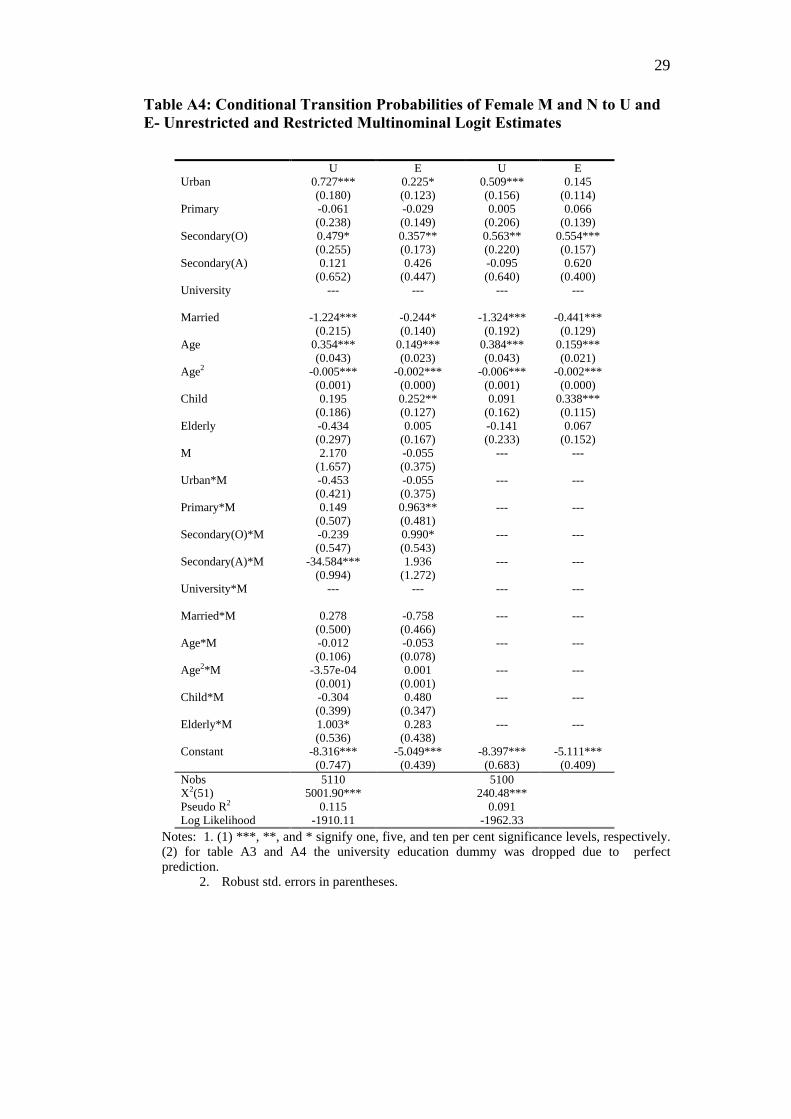
Table A4: Conditional Transition Probabilities of Female M and N to U andE- Unrestricted and Restricted Multinominal Logit Estimates
U E U EUrban 0.727***
(0.180)0.225*(0.123)
0.509***(0.156)
0.145(0.114)
Primary -0.061(0.238)
-0.029(0.149)
0.005(0.206)
0.066(0.139)
Secondary(O) 0.479*(0.255)
0.357**(0.173)
0.563**(0.220)
0.554***(0.157)
Secondary(A) 0.121(0.652)
0.426(0.447)
-0.095(0.640)
0.620(0.400)
University --- --- --- ---
Married -1.224***(0.215)
-0.244*(0.140)
-1.324***(0.192)
-0.441***(0.129)
Age 0.354***(0.043)
0.149***(0.023)
0.384***(0.043)
0.159***(0.021)
Age2 -0.005***(0.001)
-0.002***(0.000)
-0.006***(0.001)
-0.002***(0.000)
Child 0.195(0.186)
0.252**(0.127)
0.091(0.162)
0.338***(0.115)
Elderly -0.434(0.297)
0.005(0.167)
-0.141(0.233)
0.067(0.152)
M 2.170(1.657)
-0.055(0.375)
--- ---
Urban*M -0.453(0.421)
-0.055(0.375)
--- ---
Primary*M 0.149(0.507)
0.963**(0.481)
--- ---
Secondary(O)*M -0.239(0.547)
0.990*(0.543)
--- ---
Secondary(A)*M -34.584***(0.994)
1.936(1.272)
--- ---
University*M --- --- --- ---
Married*M 0.278(0.500)
-0.758(0.466)
--- ---
Age*M -0.012(0.106)
-0.053(0.078)
--- ---
Age2*M -3.57e-04(0.001)
0.001(0.001)
--- ---
Child*M -0.304(0.399)
0.480(0.347)
--- ---
Elderly*M 1.003*(0.536)
0.283(0.438)
--- ---
Constant -8.316***(0.747)
-5.049***(0.439)
-8.397***(0.683)
-5.111***(0.409)
Nobs 5110 5100X2(51) 5001.90*** 240.48***Pseudo R2 0.115 0.091Log Likelihood -1910.11 -1962.33
Notes: 1. (1) ***, **, and * signify one, five, and ten per cent significance levels, respectively.(2) for table A3 and A4 the university education dummy was dropped due to perfectprediction.
2. Robust std. errors in parentheses.

CREDIT PAPERS
98/1 Norman Gemmell and Mark McGillivray, “Aid and Tax Instability and theGovernment Budget Constraint in Developing Countries”
98/2 Susana Franco-Rodriguez, Mark McGillivray and Oliver Morrissey, “Aidand the Public Sector in Pakistan: Evidence with Endogenous Aid”
98/3 Norman Gemmell, Tim Lloyd and Marina Mathew, “Dynamic SectoralLinkages and Structural Change in a Developing Economy”
98/4 Andrew McKay, Oliver Morrissey and Charlotte Vaillant, “AggregateExport and Food Crop Supply Response in Tanzania”
98/5 Louise Grenier, Andrew McKay and Oliver Morrissey, “Determinants ofExports and Investment of Manufacturing Firms in Tanzania”
98/6 P.J. Lloyd, “A Generalisation of the Stolper-Samuelson Theorem withDiversified Households: A Tale of Two Matrices”
98/7 P.J. Lloyd, “Globalisation, International Factor Movements and MarketAdjustments”
98/8 Ramesh Durbarry, Norman Gemmell and David Greenaway, “NewEvidence on the Impact of Foreign Aid on Economic Growth”
98/9 Michael Bleaney and David Greenaway, “External Disturbances andMacroeconomic Performance in Sub-Saharan Africa”
98/10 Tim Lloyd, Mark McGillivray, Oliver Morrissey and Robert Osei,“Investigating the Relationship Between Aid and Trade Flows”
98/11 A.K.M. Azhar, R.J.R. Eliott and C.R. Milner, “Analysing Changes in TradePatterns: A New Geometric Approach”
98/12 Oliver Morrissey and Nicodemus Rudaheranwa, “Ugandan Trade Policyand Export Performance in the 1990s”
98/13 Chris Milner, Oliver Morrissey and Nicodemus Rudaheranwa,“Protection, Trade Policy and Transport Costs: Effective Taxation of UgandanExporters”
99/1 Ewen Cummins, “Hey and Orme go to Gara Godo: Household RiskPreferences”
99/2 Louise Grenier, Andrew McKay and Oliver Morrissey, “Competition andBusiness Confidence in Manufacturing Enterprises in Tanzania”
99/3 Robert Lensink and Oliver Morrissey, “Uncertainty of Aid Inflows and theAid-Growth Relationship”
99/4 Michael Bleaney and David Fielding, “Exchange Rate Regimes, Inflationand Output Volatility in Developing Countries”
99/5 Indraneel Dasgupta, “Women’s Employment, Intra-Household Bargainingand Distribution: A Two-Sector Analysis”
99/6 Robert Lensink and Howard White, “Is there an Aid Laffer Curve?”99/7 David Fielding, “Income Inequality and Economic Development: A
Structural Model”99/8 Christophe Muller, “The Spatial Association of Price Indices and Living
Standards”99/9 Christophe Muller, “The Measurement of Poverty with Geographical and
Intertemporal Price Dispersion”

99/10 Henrik Hansen and Finn Tarp, “Aid Effectiveness Disputed”99/11 Christophe Muller, “Censored Quantile Regressions of Poverty in Rwanda”99/12 Michael Bleaney, Paul Mizen and Lesedi Senatla, “Portfolio Capital Flows
to Emerging Markets”99/13 Christophe Muller, “The Relative Prevalence of Diseases in a Population of
Ill Persons”00/1 Robert Lensink, “Does Financial Development Mitigate Negative Effects of
Policy Uncertainty on Economic Growth?”00/2 Oliver Morrissey, “Investment and Competition Policy in Developing
Countries: Implications of and for the WTO”00/3 Jo-Ann Crawford and Sam Laird, “Regional Trade Agreements and the
WTO”00/4 Sam Laird, “Multilateral Market Access Negotiations in Goods and Services”00/5 Sam Laird, “The WTO Agenda and the Developing Countries”00/6 Josaphat P. Kweka and Oliver Morrissey, “Government Spending and
Economic Growth in Tanzania, 1965-1996”00/7 Henrik Hansen and Fin Tarp, “Aid and Growth Regressions”00/8 Andrew McKay, Chris Milner and Oliver Morrissey, “The Trade and
Welfare Effects of a Regional Economic Partnership Agreement”00/9 Mark McGillivray and Oliver Morrissey, “Aid Illusion and Public Sector
Fiscal Behaviour”00/10 C.W. Morgan, “Commodity Futures Markets in LDCs: A Review and
Prospects”00/11 Michael Bleaney and Akira Nishiyama, “Explaining Growth: A Contest
between Models”00/12 Christophe Muller, “Do Agricultural Outputs of Autarkic Peasants Affect
Their Health and Nutrition? Evidence from Rwanda”00/13 Paula K. Lorgelly, “Are There Gender-Separate Human Capital Effects on
Growth? A Review of the Recent Empirical Literature”00/14 Stephen Knowles and Arlene Garces, “Measuring Government Intervention
and Estimating its Effect on Output: With Reference to the High PerformingAsian Economies”
00/15 I. Dasgupta, R. Palmer-Jones and A. Parikh, “Between Cultures andMarkets: An Eclectic Analysis of Juvenile Gender Ratios in India”
00/16 Sam Laird, “Dolphins, Turtles, Mad Cows and Butterflies – A Look at theMultilateral Trading System in the 21st Century”
00/17 Carl-Johan Dalgaard and Henrik Hansen, “On Aid, Growth, and GoodPolicies”
01/01 Tim Lloyd, Oliver Morrissey and Robert Osei, “Aid, Exports and Growthin Ghana”
01/02 Christophe Muller, “Relative Poverty from the Perspective of Social Class:Evidence from The Netherlands”
01/03 Stephen Knowles, “Inequality and Economic Growth: The EmpiricalRelationship Reconsidered in the Light of Comparable Data”
01/04 A. Cuadros, V. Orts and M.T. Alguacil, “Openness and Growth: Re-Examining Foreign Direct Investment and Output Linkages in Latin America”

01/05 Harold Alderman, Simon Appleton, Lawrence Haddad, Lina Song andYisehac Yohannes, “Reducing Child Malnutrition: How Far Does IncomeGrowth Take Us?”
01/06 Robert Lensink and Oliver Morrissey, “Foreign Direct Investment: Flows,Volatility and Growth in Developing Countries”
01/07 Adam Blake, Andrew McKay and Oliver Morrissey, “The Impact onUganda of Agricultural Trade Liberalisation”
01/08 R. Quentin Grafton, Stephen Knowles and P. Dorian Owen, “SocialDivergence and Economic Performance”

DEPARTMENT OF ECONOMICS DISCUSSION PAPERSIn addition to the CREDIT series of research papers the School of Economicsproduces a discussion paper series dealing with more general aspects of economics.Below is a list of recent titles published in this series.
99/1 Indraneel Dasgupta, “Stochastic Production and the Law of Supply”99/2 Walter Bossert, “Intersection Quasi-Orderings: An Alternative Proof”99/3 Charles Blackorby, Walter Bossert and David Donaldson, “Rationalizable
Variable-Population Choice Functions”99/4 Charles Blackorby, Walter Bossert and David Donaldson, “Functional
Equations and Population Ethics”99/5 Christophe Muller, “A Global Concavity Condition for Decisions with
Several Constraints”99/6 Christophe Muller, “A Separability Condition for the Decentralisation of
Complex Behavioural Models”99/7 Zhihao Yu, “Environmental Protection and Free Trade: Indirect Competition
for Political Influence”99/8 Zhihao Yu, “A Model of Substitution of Non-Tariff Barriers for Tariffs”99/9 Steven J. Humphrey, “Testing a Prescription for the Reduction of Non-
Transitive Choices”99/10 Richard Disney, Andrew Henley and Gary Stears, “Housing Costs, House
Price Shocks and Savings Behaviour Among Older Households in Britain”99/11 Yongsheng Xu, “Non-Discrimination and the Pareto Principle”99/12 Yongsheng Xu, “On Ranking Linear Budget Sets in Terms of Freedom of
Choice”99/13 Michael Bleaney, Stephen J. Leybourne and Paul Mizen, “Mean Reversion
of Real Exchange Rates in High-Inflation Countries”99/14 Chris Milner, Paul Mizen and Eric Pentecost, “A Cross-Country Panel
Analysis of Currency Substitution and Trade”99/15 Steven J. Humphrey, “Are Event-splitting Effects Actually Boundary
Effects?”99/16 Taradas Bandyopadhyay, Indraneel Dasgupta and Prasanta K.
Pattanaik, “On the Equivalence of Some Properties of Stochastic DemandFunctions”
99/17 Indraneel Dasgupta, Subodh Kumar and Prasanta K. Pattanaik,“Consistent Choice and Falsifiability of the Maximization Hypothesis”
99/18 David Fielding and Paul Mizen, “Relative Price Variability and Inflation inEurope”
99/19 Emmanuel Petrakis and Joanna Poyago-Theotoky, “Technology Policy inan Oligopoly with Spillovers and Pollution”
99/20 Indraneel Dasgupta, “Wage Subsidy, Cash Transfer and Individual Welfarein a Cournot Model of the Household”
99/21 Walter Bossert and Hans Peters, “Efficient Solutions to BargainingProblems with Uncertain Disagreement Points”
99/22 Yongsheng Xu, “Measuring the Standard of Living – An AxiomaticApproach”

99/23 Yongsheng Xu, “No-Envy and Equality of Economic Opportunity”99/24 M. Conyon, S. Girma, S. Thompson and P. Wright, “The Impact of
Mergers and Acquisitions on Profits and Employee Remuneration in theUnited Kingdom”
99/25 Robert Breunig and Indraneel Dasgupta, “Towards an Explanation of theCash-Out Puzzle in the US Food Stamps Program”
99/26 John Creedy and Norman Gemmell, “The Built-In Flexibility ofConsumption Taxes”
99/27 Richard Disney, “Declining Public Pensions in an Era of DemographicAgeing: Will Private Provision Fill the Gap?”
99/28 Indraneel Dasgupta, “Welfare Analysis in a Cournot Game with a PublicGood”
99/29 Taradas Bandyopadhyay, Indraneel Dasgupta and Prasanta K.Pattanaik, “A Stochastic Generalization of the Revealed Preference Approachto the Theory of Consumers’ Behavior”
99/30 Charles Blackorby, WalterBossert and David Donaldson, “Utilitarianismand the Theory of Justice”
99/31 Mariam Camarero and Javier Ordóñez, “Who is Ruling Europe? EmpiricalEvidence on the German Dominance Hypothesis”
99/32 Christophe Muller, “The Watts’ Poverty Index with Explicit PriceVariability”
99/33 Paul Newbold, Tony Rayner, Christine Ennew and Emanuela Marrocu,“Testing Seasonality and Efficiency in Commodity Futures Markets”
99/34 Paul Newbold, Tony Rayner, Christine Ennew and Emanuela Marrocu,“Futures Markets Efficiency: Evidence from Unevenly Spaced Contracts”
99/35 Ciaran O’Neill and Zoe Phillips, “An Application of the Hedonic PricingTechnique to Cigarettes in the United Kingdom”
99/36 Christophe Muller, “The Properties of the Watts’ Poverty Index UnderLognormality”
99/37 Tae-Hwan Kim, Stephen J. Leybourne and Paul Newbold, “SpuriousRejections by Perron Tests in the Presence of a Misplaced or Second BreakUnder the Null”
00/1 Tae-Hwan Kim and Christophe Muller, “Two-Stage Quantile Regression”00/2 Spiros Bougheas, Panicos O. Demetrides and Edgar L.W. Morgenroth,
“International Aspects of Public Infrastructure Investment”00/3 Michael Bleaney, “Inflation as Taxation: Theory and Evidence”00/4 Michael Bleaney, “Financial Fragility and Currency Crises”00/5 Sourafel Girma, “A Quasi-Differencing Approach to Dynamic Modelling
from a Time Series of Independent Cross Sections”00/6 Spiros Bougheas and Paul Downward, “The Economics of Professional
Sports Leagues: A Bargaining Approach”00/7 Marta Aloi, Hans Jørgen Jacobsen and Teresa Lloyd-Braga, “Endogenous
Business Cycles and Stabilization Policies”00/8 A. Ghoshray, T.A. Lloyd and A.J. Rayner, “EU Wheat Prices and its
Relation with Other Major Wheat Export Prices”

00/9 Christophe Muller, “Transient-Seasonal and Chronic Poverty of Peasants:Evidence from Rwanda”
00/10 Gwendolyn C. Morrison, “Embedding and Substitution in Willingness toPay”
00/11 Claudio Zoli, “Inverse Sequential Stochastic Dominance: Rank-DependentWelfare, Deprivation and Poverty Measurement”
00/12 Tae-Hwan Kim, Stephen Leybourne and Paul Newbold, “Unit Root TestsWith a Break in Variance”
00/13 Tae-Hwan Kim, Stephen Leybourne and Paul Newbold, “AsymptoticMean Squared Forecast Error When an Autoregression With Linear Trend isFitted to Data Generated by an I(0) or I(1) Process”
00/14 Michelle Haynes and Steve Thompson, “The Productivity Impact of ITDeployment: An Empirical Evaluation of ATM Introduction”
00/15 Michelle Haynes, Steve Thompson and Mike Wright, “The Determinantsof Corporate Divestment in the UK”
00/16 John Beath, Robert Owen, Joanna Poyago-Theotoky and David Ulph,“Optimal Incentives for Incoming Generations within Universities”
00/17 S. McCorriston, C. W. Morgan and A. J. Rayner, “Price Transmission: TheInteraction Between Firm Behaviour and Returns to Scale”
00/18 Tae-Hwan Kim, Douglas Stone and Halbert White, “Asymptotic andBayesian Confidence Intervals for Sharpe Style Weights”
00/19 Tae-Hwan Kim and Halbert White, “James-Stein Type Estimators in LargeSamples with Application to the Least Absolute Deviation Estimator”
00/20 Gwendolyn C. Morrison, “Expected Utility and the Endowment Effect:Some Experimental Results”
00/21 Christophe Muller, “Price Index Distribution and Utilitarian SocialEvaluation Functions”
00/22 Michael Bleaney, “Investor Sentiment, Discounts and Returns on Closed-EndFunds”
00/23 Richard Cornes and Roger Hartley, “Joint Production Games and ShareFunctions”
00/24 Joanna Poyago-Theotoky, “Voluntary Approaches, Emission Taxation andthe Organization of Environmental R&D”
00/25 Michael Bleaney, Norman Gemmell and Richard Kneller, “Testing theEndogenous Growth Model: Public Expenditure, Taxation and Growth Overthe Long-Run”
00/26 Michael Bleaney and Marco Gundermann, “Credibility Gains and OutputLosses: A Model of Exchange Rate Anchors”
00/27 Indraneel Dasgupta, “Gender Biased Redistribution and Intra-HouseholdDistribution”
00/28 Richard Cornes and Roger Hartley, “Rentseeking by Players with ConstantAbsolute Risk Aversion”
00/29 S.J. Leybourne, P. Newbold, D. Vougas and T. Kim, “A Direct Test forCointegration Between a Pair of Time Series”
00/30 Claudio Zoli, “Inverse Stochastic Dominance, Inequality Measurement andGini Indices”

00/01 Spiros Bougheas, “Optimism, Education, and Industrial Development”00/02 Tae-Hwan Kim and Paul Newbold, “Unit Root Tests Based on Inequality-
Restricted Estimators”

Members of the Centre
Director
Oliver Morrissey - aid policy, trade and agriculture
Research Fellows (Internal)
Simon Appleton – poverty, education, householdsAdam Blake – CGE models of low-income countriesMike Bleaney - growth, international macroeconomicsIndraneel Dasgupta – development theoryNorman Gemmell – growth and public sector issuesKen Ingersent - agricultural tradeTim Lloyd – agricultural commodity marketsPaula Lorgelly – health, gender and growthAndrew McKay - poverty, peasant households, agricultureChris Milner - trade and developmentWyn Morgan - futures markets, commodity marketsChristophe Muller – poverty, household panel econometricsTony Rayner - agricultural policy and trade
Research Fellows (External)
V.N. Balasubramanyam (University of Lancaster) – foreign direct investment and multinationalsDavid Fielding (Leicester University) - investment, monetary and fiscal policyGöte Hansson (Lund University) – trade, Ethiopian developmentRobert Lensink (University of Groningen) – aid, investment, macroeconomicsScott McDonald (Sheffield University) – CGE modelling, agricultureMark McGillivray (RMIT University) - aid allocation, human developmentJay Menon (ADB, Manila) - trade and exchange ratesDoug Nelson (Tulane University) - political economy of tradeShelton Nicholls (University of West Indies) – trade, integrationDavid Sapsford (University of Lancaster) - commodity pricesEric Strobl (University College Dublin) – labour marketsFinn Tarp (University of Copenhagen) – aid, CGE modellingHoward White (IDS) - aid, poverty