degree distribution, and scale-free networks
TRANSCRIPT

Degree Distribution,and
Scale-free networks
Prof. Ralucca Gera, Applied Mathematics Dept.Naval Postgraduate SchoolMonterey, [email protected]
Excellence Through Knowledge

Learning Outcomes
Understand the degree distributions of observed networksUnderstand Scale Free networks Power law degree distributionVersus exponential, log-normal, …
2

Degree Distribution
Excellence Through Knowledge

Degree distributions
• The degree distribution is a frequency distribution of the degree sequence
• We define pk to be the fraction of vertices in a network that have degree k
• That is the same as saying: pk is the probability that a randomly selected node of the network will have degree k
• A well connected vertex is called a hub4
p0 1
10, p1
210
, p2 4
10, p3
210
, p4 1
10, pk 0k 5

Plot of the degree distribution
5
• Many nodes with small degrees, few with extremely high– Largest degree is 2407 (not shown). Since 19956
this node is adjacent to 12% of the network
Right-skewed
The Internet Commonly seen plots of real networks

Degree distribution in directed networks
• For directed networks we have both in- andout-degree distributions.
6
The Web

Observed networks are SF (power law)
• Power laws appear frequently in sciences:• Pareto : income distribution, 1897• Zipf-Auerbach: city sizes, 1913/1940’s• Zipf-Estouf: word frequency, 1916/1940’s• Lotka: bibliometrics, 1926• Yule: species and genera, 1924.• Mandelbrot: economics/information theory, 1950’s+
• Research claims that observed real networks are scale free, not consistent defn., [ref. 1–7], i.e. – The fraction of nodes of degree 𝑘 follows a power law distribution
𝑘 , where 𝛼 1, – Generally being observed 𝛼 ∈ 2, 3 , see [ref. 8, 9]– Or at least the upper tail of the distribution is power law) [ref. 10]– Or it is more plausible than other thin-tailed distributions [ref. 11]
Broido and Clauset “Scale-free networks are rare”, Jan 2018, https://arxiv.org/abs/1801.03400 [ref. 13] https://www.eecs.harvard.edu/~michaelm/TALKS/Radcliffe.ppt

Power law distributions
• Power law distribution:(Infinite mean and variance possible)
• Identifying power-law from non power-law distributions is not trivial– Simplest (but not very accurate) strategy visual
inspection plots – In 2006 - fit a distribution over the observed data,
and test the goodness of the fit. This analysis revealed that none of them fits the theoretical distribution
• There are alternatives as we will see8
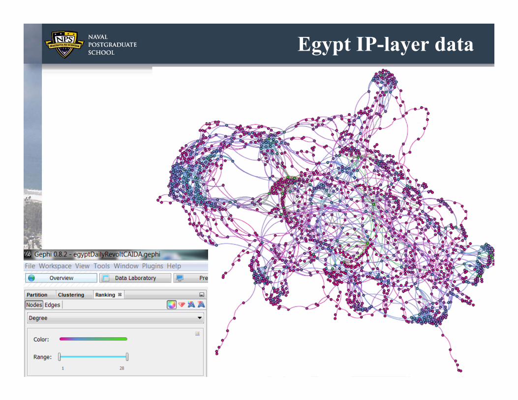
Egypt IP-layer data

And its degree distribution
10A bit hard to differentiate the count values can this visualizationbe improved to be useful? How? We’ll see in a few slides
Notice the long tail.It looks like a power lawdistribution𝑝 𝑐 𝑘 , 𝛼 0

Statistics for real networks
11
α = power in the power law distribution

The powerlaw exponent
12Broido and Clauset “Scale-free networks are rare”, Jan 2018, https://arxiv.org/abs/1801.03400 [ref. 13]
• Claim:𝑝 𝑐 𝑘 , 𝛼 0
• Analysis of 1000 networks: observed networks have the power low exponents plotted on the right
• Code at: https://github.com/adbroido/SFAnalysis

Exponent by network type
13Eikmeier and Gleich, “Revisiting Power-law Distributions in Spectra of Real World Networks”, Aug 2017https://dl.acm.org/citation.cfm?id=3098128
The values of power law exponents for several types of networks

Binning
Excellence Through Knowledge

BA Example (n=1000)
15

Binning
A binned degree histogram may give poor statistics at the tail of the distribution• As k gets large, in every bin there will be only
a few samples large statistical fluctuations in the number of samples from bin to bin which makes the tail end noisy and difficult to decide if it follows a power-law
16

Detecting and visualizing power laws
Alternatives:• We could use larger bins to reduce the noise at
the tail since more samples fall in the same bin– this reduces the detail captured from the histogram
since we end up with fewer bins
17

Logarithmic Binning
Excellence Through Knowledge

Visualizing power laws
Alternatives:• Try to get the best of both worlds different
bin sizes in different parts of the histogram– Careful at normalizing the bins correctly: a bin of
width 10 will get 10 times more samples compared to the previous bin of width 1 divide the count number by 10 logarithmic view (log-log plots)
19
Logarithmic binning
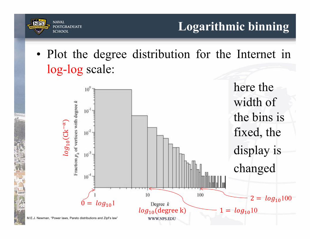
• Plot the degree distribution for the Internet inlog-log scale:
here thewidth ofthe bins isfixed, thedisplay ischanged
0 𝑙𝑜𝑔 11 𝑙𝑜𝑔 10
2 𝑙𝑜𝑔 100
𝑙𝑜𝑔 degree k
𝑙𝑜𝑔
Ck
M.E.J. Newman, “Power laws, Pareto distributions and Zipf’s law”
Logarithmic binning
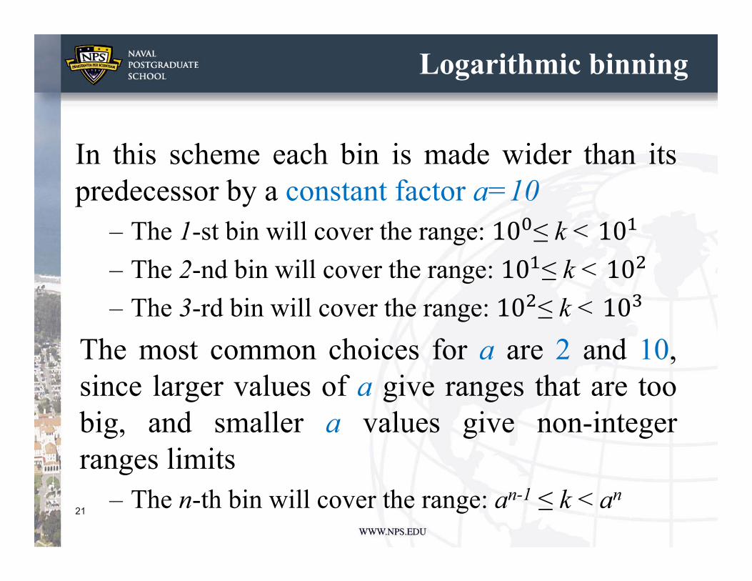
In this scheme each bin is made wider than itspredecessor by a constant factor a=10
– The 1-st bin will cover the range: ≤ k <– The 2-nd bin will cover the range: ≤ k <– The 3-rd bin will cover the range: ≤ k <
The most common choices for a are 2 and 10,since larger values of a give ranges that are toobig, and smaller a values give non-integerranges limits
– The n-th bin will cover the range: an-1 ≤ k < an21

Power Law and Scale Free
Excellence Through Knowledge
Power laws and scale free networks
• Networks that follow power law degree distribution are referred to as scale-free networks
• Scale-free network: means that the ration of very connected nodes to the number of nodes in the rest of the network remains constant as the network changes in size (supports research based on some sampling methods)
• Real networks do not follow power law degreedistribution over the whole range of degree k– That is the degree distribution is not monotonically
decreasing over the whole range of degrees– Many times we refer to its tail only (high degrees)
• Deviations from power law can appear for high values of k as well
http://networksciencebook.com/chapter/4

Power laws and scale free networks
• It is important to mention what property of the network is scale-free.– Generally it is the degree distribution, and we say that
the “network is scale-free” which in reality says “the degree distribution is scale-free”
– Sometimes the exponent of the degree distribution captures this. Why? The exponent is the slope of the line that fits the data on log-log scale.
– This has been tested with random subnetworks of scale free models that indeed show scale free degree distribution (but not always the same exponent)
24

Power law for WWW data from 1999
25
The Degree Distribution of the WWW The incoming (a) and outgoing (b) degree distribution of the WWW (1999). The degree distribution is shown on log-log plot, in which a power law follows a straight line. The symbols correspond to the empirical data and the line corresponds to the power-law fit, with degree exponents γin= 2.1 and γout = 2.45. We also show as a green line the degree distribution predicted by a Poisson function with the average degree ⟨kin⟩ = ⟨kout⟩ = 4.60 of the WWW sample. http://networksciencebook.com/chapter/4#power-laws

Hubs are Large in Scale-free Networks
26http://networksciencebook.com/chapter/4#hubs
The estimated degree of the largest node (natural cutoff) in scale-free and random networks with the same average degree ⟨k⟩= 3. For the scale-free network we chose 𝛼= 2.5. For comparison, we also show the linear behavior, kmax ~ N − 1, expected for a complete network. Overall, hubs in a scale-free network are several orders of magnitude larger than the biggest node in a random network with the same N and ⟨k⟩

A video - scale free property
27http://networksciencebook.com/chapter/4#introduction4

Scale free
Conclusion: in a random network hubs are effectively forbidden, while in scale-free networks they are naturally present. General belief: Scale free networks grow because of preferential attachment• Moreover:
preferential attachment scale free But
preferential attachment scale freecounterexamples: the configuration model, random geometric model
28

New research
Excellence Through Knowledge

New research (Jan 2018) shows:
“over half of the data sets favor the cutoff model over the pure power-law model, which
suggests that, to the degree that scale-free networks are universal, finite-size effects in
the extreme upper tail are quite common”
Broido and Clauset “Scale-free networks are rare”, Jan 2018, https://arxiv.org/abs/1801.03400 [ref. 13]
(Power law is a specific instance of this power law with cuttoff)
Example:“exponential distribution, which exhibits a thin tail and relatively low variance, is favored over the power law (36%) nearly as often as the power law is favored over the exponential (37%).”
Power law

Takeaways
• Networks have heavy-tailed degree distributions: – scale-free networks are rare: 4% strong SF, and – 33% weak (as likely as other models) SF evidence
• Weak correlation of SF across different types:– Stronger correlation shows that SF structures occur in
biological and technological networks• “…there is likely no single universal mechanism,
or even a handful of mechanisms, that can explain the wide diversity of degree structures found in real-world networks.”
31Broido and Clauset “Scale-free networks are rare”, Jan 2018, https://arxiv.org/abs/1801.03400 [ref. 13]

References
[1] R. Albert, H. Jeong, and A. L. Barab´asi, Nature 401, 130 (1999).[2] N. Prˇzulj, Bioinformatics 23, 177 (2007).[3] G. Lima-Mendez and J. van Helden, Molecular BioSystems 5, 1482 (2009).[4] A. Mislove, M. Marcon, K. P. Gummadi, P. Druschel, and B. Bhattacharjee, in Proc. 7th ACM SIGCOMM Conference on Internet Measurement (IMC) (2007) pp. 29–42.[5] M. T. Agler, J. Ruhe, S. Kroll, C. Morhenn, S. T. Kim, D. Weigel, and E. M. Kemen, PLoS Biology 14, 1 (2016).[6] G. Ichinose and H. Sayama, Artificial Life 23, 25 (2017).[7] L. Zhang, M. Small, and K. Judd, Physica A 433, 182 (2015).[8] S. N. Dorogovtsev and J. F. F. Mendes, Advances in Physics 51, 1079 (2002).[9] A. L. Barab´asi and R. Albert, Science 286, 509 (1999).[10] W. Willinger, D. Alderson, and J. C. Doyle, Notices of the AMS 56, 586 (2009).[11] R. Albert, H. Jeong, and A.-L. Barab´asi, Nature 406, 378 (2000).[12] N. Eikmeier, and D. Gleich. "Revisiting Power-law Distributions in Spectra of Real World Networks." Proceedings of the 23rd ACM SIGKDD International Conference on Knowledge Discovery and Data Mining. ACM, 2017.[13] A. Broido and A. Clauset, “Scale-free networks are rare”, 2018
32

New research (Jan 2018) data:
• Applying state-of-the-art statistical methods to a diverse corpus of 927 real-world networks:– estimate the
best-fitting power-law model,
– test its statistical plausibility, and
– compare it via a likelihood ratio test to alternative non-scale-free distributions.
33Broido and Clauset “Scale-free networks are rare”, Jan 2018, https://arxiv.org/abs/1801.03400 [ref. 13]
Best fitting model
1. For each degree sequence, estimate the best-fitting power-law distribution model: the power-law holds above some minimum value 𝑘 , chosen
before fitting the distributionTest use is Kolmogrov-Smirnov (KS) minimization approach
(which actually chooses the optimal value of 𝑘 )
2. Used goodness-of-fit to obtain a standard p-value: if p ≥ 0.1, then the degree sequence is scale free, while
if p < 0.1, reject the scale-free hypothesis. failing to reject does not imply that the model is correct, only
that it is a plausible data generating process. 34
Broido and Clauset “Scale-free networks are rare”, Jan 2018, https://arxiv.org/abs/1801.03400 [ref. 13]

Testing the goodness-of-fit
Alternative heavy tailed distrib. (starting at ): Exponential (a thin tail and relatively low variance),
stretched exponential or Weibull distribution (can produce both thin or heavy tails, and is a generalization of the exponential distribution),
log-normal (a broad distribution that can exhibit very heavy tails, finite mean and variance),
power-law with exponential cutoff in the upper tail (power law is a special case of this).
35
Broido and Clauset “Scale-free networks are rare”, Jan 2018, https://arxiv.org/abs/1801.03400 [ref. 13]

Comments from papers
• “If real-world networks are not universally or even typically scale-free, the status of a unifying theme in network science over nearly 20 years would be significantly diminished. Such an outcome would require a careful reassessment of the large literature that has grown up around the idea.”
• “Hence, an important direction of future work in network theory will be development and validation of novel mechanisms for generating more realistic degree structure in networks”
36Broido and Clauset “Scale-free networks are rare”, Jan 2018, https://arxiv.org/abs/1801.03400 [ref. 13]