delay time analysis in maintenance

Delay Time Analysis

in Maintenance

A Thesis submitted for the Degree of

Doctor of Philosophy

by

David Francis Redmond

Research Institute for Technology, Information,

Management and Economics

Department of Mathematics and Computer Science

University of Salford

1997

11

, Abstract

The thesis develops the application of delay time analysis to the area of

mathematical modelling of planned maintenance and inspection of industrial systems. Chapter 1 gives an introduction to the history and

techniques in use of maintenance modelling and surveys appropriate literature in the field. A section is devoted to papers published on delay

time analysis. Chapter 2 introduces and develops mathematical models for

modelling the reliability, maintenance and inspection of repairable

systems. Chapter 3 gives an account of parameter estimation and model

updating techniques in the light of subjective and observational data sets

collected over a period of system operation. Chapter 4 addresses a bias

in the probability distribution function of delay time when the data

available over an operating survey is censored. Parameter estimation

methods for this situation are then proposed. Chapter 5 gives an account

of a simulation study of the delay time models and verifies the theory and

parameter estimation techniques. Chapter 6 reports on research supported

by the Science and Engineering Research Council on the application of delay

, time analysis to concrete structures. Finally, Chapter 7 collates the

conclusion drawn on each chapter and recommends areas for further

research.

iii

Contents

Page

Abstract ii

Acknowledgements viii

Chapter 1: Introduction and Literature Review

1.1 Introduction 1

1.2 Maintenance Modelling of Single Components 2

1.2.1 Renewal theory and reliability 3

1.2.2 Models for cost 6

1.2.3 Models for downtime 8

1.2.4 Estimation of modelling parameters 9

1.3 Maintenance Modelling of Systems 12

1.3.1 Stochastic processes 12

1.3.2 Models for cost 14

1.3.3 Modelling downtime 15


1.4 Delay Time Inspection Modelling 16

1.4.1 Review of papers 18

1.4.2 Single-component models 20

1.4.3 System models 23


1.4.5 Introduction to chapters 26

1.5 Discussion 32

iv

Chapter 2: Delay Time Models for Maintenance of a Repairable System

2.1 Introduction 35

2.2 Delay Time Concept for a Repairable System 35 2.3 Type of Maintenance Activities 38

2.4 Failure Based Maintenance (FBM) 38

2.4.1 Number of breakdowns arising over time 39

2.4.2 Modelling cost 41


2.4.4 Non-homogeneous defect arrivals 44

2.5 Periodic Based Inspection (PBI) 45

2.5.1 The probability a defect causes a breakdown 47


2.5.3 Modelling cost 50

2.5.4 Perfect inspection models with non-homogeneous 53

defect arrivals 2.5.5 Imperfect inspection models with homogeneous 54

defect arrivals 2.6 Use Based Inspection (UBI) 57

2.7 Exponential Delay Time Example 59

2.8 Conclusion 61

Chapter 3: Parameter Estimating and Updating for

Delay Time Models

3.1 Introduction 63

3.2 Assumptions and Data 64

3.3 Need to Update Prior Model 67

3.4 Updating Procedure 69

V

3.5 Linear Delay Time Update 70

3.5.1 Special case, scale parameter, a, update 72

3.5.2 Special case, shift parameter, w, update 75

3.5.3 General linear case 76

3.6 Model Parameter Variation 78

3.6.1 Combining the methods 79

3.7 Criteria for Choosing Method of Updating 80

and Estimating

3.7.1 Method of moments parameter selection 81

3.7.2 Maximum likelihood parameter selection 82

3.8 Statistical Tests of Fit 84

3.9 Other Updating Methods 85

3.10 Decision Consequence 85

3.11 Conclusion 87

Chapter 4: Bias in Delay Time and Initiation Time Parameter

Estimates for Censored Data

4.1 Introduction 89

4.2 Bias in Delay Time Parameter Estimates 89

4.2.1 Delay times associated with breakdowns 91

4.2.2 Delay times associated with 93

inspected defects

4.3 Bias in Initiation Time Parameter Estimates 96

4.4 Imperfect Inspections (ß # 1) 98

4.4.1 Initiation times when ß#1 100

4.5 Correcting for Bias in Parameter Estimates of 101

Delay Time and Initiation Time

vi

4.5.1 Perfect inspections, ßo =1 102

4.5.2 Imperfect inspections, (30 #1 104

4.6 Additional Tests of Model Fit 105

4.7 Conclusion 105

Chapter 5: Simulation Study of the Delay Time Model

5.1 Introduction 106

5.2 Pilot Simulation of the Delay Time Model 107

5.2.1 Perfect inspections 107

5.2.2 Imperfect inspections 111

5.3 Simul ation over a Series of Inspections 114

5.3.1 Perfect inspections 114

5.3.2 Imperfect inspections 117

5.3.3 Non-instantaneous breakdown repairs 118

5.4 Estimation Techniques using Simulated Data 120

5.4.1 Correcting for bias in delay time parameter estimates 120

5.4.2 Updating option 121

5.4.3 Iteration method to capture scale and 124

shape parameters 5.4.4 Criteria for deciding on whether to accept 126

the updated model 5.4.5 Estimating using the observed breakdown times 127

5.5 Conclusion 128

Chapter 6: Application of Delay Time Analysis to Concrete

Structures

6.1 Introduction

6.2 Deterioration of Concrete Structures

130

131

vii

6.3 Data Collection and Analysis 133

6.4 Modelling Deterioration of a Component 136

6.4.1 Maximum likelihood estimation 138

6.4.2 Estimation on real data 140

6.4.3 Test of model fit 141

6.5 Maintenance Models of Cost 147

6.5.1 Single-component cost models 149

6.5.2 Multi-component cost models 152

6.6 Conclusion 155

Chapter 7: Conclusion

7.1 Literature Review 158

7.2 Delay Time Models for Maintenance of a 159

Repairable System

7.3 Parameter Updating and Estimating for 160

Delay Time Models

7.4 Bias in Delay Time and Initiation Time Parameter 161

estimates for Censored Data

7.5 Simulation Study of the Delay Time Model 162

7.6 Application of Delay Time Analysis to Concrete Structures 163

Appendix : Stochastic case model for downtime 166

References 168

viii

Acknowledgements

I wish to thank my supervisor, Professor A. H. Christer, for the

opportunity to contribute to this challenging area of research and for

providing the necessary assistance, insight and support needed to achieve

successful results.

I acknowledge colleagues I have met at the University of Salford and

other institutions working in the field of operational research and

maintenance modelling for supplementing my understanding and

perception of the research.

Special thanks to my parents, family and all my friends for providing help, support and motivation necessary to complete the work.

Chapter 1

Introduction and Literature Review

1.1 Introduction

The demand for effective maintenance modelling and use of operational research (OR)

to this end is evident in the recorded experiences of World War II, see Waddington

(1973), OR in World War II: OR against the U-boat. Khintchine (1932) was one of first

contributors to attempt to mathematically model machine maintenance. Since then, the

field of planned maintenance for plant and buildings has received considerable interest

and attention due to the increasing complexity of machinery and building designs, and

the necessity for such systems to perform their function optimally in terms of cost,

downtime and reliability. Stochastic modelling and statistical analysis have underpinned

much of the OR methodology used for attempting to model and predict the

consequences to and behaviour of equipment when maintenance strategies are applied.

Informative accounts and reviews of mathematical techniques applied to maintenance

are given by; Cox (1957), Barlow and Proschan (1965), McCall (1965), Jardine (1973),

Pierskella and Voelker (1976), Christer (1984), Ascher and Feingold (1984), Barlow

(1984), Thomas (1986), Valdez-Flores and Feldman (1989), Cho and Parlar (1991),

Thomas et al (1991), Baker and Christer (1994).

This chapter proceeds by modelling single component items such as, for example, light

bulbs, where usually it makes sense to assume that only one type of failure can be

experienced. Models for reliability, cost and downtime consequences given maintenance

options are then discussed along with the necessary statistical analysis and estimation

techniques. Modelling procedures applied to systems of components are then addressed. In the fourth section, the concept of delay time analysis applied to maintenance and

2

inspection (the subject of the thesis), introduced by Christer (1973), is reviewed. The

research undertaken in the thesis is introduced. Finally, an overall discussion concludes

the chapter.

1.2 Maintenance Modelling of Single Components

A component (or part) is a device that can fail in one failure mode when in operation

and providing its service. Examples include light bulbs, valves and fuses. Failure is the

state such that the component needs repair or complete replacement. The consequence

of failure will induce costs due to repair or replacement. A period of downtime will be

incurred until the component is restored and operating. The downtime required to

replace the item will either be known prior to replacement/repair or possibly unknown.

Indeed, penalty costs such as, for example, lost production, due to the component being

out of service could also be incurred.

A maintenance strategy or concept is a set of directives (or policies) aimed at optimising

an objective function, e. g cost or downtime, over a period of time. The set of policies

considered may be constrained so that certain operating characteristics are achieved, e. g

a guaranteed reliability performance. One such policy could be simply to restore failed

components as they arise, that is Failure Based Maintenance (FBM). Another strategy

could be to replace components after a determined period of operation or at failure,

whichever comes first, and is an example of a planned preventive maintenance (PPM)

policy. The period of failure free operation is the decision parameter in the model. In

some cases, a component may not signal immediate failure to the operator, e. g standby

devices and the deterioration to a defined failed state in concrete structures. These types

of components would require an inspection or monitoring type policy.

Many components may become defective prior to failure and still remain operable, e. g

a strip-light would flicker and take more time to switch on in the latter stage of its life.

These types of components may benefit from an inspection policy whereby a component

is inspected for the defect and consequently replaced at inspection to prevent failure.

The time to inspect is the decision parameter. The defective phase would need to be

included in a maintenance model. Delay time modelling has provided a tool for

3

modelling the consequence of maintenance and inspection for components of this type.

In recent years, condition monitoring techniques have been developed. A component can

be continuously or periodically monitored for engineering factors, e. g stress or vibration.

A decision on replacement/repair can then be made when a particular factor reaches a

certain threshold.

1.2.1 Renewal Theory and Reliability

The classic methodology for modelling the maintenance of single components is the

application of renewal theory and reliability. Cox (1957) and Barlow and Proschan

(1965) give excellent accounts of this field of mathematics. The approach is to assume

that each component has its time to failure, X say, governed by a probability law, that

is X is distributed with an assumed probability density function (p. d. f), f(x) say.

When a component is replaced, which may be at failure, it is then assumed that the

replaced component then operates independently and statistically identical to its

predecessor, in other words, a renewal point. It is also possible that a component can

be repaired to an assumed 'as-new' state which is statistically equivalent to a renewal.

The independence assumption, in this case, would need to be tested.

The FBM policy for a single component is an example of a renewal process, whereby

the operating time between each failure is assumed to be independent and identically

distributed (i. i. d) with p. d. f of time to failure, ix). The reliability, R(x) say, of a

component is the probability that the component will operate without failure over time

interval (0, x) measured from when the component was assumed new and placed in

operation. The reliability function, R(x), is simply given by the probability that the

failure time exceeds x, that is to say,

w R(x) =

ff(y)dy =1- F(x)

yax

where F(x) is the cumulative distribution function (c. d. f) of X. The mean time to failure

(MTTF), µ= E(X) say, is given by,

4

w N=f xf(x) dr

=o _

JR(x)dx (1.2)

The hazard rate, z(x) say, is a function such that in the small interval (x, x+d:: ), z(x)dx,

is the probability that the component will fail given it has not caused a failure over the

operating time interval (0, x), since last new, i. e P{X c (x, x+ dx) IX> x}, where X is

the random time to failure. It follows that z(x) is given by,

Z(X) - fix) R(x)

(1.3)

The functions f(x) and R(x) can be written uniquely as a function of the hazard rate, z(x),

see Cox (1957, p. 5). This can be shown by formulating the cumulative hazard function,

Z(x) say, that is the integral of z(x), given by,

x

Z(x) =f) dv = -ln(R(x)) (1.4)

r=o R(')

Hence, R(x) = exp(-Z(x)) and f(x) = z(x)exp(-Z(x)). It can be seen that a component

with a constant hazard rate, whereby the instantaneous chance of failure does not change

with operating time, has an exponential distribution of time to failure.

Typical lifetime distributions commonly selected for components are exponential,

Weibull, Erlang, gamma and lognormal. Depending on the selected distribution, the

hazard rate, for example, could be monitonically increasing, whereby the chance of

failure in the next instance of component operation, given no prior failure, increases as

the component operates, i. e the component is such that it is wearing out. A decreasing

hazard applies to components which become increasingly reliable as they operate

without failure, e. g computer chips. It has been a common assumption that many

component types have a 'bath-tub' hazard which decreases at first. This to allow for a

sub-set of components to be possibly defective through manufacture, and having infant

mortality. Then, the hazard is assumed approximately constant for a certain time

(sometimes termed main life), and finally increasing (wear out).

The sample hazard function would be formed from the life testing of a set of

5

components. Analysis of the failure behaviour of a component, say through condition

monitoring or inspection, may reveal that a component becomes defective, giving a

signal that it is about to fail or has an increasing chance of failure. In this case, the bath-

tub assumption would not be appropriate as a basis for modelling this effect. An

inspection would naturally increase or decrease the hazard function of failure, for

component operation immediately after inspection, depending if a defect is found or not

found. The defective property of the component would need to be included in a

maintenance model. Delay time analysis provides a model to take this effect into

account.

It is of interest in maintenance modelling to estimate the expected number of

breakdowns, B(T) say, over an interval (0,7). For the renewal process, B(7), is given

by the solution to the renewal equation,

T

B(T) = F(T) +f B(T - x) f(x) dx

x0 (1.5)

_ F'k'(T k=1

where Fk'(x) is the k-fold convolution of F(x), that is the c. d. f of time to the k'th failure.

We shall also define, here, r(7), as the instantaneous rate of occurrence of failures

(ROCOF), given by,

r(T) = B'(7) , f'(k)(7)

k=1

(1.6)

where Ik'(x) is the p. d. f of time to the k'th failure. The ROCOF and hazard rate has

caused much confusion in the reliability field, see Ascher and Feingold (1984). The

ROCOF is an absolute rate of the stochastic process of failures from the origin of the

process. The hazard rate is relative, in that it is a direct property of the time between

two failures. A consequence of the renewal process, is that in the limit as time increases,

1Tm- B(_ = tim-r(7) _ (1.7)

and for large T and finite variance, & say, of time to failure, B(7) = T/µ + ((Y2 - µ2)/2µ2,

6

see Cox (1957, p. 47, p. 55). This implies the process becomes steady state, for example

the expected number of failures in an interval, (T,, T2) say, selected prior to the process

starting, would be approximately (T2 - T1)! µ for large values of Ti and T2. The time

taken' to reach this state will depend on the selected p. d. f of time to failure.

The functions introduced in this section are some of the characteristics of the behaviour

of a single component system, and are important in the maintenance modelling and the

estimation and testing of modelling parameters. However, it has been highlighted that

properties of defects of a component would also be an important ingredient in

maintenance modelling, and will prove to be so in the forthcoming chapters on delay

time analysis.

1.2.2 Models for Cost

We, here, introduce two models of cost and refer to literature on other cost model

structures. Jardine (1973) gives an account of many models for single-component

systems. The two common types are block and age based replacement.

Block replacement can apply to a single or group of like components. The policy is to

replace the component(s) at periodic points in time, T, 2T, ...,

NT, say. The decision

parameter for the model is clearly T. Components which fail over the replacement

periods are assumed to be replaced at failure with a statistically identical component. Let

cf be the expected cost of replacing a failed component and c, (< cf) be the expected cost

of a planned replacement. It is also assumed that a failure and planned replacement is

carried out with negligible time. For one component, the expected cost over each

replacement cycle is Cr + cfB(T). Hence, the expected cost per unit time, c(T) say, over

each cycle is given by,

G(7) _ Cl + `" fB(T) (1.8)

T

For a group of, M say, like components the expected cost would simply be multiplied by M. Also, a block replacement downtime, for this case, dr say, may need to be

considered in the denominator of c(7). By differentiating c(T), the optimum solution, if

it exi ; ts, can be found by solving the equation,

7

cf(r(T) - BT))

- C, =0 (1.9)

Using the limiting results of the renewal process in the previous section, failure-based

maintenance has an expected cost per unit time, c/µ, and the block replaceme, lt strategy

would have a solution to equation (1.9) with a lower expected cost per unit time

if cJcf < (62 - p2)/2p, assuming the absence of technological improvement or condition

monitoring. Dagpunar (1994) tidies up the necessary and sufficient conditions for

optimality based on the mean residual life property of the failure p. d. f, Ax). A

disadvantage of the model is that failures may occur just before a planned replacement.

Hence, the policy would apply to mainly inexpensive items, such as light-bulbs.

In age-based replacement, each component is replaced at failure or when attaining age

T, whichever comes first. Hence, each component's age needs to be monitored for the

application of this policy. We will assume that each component has failure and

preventive replacement expected costs, cf, c1 respectively. The replacement cycle will

end at failure or T. Hence, the expected cost per cycle is cfF(T) + c, R(T). The cycle

length is clearly random, and its expectation, m(T) say, will be given by,

TT

nl(T) =f xf(x)dx + TR(T) = 5R(x)dx

. (1.10)

xo x0

The expected cost per unit time, c(7), over a finite time horizon may be complex

involving the use of renewal functions. Using renewal theory, the long term expected

cost per unit time is given by the ratio of the expected cost to the expected cycle length,

see Cox (1957, p. l 18). Hence, c(7), for one component is given by,

c1F(T) + crR(T)

Again, a group, size M, of components would have expected cost per unit time, Mc(7).

An optimal solution, if it exists, can be found graphically or by differentiating,

simplifying and solving the equation,

8

T

(Cf - cT) z(T) f R(x) dx - F(T) - Cr =O (1.12)

x=0

where z(x) is defined in function (1.3). When considering the L. H. S at T= oo, it can be

seen that a uniquie solution will exist, if pz, (°°) > c/(cf - cr) and z(x) is strictly increasing

, since the L. H. S is negative at T= 0 and is monitonically increasing. Dagpunar (1994)

discusses further the conditions for the existence and uniqueness of an optimum. It is

must be noted that the optimal age-based or block replacement solution may not be the

overall optimum maintenance strategy for the component, in that other strategies through

use of inspections or condition monitoring may provide lower cost per unit time. This

will be shown in Section 1.4.2

The following papers give characteristive examples of cost models. Beichelt (1981)

considers a model where detection of failure can only be made by inspection. An

increasing cost between failure and inspection is considered and an optimal irregular

spaced inspection strategy is proposed. This is a similar situation to the modelling of

concrete structures in Chapter 6. Christer and Keddie (1985) present a replacement

model applied to filling valves on a canning line. Kaio and Osaki (1989) compare

inspection policies for a component that can only be detected as failed by inspections.

Jack (1991) considers the effect of imperfect repairs over finite time horizons. Makis

and Jardine (1992) consider also a replacement and repair cost model, which takes into

account the possibility of imperfect repair. Dagpunar (1994) extends the age-based

replacement cost model by introducing non-zero downtimes for failure and planned

replacement. Necessary and sufficient conditions are formulated and discussed. An

example is given in the paper, based on a case study, in Christer and Keddie (1985). A

recent application study has been published, see Vanneste and Wassenhove (1995).

1.2.3 Models for Downtime

Modelling downtime for maintenance strategies can become complex due to

incorporating the finite time for renewing a component within a stochastic model. Barlow and Proschan (1965) and Barlow and Hunter (1960b) model the failure-repair

9

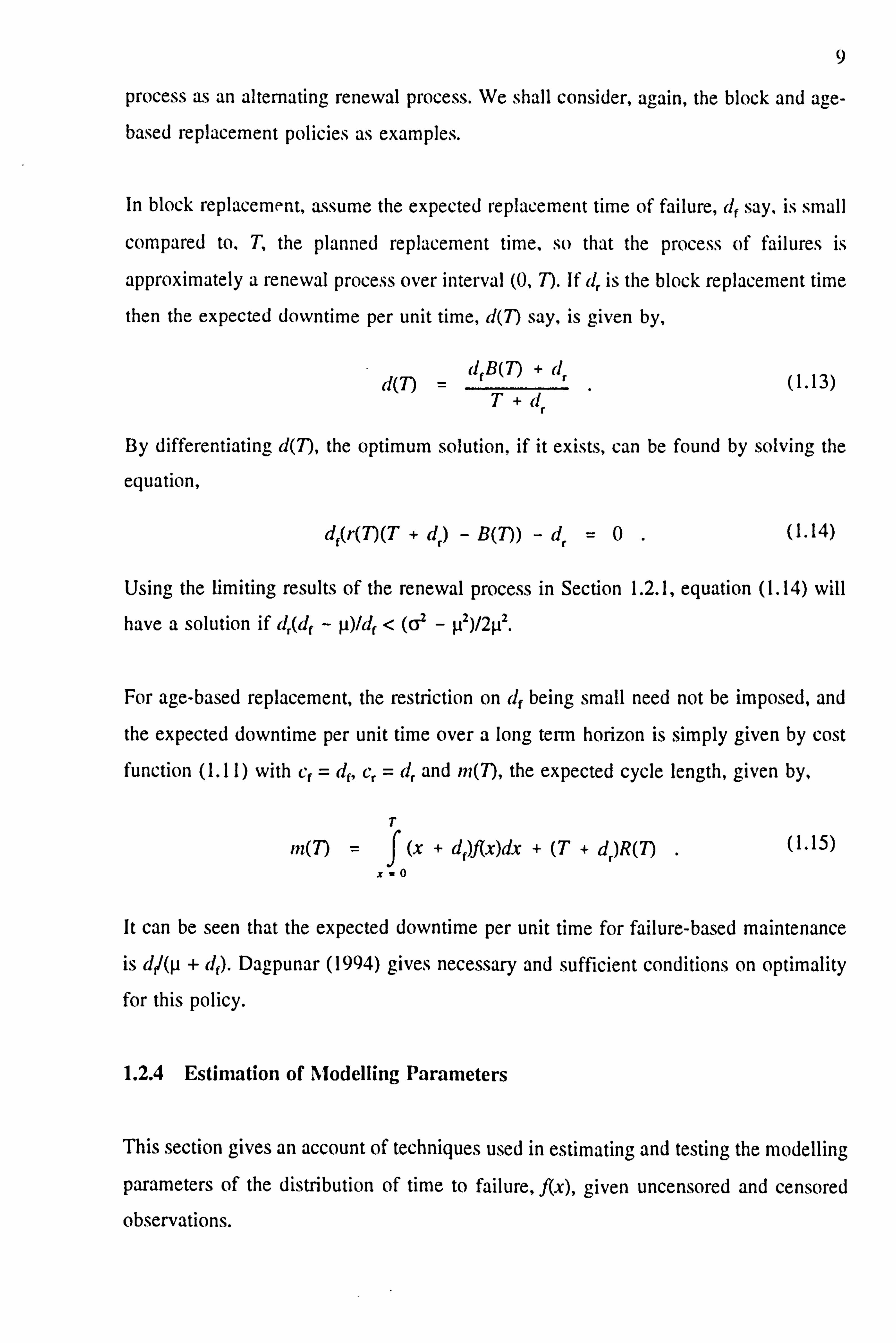
process as an alternating renewal process. We shall consider, again, the block and age- based replacement policies as examples.

In block replacement, assume the expected replacement time of failure, df say, is small

compared to, T, the planned replacement time, so that the process of failures is

approximately a renewal process over interval (0,7). If dr is the block replacement time

then the expected downtime per unit time, d(T) say, is given by,

d(7) _ cl fB(T) + dý

. T +d, (1.13)

By differentiating d(T), the optimum solution, if it exists, can be found by solving the

equation,

d f(r(7)(T + dr) - B(7)) - d, =0. (1.14)

Using the limiting results of the renewal process in Section 1.2.1, equation (1.14) will have a solution if dr(d f- µ)/df < (a2 - µ2)/2µ2.

For age-based replacement, the restriction on df being small need not be imposed, and

the expected downtime per unit time over a long term horizon is simply given by cost

function (1.11) with cf= df, Cr = dr and m(T), the expected cycle length, given by,

11z(7) =f (x +d f)f(z)dx + (T + dr)R(n . (1.15)

0

It can be seen that the expected downtime per unit time for failure-based maintenance is d/(µ + (if). Dagpunar (1994) gives necessary and sufficient conditions on optimality for this policy.

1.2.4 Estimation of Modelling Parameters

This section gives an account of techniques used in estimating and testing the modelling

parameters of the distribution of time to failure, f(x), given uncensored and censored

observations.

10

Assume N independent components of the same type are placed in operation and each

one is run to failure, with x; say, being the observed time to failure of the i'th

component, 1 <_ i5N. The components need not necessarily be placed in operation at

the same time. It is also assumed, for now, that the set {x, } do not form a series of

events generated by repairs to a single component. The following sample functions can

easily be calculated; probability histogram, c. d. f, reliability function, hazard and

cumulative hazard. This aids in deciding the form of the p. d. f, f(x), of x. Statistics such

as the sample mean and variance can be calculated and confidence limits can be placed

on the theoretical values of these parameters.

We now consider estimation techniques. Two formal methods of estimation are in

common use, that is maximum likelihood and method of moments. Assume the p. d. f

family selected has form f(x; 1) where X is the set of parameters to be estimated. The

likelihood function of the data set {x, } is given by,

N

LQ) _ ll f(xý; 2, (1.16)

which represents a probabilistic measure of observing the given observations. The

estimated parameters are chosen at the point such that L(j) (or alternatively, Ln(L(2)),

the log-likelihood) is a maximum.

For the method of moments estimation, the first M sample moments about x=0 are

calculated, where M is the number of parameters to be estimated. Then, M simultaneous

equations are set up by equating each sample moment to the corresponding theoretical

moment, see Chatfield (1970, p. 121). It follows that the following equations would need

to be solved,

fxif(x; x)dx = for for 1 <_ j <_ M (1.17) X=0 i-1

These equations can then be solved, if a solution exists, to obtain a point estimate of I.

In testing the fit of the model, the sample probability histogram can be compared to the

estimated histogram and the x` test can be undertaken. Alternatively, the sample and

estimated c. d: f can be compared and the Kolmogorov-Smirnoff (KS) test can be carried

out.

We next discuss the situation of censored observations in the context of block and age-

based replacement policies. Assume, T is the current replacement practice for either

policy. Over an operating survey, two sets of data on failures would arise, that is a set

of size, A say, completely observed times to failure and a set of size, B say, of censored

times (due to replacement at 7), where it is only known the time of failure exceeds a

specific value. We shall denote these sets, {. x; }, 1 <_ j <_ A, and {Yk}, 1 _<

k <_ B. The

maximum likelihood estimation can also be applied, and is given by,

AB

L( )_ý xýý)T7R(yk; X) (1.18)

For age-based replacement, all the censored values, yk. will be equal to T, and a test-of-

fit can be carried out using the conditional c. d. f of x over the interval (0, T), that is

F(x)/F(T), and comparing it to the sample c. d. f of failure times. Additionally, the sample

proportion of planned replacements can be compared to the estimated reliability,

P{x > T} = R(T), and a binomial statistical test carried out. For the block-replacement

case (or progressively censored samples, in general, where the set {yk} have random

values), a graphical test-of-fit can be undertaken using the cumulative hazard function,

see Nelson (1984), and a statistical test-of-fit undertaken by using the Kaplan-Meier

estimate of the reliability function, see Kalbfleisch and Prentice (1980).

The procedures outlined above, will be applied to delay time analysis, in the appropriate

modified forms, for simulated data in Chapter 5, and on the analysis of inspection

records of concrete components in Chapter 6.

When considering repairs to a single component, and {x; } is the set of inter-arrival times

of failures, then a trend could be seen by plotting cumulative failures versus operating

time. An increasing gradient would show deterioration whilst a decreas; ng gradient

would show component improvement. In these cases, the component may not always be

repaired to 'as-new', and the times {x; } may not be independent and identically

distributed, see Ascher and Feingold (1984). A renewal process is then not appropriate

and the estimation techniques above would not apply. The next section on systems

12

presents one model which can cope with this effect.

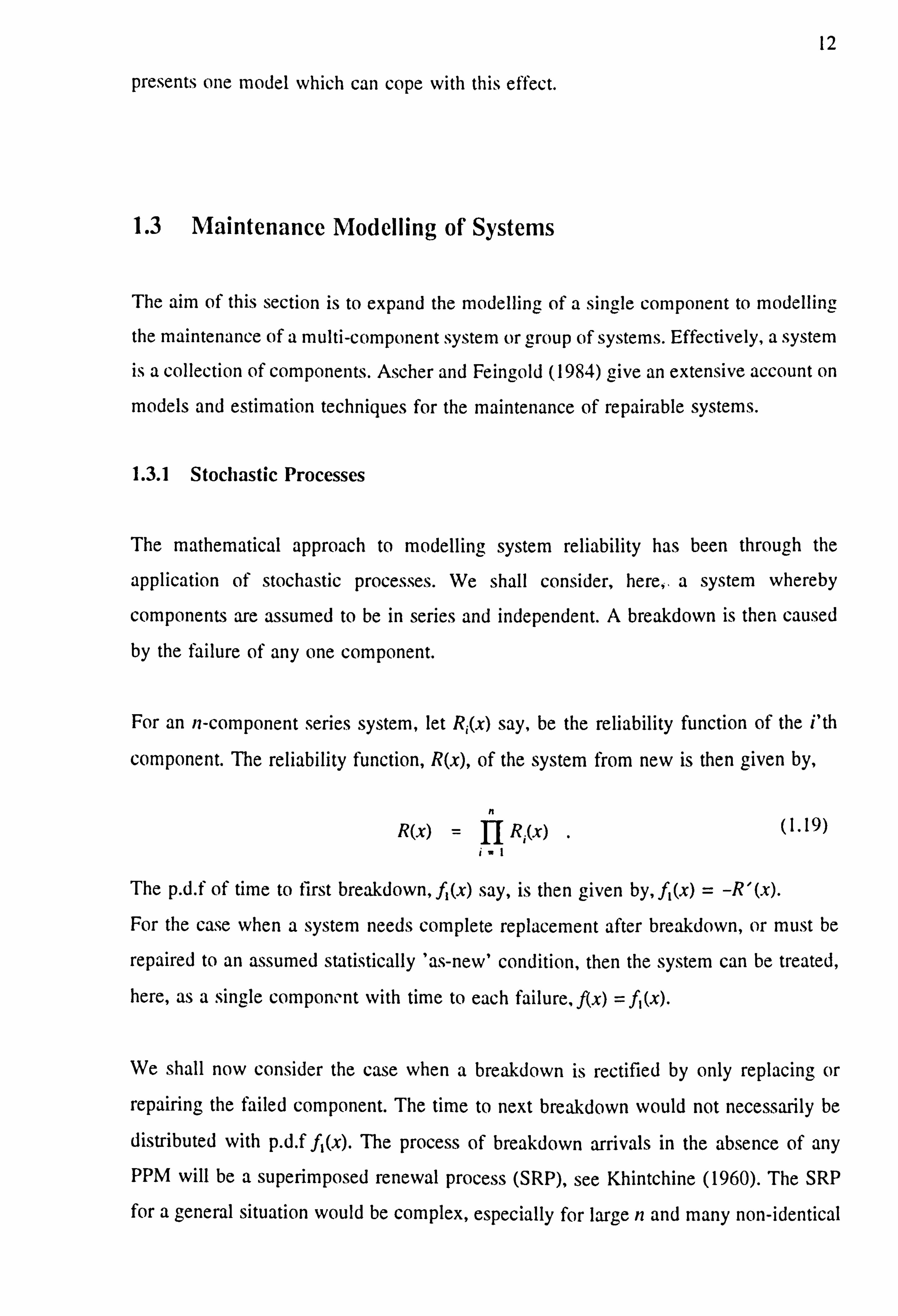
1.3 Maintenance Modelling of Systems

The aim of this section is to expand the modelling of a single component to modelling

the maintenance of a multi-component system or group of systems. Effectively, a system

is a collection of components. Ascher and Feingold (1984) give an extensive account on

models and estimation techniques for the maintenance of repairable systems.

1.3.1 Stochastic Processes

The mathematical approach to modelling system reliability has been through the

application of stochastic processes. We shall consider, here,. a system whereby

components are assumed to be in series and independent. A breakdown is then caused

by the failure of any one component.

For an n-component series system, let R; (x) say, be the reliability function of the i'th

component. The reliability function, R(x), of the system from new is then given by,

n

R(x) = ll R, (x) (1.19) i1

The p. d. f of time to first breakdown, f, (x) say, is then given by, f, (x) = -R'(x). For the case when a system needs complete replacement after breakdown, or must be

repaired to an assumed statistically 'as-new' condition, then the system can be treated,

here, as a single component with time to each failure, f(x) = f, (x).

We shall now consider the case when a breakdown is rectified by only replacing or

repairing the failed component. The time to next breakdown would not necessarily be

distributed with p. d. f fi(x). The process of breakdown arrivals in the absence of any PPM will be a superimposed renewal process (SRP), see Khintchine (1960). The SRP

for a general situation would be complex, especially for large n and many non-identical

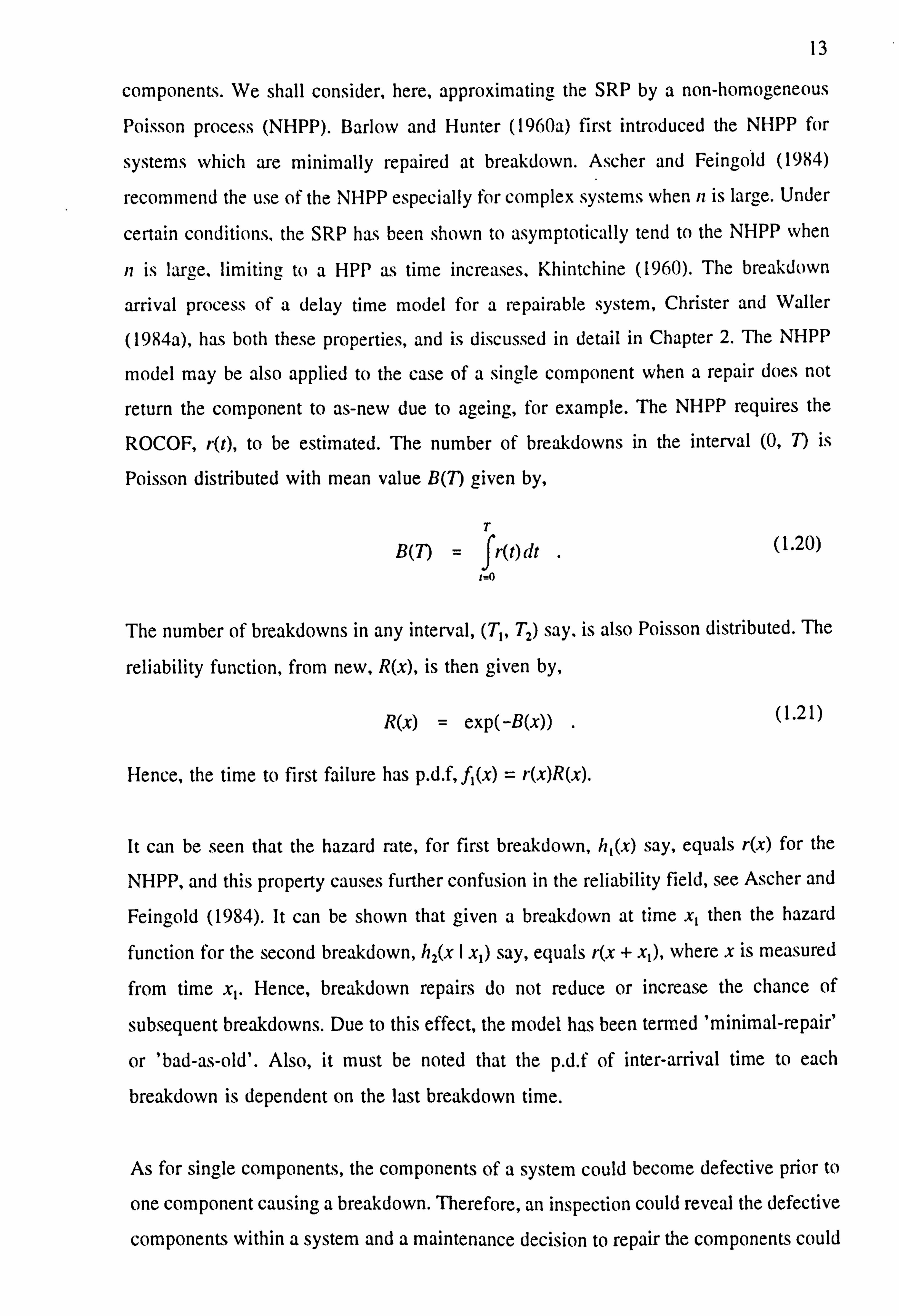
13

components. We shall consider, here, approximating the SRP by a non-homogeneous

Poisson process (NHPP). Barlow and Hunter (1960a) first introduced the NHPP for

systems which are minimally repaired at breakdown. Ascher and Feingold (19K4)

recommend the use of the NHPP especially for complex systems when ii is large. Under

certain conditions, the SRP has been shown to asymptotically tend to the NHPP when

n is large, limiting to a HPP as time increases, Khintchine (1960). The breakdown

arrival process of a delay time model for a repairable system, Christer and Waller

(1984a), has both these properties, and is discussed in detail in Chapter 2. The NHPP

model may be also applied to the case of a single component when a repair does not

return the component to as-new due to ageing, for example. The NHPP requires the

ROCOF, r(t), to be estimated. The number of breakdowns in the interval (0, T) is

Poisson distributed with mean value B(7) given by,

T

B(7) = fr(t)dt (1.20) t=0

The number of breakdowns in any interval, (T1, T2) say, is also Poisson distributed. The

reliability function, from new, R(x), is then given by,

R(x) = exp(-B(x)) . (1.21)

Hence, the time to first failure has p. d. f, f, (x) = r(x)R(x).

It can be seen that the hazard rate, for first breakdown, hl(x) say, equals r(x) for the

NHPP, and this property causes further confusion in the reliability field, see Ascher and

Feingold (1984). It can be shown that given a breakdown at time x, then the hazard

function for the second breakdown, h2(x I x, ) say, equals r(x + x1), where x is measured

from time x,. Hence, breakdown repairs do not reduce or increase the chance of

subsequent breakdowns. Due to this effect, the model has been termed 'minimal-repair'

or 'bad-as-old'. Also, it must be noted that the p. d. f of inter-arrival time to each

breakdown is dependent on the last breakdown time.

As for single components, the components of a system could become defective prior to

one component causing a breakdown. Therefore, an inspection could reveal the defective

components within a system and a maintenance decision to repair the components could

14

be applied. Hence, the number of breakdowns would be reduced through this process.

Delay time modelling for systems of this type takes into account the defective phase that

components of a system would enter over their life.

Other models for systems have included branching processes and Markov processes. For

branching processes, component dependency is modelled in that it is assumed that a

component that fails may then cause the failure of other components. For Markov

processes, a system is perceived to enter a set of defective states prior to failure, with

each time within each state having the restriction of being exponentially distributed. A

recent development has been in the introduction of a reduction factor, in that after

breakdown repair, the hazard function for the time to next breakdown is set to a level

between new and the time of the breakdown, see Kijima et al (1988).

We next consider cost and downtime models assuming a system is to be modelled by

an NHPP.

1.3.2 Models for Cost

In this section, cost models are discussed for a complex system, assuming a NHPP

model for the process of breakdown arrivals. Barlow and Hunter (1960a) consider a

form of block replacement model whereby at time T the system is completely replaced,

and breakdowns are minimally repaired over the replacement period. Assuming

instantaneous breakdown repairs, the expected cost per unit time model has identical

form in function (1.8) but with B(T) being the expected number of breakdowns assuming

an NHPP model. The model could also be applied to a system whereby at time T the

system is overhauled, repairing defective components, so that it is assumed to return to

a statistically 'as-new' system. However, the cost of overhaul would be dependent on

the number of defects within the system at time T, and thus needs to be modelled.

Chapter 2 presents a delay time model which takes this effect into account for a

complex repairable system and is based on the paper, Christer and Waller (1984a).

Other maintenance options exist, for a complex system. For example, one could replace

after N breakdowns where N is another decision option in the model, or a form of age-

15

based model whereby replacement occurs after the system operates without failure for

time T. Evidently, the model chosen would be dependent of the failure characteristics

of the system, cost levels of repair and feasibility of applying the maintenance strategy.

Practically all age-based and block replacement strategies assume the assymptotic cost

function as an objective function to optimize. Some attention has been given to

modelling an equivalent finite time horizon cost, for example, Christer (1978,1987b),

Christer and Jack (1991) and Jack (1991).

Christer and Scarf (1994) consider a replacement model for medical equipment. The

system is assumed to breakdown in accordance with a NHPP. Two decision variables

are considered, K and L. K is the number of years to replace old equipment and L is

period of use for new equipment prior to replacement. A cost model is formulated taking

into account discounting factors, over the time period K+L. There is scope to extend

the model through use of inspections. Scarf and Bouamra (1995) apply a similar model

to a set of inhomogeneous bus fleets and consider the effect of a penalty factor for

delaying replacements. Kobbacy et al (1995) assume the corrective repair process of

system is modelled by a delayed renewal process after each preventive maintenance

activity. Sensitivity analysis for the change in optimum cost policy is carried out for

varying modelling parameter values.

1.3.3 Modelling Downtime

As for single components downtime models can become complex. The two maintenance

strategies given in Section 1.2.3 could be applied to the system given identical

assumptions, except we replace the renewal assumption by the NHPP assumption.

Morumora (1970) considers a policy whereby a system is minimally repaired for

operating time T and replaced at first breakdown after operating time exceeds T. A use-

based delay time model is addressed in Chapter 2. Dagpunar and Jack (1993) consider

a policy whereby a system is minimally repaired over an elapsed time T (operating +

cumulative repair) and replaced at first breakdown after T. Christer and Waller (1984b)

present a case study of a canning line. An approximate model for downtime is proposed

whereby breakdowns are rectified over a period T and an inspection is carried to repair

16

defects at T so as to return the system to a statistically 'as-new' condition. The appendix

to the thesis outlines a delay time model to take into account the effect of stochastic

downtime.


The section details the maximum likelihood estimation technique for the NHPP

assumption of breakdown arrivals. Assume a breakdown arrival process has been

observed over an interval of time (0, T) whereby breakdowns are minimally repaired and

the system is assumed new at time 0. Let B be the number of breakdowns observed at

the ordered times, { t; } say, where t; < T, for 1Si <_ B. Cox and Hinkley (1974) derive

the likelihood as,

B

L(ý) = exp(-B(T; X))jjr(t,; X) r=1

where a, is the set of modelling parameters to be estimated and r(t; 1) and B(T; 1) are

the respective parameterised models for the ROCOF, for t>0, and the expected number

of breakdowns for time (0, T).

In testing the fit of the model, the sample cumulative failures vs. operating time could

be plotted against B(x) for 0Sx <_ T. For a numerical test, it is observed that a random

breakdown time over time interval (0,7) has the c. d. f, B(x)IB(7), given in Ross (1983).

Therefore, the empirical distribution of breakdown times over (0, T) could be compared

to the estimated c. d. f and the K-S test carried out. An additional test for the NHPP

model could also be carried out on the number of breakdowns occurring over a set of

intervals (0,7). The sample distribution can then be compared to the Poisson distribution

of mean B(T).

1.4 Delay Time Inspection Modelling

The mathematical modelling of maintenance using the technique of delay time analysis

was introduced by Professor A. H. Christer and first mentioned in the appendix to the

paper, Christer (1973). Since then, a series of papers have been written successfully

17 developing the concept and applying the model to many areas of industrial maintenance. The model arose from the observation that a component can become defective and enter

a phase prior to causing a failure such that it can be detected by an inspection and be

repaired. Evidently a component's life without any maintenance intervention, see Fig. 1.1,

can be defined as three states namely :

(1) When it is not defective (or not noticeably defective by current inspection

procedures).

(2) When it is defective, and can be inspected and repaired.

(3) When it causes a failure and needs immediate repair or replacement.

The delay time, h say, is the interval of time spent in state 2, i. e from the instant when

the component becomes defective to its necessary repair or replacement. The initiation

time, u say, is the interval of time spent in state 1, to when a defect becomes first

detectable by inspection.

Initiation Time, u Delay Time, h

01 uI tI=u+h Up time

New Defect First Breakdown Component Detectable

Fig. I. I. The initiation time and delay time of a component.

The judgement that a component is defective would be made by the maintenance

engineer. A component which is replaced whilst in the defective phase would reduce

cost and downtime compared to failure replacement. However, a compromise must be

1K

sought based on cost/downtime levels of repair and planned inspection activity. It is

evident that there is an extended scope for modelling options using the concept of delay

time.

1.4.1 Review of Papers

Christer (1982) introduces the delay time model in the context of building maintenance.

Here, a cost based system model, assuming perfect inspections, is formulated with

expected repair costs assumed to be varying over the delay time period. A method is

suggested to estimate the repair cost function by subjective estimates from engineers and

inspectors.

Christer and Waller (1984a) formally introduce the delay time model for complex

industrial systems. Models of downtime and cost are formulated assuming perfect

inspections and HPP defect arrivals. The model is then extended to NHPP defect

arrivals. The method to model imperfect inspections is then proposed. Numerical

examples are provided.

Christer and Waller (1984b) present a case study of a canning line plant. A snapshot

model is proposed to aid in locating the component types where planned maintenance

would be an effective option. The delay time p. d. f is estimated through subjective

estimates of engineers and inspectors via a questionnaire. The system model is proposed

and the predicted proportion of defects which arise as failures is modelled accurately to

the observed value for the current inspection practice.

Christer (1987a) models the reliability function of a single component subject to one

known defect type. The component is assumed to be inspected perfectly and

periodically. The model is then expanded to consider the reliability of n components in

parallel. There is scope to further expand the model to the case of imperfect inspections.

Christer (1988) develops a cost based model for the maintenance of civil engineering structures. A system model is assumed with expected repair costs varying over the delay

time period. Due to delay times being most likely to be in the order of years, the

19

probability of detecting a defect is also assumed to vary over the delay time period.

Christer and Redmond (1990) discuss a bias in the parameter estimation of the delay

time p. d. f when data collected over an operation period is censored. For example, delay

time estimates may only be obtainable at failures. The biased (or conditional) p. d. fs of

delay time are formulated for the two cases of breakdowns and inspected defects,

assuming a complex system is periodically and perfectly inspected. A maximum

likelihood estimation technique is then proposed to estimate the parameters of the true

delay time distribution. There is scope to extend the analysis to imperfect inspections

and considering the bias in the initiation time of defects. Also, the parameter estimation

bias for single components and n-component systems provides further research.

Cerone (1991) presents an approximation technique for the reliability function

formulated in Christer (1987) for a single component. Cubic splines are fitted to the

reliability function over each inspection interval. Pelligrin (1991) presents a graphical

procedure to determine the optimal inspection interval for a system delay time model

allowing for imperfect inspections.

Chillcot and Christer (1991) present a case study of applying delay time analysis to the

maintenance of coal mining equipment. A system model is assumed to predict

downtime. Due to repair downtimes being large compared to the inspection period, the

modelled process of faults arising will halt during a downtime period, and an iterative

model is proposed to take this effect into account.

Baker and Wang (1992) fit a single-component delay time model for estimating delay

time parameters by objective means given observations of times of failures and

inspection outcomes, where maintenance was carried out irregurarly. The reliability of

the components is estimated when various inspection policies are applied. This was an

important paper in extending the applicability of delay time modelling.

Christer and Redmond (1992) introduce model updating techniques when the p. d. f of delay time has been subjectively derived. The objective is to model the known

proportion of defects arising as breakdowns for the current inspection practice. The

20

actual delay time is assumed to be linearly related to the subjective estimate. The

uniqueness and existence of parameter estimates are then discussed. The scope to change

the model through assuming imperfect inspections is also addressed. An estimation

technique to estimate modelling parameters given breakdown time and defect

observations is also proposed. The case study, Christer and Waller (1984b), is used to

demonstrate the techniques proposed.

Christer and Wang (1992) present a case study of a model for condition monitoring of

a production plant. A component's wear property is modelled and a delay time model

proposed based on replacing a component when its wear reaches a certain threshold.

Baker and Christer (1994) present a review of delay time modelling. Further research

topics are outlined and a method to estimate modelling parameters from both subjective

and objetive data is proposed.

Christer et al (1995) present a case study for the maintenance modelling of a copper

production plant. A system model is assumed and the objectively based estimation of

the delay time modelling parameters undertaken using the observed times of breakdowns

and the number of defects detected at inspections. The mean downtime per breakdown

is assumed to increase prior to a planned inspection due to likely occurrence of more

severe breakdowns as the system operates. A downtime model is formulated and a

weekly planned maintenance activity is recommended.

1.4.2 Single-Component Models

We consider in this section, a delay time model for a single component. Papers and

reports on the single-component model are given by; Christer (1987), Baker (1991),

Baker and Wang (1991), Cerone (1991), Baker (1992), Baker and Wang (1992), Christer

and Wang (1992) and Baker and Christer (1994). The component is assumed to enter

a defective state prior to failure such that if detected by inspection, then repair or

replacement options exist to prevent failure. When a component is in the defective state,

it is assumed that it is still able to provide its necessary service.

21

Assume the initiation time, it, has the p. d. f and c. d. f, g(u) and G(u) say, respectively.

Likewise, the delay time, h, has p. d. f and c. d. f, f(h) and F(h) say, respectively,

independent of it. The c. d. f of time to failure, P(x) say, would then be given by the

convolution of u and h such that it +h <_ x. Therefore, P(x), is given by,

x

F(x) = J'x(u)F(x

- u) du (1.23) 11.0

and the reliability, R(x) =1- P(x).

Consider a maintenance strategy, whereby a component is replaced or repaired at failure

and only when detected in the defective phase at an inspection. Cox (1957) presents a

similar strategy based on wear level of a component at inspection We shall consider,

here, perfect inspections, and the special case that g(u) is exponentially distributed.

Therefore, an inspection would in effect be a renewal point, in that if the component is

not defective at an inspection (and consequently not replaced), then the time it to

becoming defective after inspection has the same exponential p. d. f, g(u), due to the

memoryless property. Assume the expected cost of failure replacement, planned defect

replacement and inspection have costs cf, c, and ci respectively. The objective is find the

optimum time to inspect T, after each failure-free period (0,7) of component operation.

The expected cost over each cycle, C(T), is given by,

T

C(T) =c fP(T) + (Cr +Ci) fg(u)(1

-F(T-u))du + c, (1 -GM) s

(1.24)

= (c f- Cr - ci)P(T) + c, G(T) + c, ,

after simplification. Assuming instantaneous inspection and replacement times, the

expected cycle length, M(T), is given by,

T

M(T) = JxP'(x)dx

+ TR(T) = 5R(x)dx

. (1.25)

x-o x=p

Hence, the long-term expected cost per unit time, c(T) say, is given by,

A comparison will be made, here, with the age-based policy of Section 1.2.2, whereby

a component is replaced after time T, regardless of whether it is in the defective state

22

c(T) (ý . (1.26)

or not, that is not inspecting. It will be shown by numerical example that the optimum

inspection policy can have a lower expected cost per unit time than the age-based

policy. We will assume the following values of the modelling parameters, where the

delay time distribution is also taken to be exponential:

cý = 10,

Cf = b0,

c1 = 5,

G(u) =1- exp(-0.2u) and

F(h) =I- exp(-0.3h).

It will be assumed that the cost of a planned replacement of a component at inspection,

Cr, is equal to the cost of an age-based planned replacement. The graphs of the expected

cost per unit for a range of T values are given in Fig. 1.2 for the inspection policy,

function (1.26), and the age-based policy, function (1.11). Clearly, the optimum

inspection policy results in lower expected cost per unit time. The optimum inspection

time is shorter than the age-based replacement time. This is to be expected, as

inspections will reduce the frequency of failures and component replacements.

I

F U

ci t E

C

U

a Q) 8

xx w

1

1.5

11

0.5-

10-

9.5-

9-

8.5-

8-

7.5-

7 12 3 4 5 6 7 9

Inspection Policy --. -

Age-Based Policy

Decision Parameter, T

Fig. 1.2. Comparison of an inspection policy and age-based replacement.

23

1.4.3 System Models

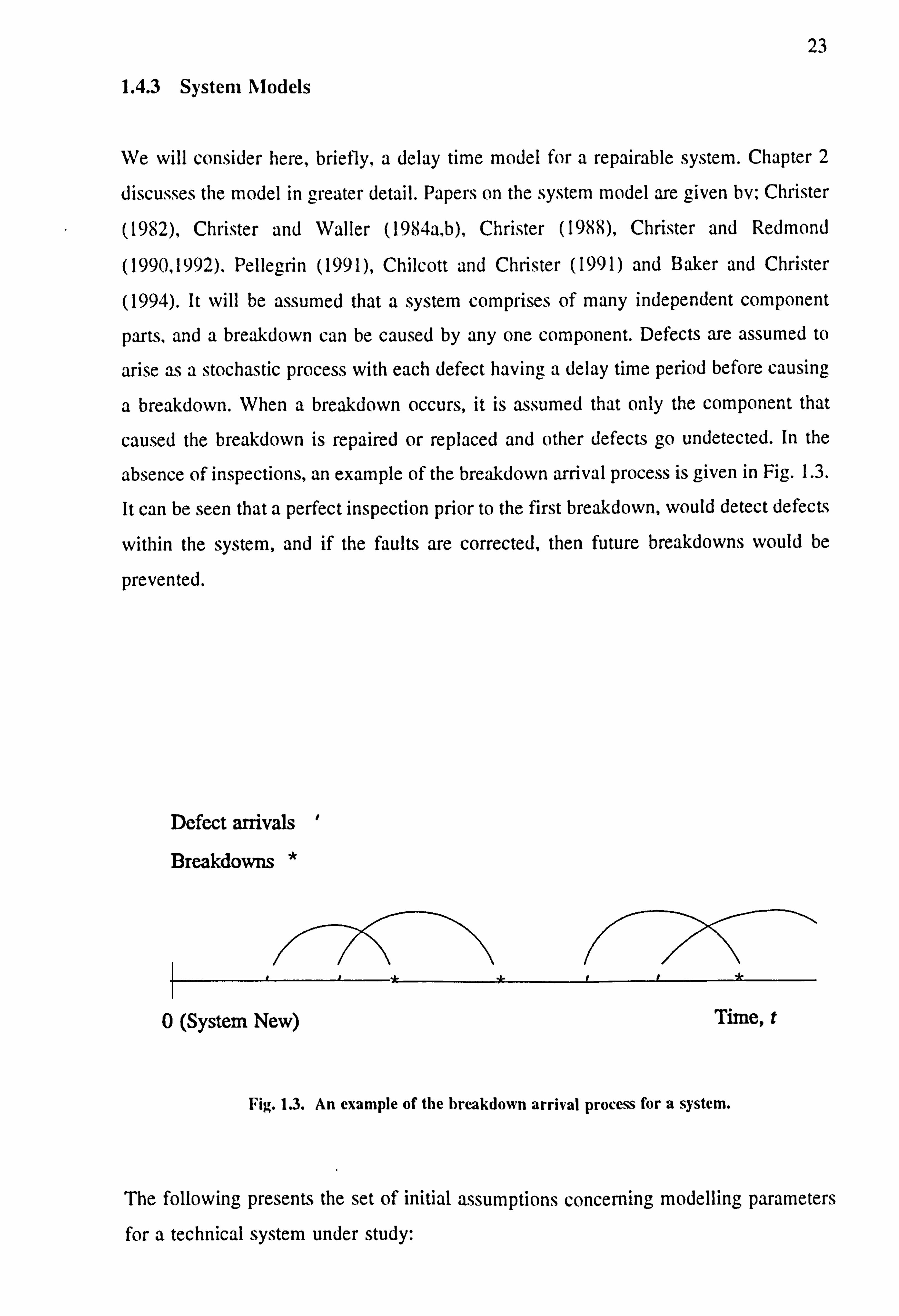
We will consider here, briefly, a delay time model for a repairable system. Chapter 2

discusses the model in greater detail. Papers on the system model are given bv, Christer

(1982), Christer and Waller (1984a, b), Christer (1988), Christer and Redmond

(1990,1992). Pellegrin (1991), Chilcott and Christer (1991) and Baker and Christer

(1994). It will be assumed that a system comprises of many independent component

parts, and a breakdown can be caused by any one component. Defects are assumed to

arise as a stochastic process with each defect having a delay time period before causing

a breakdown. When a breakdown occurs, it is assumed that only the component that

caused the breakdown is repaired or replaced and other defects go undetected. In the

absence of inspections, an example of the breakdown arrival process is given in Fig. 1.3.

It can be seen that a perfect inspection prior to the first breakdown, would detect defects

within the system, and if the faults are corrected, then future breakdowns would be

prevented.

Defect arrivals '

Breakdowns *

0 (System New) Time, t

Fig. 1.3. An example of the breakdown arrival process for a system.

The following presents the set of initial assumptions concerning modelling parameters for a technical system under study:

24

(a) At time 0, the system is in a new or 'as new' state, that is defect free.

(b) Defects arise within the system, independently, as a homogenous Poisson

process (HPP) with rate parameter k, over time.

(c) Delay times, h. are independent of arrival time it and are described

by the probability density function (p. d. f), f(h) say. with finite mean p.

(d) Those defects which cause breakdowns over time are repaired with

negligible time at failure.

(e) A breakdown has a repair cost, which is independent of the defect arrival

time, the delay time and the repair time. The repair cost is assumed to

have a mean cb.

(f) Inspections are perfect.

(g) There is a constant time T between successive inspections.

(h) The expected cost of an inspection is c1.

(j) An inspection takes time, d1, to undertake, and all defective components

that may be found are repaired/replaced within this time.

(i) The expected cost of a repair to a defective component at an

inspection is cd.

It will be shown in Chapter 2, that the process of breakdown arrivals of the system described above, under failure-based maintenance (FBM), is a non-homogeneous Poisson

process (NHPP). A characteristic function of the inspection policy is the proportion of defects which would arise as breakdowns, b(T) say. This has been derived by Christer

and Waller (1984a), and is given by,

T

b(7) =Tf (T - h) f(h) dh (1.27) h-0

The model for expected cost per unit time, c(T) say, is then given by,

`(ý = kTb(T)cb + kT(1-b(T))cd + c1 (1.28)

T+d, ,

over each cycle, (0, T+ d).

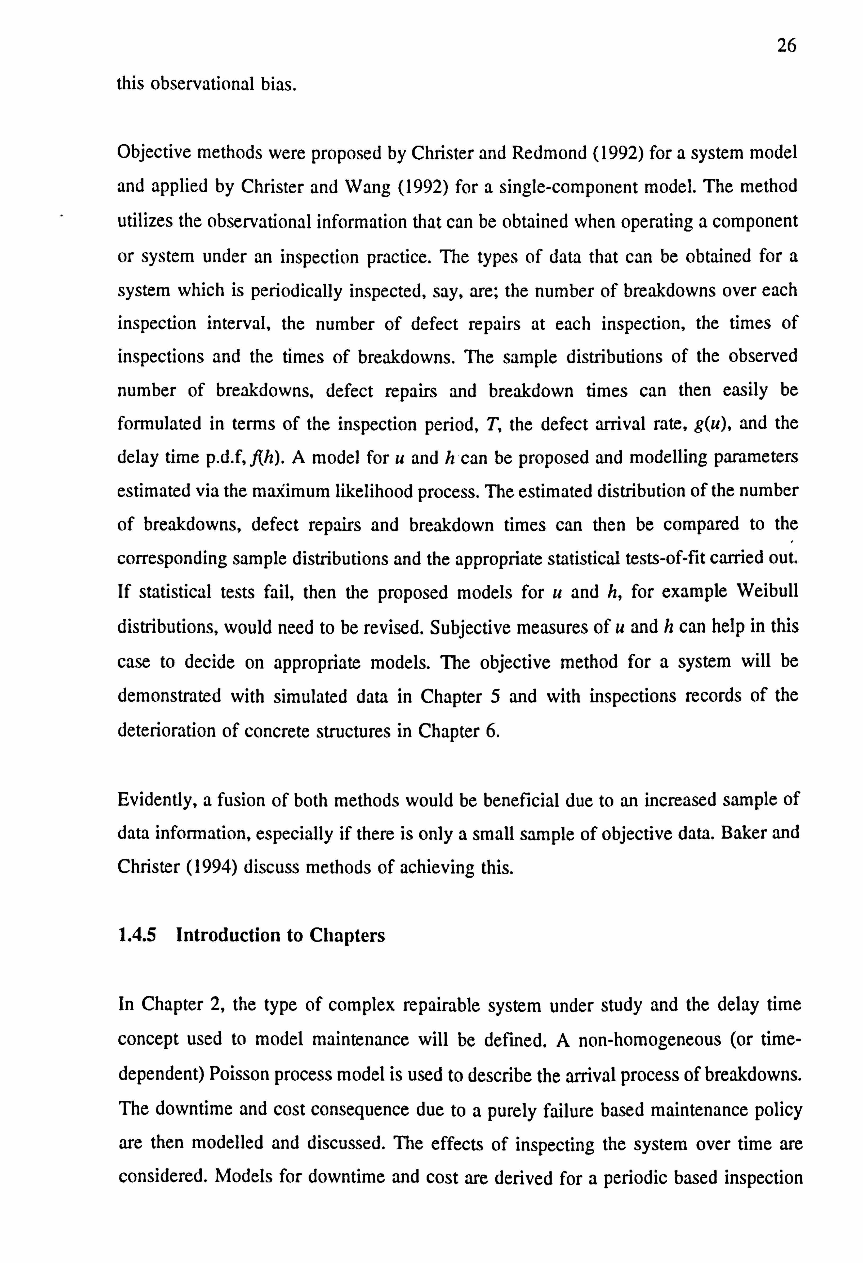
To model downtime, assume db is the expected downtime of a breakdown repair, and

25

that db is small compared to T. Hence, the approximate expected downtime per unit

time, d(T) say, over each cycle (0, T+ dj), is given by,

d(ý = db kTb(T) + dt

T d1 (1.29)

+

The delay time model can further be applied to imperfect inspections, non-homogeneous

rates of defect arrivals and to other inspection-type policies. These model developments

and others will be discussed in Chapter 2.


Central to the application of delay time analysis, is the accurate estimation and testing

of modelling parameters concerning the selected initiation time and delay time model

of components and systems. There have been essentially two approaches to the problem,

that is the subjective method and the objective method.

The subjective method was introduced in the context of building maintenance, Christer

and Waller (1984b). Questionnaires were compiled and presented to engineers and inspectors. The questions were aimed at obtaining subjective estimates of the initiation

time and delay time of specific parts. At a breakdown, the engineer was asked how long

ago the defect would have arisen. Thus, yielding a point estimate of both the initiation

and delay time. At an inspection, an estimate is also required on how much longer a defective component could be delayed before it would cause a breakdown, in order to

obtain an estimate of its delay time. Standard estimation and test-of-fit procedures can

then be carried out to estimate the distribution (for single-components) or rate process (for systems) of the initiation time, u, and the delay time p. d. f, f(h). However, a model formulated from only subjective data, would not necessarily model observational

characteristics of the known inspection practice, such as the observed proportion of defects arising as breakdowns and the sample properties of the observed breakdown

times. Hence, a form of revision or updating is necessary after subjective estimation. Chapter 3 presents methods for a system model to update and test estimated modelling

parameters. Chapter 4 presents the case when subjective data is further censored, by

considering the situations when a subjective data set can only be obtained at breakdowns

or, perhaps, only at inspections. A maximum likelihood technique is proposed to remove

26

this observational bias.

Objective methods were proposed by Christer and Redmond (1992) for a system model

and applied by Christer and Wang (1992) for a single-component model. The method

utilizes the observational information that can be obtained when operating a component

or system under an inspection practice. The types of data that can be obtained for a

system which is periodically inspected, say, are; the number of breakdowns over each

inspection interval, the number of defect repairs at each inspection, the times of

inspections and the times of breakdowns. The sample distributions of the observed

number of breakdowns, defect repairs and breakdown times can then easily be

formulated in terms of the inspection period, T, the defect arrival rate, g(u), and the

delay time p. d. f, f(h). A model for u and h 'can be proposed and modelling parameters

estimated via the maximum likelihood process. The estimated distribution of the number

of breakdowns, defect repairs and breakdown times can then be compared to the

corresponding sample distributions and the appropriate statistical tests-of-fit carried out. If statistical tests fail, then the proposed models for u and h, for example Weibull

distributions, would need to be revised. Subjective measures of u and h can help in this

case to decide on appropriate models. The objective method for a system will be

demonstrated with simulated data in Chapter 5 and with inspections records of the

deterioration of concrete structures in Chapter 6.

Evidently, a fusion of both methods would be beneficial due to an increased sample of data information, especially if there is only a small sample of objective data. Baker and

Christer (1994) discuss methods of achieving this.

1.4.5 Introduction to Chapters

In Chapter 2, the type of complex repairable system under study and the delay time

concept used to model maintenance will be defined. A non-homogeneous (or time-

dependent) Poisson process model is used to describe the arrival process of breakdowns.

The downtime and cost consequence due to a purely failure based maintenance policy

are then modelled and discussed. The effects of inspecting the system over time are

considered. Models for downtime and cost are derived for a periodic based inspection

27

policy. Initially, inspection will be assumed perfect and this requirement is then relaxed

to include the case of imperfect inspections. Extensions to these models will be

developed and conditions involving modelling parameters are derived for the decision

to optimize cost or downtime by an inspection based policy. Numerical examples will

be provided. An alternative inspection policy based on inspecting a system after a

specific period of use (or operation) will also be discussed. The chapter is based on the

paper, Christer and Waller (1984a).

In Chapter 3, procedures are constructed for estimating the parameters necessary to

formulate the models derived in Chapter 2. These will be constructed and based upon

the experience gained and the data collected in operating repairable systems over time.

Two types of data will be focused on, namely subjective and objective. Subjective data

can arise from engineers' estimation of the delay time of specific defects at breakdowns

and inspections. Thus, data of this type is expected to be in error. However, the

collection of this data has been shown to be possible and prior delay time distributions

have been estimated in specific cases, see Christer and Waller (1984b), Chilcott and

Christer (1992), Christer and Desa (1992). The objective data for estimating the delay

time distribution is based upon observations of times of breakdowns and defect

detections. This data will aid the estimation of delay time parameters and the testing of

the fit of the subsequent maintenance model. A maintenance model formulated with a

substantial subjective input to delay time parameter estimates could not guarantee to

automatically model the "status quo" characteristics of the system. That is subjective

data may not imply that which is currently observable. Management interest may be in

cost, downtime or proportion of defects which arise as failures under a current

inspection practice. Eitherway, updating procedures are given to force the subjectively

based model to agree with "status quo" observation. The situation is demonstrated in

Fig. 1.4, where b(7) is the prior model for the probability a defect arises as a breakdown

and b,, * is the observed estimate of this probability for the inspection practice, To. This

updating procedure could be considered as a "model tuning process". We will find in

Chapter 3 that there is not necessarily a unique option for updating. However, a

selection criteria is given based on other information, which may be available, over the

system data collection period. The chapter is substantially based on the paper, Christer

and Redmond (1992).

28

In Chapter 4, the case of having a censored data sample with which to estimate a delay

time distribution is discussed. As previously outlined, one situation which could arise

is that delay times and initiation times of defects may only be readily estimated from

either breakdown events or when defects are detected at inspections. Another situation

could be a non-balanced mixture of these two extremes in that we may not be able to

obtain an estimate of delay time and initiation time for each defect which has arisen

over a survey period. In the case of censored data, a bias in the estimated distribution

of delay times or initiation time would exist. This will be established by deriving the

respective conditional p. d. f of delay time and initiation time associated with defects

which arise as breakdowns, and those which are detected at inspection. The p. d. fs will

be derived for both perfect and imperfect inspection policies. An example of the

unconditional p. d. f and conditional p. d. fs of delay time is given in Fig. 1.5, assuming

a delay time distribution f(h), defect arrival rate k and inspection period T= 10. A

maximum likelihood estimation technique and appropriate tests of model fit are then

recommended to cope with the observational bias introduced. Much of the work of this

chapter is based on the paper, Christer and Redmond (1990).

In Chapter 5, a simulation study is undertaken to further investigate and verify the delay

time models and proposed method of analysis. Simulation programs, written in Pascal,

have been used to simulate the delay time process given sets of input parameters and

assumptions. Methods of simulation are shown for the case of perfect inspections and

instantaneous repair of breakdowns. Then, these assumptions are relaxed to imperfect

inspection and non-instantaneous breakdown repairs. The output of simulation

experiments are analyzed and compared to the appropriate theoretical values of the

models of the earlier chapters. An investigation is undertaken into the accuracy and

effectiveness of the parameter estimation procedures given in Chapters 3 and 4.

Correction of bias is carried out on censored simulation data. The effects of not

correcting for bias but using an updating method, as a further option, is also explored.

Fig. 1.6 demonstrates the situation when correction of bias has not been undertaken

compared with the theoretical model and an observed value for the proportion of defects

arising as breakdowns. An iteration method is developed which alternates between

updating the scale parameter of a Weibull delay time distribution and only estimating

29

the shape parameter using maximum likelihood. The estimation of delay time

distribution parameters based upon only observational data (failure times and number

of defects detected at inspections) is also demonstrated. Results are shown for simulated data sets and conclusions drawn.

In Chapter 6, an account is given on research supported by the Science and Engineering

Research Council (grant: GR/F 61196) over a three year period. The project was in

collaboration with members of the Civil Engineering Department at Queen Mary and

Westfield College, London University. The main objectives were to collect and publish

data on the observed rates of deterioration of particular defect types in a large number

of concrete bridges and to develop predictive mathematical models that relate inspection

frequency to maintenance costs. The delay time model is expanded to an extra phase in

order to model the deterioration process of cracking and spalling in concrete, see Fig.

1.7. Costs of repairs are then expected to increase over the cracking and spalling phases.

Due to the inspection records of components, only intervals containing the times to the

states are available. A model for the distributions of times within each phase is proposed

and estimation, via maximum likelihood, is undertaken, given the censored observations.

Appropriate tests of model fit are carried out using the Kaplan-Meier estimate of the

reliability function. Single component and multi-component cost models are then

formulated for a variety of inspection and maintenance options. The motivation for the

project was in part associated with the prototype modelling paper for inspection practices

of major concrete structures, Christer (1988). A paper is to be published on this research

project in the European Journal of Operational Research in 1996.

30

The probability a defect causes a breakdown, b(7)

4

b(1?

Fig. 1.4. The prior model, b(7), compared to the known current practice.

ci

Unconditional

Breakdowns

Inspection repairs

Fig. 1.5. The unconditional and conditional p. d. fs of delay time.

0 TO Inspection Period, T

U2468 10 12 14 16 Delay Time

31

9

cd 2

^L LL

True Model --+- Inspection Prior -- Breakdown Prior

Fig. 1.6. The effects of not correcting for bias of conditional delay time sets.

Defect free Phase Cracking Phase Spalling Phase

IIIi 0u u+h u+h+v Defect Multiple Minor Severe Free (New) Cracks Spalling Spalling

Fig. 1.7. The deterioration phases of a concrete component.

05 10 15 20 25 30 Inspection Period, T

32

1.5 Discussion

This chapter has presented an overview of past and current developments in maintenance

modelling. It is evident that delay time models and other new models are now

increasingly being applied and tested through case studies. However, there is evidence

of a deficiency of models for maintenance that takes into account the physical process,

be it chemical, electrical or mechanical, that leads to a component failure. Geraerds

(1972) regards the selection of statistical models for component and system failure

behaviour as a subsection of a complex maintenance model of an organisation, that also

takes into account such factors as maintenance planning and control, designs of systems,

inventory problems and the feedback of results. Dekker et al (1995) consider also the

planning of the maintenance activities for a group of components with different

estimated optimal policies. It is shown that combining the maintenance activities, by

delaying or bringing forward planned maintenance for some components with increased

cost penalty, can reduce overall maintenance costs. This is due to the setup cost being

shared. Hence, the necessary fusion between mathematical models and organizational

planning and constraints are evolving in the maintenance field.

Over the past ten years, delay time modelling has undergone considerable development

and is increasingly being accepted as an important concept for the real world modelling

of maintenance of components and systems. There have been models which have

touched on the concept, for example, Cox (1957, p. 121) introduced a wear model such

that a component can be defect free or enter a defective state prior to failure. This is

equivalent to having a finite probability of zero delay time. An inspection model is

presented to take into account this effect. Cozzoloni (1968) formulates a model whereby

a system is assumed to have an unknown number of defects after a planned maintenance

activity with each defect having a delay to cause failure. It is shown that the process of

breakdowns will be a non-homogeneous Poisson process, as with the delay time system

model. Butler (1979) classifies a component as functioning, functioning but defective,

and failed. An inspection is also assumed to possibly increase the chance of failure due

to the chance of observing a component in the defective state. However, a Markov

model is formulated, thereby restricting the distribution of u and h to exponential. Lewis

(1972) suggests an accumulation model whereby defective components which are

33

detectable and do not cause failures, i. e having infinite delay time, are repaired at a

failure. The expected repair time is then correlated with operating time. Jansen and Van

der Duyn Schouten (1995) present a model for maintenance optimization of parallel

production units. In the discussion of extensions to this model, it is assumed that the

lifetime distribution of a component may be modelled by a convolution of two non-

identical exponential distributions. The unit is described as 'good' in the first phase and

'doubtful' in the second phase. The condition can be tested and a decision can then be

made on whether to overhaul. Hence, the model allows an extra decision option through

the use of inspections. In addition, the maintenance cost could be further optimized

when it is decided to take only the doubtful (or defective) units out of production for

overhaul.

Statistical methods, testing and policy formulations are evidently being developed and

formalised for the delay time model with the growing experience through applications.

It is important that statistical tests are carried out in confirming all postulated

assumptions, e. g the renewal assumption of a perfect inspection. A method to identify

the optimal and feasible policy type (e. g periodic or age-based inspections) for a

component or system also needs to be addressed. The following chapters of the thesis

develop the theory of the delay time model, formalise statistical methods for revising,

estimating and testing modelling parameters and apply the model to the deterioration of

concrete structures.

35

Chapter 2

Delay Time Models for Maintenance of a Repairable System

2.1 Introduction

In this chapter, the type of repairable system under study and the delay time concept

used to model maintenance will be defined. A non-homogeneous (or time-dependent)

Poisson process model is used to describe the arrival process of breakdowns. The

downtime and cost consequence due to a purely failure based maintenance policy are

then modelled and discussed.

The effects of inspecting the system over time are considered. Models for downtime and

cost are derived for a periodic based inspection policy. Initially, inspection will be

assumed perfect and this requirement is then relaxed to include the case of imperfect

inspections. Extensions to these models will be developed. Conditions involving the

modelling parameters are derived for the existence and uniqueness of an optimal

inspection based policy. Numerical examples will be provided. An alternative inspection

policy based on inspecting a system after a specific period of use (or operation) will also

be discussed.

Finally, conclusions are dawn and suggestions are given for further areas of research.

2.2 Delay Time Concept for a Repairable System

The repairable system under study can be a simple or complex electrical or mechanical

plant where the objective is to model the cost or downtime consequences for various

maintenance policies available to the engineer. The following assumptions are assumed

36

to characterise the system being modelled:

(a) The system is modelled as a two state system where, over its service life, it can

be eith°r operating acceptably or down for necessary repair or planned

maintenance.

(b) The system is comprised of many component parts or sections which are prone

to become defective independently of each other when the system is operating.

(c) Defects which may have arisen in the system, deteriorate over an operating time.

The deterioration may be due to operating conditions, such as vibration or

environmental effects. However, the system can remain functioning in an

acceptable manner until breakdown.

(d) The breakdown will be assumed to have been caused by one of the defects which

has deteriorated sufficiently to affect the operating performance of the system as

a whole (essentially a series type configuration of independent component parts. )

Failure is assumed evident to the user and corrective maintenance is essential.

Hence, the system would then cease operating due to the failed component. Once

the failed component has been replaced or restored to a 'statistically new'

condition, the system is assumed to be able to return to the operating state.

However, other defective components can still be present if only corrective repair

of the failed component is carried out.

The concept used to model the system described is delay time analysis, conceived by

Christer (1973) and introduced into the context of building maintenance by Christer

(1982) and then to industrial maintenance by Christer and Waller (1984b). A defective

component is assumed to become defective at a point in time, u say, when the system

is operating such that it is detectable by current inspection procedures. This epoch will

be called the initiation time for the defect and a similar process applies to all other

defects. The arrival process of defects in the system will be a superposition of u values

across all the components. Due to a large number of component parts in the system, the

superposition of defect arrivals in the system, u, will be assumed to be approximated by

37

a Poisson process in the homogeneous (HPP) or non-homogeneous (NHPP) form,

unaffected by breakdown repairs over time.

Initiation Time, u Delay Time, h

0u

LU+h

Up time

New Defect First Breakdown Component Detectable

Fig. 2.1. The initiation time and delay time of a defect.

The delay time, h, of a defective component is the interval of operating time from the

initiation time, it, to the point at which the defective component will cause a breakdown

(or failure), at time t -= it + h, see Fig. 2. I. Over the delay time period (u, u+ h), it is

possible that the defective component in question can be repaired or replaced at a

planned inspection thus preventing breakdown and consequences associated with it. The

delay time of a component will be assumed random and independent of the initiation

time. In general, components which are non-identical or not subjected to similar

operating conditions would have delay times which are not identically distributed.

However, it will be assumed that each random defect arrival, at time it, in the

superposition process of defect arrivals across all components, will have a delay time,

h, acceptably modelled as being identically distributed and independent of it.

The above assumptions are characteristic of those which have been successfully used in

modelling inspection policies for building and industrial maintenance, see Christer and

Waller (1982,1984b), Chilcott and Christer (1991), Christer and Wang (1992), Baker

and Nang (1992,1993), Christer and Wang (1)95), Christer et al (1995).

38

2.3 Type of Maintenance Activities

We, here, introduce the various types of maintenance activities that can be carried out

on the system. Gits (1986) defines a set of maintenance activity options to be considered in the design stage of a maintenance concept. Three main types will be investigated

a) Breakdown repair, a procedure to repair only the defective component which

caused failure.

b) Inspection, an observation process or intervention where defects could be located

and consequently repaired thus preventing breakdowns (if repairs are perfect).

Inspection is then classed as a preventive maintenance activity.

c) Overhaul or replacement, a maintenance process where the whole system is

assumed to return to a statistically 'as new' condition.

Inspections or overhauls are planned and can be carried out at planned points in time

(e. g periodically), or could be initiated at breakdowns (ist or 2nd etc. ) The type of

policy for a particular system in question would depend on the failure characteristics of

the system, such as defect rate and delay time distribution, for example, as well as the

objectives of maintenance. We shall see, for example, that as may be expected, the

quality of inspections and the cost and downtime levels of inspections and breakdown

repairs contribute to determining the appropriate maintenance policy.

2.4 Failure Based Maintenance (FBM)

The models formulated in this section describe the process of occurrence of breakdowns

and so provide a conceptual framework for when inspection models are considered. Our

task is to derive models of repair, downtime and cost over time when performing

corrective repair to components which cause breakdowns. It is assumed that breakdowns

are dealt with by only repairing the defective component, that is FBM. The situation is

demonstrated in Fig. 2.2, where it is assumed, at first, that breakdowns are instantaneously repaired. The following presents the set of initial assumptions concerning

modelling parameters for the first technical system under study, and are based upon the

previous section:

39

(a) At time 0, the system is in a new or 'as new' state, that is defect free.

(b) Defects arise within the system, independently, as a homogenous Poisson

process (HPP) with rate parameter k, over time.

(c) Delay times, h, are independent of arrival time it and are described

by the probability density function (p. d. f), f(h) say, with finite mean p.

(d) Those defects which cause breakdowns over time are repaired with

negligible time at failure.

(e) A breakdown has a repair cost, which is independent of the defect arrival

time, the delay time and the repair time. The repair cost is assumed to

have a mean cb.

It is also convenient, here, to define F(h) as the cumulative distribution function (c. d. f)

of delay time h.

Defect arrivals '

Breakdowns *

0 (System New) Time, t

Fig. 2.2. An example of the breakdown arrival process.

2.4.1 Number of Breakdowns arising over Time

If we define t to be a time scale in units of time since the system was in the new or 'as

new' state, then breakdowns would arise as a stochastic point process along the t axis.

The failure arrival pattern is a superposition of failure arrivals across all the components

40

within the system. It is clear that over an indefinite period of time and in the absence

of inspection based maintenance, each defect can be expected to cause a breakdown

event.

The process of breakdown arrivals can be described by defining, B, say, to be the

cumulative number of breakdowns after operating the system for time t and define

B(t) = E(B), the expected number of breakdowns in (0, t). To derive, B(t), we observe

that a defect arising in an interval (u, it + du), for u<t, where du is small, will cause

a breakdown in interval (0, t) if its delay time h<t, it, see again Fig. 2.1. The

probability that h<t-u is F(t - u). Clearly, the expected number of defects to arrive

in (u, u+ du) is kdu, due to HPP defect arrivals. Hence the expected number of

breakdowns caused by defects arriving in (u, it + du) is,

F(t - u)kdu . (2.1)

The expected number of breakdowns, B(t), can then be obtained by integrating over all

possible it < t. Hence,

rr

B(t) =kf F(t - u) du =kf F(h) dh (2.2) u=0 h-0

which is given in Christer and Waller (1984a). As expected, B(t) is a monotonically

increasing function, with its differential being kF(t) when F(t) is differentiable.

Considering the integrand as a product of I and F(h), the expression for B(t) can be

integrated by parts and re-written,

B(t) =k tF(t) -

r fhfth)A

, h=0

(2.3)

which can be seen to tend to the line k(t - µ) as t tends to infinity, where µ is the mean

delay time. This suggests that a property of the model is that breakdown occurrences

arise asymptotically as a HPP when defects arrivals arise as a HPP independently of the

delay time distribution. It may be necessary and intuitive to obtain the distribution of B,. An analogy of the stochastic process, B1, arises in queuing theory. The process is an

example of an M/G/oo queue, see Ross (1983) or Medhi (1983, p. 321). In this situation

customers arrive according to. a Poisson process and each one is immediately served

41

with a commonly distributed service time. Customers are analogous to defect arrivals

and the service time is analogous to the delay time. A breakdown is analogous to a

completed service for a customer. Ross (1983) shows that the arrival process of

completed services is a non-homogeneous Poisson process (NHPP), see also Parzen

(1962, p. 125). Hence, Bt is Poisson distributed with mean B(t), i. e,

p{Br = n} = B(t)ne-acn

n! (2.4)

Hence, for example, the reliability of the system can be determined, that is C"I", the

probability no failures arise in interval (0, t). The NHPP requires a time-dependent rate

function, say r(t), such that r(t)dt represents the expected number of breakdowns in

interval (t, t+ dt). The function r(t) has been called arrival intensity, see Parzen

(1962, p. 125), or rate of occurrence of failures (ROCOF), see Ascher and Feingold

(1984, p. 4). For this process, r(t) is given directly by equation (2.2) as,

r(t) =B '(t) = kF(t) ,

(2.5)

which can be seen to be a multiple k of the delay time c. d. f. As t -4 oo, we have from

equation (2.5) that the rate of arrival of breakdowns tends to the defect arrival rate, k.

Hence for this system the breakdown process tends asymptotically to an HPP, identical

to the process of defect arrivals, that is the system performance would tend to a limit.

It follows that in the limit the inter-arrival time between breakdowns would tend to the

exponential distribution of mean 1/k, which will prove to be an important property in

asymptotic considerations of cost and downtime. Properties of the inter-arrival times of

breakdowns for a general NHPP, can be found in Parzen (1962, p. 138).

2.4.2 Modelling Cost

The repair cost of a breakdown can include factors such as manpower, materials, lost

production and environmental damage. Independence is assumed between the number

of breakdowns occurring in time t and the cost of each repair, with an a°sumed mean

cost per repair of Cb. Letting, c,, say, be the repair cost of the n'th failure, then the

cumulative repair cost, say C, is given by,

42

B' (2.6) B cn for Bt >_ 1 Cr =

n=1 0 for B1 =0

which is a cumulative Poisson process when the repair costs, c, are independent and

identically distributed, see Cox (1957). Defining C(t) as the total expected cost after

operating the system for time t we have,

C(t) = E(C) = cbB(t) , (2.7)

which is given in Christer and Waller (1984a), though derived slightly differently there.

The expected asymptotic repair cost per unit time over all time, c� say, is then given by,

c� = lim Cýtý = kcb

t--_ t (2.8)

This is an expected result, since k defects are expected to arrive in unit time, each with

an expected subsequent repair cost, cb, incurred when the defect ultimately causes a

breakdown.

0 2.4.3 Modelling Downtime

Here we relax assumption (d) so that repair times are finite and our interest is in

modelling the effects of downtime. It will be assumed that each breakdown is repaired

with a repair time independent of each other, and with an identically distributed repair

time with mean, db say. The situation is depicted in Fig. 2.3. When the system is in the

down state, it will be assumed that new defects do not arise within a breakdown repair

time and that other defects are effectively frozen, that is deterioration (i. e the expiry of delay time) does not take place for other defects which may be present in the system at

the time of failure. When db is small, the repair downtime can be thought of as being

a repair cost, that is cost is measured in units of downtime. Hence, the expected

cumulative downtime over real time t can be approximated by; D(t) say, given by,

D(t) = dbB(t) ,

(2.9)

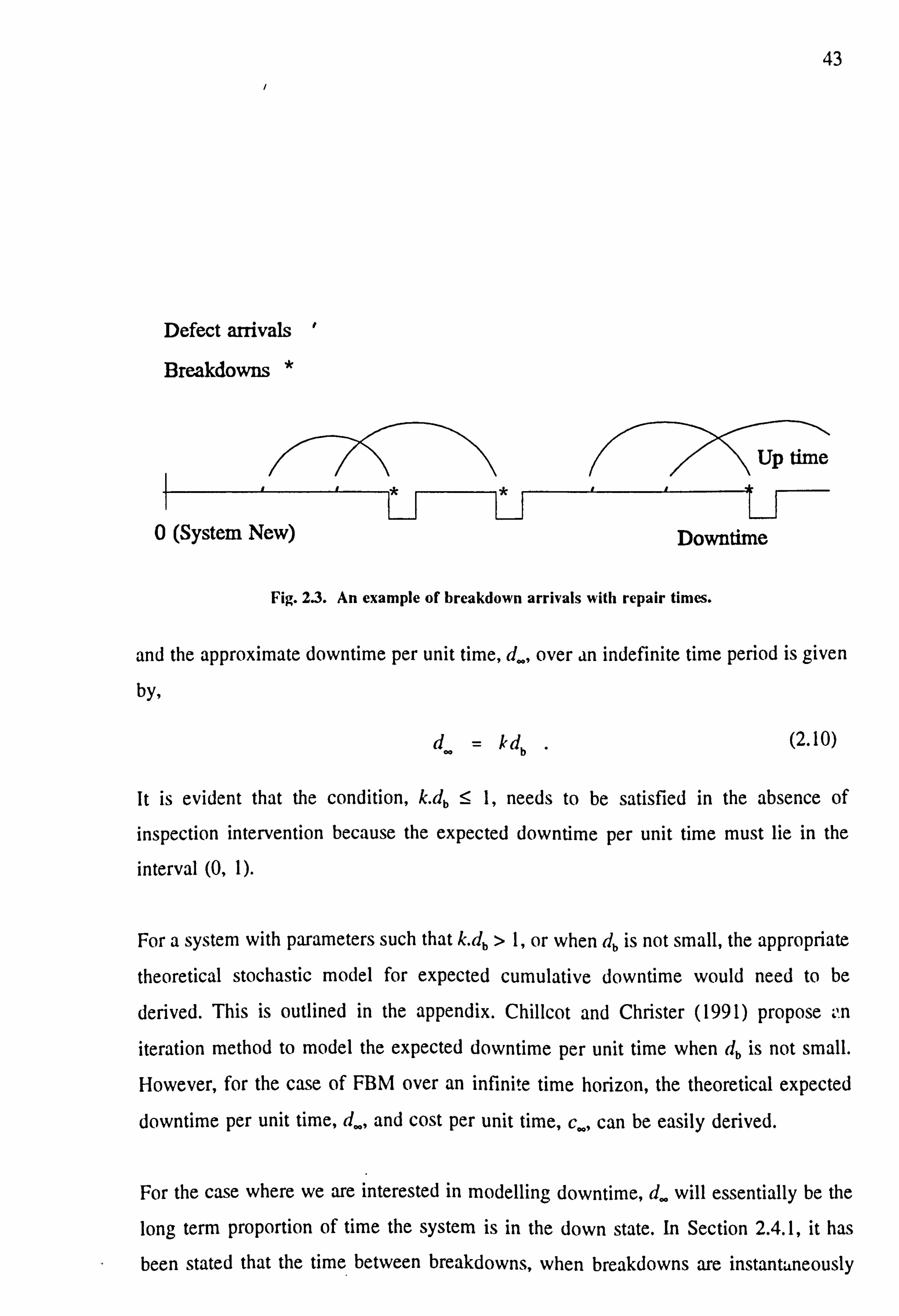
43

Defect arrivals '

Breakdowns *

Up time *

0 (System New) Downtime

Fig. 2.3. An example of breakdown arrivals with repair times.

and the approximate downtime per unit time, d., over an indefinite time period is given

by,

d� = kdb . (2.10)

It is evident that the condition, k. db <_ 1, needs to be satisfied in the absence of inspection intervention because the expected downtime per unit time must lie in the

interval (0,1).

For a system with parameters such that k. db> 1, or when db is not small, the appropriate

theoretical stochastic model for expected cumulative downtime would need to be

derived. This is outlined in the appendix. Chillcot and Christer (1991) propose ý. n

iteration method to model the expected downtime per unit time when db is not small.

However, for the case of FBM over an infinite time horizon, the theoretical expected

downtime per unit time, d,,, and cost per unit time, c,,, can be easily derived.

For the case where we are interested in modelling downtime, d� will essentially be the

long term proportion of time the system is in the down state. In Section 2.4.1, it has

been stated that the time between breakdowns, when breakdowns are instantaneously

44

repaired, tend to the exponential distribution, mean 1/k. When a period of downtime

occurs, the stochastic process of breakdown arrivals effectively stops for the duration.

Hence, the operating time between breakdowns would tend to the exponential

distribution in the long term. We assume here that repair times are independent and

identically distributed, with mean db. Hence in the long term, the FBM process can be

thought of as being an alternating renewal process of up and downtimes, see Cox

(1957, p. 8O). The long term proportion of time spent in the down state, d,,, is then given

by,

d= E(downtime) kdb (2.11) 1 +kdb E(uptime) + E(downtime)

which, as required, lies in the interval (0,1) for any positive values of k and db. The

result is also given in Smith (1985, p. 27) for systems which have exponential time

between failure and arbitrary downtime distribution. It is worth noting that d� is

independent of the delay time distribution or parameters from it. However, the speed at

which the limit is achieved will depend upon the delay time distribution form. Also, it

can be seen that the approximate model needs the condition that kdb is small compared

to unity.

In the long term, performing FBM, the up-down cycle length, that is the uptime before

repair plus downtime of repair, has the expected value 1/k + db. An expected cost, cb,

would be incurred over this interval. Therefore, the theoretical asymptotic cost per unit

time, c., can be derived by considering the process as a renewal reward process. The

value c� is then the ratio of expected cost for one repair, cb, to the expected cycle length

Ilk + 'b, giving,

kc c� =b (2.12)

1+ kdb

2.4.4 Non-Homogeneous Defect Arrivals

We can extend the model to a more general technical system where defects may arrive

as a NHPP, with properties given in Section 1.3.1. The NHPP requires a rate function

g(u) such that g(u)du represents the expected number of defects arriving in the small

45

interval (it, it + du), when the system has been operating for time it, see Christer and

Waller (1984a), Christer and Wang (1995). Hence, following the analysis in Section 2.3,

the expected number of breakdowns, B(t), will take on the convoluted form,

I

B(t) =f g(u) F(t -u) du 14 =0

(2.13)

given in Christer and Waller (1984a). The occurrence of failures, once again, will be

NHPP due to the underlying process of defect arrivals and the independence between

delay times and defect arrivals, see Ross (1983). The ROCOF is given by,

I

r(t) =B '(t) = fg(x)f(t

- x)dx (2.14)

x=o

The number of breakdowns, B1, to arrive in operating time t, is Poisson distributed, with

mean B(t), due to breakdown arrivals arising as an NHPP. The models for cumulative

expected downtime and cost, derived in the chapter, will have identical forms for NHPP

defect arrivals, but using the revised B(t), given above. However, the asymptotic

behaviour of breakdown occurrences and consequent downtime and cost per unit time,

will depend on the defect arrival rate g(u) and delay time p. d. f }(h).

Many of the breakdown maintenance models presented above, or their variants will be

used in the subsequent sections and chapters on inspection modelling. These models are

not management models in the sense that they have no decision variable to control the

failure pattern of the system. What the models do provide is estimates and forecasts of

the stochastic consequence of a particular practice, which has value to management. It

has been shown that modelling the failure characteristics of a repairable system can be

achieved using the technique of delay time. Our objective, next, is to model the

consequences of the inspection option, that is build a management model.

2.5 Periodic Based Inspection (PBI)

In this section, it is proposed to construct models assuming a policy of inspection on a

46

periodical basis. The models will aim to predict cost and downtime consequences for

alternative inspection periods. Inspection will at first be considered perfect and then

relaxed to include the case of imperfect inspections.

A perfect inspection is a planned maintenance stoppage of the system whereby all

defective components present in the system are located and corrected to a statistically

'as new' condition within the time allocated for inspection. The time constraint is

imposed initially for simplifying convenience and will later be relaxed. It will be

assumed that a perfect inspection returns the entire system to a 'statistically-as-new'

condition, i. e it is analogous to a renewal, replacement or overhaul. An inspection is also

assumed not to generate any defects. The following additional assumptions to the FBM

set will be applied, see Christer and Waller (1984a):

(a) There is a constant time T between successive inspections irrespective of

the cumulative breakdown repair time within each inspection interval (i. e

T will not always be the operating time between inspections).

(b) Breakdowns impose a small amount of downtime compared to the

inspection period T, with expected value db, db « T.

(c) The downtime required for each inspection is a constant d1.

(d) The expected cost of an inspection is c1.

(e) The expected cost of a repair to a defective component at an inspection is cd (< cb, the expected cost of a breakdown).

(f) If the system is down for breakdown repair, and is due for inspection, the

component which has caused the breakdown has the repair completed

within the time allocated for inspection, di.

The effect of inspection is shown by example in Fig. 2.4, where it is evident that perfect

inspections reduce the number of breakdowns. However, over frequent inspections will

incur an increased downtime and cost penalty. Hence, a compromise needs to be sought

to identify the most appropriate inspection interval. The assumptions of the model were

influenced by the research at a canning line plant, Christer and Waller (1984b), whereby

daily inspections were planned, breakdowns were repaired within the inspection period

and defective components were rectified at inspections. Management adopted the

predicted optimum policy which was interestingly close to the current inspection

practce.

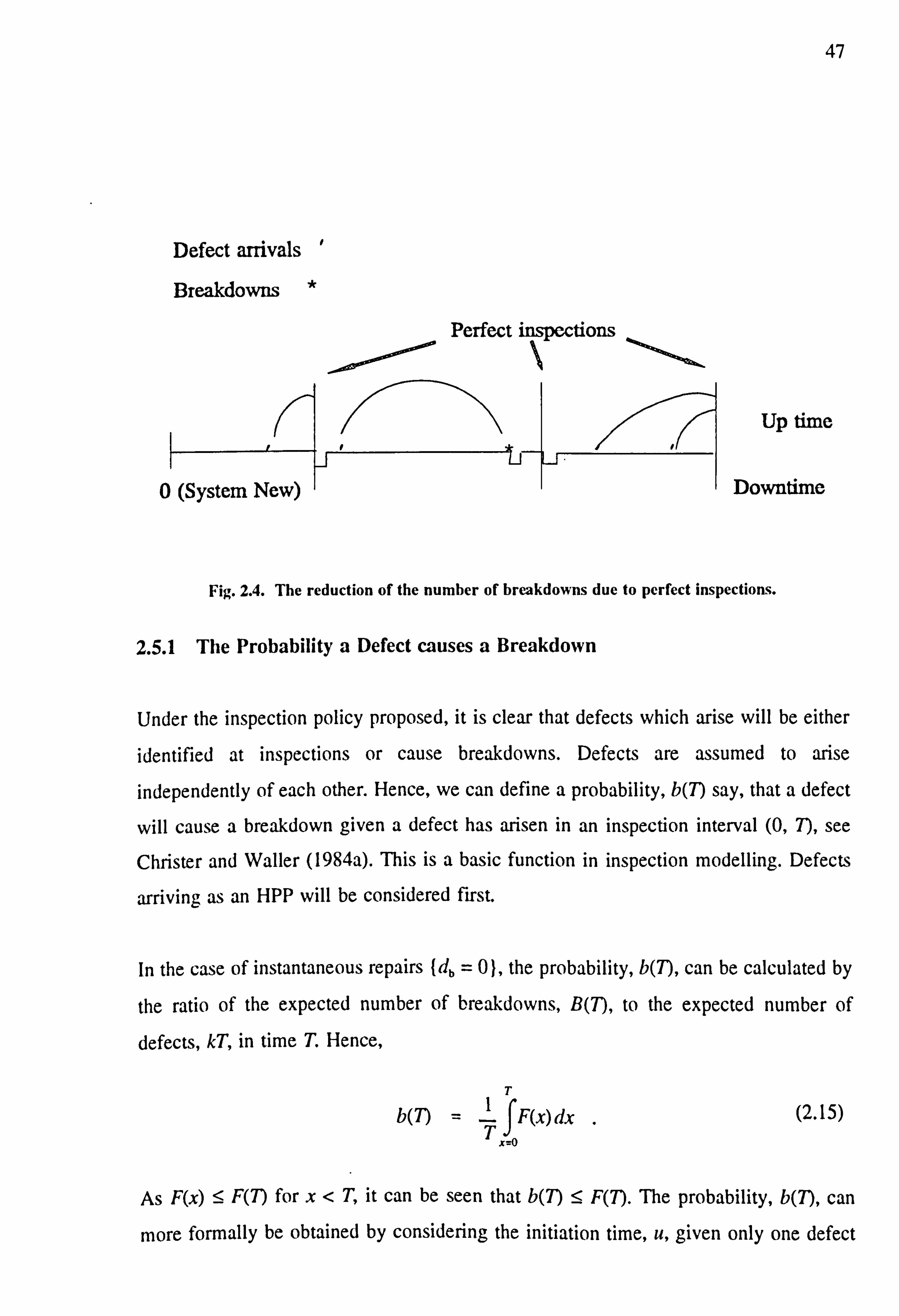
47

Defect arrivals '

Breakdowns *

Perfect inspections

ýý Up time

0 (System New) ý Li r-I

Downtime

Fig. 2.4. The reduction of the number of breakdowns due to perfect inspections.

2.5.1 The Probability a Defect causes a Breakdown

Under the inspection policy proposed, it is clear that defects which arise will be either

identified at inspections or cause breakdowns. Defects are assumed to arise

independently of each other. Hence, we can define a probability, b(T) say, that a defect

will cause a breakdown given a defect has arisen in an inspection interval (0,7), see

Christer and Waller (1984a). This is a basic function in inspection modelling. Defects

arriving as an HPP will be considered first.

In the case of instantaneous repairs {db = 0}, the probability, b(7), can be calculated by

the ratio of the expected number of breakdowns, B(7), to the expected number of

defects, kT, in time T. Hence,

T

b(T) IF(x)dx .

(2.15) x=0

As F(x) <_ F(T) for x<T, it can be seen that b(T) S F(T). The probability, b(T), can

more formally be obtained by considering the initiation time, u, given only one defect

4 has arisen in (0, T). The distribution of it will be uniform over interval (0,7), due to

HPP defect arrivals. If the defect has a delay time in the small interval (h, h+ (1h), an

event occurring with probability f(h)dh, then it would cause a breakdown if the

initiation time satisfies it <T-h, which has probability (T - h)/T. Hence, combining

these probabilities and summing over all possible it, we have,

T

b(7) _ 1(T

- h)f(h)dh (2.16) h=0

which was originally formulated in Christer and Waller (1984a). The functions (2.15)

and (2.16) provide approximations for the probability a defect leads to a breakdown,

when db >0 and db « T, and can be shown to be equivalent by integrating equation

(2.16) by parts. The function is an approximation due to the stochastic accumulation of

breakdown repair time over each interval (0,7). The characteristic shape of the function

b(T) is shown in Fig. 2.5. It can be seen to increase from zero, monotonically, to 1 when

T tends to infinity, as expected. Due to F(0) =0 and b(T) _<

F(T), then b(7) -4 0 when

T -4 0. Essentially, the T=0 implies that defects are immediately detected when arisen

and subsequently repaired, which implies no failure occurrences and so b(0) = 0. The

policy of FBM described in Section 2.4 is equivalent to T= oo. The differential of b(T)

is given by,

T

b'(7) _Lf {F-(T) - F(x)) dx X--o

which is non-negative, implying the function is non-decreasing.

2.5.2 Modelling Downtime

The total expected downtime incurred over time interval (0, T) can be approximated by

the function (2.9), if assumption (b) holds, namely db « T, and the expected number of

breakdowns B(T) is small. These conditions are required due to the random loss of

operating time over each inspection interval. Due to inspections being perfect and the

cycle length constant at T+ d1, we have that the approximate expected downtime per

unit, d(T), over each cycle (0, T+ d), is given by,

49

Probability a defect leads to a breakdown, b(7)

1

Fig. 2.5. The probability, b(T), a defect arises as a breakdown.

d(T) = D(T) + di dbB(T) + (11 kTdbb(T) + dI

(2.18) T+d1 T+d1 T+d1

which was originally formulated in Christer and Waller (1984a). The asymptotic value

of function (2.18), as T -4 oo, can be seen to be kdb since b(T) tends to unity. In

comparing this value with the limit for the actual asymptotic downtime per unit time

(2.11), it can be seen that an additional condition for this model to be asymptotically

valid is that kdb should be small so that the value k. d)(1 + k. db) is close to kdb. If the

condition is not satisfied then the optimal inspection period may be in error and either

the stochastic model of downtime, given in the appendix, or the downtime model for an

alternative inspection policy (Section 2.6) would need to be derived.

The value of T which minimizes the objective function (2.18) can be found graphically,

or by numerical search or when analytically valid by differentiating with respect to the

decision variable T and setting the result to zero to obtain the equation,

T

di F(T) + fhfth)dh

- d'

=0 (2.19)

h=o kdb

0 Inspection Period, T

50

The differential of the L. H. S of equation (2.19) is (T + (I1)f(T), which is positive for

T>0 and f(T) > 0. Hence, it follows that the L. H. S is a monotonically increasing

function. Thus, a finite solution r, if it exists, will be unique if f(T) > 0.

Inspection will not always be an optimal choice and a finite solution to equation (2.19)

will not always arise since its existence is dependent on the selected parameters. The

function on the L. H. S of equation (2.19) is negative at T=0. Hence, for a solution, T",

to this equation, a necessary and sufficient condition for a unique solution is that the

L. H. S must be positive as T --- oo. It then follows that for a finite solution to equation

(2.19) to exist the following condition must hold,

Il+ dI 1- 1>0 (2.20) kdb

If this condition is not satisfied by the estimated parameters, then FBM or another form

of planned maintenance scheme will provide the lowest expected downtime per unit time

for the system in question. When considering PBI, d(T) would be a monotonically

decreasing function with a limit of k. db as T -) °°. If condition (2.20) is satisfied then

the solution inspection interval, 7', obtained from equation (2.19) is the recommendation

for optimizing downtime assuming a policy of inspection on a regular periodical basis.

2.5.3 Modelling Cost

We now turn our attention to the task of modelling cost under the assumptions given in

Section 2.5. In order to model costs either cumulative or on an expected time basis, we

need to calculate the expected number of defects which can be located and repaired at

each inspection. Denote AT as being the number of defect arrivals in (0,7) and ST as the

number of defects in the system, which have arisen but not yet caused a breakdown, and

therefore identified by perfect inspection at time T. Also let BT be the number of

breakdowns in each inspection interval. Therefore, as each defect would either be in the

system or have caused a breakdown,

AT=B,. + ST E(AT) = E(BT) + E(ST) (2.21)

Due to HPP defect arrivals, the expected number of defects to arrive in time T,

51

E(AT) = U. Thus the mean number of defects in the system at time T since last

inspection, S(7) = E(ST) say, is given by,

S(T) = kT - B(T) = kT(1 - b(n) =k f(1

- F(x))dx

. rte

(2.22)

which, using expression (2.3), tends to the product of the defect arrival rate and the

delay time mean, kµ, as T increases, . This is analogous to the immigration-death

population model (or MIM/- queue) where k is the immigration rate and 1/µ is the death

rate, see Cox and Miller (1965, p. 168). The limit, kµ, is the expected size of the

population (in this case defects) as T increases to infinity. The limit is also the expected

number of defects to be found on first inspection when switching from a contingency

breakdown policy, i. e FBM, to a perfect inspection policy, shown in Christer (1982).

Medhi (1982, p. 321) shows that in the related queuing situation, ST is Poisson distributed

with mean given by equation (2.22) when breakdown repair times are negligible. Ross

(1983) shows that ST and B,. are independent. These properties will aid in model

parameter estimating and testing the fit of the model.

The expected total cost for breakdowns, C(T) = cbB(T), would here apply over each

inspection cycle, T+ d1. The expected cost of repairs carried out at inspections is cdS(T)

where as before S(T) is the expected number of defects detected at T. It is assumed that

the cost of an inspection is c,. Hence, if we define c(T) to be the expected cost per unit

time over each cycle, (0, T+ d), then for the case of effectively instantaneous repairs,

C(T) = T+d1 (2.23)

Clearly, the model c(T), (2.23), would serve as an approximation for the case of non-

instantaneous repairs, provided assumptions (b) and (f) hold, namely db> 0 and db « T.

The approximation improves as the approximate downtime of breakdown repairs per unit

time over interval (0,7), namely dbB(T)/T, decreases.

The asymptotic value of function (2.23), that is kcb, can be found in the FBM case by

ý[ + CbB(`) + CdS(T)

noting that B(T)IT tends to k and S(T)IT tends to 0, as T -4 °°. In order to investigate

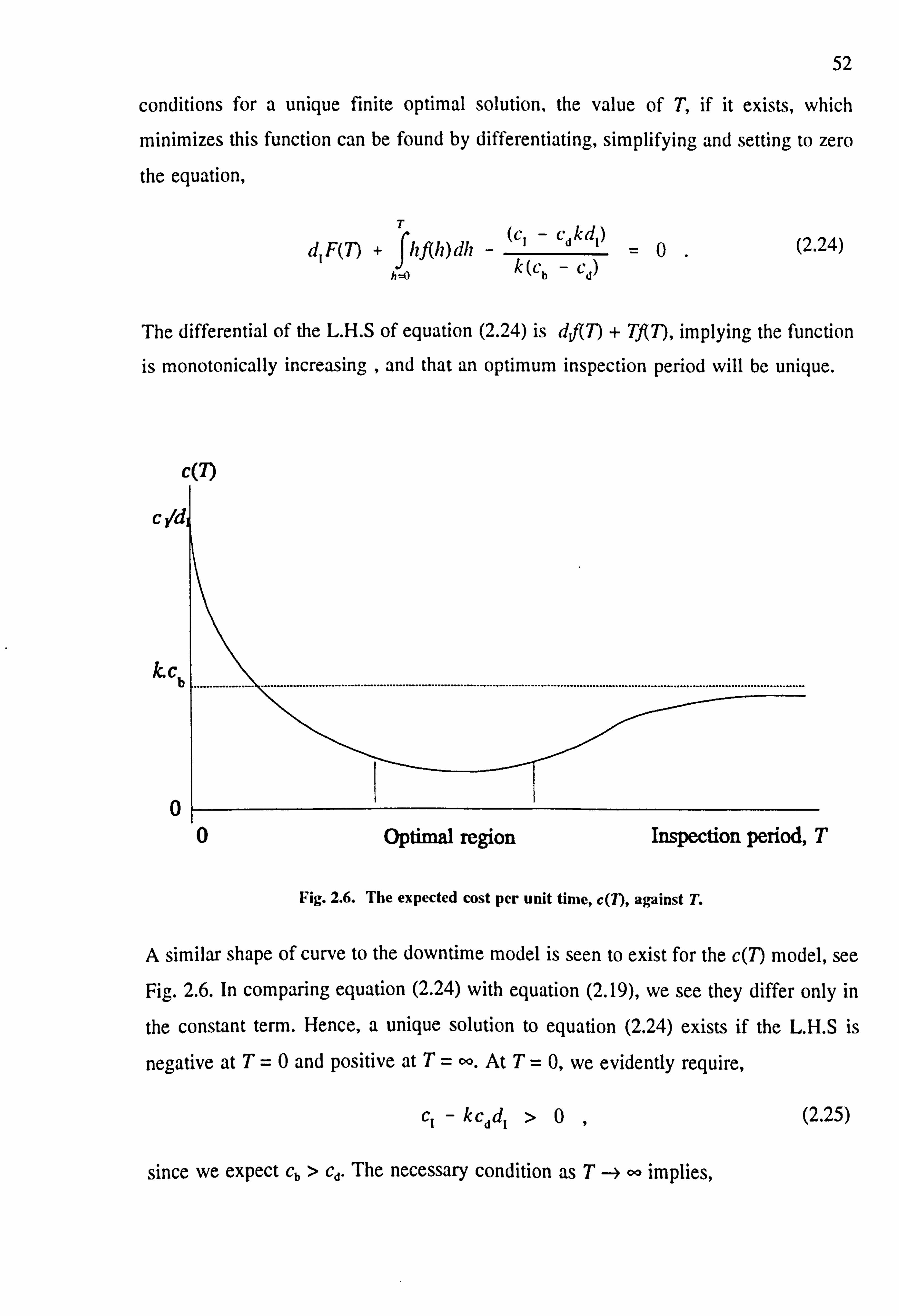
52

conditions for a unique finite optimal solution, the value of T, if it exists, which

minimizes this function can be found by differentiating, simplifying and setting to zero

the equation,

T

d1F(T) + Jhf(h)dh

- (c1 - cdkdi)

=0. (2.24)

ham) k(cb Cd)

The differential of the L. H. S of equation (2.24) is d j(7) + Tf T), implying the function

is monotonically increasing , and that an optimum inspection period will be unique.

C(T)

c Id

IGCb

0

Fig. 2.6. The expected cost per unit time, c(7), against T.

A similar shape of curve to the downtime model is seen to exist for the c(T) model, see Fig. 2.6. In comparing equation (2.24) with equation (2.19), we see they differ only in

the constant term. Hence, a unique solution to equation (2.24) exists if the L. H. S is

negative at T=0 and positive at T= °°. At T=0, we evidently require,

cI - kcA >0, (2.25)

since we expect cb > Cd. The necessary condition as T --* co implies,

0 Optimal region Inspection period, T

53

+ (ci - kcddi)

>0 (2.26) k(cb - Cd)

2.5.4 Perfect Inspection Models with Non-Homogeneous Defect Arrivals

Here, we now relax the HPP assumption of constant rate defect arrivals and let g(u) be

the instantaneous rate of defect arrivals at time it from the 'as new' condition. The

defects are assumed arise in time as a non-homogeneous Poisson process (NHPP).

Therefore the total expected number, K(7) say, of defects to arrive in interval (0,7) is

given by,

T

K(T) = fg(u)du

u-0

(2.27)

The arrival time, u, assumed for a random defect, given to arise over interval (0,7) has

the p. d. f, q(u; T) say, given by,

- g(II) 9(u; T) = K(ý

for 0<u<T, (2.28)

which is a relationship shown by Ascher and Feingold (1984, p. 32), and given in

Christer and Redmond (1990). Essentially, if, B say, failures have been observed in time

interval (0, T), then the B ordered breakdown arrival times, y1, y2, ..., YB say, are the

order statistics of a sample, size B, taken from the p. d. f (2.28).

In this case, the probability that a defect arises as a failure now takes on the form,

T

b(7) = 5q(u; F(T - u) dcc

U --o

T

= 5Q(T-h; T)ith)dh

A=0

(2.29)

where Q(u; T) = K(u)/K(T) is the c. d. f of u. The form of the models for downtime and

cost have identical structures (2.18) and (2.23) respectively, but now having

B(T)=K(T)b(7) and S(7) = K(7) - B(7) = K(7)(1 - b(T)), given in Christer and Waller

(1984a). Due to Q(u; 7) :51, it can be seen that b(7)., 5 F(T) for the case of NHPP defect

arrivals as well as HPP defect arrivals. It is noted that in the special case of HPP when

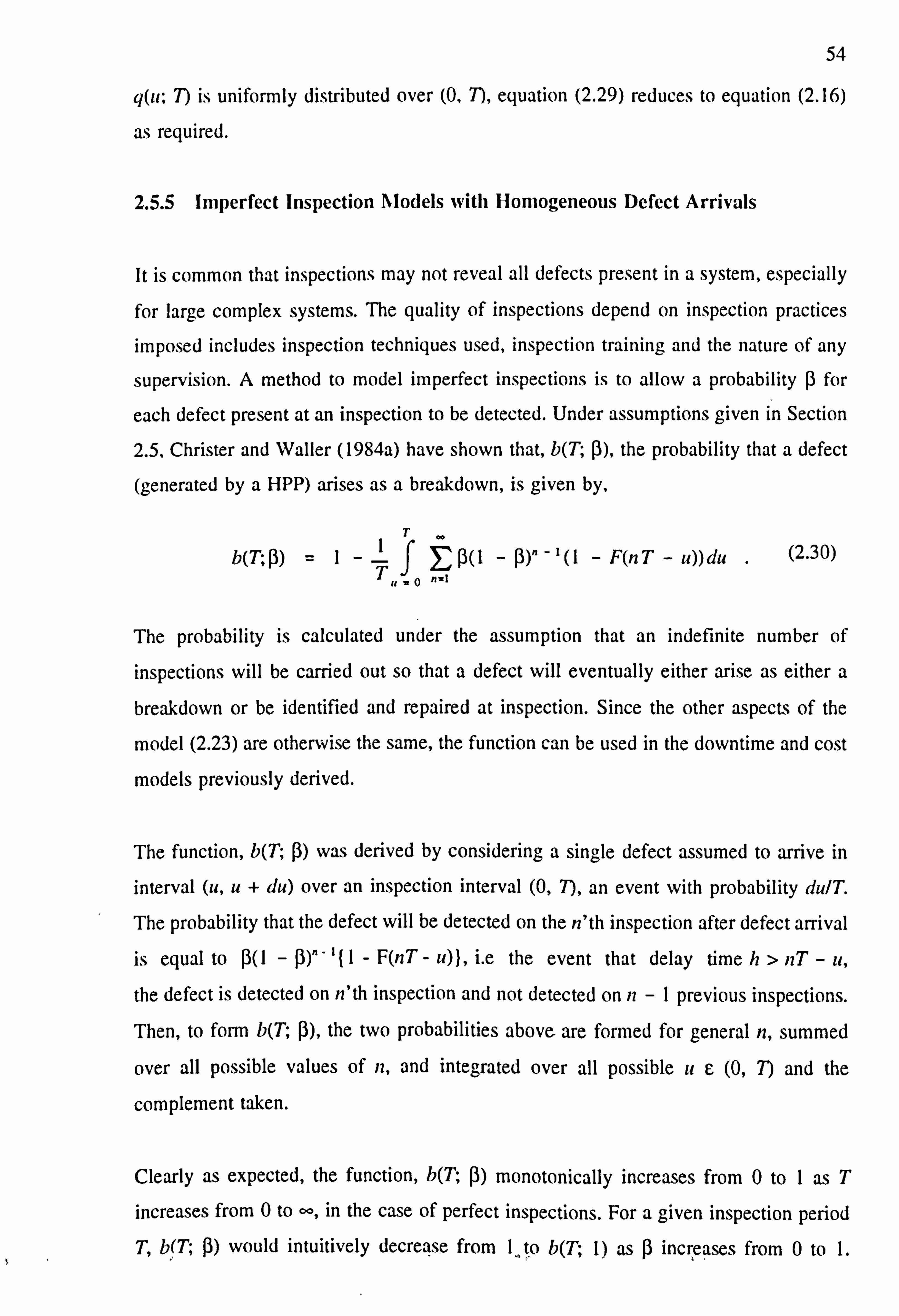
54

y(u, T) is uniformly distributed over (0, T), equation (2.29) reduces to equation (2.16)

as required.

2.5.5 Imperfect Inspection Models with Homogeneous Defect Arrivals

It is common that inspections may not reveal all defects present in a system, especially

for large complex systems. The quality of inspections depend on inspection practices imposed includes inspection techniques used, inspection training and the nature of any

supervision. A method to model imperfect inspections is to allow a probability ß for

each defect present at an inspection to be detected. Under assumptions given in Section

2.5, Christer and Waller (1984a) have shown that, b(T; (3), the probability that a defect

(generated by a HPP) arises as a breakdown, is given by,

T eO

b(T; (3) =1-! f (3(1

u=0 nI - (3)" -1(1 - F(n T- u)) du .

(2.30)

The probability is calculated under the assumption that an indefinite number of

inspections will be carried out so that a defect will eventually either arise as either a

breakdown or be identified and repaired at inspection. Since the other aspects of the

model (2.23) are otherwise the same, the function can be used in the downtime and cost

models previously derived.

The function, b(T; ß) was derived by considering a single defect assumed to arrive in

interval (u, u+ du) over an inspection interval (0,7), an event with probability du/T.

The probability that the defect will be detected on the n'th inspection after defect arrival

is equal to ß(1 - ß)" " II 1- F(nT - u)), i. e the event that delay time h> nT - it,

the defect is detected on n'th inspection and not detected on n-1 previous inspections.

Then, to form b(T; ß), the two probabilities above are formed for general n, summed

over all possible values of n, and integrated over all possible ue (0, T) and the

complement taken.

Clearly as expected, the function, b(T; 1) monotonically increases from 0 to 1 as T

increases from 0 to °°, in the case of perfect inspections. For a given inspection period T, b(T; ß) would intuitively decrease from I

., to b(T; 1) as 1 increases from 0 to 1. 1I ,

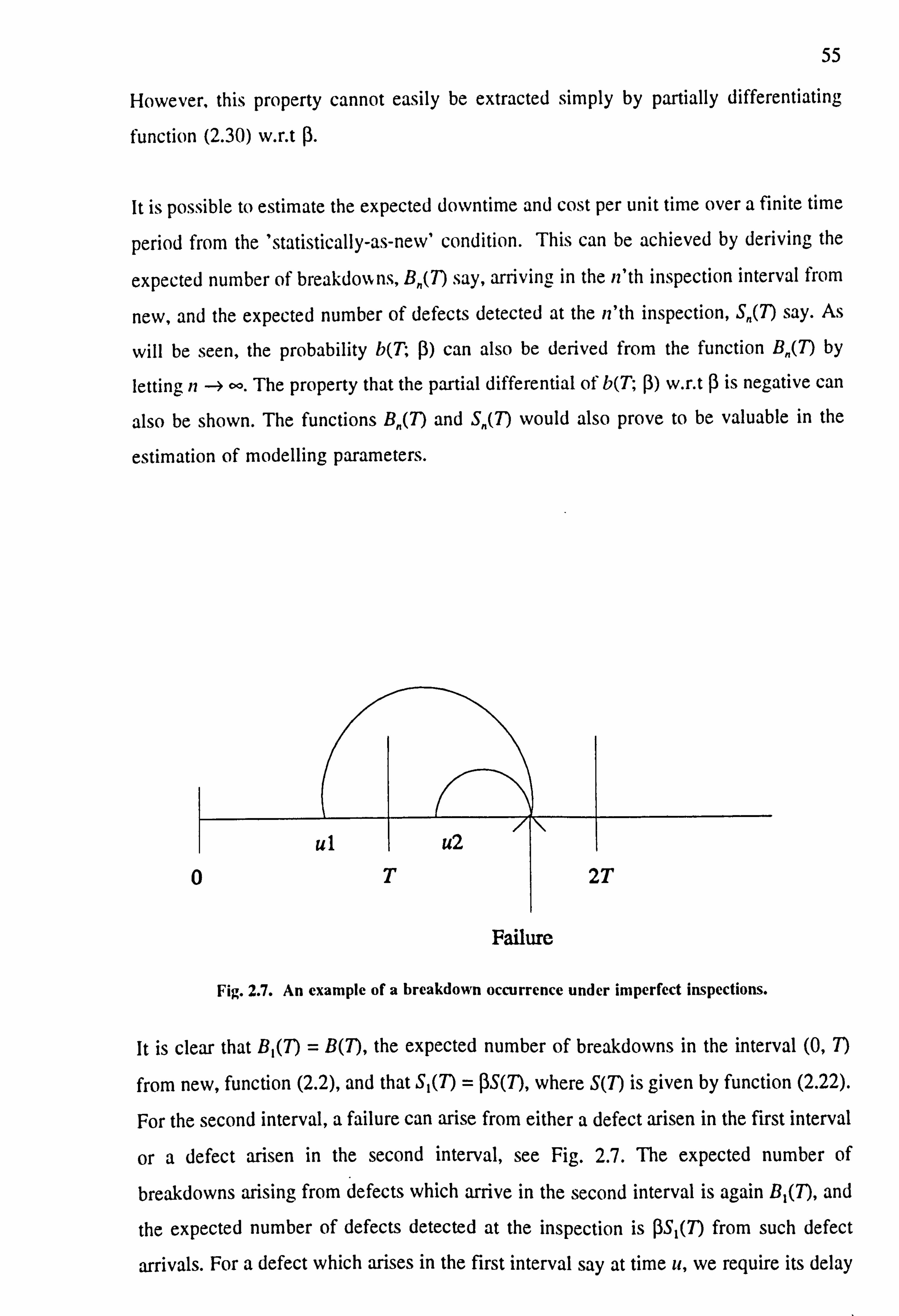
55

However, this property cannot easily be extracted simply by partially differentiating

function (2.30) w. r. t P.

It is possible to estimate the expected downtime and cost per unit time over a finite time

period from the 'statistically-as-new' condition. This can be achieved by deriving the

expected number of breakdo%k ns, B, (T) say, arriving in the n'th inspection interval from

new, and the expected number of defects detected at the n'th inspection, Sn(T) say. As

will be seen, the probability b(T; (3) can also be derived from the function BS(T) by

letting n -- oo. The property that the partial differential of b(T; ß) w. r. t (3 is negative can

also be shown. The functions B�(T) and SS(T) would also prove to be valuable in the

estimation of modelling parameters.

C

Failure

Fig. 2.7. An example of a breakdown occurrence under imperfect inspections.

It is clear that B, (T) = B(T), the expected number of breakdowns in the interval (0,7)

from new, function (2.2), and that S, (7) _ 13S(7 ), where S(T) is given by function (2.22).

For the second interval, a failure can arise from either a defect arisen in the first interval

or a defect arisen in the second interval, see Fig. 2.7. The expected number of

breakdowns arising from defects which arrive in the second interval is again B1(7), and

the expected number of defects detected at the inspection is PS1(7) from such defect

arrivals. For a defect which arises in the first interval say at time it, we require its delay

56

9

time, h, in interval (T - it, 2T - u) and to be not detected at T, in order to cause a

breakdown in the second inspection interval (T. 27). The probability of this event is

(t - ß) { F(2T - u) - F(T - u) } and the expected number of defect arrivals in (u, it + du)

is kdu. Therefore integrating the combined probability for all it <T and adding B(T) for

the expected number of breakdowns arising from defect arrivals in the second interval,

it follows that, using expression (2.2) for B(T). B, (T) is `ºiven by.

T

B2(T) = B(T) + k(l -ß) 5F(2T-u)_F(T-u)ilti

I, _0 (2.31)

2T

=k (1 - (3)ý-ý fF(IT

'=ý «=o - u) - F((i -l )T - u)}du ,

where F(h) =0 for h<0. To formulate B�(T), the expected number of defects

breakdowns arriving in the n'th inspection interval due to defects arisen in the interval

(0, nT), we notice that the expected number of breakdowns in the n'th interval attributed

to defects arriving in inspection intervals other than the first is B�_, (T). Therefore, for

a defect arising in the first interval at time it we require its delay time, h, to be interval

(nT - it, [n -l IT - u) and not to be detected at n-1 inspections to cause a failure in

the n'th inspection interval. Using previous analysis, it follows that B�(T) is given by,

T

B(7) = B�-1(T) + k(1-(3)"-' J(nT-u) -F((n -1 )T-u)}du

�-o

nT

= kE (1-ß)'-I f (F(iT-ui)-F((i-1)T-u))dci (2.32) '_I u=o

n-I TT

=k ßE (1-ß)'-' f F(iT-u)du + (1 -(3)"-' f F(nT-u)dii

ýýý ! 1=0

by expanding. It can be seen from the last formulation, that as n -* 00 and using the

geometric result that E(I - (3)n -_ I/(3, then B�(7)/kT --* b(T; ß), function (2.30), as

expected. Hence, using the second expression of equation (2.32), as another alternative

57

form for b(T; ß), it can be verified that,

B_(f ab(T; ß) <0 (2.33) b(T; ß) _ kT aß

This again is as expected, and indicates that the more perfect an inspection, the less

chance that a defect arrival will cause a breakdown.

Next, consider the derivation of S�(T). Given a defect arrives at time it in the first

inspection interval, then it would be detected on the n'th inspection if its delay time

satisfies h> nT - u, it is not detected at the n-1 previous inspections and it is detected

on the n'th inspection. The probability of this event is ß(1 - (3)" -' {1- F(nT - u) }.

Following the analysis for breakdown arrivals, we have,

T

S^(7) = S^-1(7) +kß (1f{1-F(nT-u)}du 14.0

(2.34) nT

= kßE (1-(3)' fn -F(iT-u)}du .

'a1 14=0

It can be seen that, as expected, the limit of S, (T)/kT, as n -> oo, equals 1- b(T; ß), the

asymptotic probability that a defect is detected at an inspection. Having derived these

models, we are in a position to formulate models of cost or downtime over a finite time

horizon when 1#1. E. g, the expected cost per unit time, say c(T, na), over the time

interval for ºn inspections of interval T and inspection downtime d1, is given by,

c(T, m) =

m

I11C1 +E {CbBf(T) + CAP)} (2.35) n-I

in (T + d1)

If interest was in reducing cost of a new system over a planned finite service time, say

P, then the option exists to optimize over values for in such that P= rn(T + d).

2.6 Use Based Inspection (UBI)

This type of policy can provide models for downtime and cost, which may give lower

59

expected downtime and cost per unit time than performing PBI. It is a policy

whereby inspection is undertaken after a prescribed amount of operating time, t say, has

elapsed, i. e t is the decision variable. The number of breakdowns arising before each

inspection can vary in number as in the case of PBI. The assumption, db « t, can also

be relaxed so that models of downtime and cost will be stochastic. For example, UBI

could be applied to vehicles where the mileage is being recorded.

Consider a model for downtime when inspections are perfect. If the inspections are

carried out indefinitely, the total real time between two consecutive inspections, T, will

be a random variable, i. e T=t+D. where D1, is the cumulative breakdown repair

completion time since last inspection when the system has operated for a total time t.

The theoretical expectation of 9, , E(D) = d, B(t). If inspections take a constant time d,

to perform, then the expected downtime per unit time, d(t), over an infinite time horizon

for the case of perfect inspections, would be given by,

d(t) = dbB(t) + d1

(2.36) t +. dbB(t) + di

The asymptotic value is kdb/(1 + kdb) as t -4 °°, which is the same value (2.11) as

obtained in Section 2.6 for the HPP defect arrival case. This confirms the theoretical

asymptotic expected downtime per unit time expression for the FBM policy.

In comparing this model with the PBI model (2.18), it is noted that the denominator in

the expression (2.36) is larger. Therefore this model will lie beneath the periodic perfect

inspection model when plotted on the same axes. Hence, it follows that if an optimal

solution exists for expression (2.36), then it would be associated with a lower expected

downtime per unit time consequence compared with the optimal solution obtained in the

periodic case. However it must be remembered that the PBI model is under the

assumption, db « T, in which case, providing the inequality is valid, the difference in

downtime per unit time may only be slight.

Turning our attention to cost consequences of the UBI policy, the expected cost per unit

time model measured over an infinite time horizon, would take on the form,

where, as before, S(t) = kt - B(t), the expected number of defects to be found at

inspection after operating time t. In the case of HPP defect arrivals, the asymptotic value

59

C(t) _ Cl +cbB(t) +cdS(t)

t+dbB(t)+dl (2.37)

of c(t) is kcb/(1 + kdb), formulated in Section 2.4.3, which is the same value (2.12) as

the FBM policy, obtained using renewal reward theory.

The models can also be extended to imperfect inspections by replacing B(t) by

k. t. b(t; (3), where b(t; (3) is given by function (2.30).

2.7 Exponential Delay Time Model

In a number of cases, it has been found that delay times can be acceptably modelled by

the exponential distribution with mean µ and the process of defects arriving by a HPP

of rate, k say. In this case, the form of b(T) is given by,

b(7) =1- ! (1 - e-T ) (2.38)

As can be seen, the probability b(7) is independent of the value of k, since the

distribution of one defect given to arise over an interval (0, T) is uniform. Extending the

result to the case of imperfect inspection, a closed form for the probability, b(T; ß), can

be calculated using properties of the geometric series, namely

b(Tß) =1- ßµ(1

- e-T/µ)

T(1 - (1 - (3)e-Tlµ) (2.39)

As a numerical example of b(7), the case with p=5, ß=1 and ß=0.7 is given in

Fig. 2.8. A numerical example of the cost consequences model (2.23) is given in Fig. 2.9

for the PBI policy. The modelling parameters selected are:

cb = 0.5 (Cost of a breakdown repair),

cl = 0.3 (Cost of inspection),

cd = 0.2 (Cost of a defect repair), d, = 0.5 (Downtime of inspection),

k=0.5 (Defect rate), 5 (Delay time mean),

=1 and 0.7 (Inspection perfectness).

60

Perfect - +-- Imperfect

F-

.0

cd m 0 a

Fig. 2.8. The probability, b(7), assuming exponential delay times.

The optimum inspection period is at T=5.1 for the perfect inspection model and at T=4.7 for the imperfect inspection model in Fig. 2.9. This implies that with the

assumed costs for imperfect inspections, more frequent inspections would need to be

carried out in order to optimize cost. This is reasonable to expect.

The exponential delay time and HPP defect arrival case can also be described by a

Markov process in continuous time. Let breakdown repair times be negligible and define

S, to be the number of defects present in the system after time t, given the system is

defect free at time 0. Consider the case when S, =n (it >_ 0) and the change of state in

small time interval St. Now P{S, + 8: =n+1IS, = n} = k8t, i. e a defect arrival. A

breakdown arrival event in 8t would be attributed to any one of the n defects, each with

probability 8t/µ to cause the breakdown. A breakdown repair would decrease S,. Hence,

P{S, +8, =n-1IS, = n} = nötlp.

It then follows that P{ S, + s, =nIS, =n}=I- (k + n/µ)St. Hence, a state transition

matrix can be formulated and an analysis into the finite and limiting behaviour of the

05 10 15 20 25 30 35 40 Inspection Period, T

61

0.27 U

0.2E I--

0.21

0.24

00.22

0.22 CL x W 0.21

0.1 123456789 10 11 12 13 14 15 16 17 18 19 20 Inspection Period, T

Perfect

Imperfect

Fig. 2.9. The expected cost per unit time, c(7), assuming exponential delay times.

process can be undertaken, i. e S1 is Poisson distributed with mean S(t) = kµ(1 - e"""), see

Feller (1970a, p. 460). However, the Markov model is only applicable in special cases

and does not encompass the more realistic general situations. Work is being carried out

elsewhere on the applicability of Markov models to delay time problems.

2.8 Conclusion

It has been seen that the concept of delay time can be used in modelling maintenance

of a complex system. The NHPP model for the arrival process of breakdowns of a

repairable system, endorsed by Ascher and Feingold (1984), can incorporate the concept

of delay time by allowing the ROCOF to be a convolution of the defect rate and delay

time p. d. f under the assumption of independence. In this way, the expected number of

defects detected at inspections can also be modelled. However, the assumption of an

NHPP breakdown arrival rate for a system will need to be tested in a specific case.

The case of imperfect inspection with NHPP defect arrivals has not been considered here

62

and is an area for further research which is underway elsewhere. The inspection point

for this case is not a system renewal implying that the defect arrival rate g(u) cannot be

considered identical in each inspection interval. This increases the modelling complexity.

Clearly, the downtime and cost of other inspection policies can also be investigated. For

example. a policy could be to inspect after the n'th failure occurrence or when a

particular length of operating time t has elapsed. The decision variables would be n and

t. The UBI policy is when n= oo. The case, n=1, implies an age based replacement

policy, for the case of perfect inspections, with the p. d. f of time to first failure, x say,

given by, r(x)e B`", due to the process of failures following an NHPP.

Under restricted circumstances, it has been shown that the system can be modelled by

a Markov process in continuous time. This model could also be expanded to the more

realistic case when there are a finite number of defect prone components within a

system.

A criticism of these models is that ageing of the system after each inspection has not

been modelled. Ageing can be modelled by assuming non-identical defect rates, g(u),

over each inspection interval. It is also possible to allow the delay time of a defect to

be dependent on u and the inspection interval in which the defect occurred, see Christer

and Wang (1992). The process of breakdowns then would not necessarily be an NHPP.

The type of model selected is directly dependent on assumptions as to how the system

is operated and used, the type and quality of maintenance, and the deterioration

processes over time. The purpose of this chapter has been to introduce the basic nature

of the delay time concept and the variety of models that may be constructed. Many of

the models presented here will be used in conjunction with the results of the subsequent

chapters on revision methods and the estimation of the parameters for the delay time

distribution, in the light of observational and subjective data.

týýFý

63

Chapter 3

Parameter Estimating and Updating for

Delay Time Models

3.1 Introduction

In this chapter, procedures are constructed for estimating the parameters necessary to

formulate the models derived in Chapter 2. These will be constructed and based upon

the experience gained and the data collected in operating repairable systems over time.

Two types of data will be focused on, namely subjective and objective. Subjective data

can arise from engineers' estimation of the delay time of specific defects at breakdowns

and inspections. Thus, data of this type is expected to be in error. However, the

collection of this data has been shown to be possible and prior delay time distributions

have been estimated in specific cases, see Christer and Waller (1984b), Chilcott and

Christer (1991), Christer and Desa (1992). The objective data for estimating the delay

time distribution is based upon observations of times of breakdowns and defect

detections. This data will aid the estimation of delay time parameters and the testing of

the fit of the subsequent maintenance model. This objective data, can be in error, but

for now, we will assume this data to be accurate.

A maintenance model formulated with a substantial subjective input to delay time

parameter estimates could not guarantee to automatically model the "status quo"

characteristics of the system. That is subjective data may not imply that which is

currently observable. Management interest may be in cost, downtime or proportion of

defects which arise as failures under a current inspection practice. Eitherway, updating

procedures are given to force the subjectively based model to agree with "status quo"

observation. This could be considered as a "model tuning process". We will find that

there is not necessarily a unique option for updating. However, a selection criteria is

64

given based on other information, which may be available, over the system data

collection period.

A case study example is given to highlight the sensitivity of the updated models in the

case of downtime criteria. A decision consequence of changing operating practice to

alternative inspection policy is discussed, and appropriate tests for the fit of the model

recommended.

The work will be substantially based on the paper, Christer and Redmond (1992).

3.2 Assumptions and Data

The system, considered here, will be assumed to have been operated under the policies,

periodic based inspection (PBI) or use based inspection (UBI) over a data collection

period, with the following observational information, usually available in operating

practice:

(a) The current practice is of inspecting the system on a constant time period, To say. The value represents the real time between inspections for PBI;

or this could represent the operating time before inspections with UBI.

(b) Inspections are initially assumed perfect and defective components detected at each inspection are replaced or repaired to 'as-new'.

(c) The observed number of inspections carried out, over the survey period is M say, each with downtime d, and average cost, cl.

(d) The total number of breakdowns observed over each inspection interval,

i, is B; say, 1 <_ i <_ M.

(e) The incident time of each breakdown which arrived, say {yj},

1 <_ j <_'B, where B=EB;, is the total number of breakdowns arisen over

the survey period.

(f) The total number of defects identified and repaired at each inspection is S; say, 15i <_ M.

(g) The average downtime for each breakdown repaired, db.

(h) The average repair cost of each breakdown repaired, cb.

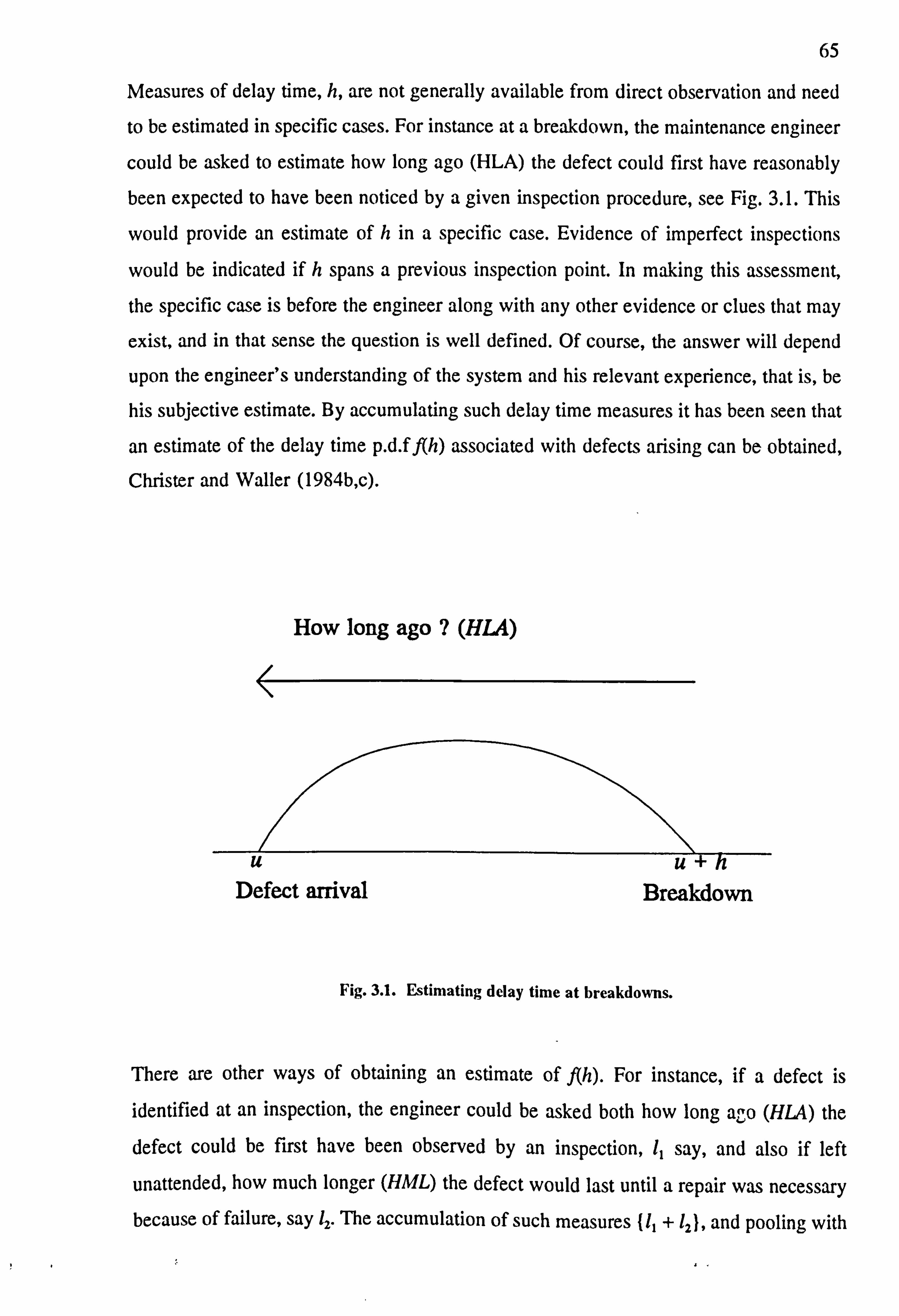
65

Measures of delay time, h, are not generally available from direct observation and need

to be estimated in specific cases. For instance at a breakdown, the maintenance engineer

could be asked to estimate how long ago (HLA) the defect could first have reasonably

been expected to have been noticed by a given inspection procedure, see Fig. 3.1. This

would provide an estimate of h in a specific case. Evidence of imperfect inspections

would be indicated if h spans a previous inspection point. In making this assessment,

the specific case is before the engineer along with any other evidence or clues that may

exist, and in that sense the question is well defined. Of course, the answer will depend

upon the engineer's understanding of the system and his relevant experience, that is, be

his subjective estimate. By accumulating such delay time measures it has been seen that

an estimate of the delay time p. d. f f(h) associated with defects arising can be obtained,

Christer and Waller (1984b, c).

How long ago ? (HLA)

u Defect arrival

u+n Breakdown

Fig. 3.1. Estimating delay time at breakdowns.

There are other ways of obtaining an estimate of 1(h). For instance, if a defect is

identified at an inspection, the engineer could be asked both how long aco (HLA) the

defect could be first have been observed by an inspection, 11 say, and also if left

unattended, how much longer (HML) the defect would last until a repair was necessary because of failure, say 12. The accumulation of such measures {11 + 12}, and pooling with

66

any breakdown based delay time measures, would lead to the estimation of a distribution

which is directly related to f(h).

A situation of censored data may arise. For example, the delay times of defects detected

at inspections may not be possible to estimate due to the necessary prediction of the

future time to breakdown, i. e the inspection time + HML. This will be discussed in the

next chapter. For the present, we will assume that a subjectively based estimate of the

delay time distribution may be available. Essentially, the availability of subjective data,

that is the willingness of those involved to collaborate with data collection experiments

and surveys, will influence the form of the delay time distribution selected. Considerable

care must be taken when collecting such estimates to ensure the questions being asked

are properly understood. It may also be necessary to invite the engineer to provide a

range estimate of HLA and HML. Eitherway, by perhaps by permitting and taking the

mean or otherwise, such as an optimistic and pessimistic measure, we assume a single

estimate of h (= HLA + HML) is available for each defect or breakdown considered.

How long ago ? (HLA) I How much longer ? (HML)

uiu Defect arrival Identified

Fig. 3.2. Estimating delay time for defects identified at inspections.

The system will be assumed to have been operated over a survey period of M

inspections of constant period T0, subject to the assumptions of Sections 2.4 and 2.5

namely:

67

(a) At time 0, the system is in a new or 'statistically new' state, that is defect

free.

(b) Defects arise, independently at a constant rate (HPP), with rate

parameter k, only over the operating (or up) time. A prior test on

estimates of it have been assumed, here, for the HPP assumption.

Essentially estimates of it would be obtained from the estimates of HLA.

(c) Delay times, h, are independent of defect arrival time, it, and are

distributed with the p. d. f f(h) and c. d. f F(h).

(d) A breakdown imposes a small amount of downtime compared to

inspection period, T, with expected value db, db « T.

(e) The expected value of breakdown cost is cb and the expected value of

defect repair cost is cd.

(f) Inspections are carried out with perfectness, (3, where ß is the

probability that a defect present at an inspection is detected and

consequently repaired.

The condition, db « T, is not necessary in the case of the UBI policy, but for the current

simplified model is necessary in the PBI case.

3.3 Need to Update Prior Model

It should be noted that the downtime models (2.18) or (2.36) are driven by specific

observable and measurable parameters such as; downtimes, di and db, by modelling

assumptions such as (3 =1 or ß#1, and, in this case, by the subjectively based

distribution F(h). Information relating to the observed level of overall downtime being

experienced under the existing operating conditions has not been specifically used. It is

a surprising fact that here we have been able to produce a downtime model for different

inspection periods which has been derived without considering the downtime levels

associated with the current practice, since conventionally the latter would be a starting

point for the former. That current experience appears not to have had an explicit

influence on the model is due, so far, to the mechanistic method of delay time analysis

adopted. Of course, we are utilising subjective assessments each of which is presumably

coloured by current experience.

6

Expected downtime per unit time, d(T)

a d(7a

b

T

Fig. 3.3. Comparison of estimated model, d(T), and possible observations.

The existing expected downtime levels should, and do, directly influence the model

through estimates of d, and db. However, these parameters, the delay time distribution

and the delay time model should also influence the model since it must be capable of

predicting the status quo situation, that is current practice. If, for example, an inspection

practice is to operate with a period To and the operating experience is of an average

plant downtime per unit time do*, then the curve of Fig. 3.3 should pass through the

point (To, d(To)). The chance of this subjectively derived point coinciding with the

observed point (To, do) is remote. What is expected to occur is typified by Fig. 3.3 in

which the observed point (To, do) could be in a position such as (a), or perhaps (b).

Effectively, d0*, is likely to be a periodic based estimate of a stochastic variable, and the

models of downtime presented here, are average value models of a stochastic variable.

If d, * is above (below) the curve then the delay time p. d. f chosen has most likely been

estimated with a higher (lower) mean value. The estimated defect rate, k or g(u),

modelling parameters, ß, for the probability of detecting a defect at inspection, and

estimates of the mean values of inspection and breakdown downtime, d1 and db, will also

influence the position of do' relative to the estimated model.

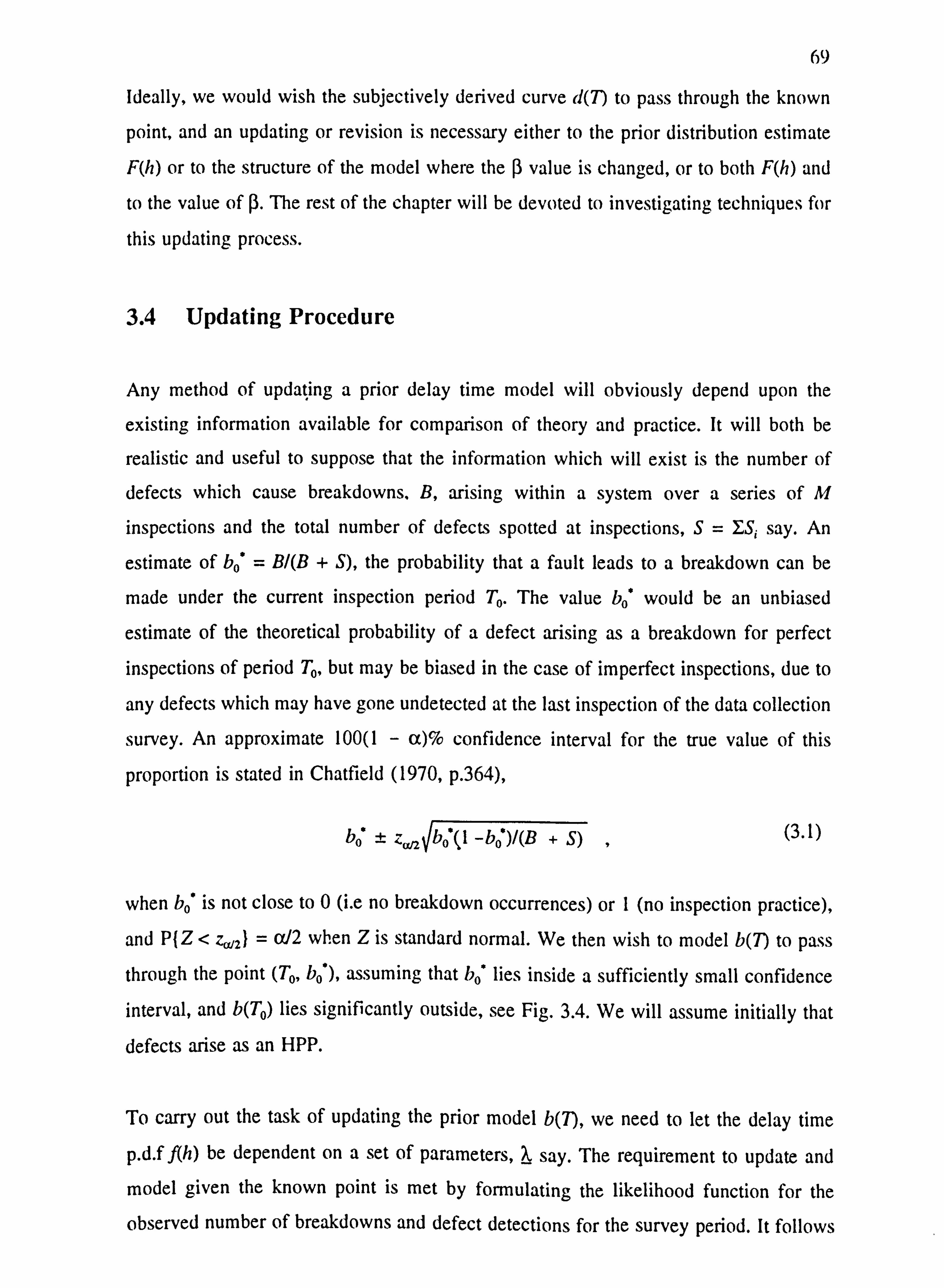
69

Ideally, we would wish the subjectively derived curve d(T) to pass through the known

point, and an updating or revision is necessary either to the prior distribution estimate

F(h) or to the structure of the model where the F value is changed, or to both F(h) and

to the value of P. The rest of the chapter will be devoted to investigating techniques for

this updating process.

3.4 Updating Procedure

Any method of updating a prior delay time model will obviously depend upon the

existing information available for comparison of theory and practice. It will both be

realistic and useful to suppose that the information which will exist is the number of

defects which cause breakdowns. B, arising within a system over a series of M

inspections and the total number of defects spotted at inspections, S= ES; say. An

estimate of b0 = BI(B + S), the probability that a fault leads to a breakdown can be

made under the current inspection period To. The value b0 would be an unbiased

estimate of the theoretical probability of a defect arising as a breakdown for perfect

inspections of period To, but may be biased in the case of imperfect inspections, due to

any defects which may have gone undetected at the last inspection of the data collection

survey. An approximate 100(1 - (x)% confidence interval for the true value of this

proportion is stated in Chatfield (1970, p. 364),

bo* ±z bý (l -bo*)/(B + S) , (3.1)

when b0 is not close to 0 (i. e no breakdown occurrences) or 1 (no inspection practice),

and P{Z < zß, 2} = a/2 when Z is standard normal. We then wish to model b(T) to pass

through the point (To, b(, ), assuming that bo* lies inside a sufficiently small confidence interval, and b(T0) lies significantly outside, see Fig. 3.4. We will assume initially that

defects arise as an HPP.

To carry out the task of updating the prior model b(7), we need to let the delay time

p. d. f f(h) be dependent on a set of parameters, ? say. The requirement to update and

model given the known point is met by formulating the likelihood function for the

observed number of breakdowns and defect detections for the survey period. It follows

70

from Section 2.5 that the number of recorded breakdowns, B. and defects detected, Si,

over the i'th inspection interval, are independently Poisson distributed with means

kTob(T0; 1) and kT0(1 - b(T0; 1) } respectively, when inspections are perfect. Hence, the

likelihood fui. ction over the survey period, given the observed B, breakdowns and Si

inspection identified defects in the i'th inspection cycle, L(ý) say, is given by,

e-kTo tTo: xi (kTob(To;? )) B ekr0(b(T0 1- i) (k To(1 - b(To; X )S, L() _

(3.2) 11 - B.! S,

Here, b(T; 1) is given by function (2.16) using the parameterized form of delay time

p. d. f j(h). By simplifying equation (3.2) and partially differentiating with respect to I

the corresponding log likelihood function, it follows that we need to solve,

b(To; ý) = B/(B + S) = bö ,

(3.3)

to obtain the maximum likelihood estimates (MLE) of X. It also follows that the MLE

for the rate of defect arrivals, k, when allowing k to be a parameter, is as expected,

B+S (3.4) MTo

Hence the proposed process to model the known point of current practice by equating

b(T0; 2) to bo* is equivalent to satisfying a requirement for a maximum likelihood fit of

objective data. Techniques to generate a set of parameters in order to revise or update

the prior model of b(T) are now considered.

3.5 Linear Delay Time Update

Here we consider the case when each estimate of delay time It for a defect is linearly

related to its actual delay time h' by,

h' = ah +co ,

where a and co are parameters to be estimated.

(3.5)

There are two restrictions on the parameter values of a and CO. First, it is assumed that

a>0, i. e.,

71

The probability a defect causes a breakdown, b(7)

16

b(1?

Fig. 3.4. Comparison of model, b(T), with known observation point.

a>0 , (3.6)

otherwise large estimates of h would transform to small actual values h' and vice-versa.

Secondly, h' must be non-negative so if ho is the smallest value of h for which the prior

distribution satisfies F(h) >0 for h> ho, then we require,

aho +w >_ 0. (3.7)

It follows that for any x, the probability P{h' <_ x} = P{h <_ (x - (0)/a}. Consequently

the parametric form for the c. d. f of h' is given by,

P{h'<_x} = Fx-w ,

(3.8) a

where F(h) is assumed zero for h <_ 0, which implies c. d. f (3.8) is zero when 0<_h' _aho+w.

Let the initial model b(7) be constructed with an estimate ßo for the probability of

perfect inspection, ß, and let b(T; (X, ci) be the updated parametric form for b(T) when

replacing F(h) by the transformed expression (3.8). Clearly we seek a set of parameters

(a, w) such that the status quo condition is satisfied, that is,

0 TO Inspection Period, T

72

b(T,,; a, (o) = b0 . (3.9)

Essentially we are seeking maximum likelihood estimates of the scale, a, and location

parameter Co of an assumed delay time p. d. f family based on numerous observations. We

now consider the possible existence of and uniqueness of solutions to equation (3.9).

3.5.1 Special Case: Scale Parameter, a, Update

Consider, first, the case when co = 0. It will be shown that a unique solution for a

exists. Now, if (30 = 1, the case of perfect inspection, to satisfy condition (3.9) with b(T)

given by function (2.16) and using the parameterised c. d. f (3.8), we seek a value a

satisfying,

T 40--(XX, J 4-ixi dx = hý (3.10)

Using the substitution x= ah and re-arranging, we have,

Twa (TWoc - h) (3.11) fTa f(h)dh = bo* h=0

where the left hand side of (3.11) is the model of b(T), function (2.16), with T replaced

by Tda. For a solution to equation (3.11), therefore, we require an a such that,

(3.12)

(l a

[l

The model b(7) increases monotonically from zero to one as T increases from ho to

infinity. Thus, since 0< )o' < 1, there exists a unique inspection interval T,, such that,

b(T1) = bo` .

(3.13)

It then follows that the unique solution for a is given by,

73

a= TO

(3.14) T,

The solution a can also be found graphically by scaling or shearing the model b(T), that

is, by translating each point IT, b(T) } to (T, b(T(T1/To)) }.

In other words, in the case of perfect inspections, ß=1, a unique transform of the delay

time h' = ah can always be made to satisfy a status quo observation on b(T), where

a= To/T, and Tt is the solution of equation (3.13). In the case when ßo < 1, it can be

seen that equation (3.9) is also appropriate for this case by using the substitution x= ah

in function (2.30). It then follows, as before, that a unique solution for a exists.

It also follows that,

b0 >b(T0)=Tl>To =cc <1, (3.15)

bö < b(T0) = T1 < To =a>1.

The main point here is that there exists a unique transform of the initial prior

distribution which will modify the model of b(7) to satisfy a known status quo

observation for (30 <_ 1. An example of this formal updating is given below.

Example. The following example is based upon a case study for a canning line,

Christer and Waller (1984b). For this situation we let,

To = 24 hrs,

f(h) = 0.0447. exp(-0.0447h), (exponential),

ßo = 1, (perfect inspections),

db = 0.698 hrs,

di = 0.525 hrs,

bo` = 0.390,

k=0.101 hrs-`.

In the study it was found that, b(T0) = 0.387, which was not felt significantly different

from bo` to warrant updating. This is envisaged to be a rare occasion because the model

I

74

b(T0) is subjectively derived, whereas the number 0.387 reflects observation. For

demonstration purposes, we consider two extreme cases here, one of over estimating and

one of under estimating, namely, we suppose two levels of observed downtime,

(a) bo` = 0.2

and

(b) b0 = 0.6

and update the model of b(T) using the transform h' = ah. Case (a) represents an

observation significantly less than the prior model value b(T0) = 0.387, and case (b) is

correspondingly significantly greater. Hence, the equation for a, (3.10), takes on the

form,

24 ('(24 - x) 0.0447

exp(-0.0447x/a)dx = bý , (3.16)

x=0 24 a a

which on integrating the L. H. S. of equation (3.16), simplifies to,

exp(-1.0728/a)) _b.. (3.17)

1.0728 -o

This equation can be shown to have the following respective solution for case (a) and

case (b),

(a) a=2.304,

(b) a=0.481.

To demonstrate the effect of these updates, the initial model of b(T) is shown in Figs.

3.5 and 3.6, with the scale update model for cases (a) and (b) respectively. The updated

curves for b(7) clearly pass through the known point (24,0.2) and (24,0.6) as required,

that is the curves satisfy the status quo condition (3.9).

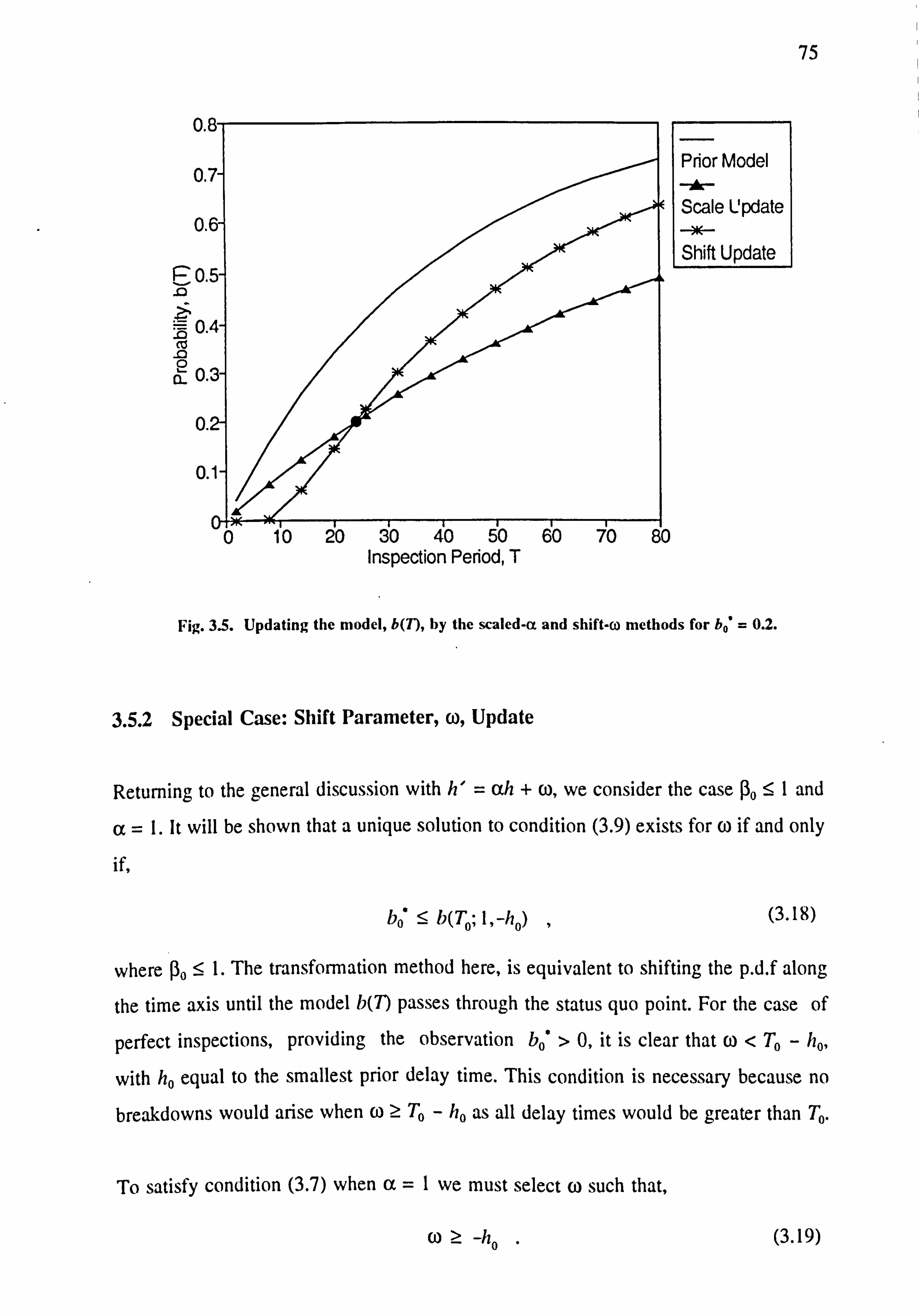
75

B v

M (10 .n 2 CL

Prior Model

Scale Update

Shift Update

Fig. 3.5. Updating the model, b(7), by the scaled-a and shift-w methods for bo' = 0.2.

3.5.2 Special Case: Shift Parameter, w, Update

Returning to the general discussion with h' = ah + co, we consider the case ßo <_ 1 and

a=1. It will be shown that a unique solution to condition (3.9) exists for 0 if and only

if,

boy ý b(T0; 1, -ho) , (3.18)

where (30 <_ 1. The transformation method here, is equivalent to shifting the p. d. f along

the time axis until the model b(T) passes through the status quo point. For the case of

perfect inspections, providing the observation b0* > 0, it is clear that CO < To - ho,

with ho equal to the smallest prior delay time. This condition is necessary because no

breakdowns would arise when w >_ To - ho as all delay times would be greater than To.

To satisfy condition (3.7) when a=1 we must select co such that,

w? -ho . (3.19)

Inspection Period, T

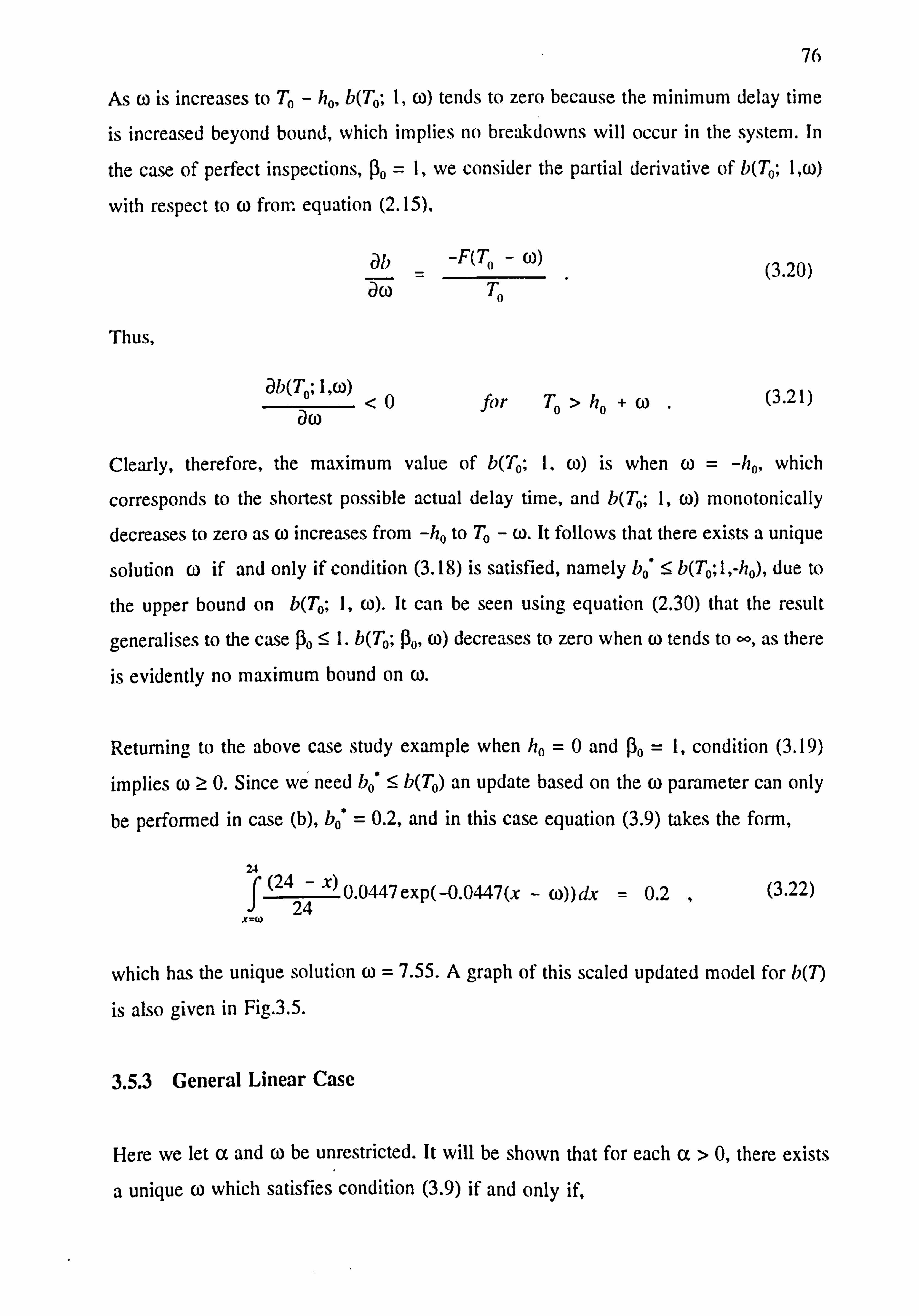
76 As w is increases to T. - ho, b(T0; 1, w) tends to zero because the minimum delay time

is increased beyond bound, which implies no breakdowns will occur in the system. In

the case of perfect inspections, ßo = 1, we consider the partial derivative of b(T0; 1, w)

with respect to co from equation (2.15).

ab -F(TO - co) (3.20) 7w- TO

Thus,

ab(To; l, w) <0 for To > ho + (3.21)

aw

Clearly, therefore, the maximum value of b(T0; 1, w) is when co = -ho, which

corresponds to the shortest possible actual delay time, and b(T0; 1, (0) monotonically

decreases to zero as to increases from -ho to To - co. It follows that there exists a unique

solution co if and only if condition (3.18) is satisfied, namely boo <_ b(To; 1, -ha), due to

the upper bound on b(T0; 1, co). It can be seen using equation (2.30) that the result

generalises to the case ßo <_ 1. b(T0; (30, co) decreases to zero when co tends to oo, as there

is evidently no maximum bound on co.

Returning to the above case study example when ho =0 and (30 = 1, condition (3.19)

implies co >_ 0. Since we need bo* <_ b(T0) an update based on the co parameter can only

be performed in case (b), bo* = 0.2, and in this case equation (3.9) takes the form,

24 (' (24 - x) 0.0447exp(-0.0447(x - cw))dx = 0.2 ,

(3.22) X-

24 ý

which has the unique solution to = 7.55. A graph of this scaled updated model for b(T)

is also given in Fig. 3.5.

3.5.3 General Linear Case

Here we let a and w be unrestricted. It will be shown that for each a>0, there exists

a unique co which satisfies condition (3.9) if and only if,

77

E

sM .0 0 a

Prior Model A Scale Update

Beta Update

Fig. 3.6. Updating the model, b(T), by the scaled-a and revised-n methods, b0* = 0.6.

bo* 5 b(To; (x, -aho) , (3.23)

where w >_ -aho and (io < 1.

To satisfy condition (3.7) we require (o > -aho, which gives the maximum value of

b(T0; a, co) with respect to w. Due to a>0, the partial derivative (3.20) of b(T0; a, co)

with respect to 0 will still be negative. In the case (30 = 1, the maximum bound of u0

would be To - aho because all transformed delay times, h', would be greater than To,

implying no breakdowns would arise (assuming bo' # 0). For the case Do < 1, b(T0; a, co)

tends to zero as w tends to 0. Hence, condition (3.23) above is both necessary and

sufficient.

It is interesting to show, here, that for the case of perfect inspections, a relationship

exists between the parameters (a, w) selected and the updated delay time mean. If p is

the mean of the prior distribution F(h, ) then the mean of the transformed distribution,

µ' say, is given by,


79

µ' =aN+ Co . (3.24)

In the case ßo = 1, to satisfy the known point we can also solve, using function (2.15)

for b(T), the equation.

To(I - b0) = j[i

- 1.

' aw

Jjdx . (3.25)

Xo

The R. H. S is the integral of the survivor function, which tends monotonically to µ', as

To tends to oo. Therefore, the L. H. S would be less than the delay time mean value.

Hence, we obtain the relationship,

P/ = aµ +w > T0(1 -bo) . (3.26)

which provides a lower bound for the delay time mean, assuming that bo' is known to

a sufficient degree of accuracy and modelling assumptions are valid.

3.6 Model Parameter Variation

In this case we now allow I to vary in the prior maintenance model, which is denoted

by the probability function (2.30), b(T; ß), and we seek a value (3 such that,

b(T0; ß) = b, )* . (3.27) That is, we now seek to satisfy the status quo condition on the assumption that it was

the original modelling that was at fault in assuming that inspections were or were not

perfect, i. e selecting the wrong value for (30.

The minimum value of b(T0; ß) corresponds to ß=1, the perfect inspection model.

When (3 =0 we have b(T; (3) =1 for all T, and as shown with result (2.33) in Section

2.5.5,

ab(To; ß) (3.28)

for any value of P.

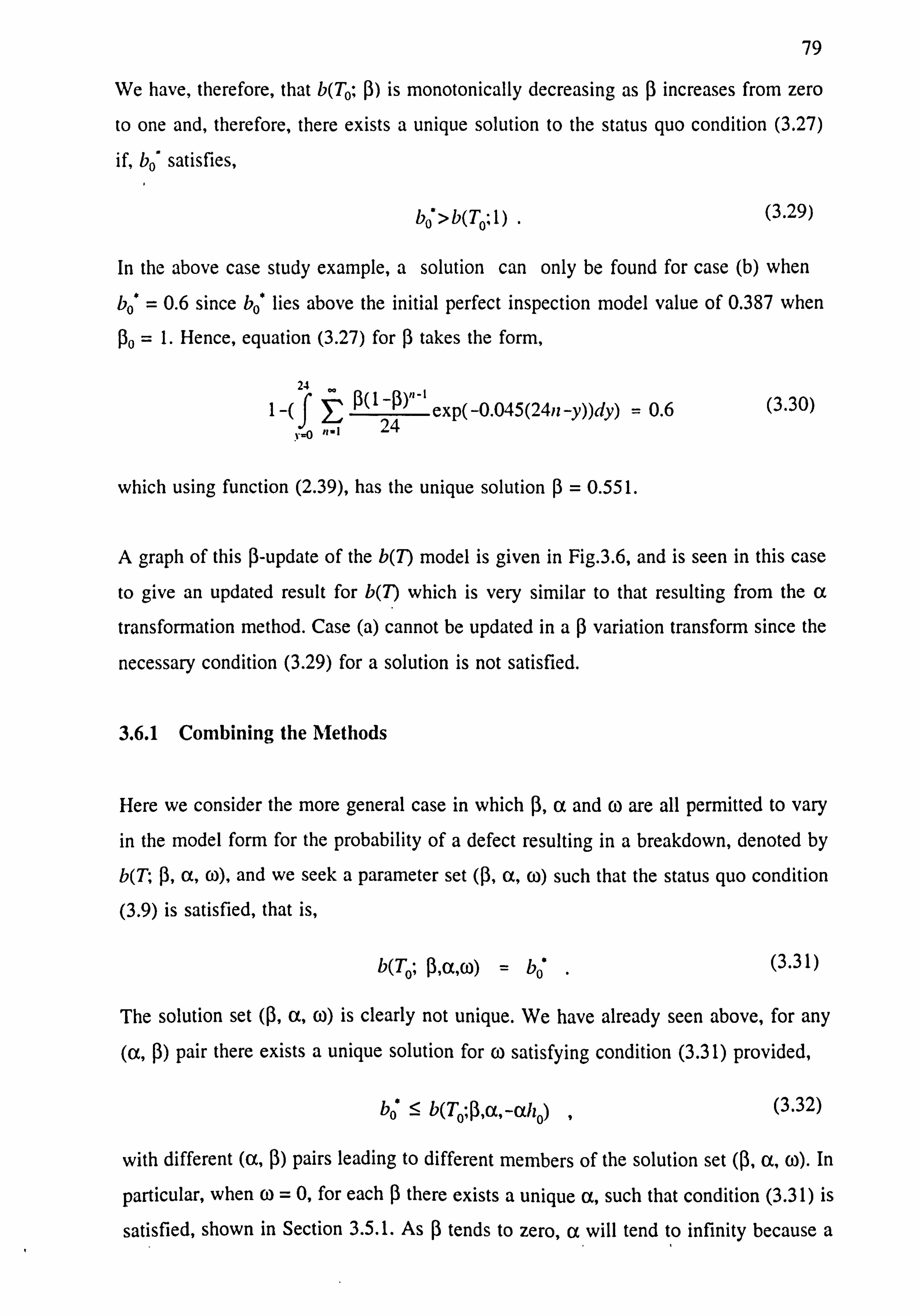
79

We have, therefore, that b(T0; ß) is monotonically decreasing as (3 increases from zero

to one and, therefore, there exists a unique solution to the status quo condition (3.27)

if, bo' satisfies,

b0 > b(To; 1) . (3.29)

In the above case study example, a solution can only be found for case (b) when

bot = 0.6 since bo* lies above the initial perfect inspection model value of 0.387 when 0a = 1. Hence, equation (3.27) for P takes the form,

1 _(ia E ß(1-ß)"-`

exp(-0.045(24n -Y))dy) = 0.6 (3.30) J ,,,, 24

which using function (2.39), has the unique solution (3 = 0.551.

A graph of this ß-update of the b(7) model is given in Fig. 3.6, and is seen in this case

to give an updated result for b(7) which is very similar to that resulting from the a

transformation method. Case (a) cannot be updated in aß variation transform since the

necessary condition (3.29) for a solution is not satisfied.

3.6.1 Combining the Methods

Here we consider the more general case in which (3, a and (1) are all permitted to vary

in the model form for the probability of a defect resulting in a breakdown, denoted by

b(T; ß, a, (), and we seek a parameter set (ß, a, w) such that the status quo condition

(3.9) is satisfied, that is,

b(T0; ß, a, w) = bö (3.31)

The solution set (ß, a, (o) is clearly not unique. We have already seen above, for any

(a, (3) pair there exists a unique solution for w satisfying condition (3.31) provided,

bo _< b(T0; ß, a, -(xho) , (3.32)

with different ((x, ß) pairs leading to different members of the solution set ((3, a, c)). In

particular, when w=0, for each 0 there exists a unique a, such that condition (3.31) is

satisfied, shown in Section 3.5.1. As ß tends to zero, a will tend to infinity because a

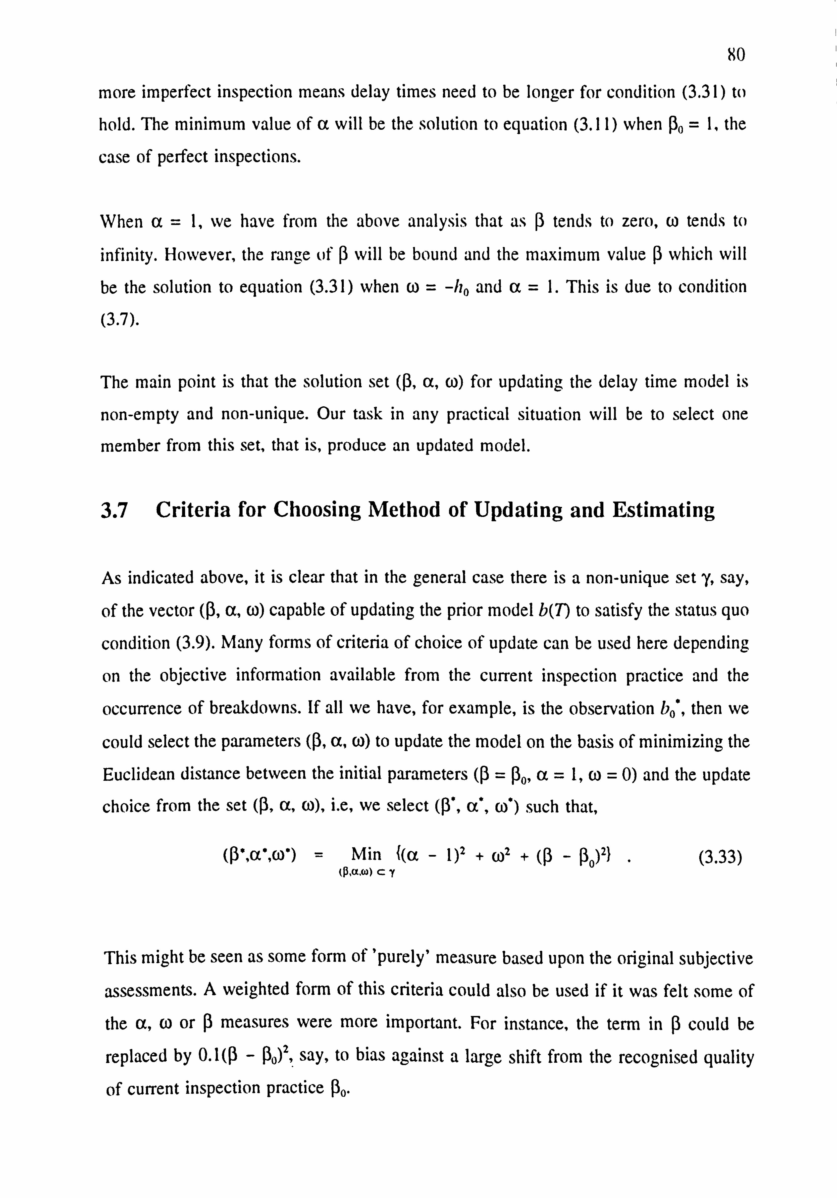
so more imperfect inspection means delay times need to be longer for condition (3.31) to

hold. The minimum value of a will be the solution to equation (3.11) when (30 = 1, the

case of perfect inspections.

When a=1, we have from the above analysis that as ß tends to zero, w tends to

infinity. However, the range of ß will be bound and the maximum value ß which will

be the solution to equation (3.31) when w= -ho and a=1. This is due to condition

(3.7).

The main point is that the solution set (ß, (X, co) for updating the delay time model is

non-empty and non-unique. Our task in any practical situation will be to select one

member from this set, that is, produce an updated model.

3.7 Criteria for Choosing Method of Updating and Estimating

As indicated above, it is clear that in the general case there is a non-unique set 'y, say,

of the vector (ß, a, w) capable of updating the prior model b(T) to satisfy the status quo

condition (3.9). Many forms of criteria of choice of update can be used here depending

on the objective information available from the current inspection practice and the

occurrence of breakdowns. If all we have, for example, is the observation b0*, then we

could select the parameters (ß, a, (o) to update the model on the basis of minimizing the

Euclidean distance between the initial parameters (ß = (30, (x = 1, w= 0) and the update

choice from the set (ß, a, (o), i. e, we select (ß', a`, co) such that,

(ß', a', ( 5) = Min {(a - 1)2 +0+ (ß - ßo)2} (3.33) (p, a, w) cy

This might be seen as some form of 'purely' measure based upon the original subjective

assessments. A weighted form of this criteria could also be used if it was felt some of

the a, w or I measures were more important. For instance, the term in ß could be

replaced by 0.1(13 - ßo)2, say, to bias against a large shift from the recognised quality

of current inspection practice ßo.

81 3.7.1 Method of Moment Parameter Selection

Another possibility for choosing a solution ((3', a*, w) from the satisfying set

arises from the observations of times of breakdowns, was mentioned in the papers

Christer and Redmond (1992). Accepting current practice, we can calculate the time

since the last inspection for each breakdown, y say. The moments of the breakdown

time, e. g mean and variance, can be estimated and set equal to parametric models of

such statistics. Then, the parameters (ß, a, w) can be selected to satisfy the set of

equations produced. In order to achieve this, we need to first derive the p. d. f of times

of breakdown.

Breakdowns arise as a NHPP, shown in Section 2.4. Therefore, the conditional p. d. f of

the breakdown time of a given random breakdown, pb(y; 7) say, is given by,

Pb(Y; 7) _ __ for 05y<T, (3.34)

where B(T) is the expected number of breakdowns in interval (0, T) and r(y) is the

ROCOF for the system after time 0. In the case of perfect inspections, r(y) = B' (y). The

corresponding result to the breakdown time distribution (3.34) can be found in Parzen

(1962, p. 145) and Ascher and Feingold (1984, p. 32).

For perfect inspections (ßo = 1) and HPP defect arrivals, r(y) = kF(y), and using function

(2.15) the p. d. f Pb (y; 7), equation (3.34), then takes on the form,

Pb(Y: = F(y)

= F(y)

Tb(T) T (3.35) 5F(y)dy

r=o

The function pb(y; 7) can be seen to be non-decreasing function over the interval

yc (0,7). Hence, it is anticipated that bounds can be attached to the mean value of y. The p. d. f with the least mean value would be the uniform distribution when all delay

times of defects are zero. Hence, defining the mean breakdown time by M(7), we have,

T

M(7) Tb(7)

fyF)d)' T (3.36) y=0

82

Also since F(y) <_ 1, we have M(T) <_ T/(2b(T)). Due to the p. d. f (3.35) being

numerically equal to the delay time c. d. f divided by its integral over the interval (O, T'),

a method of obtaining a prior delay time c. d. f could also be obtained from observation

of failure times. E. g if 1)^(v) is the sample p. d. f of breakdown times, an estimate of the

c. d. f of delay time is F y) = T0b0`jA"yv), for 0 <_ y <_ T, assuming that 1) (Y) is

monotonically increasing. Consequently the model 1)(T) and subsequently B(T) can be

estimated for 0: 5 T STo.

In Section 3.5, it was shown that there exists a non-unique set (a, () to update the

model b(7). If an estimate of the mean time of breakdown is available, ino` say, then it

follows, using the above p. d. f (3.35), that we need to solve,

ra 1 fvF(cxv

+ w) dy = 11107 . (3.37)

b(To; a, w) Ta V, -0

in addition to solving the condition (3.31). We are in effect seeking values for a and w

such that the mean time of breakdown and the proportion of defects arising as

breakdowns satisfy the observed current inspection practice, To. Clearly, we require

ino' > Tß/2 for the existence of a solution. This proposed method is demonstrated using

simulated data in Chapter 5. Clearly, the method could also be extended to imperfect

inspections by using the sample estimate of the variance of breakdown times to give

three equations to solve for ß, a and co.

3.7.2 Maximum Likelihood Parameter Selection

The maximum likelihood method of estimating parameters, in general, gives more

efficient estimates, i. e they become closer to the true theoretical value of the parameters

rapidly as the sample size increases, see Edwards (1972). If Nb breakdowns have

occurred over the interval (0,7) and {y, }, 1 _<

j <_ Nb, are the failure times measured

from 0, then due to NHPP breakdown arrivals, the likelihood, L say, is given by,

83

A

Np

Li = exp(-B(T))[J r(y, ) , (3.38)

i-I

shown in Cox and Hinkley (1974) for the NHPP. The functions r(y) and B(7) can then

be parameterized in terms of (ß, a, (o). For the case of imperfect inspections the

ROCOF would need to be formulated for each inspection interval over the survey

period. This can be achieved by deriving the expected number of breakdowns, Bn(y; 7)

say, occurring in the interval (0, y) after the n'th inspection. The ROCOF for the n'th

interval from when the system was new can then be obtained by differentiating this

function w. r. t y. If times of failures have not been recorded then an alternative likelihood

can be formed from the observed number of breakdowns within each inspection interval.

This likelihood would be constructed using function (2.32), that is the expected number

of breakdowns, B�(7), occurring in the n'th inspection interval.

Over the series of inspections, the likelihood of each interval would be combined, and

this can then, also, be multiplied with the likelihood of the number of defects recorded

at each inspection, based on the Poisson distribution. The combined likelihood for

perfect inspections, using the notation in Section 3.2, is then given by,

E S` -MS(To) IN 'S(TO) e

-MB(T B

L= Al e °ý r(yj) (3.39) i

ll Si j=1 !

i-1

where B(T) is the expected number of breakdowns in an inspection interval (0,7) and

S(T) is the expected number defects to be detected at each inspection. The function

(3.39) can then be simplified to (omitting constant factors),

L3= K(7)se -MK(7)(1 B

- ý(T))S rl r(y j) j=1

(3.40)

where K(7) is given by function (2.7). In the case of assumed HPP defect arrivals then

r(y) = kF(y), the likelihood factorizes to give,

84

B

b(7))' Il F(y) (3.41)

, _I The parameters can then be selected to maximize over the resulting likelihood (or log-

likelihood) function. This process will be demonstrated using simulated data in Chapter

5. When inserting the selected parameters into the function b(7), the status quo condition

will not necessarily be modelled exactly. Clearly, if modelling assumptions are correctly

postulated the estimated value b(T0) should lie within confidence limits of bo Modelling

assumptions will need to be revised in the case when this is not so.

The method to use objective data has been used for estimating the delay time

distribution of a single-component system, see Christer and Wang (1992), Baker and

Wang (1992).

3.8 Statistical Tests of Fit

A list is given here on the ways of testing the selected model, assuming that

parameters ((3, a, w) have been estimated using any of the methods outlined in Sections

3.5,3.6 and 3.7:

(a) Satisfying the known point, b0*.

(b) Chi-square test or Kilmogorov-Smirnov test, based upon the number of breakdowns in each interval being Poisson distributed.

(c) As in (b), but for the detected defects at inspections.

(d) As in (b), but where the times of failures have the p. d. f pb(y; 7).

(e) Satisfying the sample mean time of failure, nzo'. (f) Satisfying the sample variance of time of failure, vo* say.

If in a practical situation, all tests (a)-(f) are positive, then the belief is reinforced that

modelling assumptions and updating procedures are valid for the system in question.

If many tests are negative then we could infer that defects may not be HPP, in which

case a time dependent form of the rate of occurrence of defects should be sought. Also,

85 linear updating may not be appropriate. E. g, the delay times defects which caused

breakdown under an assumed perfect inspection policy may be more accurately

estimated than delay times captured at inspections. The p. d. f type for delay time may

also be wrongly selected.

3.9 Other updating methods

The section outlines other updating methods for further research. For example, a non-

linear delay time transformation could be applied, such as,

hI = ah1 + Co . (3.42)

In this case, if h was initially estimated as being exponential, then the true delay time

h' would be distributed as a three parameter Weibull.

Alternatively to this method, one could select different standard parametric distributions

for the delay time distribution, e. g Weibull and Gamma, use maximum likelihood

estimation for the parameters given the observations, and then carry out the goodness-of-

fit tests outlined in Section 3.8.

In general, it could be assumed that there exists a conditional p. d. f of the actual delay

time, h', given a subjective estimate h, say ff(h'; h). It then follows that if f(h) is the

prior p. d. f of delay time subjective estimates, then the p. d. f of delay time, say f (h' ), is

given by,

f'(h ') = ff(h'; h)f(h)dh (3.43)

h=0

For the case of the delay time non-linear transform, the c. d. f form of L(h'; h) would be

the Heaviside function H(h' - (ahl+ w)).

3.10 Decision Consequence

Having discussed the updating and testing of fit, we now consider the decision

consequence of the various updating procedures. That is, how would the optimal

86

decision for d(7), say, change with the update and how different is the actual associated

d(T) value. We shall consider this in the context of the above case example.

b V

c

aD 0- G)

c 0 a aý U U d X

W


Prior Model -A- Scale Update -)K Shift Update

Fig. 3.7. The decision consequence, d(T), for update methods a and w.

First, we shall look at case (a) when bo' = 0.2. In Fig. 3.7 the graphs for d(T), equation

(2.18), using the delay time distribution update methods based on a-scale and w-shift

are shown. The point at which the update methods intersect, would be the estimated

downtime per unit time do' for the current practice To, where the values of bo', k, db and

(1, are estimated over the same time survey time period, that is M(T0' + d1), for which

do' is estimated i. e,

d' = kTodbbo + d`

0 To +dt (3.44)

The initial model has its minimum around T= 24 hours, for the actual current practice.

Whilst the minimum for the a-scale update model is greater, around T= 36 hours, it is

evident that the co update model is slightly less. Considering the two methods, it can be

seen the optimal region is probably between 20 and 40 hours. Although the downtime

87

I-

N E :r

n a) E c 0

U N 4 X

Prior Model

Scale Update -*- Beta Update

)

Fig. 3.8. The decision consequence, d(7), with the update methods a and P.

consequences over this range from 20 to 40 indicate that considerable care needs to be

taken in selecting an updating method. Secondly, we shall look at case (b) when b0' -

0.6. In Fig. 3.8 the graphs for d(T) using the update methods based on a and 0 are

shown. It can be seen that minimal change of the optimum value of d(T) has resulted

from these updates. Also, the change in d(T) is very slight as T ranges from 10 hours

to 120 hours and the value of d(7) is close to the limiting value of b(T) for large T,

which is kdb = 0.07 in this case. The value of kdb, as shown in Chapter 2, represents the

approximate expected downtime per unit time experienced under a breakdown

maintenance scheme, and so for case (b) inspections may be considered, in the example,

not to have much impact on reducing downtime as T increases beyond 24 hours.


88 3.11 Conclusion

Several formal techniques of updating delay time models have been presented. These

have been based on the existence of subjective data to decide a prior or type of delay

time distribution. The prior is then parameterized under a linear transform and the

uniqueness and existence of a solution to modelling the "status quo" discussed. It has

been found that a unique solution exists under a simple scale transform and a set of

solutions under the more general linear case. The effects of changing the model, that is

for 1=I to 13 : P--L I and vice-versa, or simply varying ß, as another updating option has

also been investigated which highlights the variety of updating options.

The effects of the change in the downtime model and consequently the optimum

inspection period has been demonstrated for various updating techniques. Further

research could lie in predicting the behaviour of the optimum for updating options,

modelling parameters and delay time p. d. f types.

Another method of parameter estimation has been proposed based on observed times of

breakdown and the defects detected at inspections. For this method, the prior distribution

type can be assumed and the parameters are then determined using the method of

moment or maximum likelihood technique. It has been seen that the observed failure

times can be also be used in a test for fitting a model and in deciding upon a delay time

prior when no delay time data is available.

Delay times may not only be biased subjectively, but also through estimates being drawn

from a censored data set. Delay times, for example, may only be estimated from the

failures which occur over a data collection survey. Hence, an observational bias enters

the problem. The existence of this type of bias will be discussed in the next chapter

along with methods for its resolution.

89

Chapter 4

Bias in Delay Time and Initiation Time

Parameter Estimates for Censored Data

4.1 Introduction

In this chapter, the case of having a censored data sample with which to estimate a

delay time distribution is discussed. As previously outlined, one situation which could

arise is that delay times and initiation times of defects may only be readily estimated

from either breakdown events or when defects are detected at inspections. Another

situation could be a non-balanced mixture of these two extremes in that we may not be

able to obtain an estimate of delay time and initiation time for each defect which has

arisen over a survey period.

In the case of censored data, a bias in the estimated distribution of delay times or

initiation time would exist. This will be established by deriving the respective

conditional p. d. f of delay time and initiation time associated with defects which arise as

breakdowns, and those which are detected at inspection. The p. d. fs will be derived for

both perfect and imperfect inspection policies. A maximum likelihood estimation

technique and appropriate tests of model fit are then recommended to cope with the

observational bias introduced.

Much of the work of this chapter is based on the paper, Christer and Redmond (1990).

4.2 Bias in Delay Time Estimates

Practical applications of delay time analysis have so far exhibited the usual

characteristics of any initial exploration or application of an applied scientific idea. The

90

approach has been pragmatic in style in an attempt to obtain initial order-of-magnitude

effects and feedback prior to refinement. Delay time estimates, h, have, for example,

been derived by estimating both the delay time associated with a breakdown, hb = HLA

(How long ago the defect first arisen) say, and that with the inspection repair of a

defect, h, = HLA + HML (How much longer if left to deteriorate), see Figs. 4.1 and 4.2.

These two data sources have then been pooled and the prior p. d. f, j(h) estimated and

appropriate analysis undertaken, see Christer and Waller (1984b).

Delay Time, hb How Long Ago (HL4)

Ub

Defect arrival

ub+ hb

Breakdown

Fig. 4.1. Delay time estimated at breakdown.

In following this initial process, it is recognized that apart for a possible bias in

individual estimates of delay time associated with the individual providing the estimate,

an additional statistical bias may enter into the modelling.

To demonstrate this we initially assume perfect inspections and estimates of h= hb are

only obtained at breakdowns. Here, a set of estimates of hb will generally produce

parameter estimates which underestimate the p. d. f of h, due to the delay times, hb, all being constrained to be less than T. Further, a set of estimates of hd, will produce an

overestimate of the p. d. f of h, due to sampling at T which gives rise to a higher chance

of estimating a longer delay time. This effect ties in with length-biased sampling discu ; sed by Cox (1957,1.65) and with the w, i, -ing time paradox, s--c Feller (1970b).

91

Delay Time, hd = HLA + HML

How long ago ? (HLA) I How much longer ? (HML)

äI Udtnd

Defect arrival Identified

Fig. 4.2. Delay time estimated at inspections.

We imply here, that if pb is the expected value of hb and µd is the expected value of hd,

then we infer that Nb <_ µ and Pd >_ p, where p is the expected value of h. Strict inequality

will apply in most cases. These hypotheses will be proved in the following sections. We

shall deal first with the distribution of delay times based upon estimates captured at

breakdowns, hb, and then with delay times based upon inspection based estimates, hd.

4.2.1 Delay Times associated with Breakdowns

Initially, assume a perfect periodic inspection policy T with defects having delay times

distributed with p. d. f f(h) and the conditional initiation times, it, having p. d. f q(tt; T),

It e (0, T). It is also assumed that breakdowns are repaired with negligible time. We then

wish to calculate the p. d. f of the delay times captured at breakdowns, hb, say fb(ý; 7'. All

the delay times would evidently be less than T. Hence the p. d. f will have its domain

over the interval (0, T). We are, in effect, dealing with a conditional p. d. f, the condition

being that a defect causes a breakdown.

Consider the probability of the event, { hb e (ý, ý+ dý) }, for any ý, that is, fb(ý; T)dE for

small dý. If we now let b be the event that a defect leads to a breakdown when

92

inspection is on period T, and let H be the event that the delay time, h, of a defect

satisfies, he (ý, ý+ dý), it follows that,

P{hb c (ý, ý+ dý)} = P{Hlb} .

Using Bayes' theorem, we have for P(b) >0 the relation.

P{H I b) - P{H, b} P{H} P(b I H)

PT)-- P{li

(4.1)

(4.2)

In the case P{ b}=0 there is no data set { hb } to consider, and for the current case,

therefore, we assume P{ b}>0. We have by definition that the probability of H is

f(ý)dý. Therefore, if we let dý tend to zero in equation (4.1), using result (4.2), we can

obtain the formula,

fb( '' = f() P(b Ih =) (4.3)

Tv-

The probability of b is b(T), which is given by function (2.29),

T

b(7) =f Q(T - h; 7)f(h) Ah , (4.4)

h =0

where Q(u; T) is the c. d. f of u. It remains to calculate, P{blh = ý}, the probability that

a defect leads to a breakdown given delay time h=ý. If ý>T the defect would be

detected by an inspection, assuming inspections are perfect. If ý<T the defect would

cause a breakdown if the initiation time u<T-ý, which is an event with probability

Q(T - ý; 7'). Hence we obtain the p. d. f over the domain (0,7),

fb(ý _) Q(T ý; 7) fror 0<<T (4.5)

A c. d. f form of this p. d. f, Fb(ý; 7) say, was derived in Christer and Redmond (1990),

namely,

FA; 7_G F(ý)Q(T - 4; +

1

T f

q(u; T)F(T - u)du u=T-E,

E<T 9

'? T (4.6)

93

and is equivalent to the integral of function (4.5).

We can investigate the mean p. of f, (ý: 7) by noticing that the function Q(T - ý; T)

monontonically decreases from I to O as ý ranges from 0 to T. Therefore, there exists

a unique value '=0 such that Q(T - 0: 7) = b(T). Evidently, the p. d. f fb would lie

above f over the interval (0.0) and below f over the interval (0. T), see Fig. 4.3 for an

example. %%-hereby 0 is the delay time value at the intersection of the three p. d. fs. It

follows that the c. d. f of h, will lie above the c. d. f of It over the interval (0,0). Hence,

the associated reliability function (r. f) of hp will lie below the r. f of fi over this interval.

It can be readily seen that over the interval (0,7), the r. f of hb will also lie below the

r. f of h. It is a well known result that the mean of a non-negative random variable is the

integral of its r. f. Hence. we obtain the expected result.

tu (4.7)

that is the delay time parameter estimates associated with failures are biased. Clearly,

as T -* -, f -' f, that is estimates of he becomes asymptotically unbiased with T. An

example of bias is pnivided by the special case when delay times are exponential and

defertc arise uniformly as a HPP. Let a= I/p be the exponential parameter, then we

obtain from equation (4.4).

a a(T - ý)e~, fi)r 0<<T. (4.8) ` aT +e" -I

As anticipated. it can be seen that f, -a f as T -4 ca by replacing e"1T by its Maclaurin

series. A numerical example is given in Fig. 4.3 for T= 10 and a=0.2. The mean Pb in

this case is equal to 2.38, whereas p=5. It is evident here that the biased p. d. f of h can

be radically different from the true distribution.

3.2.2 Delay Times associated %iith Inspected Defects

In this case. we seek the p. d. f, say f (ý; 7). of delay times, hi, which span the inspection

point T. again assuming the inspection at T is perfect. That is we require the conditional

p. d. f of delay time given a defect is detected and repaired at the inspection T. Let d be

the event that a defect is detected at an inspection, then by following the process of

analysis leading to equation (4.3), it can be shown that for P(d) > 0,

94

0

0

0

a

Unconditional

Breakdowns -*- Inspection repairs

Fig. 4.3. An example of unconditional and conditional p. d. fs of delay time.

fd(ý = fý )PW I h=ý) if P(d) >0

(4.9) P(d)

We have for a defect that P{d} =I- b(7), and therefore need to consider the

probability Pfd Ih= ý}. For the case, ý>T, we have that Pfd Ih= ý} = 1, i. e the

defect will be detected given its delay time is greater than T and the inspection is

perfect. When E<T, then the defect will be detected if its initiation time satisfies

u>T-4, which is an event with probability 1- Q(T - ý; T). Hence, the required p. d. f

of detected delay times is given by,

f(ß)(1 - Q(T - i; 7)) 1- b(T)

fA; 7)

1- b(T)

for 0<4<T

for ; >_T .

(4.10)

As T -+ 0, it can be seen fd -4 f, that is hd becomes asymptotically unbiased as

inspections become more frequent. This behaviour is to be expected. A c. d. f form of fd,

02468 10 12 14 16 Delay Time

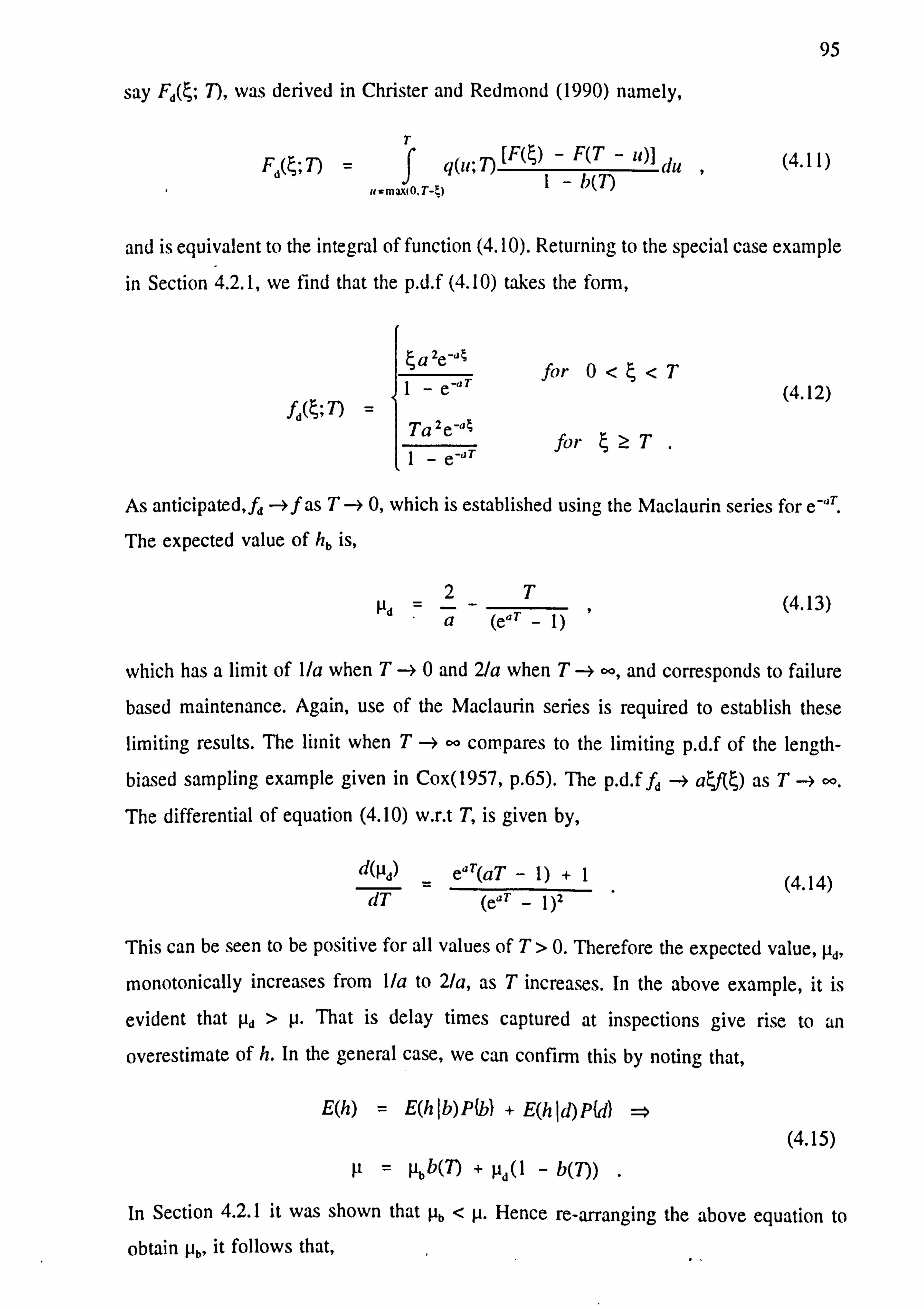
95

say Fd(ý; T), was derived in Christer and Redmond (1990) namely,

T

Fd(; T) = q(u; 7) [F(ý) - F(T - u)] A (4.11) u=maX(O. T-ý) I- b(7)

and is equivalent to the integral of function (4.10). Returning to the special case example

in Section 4.2.1, we find that the p. d. f (4.10) takes the form,

a 2e-4

1- e' r fill;

lJ

Ta 2e-°4

1 -e -aT

for 0<? <T (4.12)

for ý>_T

As anticipated, fd -4f as T --ý 0, which is established using the Maclaurin series for e-° '.

The expected value of hb is,

2T (4.13) µd (eaT - 1) ,

which has a limit of 1/a when T -4 0 and 2/a when T -* oo, and corresponds to failure

based maintenance. Again, use of the Maclaurin series is required to establish these

limiting results. The limit when T --3 oo compares to the limiting p. d. f of the length-

biased sampling example given in Cox(1957, p. 65). The p. d. f fd -4 af(t) as T

The differential of equation (4.10) w. r. t T, is given by,

d(µ) e°T(aT - 1) +1 (4.14) dT (eaT _ 1)2

This can be seen to be positive for all values of T>0. Therefore the expected value, µd,

monotonically increases from 1/a to 2/a, as T increases. In the above example, it is

evident that µd > p. That is delay times captured at inspections give rise to an

overestimate of h. In the general case, we can confirm this by noting that,

E(h) = E(hlb)P{b} + E(hld)P{d} (4.15)

V= pbb(7) + µd(1 - b(7))

In Section 4.2.1 it was shown that Pb < p. Hence re-arranging the above equation to

obtain Pb' it follows that,

96

Pb b(T))

Pd µ, (4.16) b(T)

Hence, in the general case the delay times of defects captured only at inspections are

biased with an expected value greater than the delay time mean. A numerical example

when T= 10 and a=0.2 is also given in Fig. 4.3 with p. = 8.34. It can be seen that all

three p. d. fs intersect at the same point. The delay time at this point (0 = 4.34), is such

that a defect with this delay time value will have probability Q(T - 0; 7) = b(T) of

causing a breakdown, and it can be seen that the delay time p. d. f in equations (4.5) and

(4.10) at ý=0 will equal f(0).

4.3 The Bias in the Initiation Times

We shall proceed to derive the p. d. fs of the initiation time associated with failures and

defects repaired at inspections. It will then be shown that the initiation time parameter

estimates are also biased under censored data. This is reasonable to expect, because the

initiation times of, for example, breakdowns, would be more likely to occur in the first

half of the inspection interval under a perfect inspection policy. In the case of inspection

identified and repaired defects, the initiation time would more likely to be in the latter

half of the inspection interval.

Let qA; 7) be the p. d. f of initiation time, ub say, for defects which result in failures,

where ýC (0, T). It follows from analysis in Section 4.2.1 that the p. d. f would be given

by,

9b(ß; fl = 9(c; ) P{h ju =t? (4.17) b(7)

Essentially, h has been replaced by u and f by q in function (4.3) due to independence

between u and h. Given the initiation time of a defect, u=ý, the defect will cause a

breakdown if its delay time h<T-C, which is an event with probability F(T - ý).

Therefore, the p. d. f of irb is given by,

97

9b(ß; T) _ 9(C; 7) F(T - C) b(T)

for 0<ý<T. (4.18)

We shall now investigate the mean of ub, say tab. In Section 2.5.5, it was shown that for

perfect inspections, b(7) S F(T). Hence the p. d. f qb lies above or at q at ý=0. At

ý=T, the p. d. f then must lie below or at q, since F(T - ý) is a monotonically

decreasing function. In the strictly decreasing case, there will exist only one point 0 such

that F(T - 0) = b(T). Hence, it follows from analysis on the conditional p. d. f fb, in

Section 4.2.1, that if the mean of the initiation time is tj then,

l1b <1 (4.19)

That is the initiation times of defects which cause breakdowns are biased with an

expected value less than the population initiation time.

The initiation times of defects which are detected and repaired, say ud, will also be

biased. In order to calculate the p. d. f of ud, it is evident from previous arguments that

we require the probability that a defect will be detected given its initiation time, it = ý,

that is P{dI it =ý}, for ýc (0,7). In this case, it is clear this is the probability that a

delay time satisfies h>T-ý, which is given by 1- F(T - ý). Let qd(C; 7) be the p. d. f

of ud, then as before it follows that,

ýd(P) = R(ý; T) [1- F(T - ý)J

1- b(7) (4.20)

To show the expected bias exists, we can follow a similar argument to that used in the

case of breakdown initiation times. Alternatively, if we let tad be the expected value of

ud, then,

that is,

E(u) = E(ulb)P{b} + E(uld)P{d} ,

T, = 11bb(7) + ld(1 - b(7'))

(4.21)

(4.22)

Hence, due to the fact that 1lb < T, we obtain the result,

98

11d > 11 1 (4.23)

that is the initiation times of defects which are repaired at inspections will be biased

with a greater expected value.

4.4 Imperfect Inspections (ß # 1)

Here we relax the condition of perfect inspections and seek the p. d. fs of delay time and

initiation time, for breakdowns and inspection repairs. It will be assumed that the

probability a defect is detected if present at an inspection is ß and defects arise

uniformly over time, i. e as a homogeneous Poisson process. Breakdown and inspection

repairs carried out in different inspection intervals will have non-identical conditional

p. d. fs of delay time and initiation time. However, here we shall seek the derivation of

the asymptotic p. d. fs, i. e assuming data has been collected over a sufficiently large

number of inspection intervals, so that the theoretical probability that a defect will arise

as a breakdown is given by b(T; (3), function (2.30). The conditional p. d. fs of delay time

will then be given by function (4.3) and (4.9). Hence in order to calculate the p. d. f of

delay times which cause breakdowns, we require the probability that a defect will cause

a breakdown, P{b Ih= ý}, given h=ý for imperfect inspections.

First, we consider the case ý<T in which the event that a breakdown will occur

corresponds to the initiation time satisfying u<T-ý, which has probability (T - ý)/T,

or when u>T-ý and the defect is not detected at the inspection at T, which has

probability, (1 - (3)E/T. Hence, summing these two probabilities,

P{bIh=} =T Tß 1 0<_ <T (4.24)

Next, consider the general case ýe [nT, [n + 1]7) for n? 1. Again, a breakdown can

occur in two ways, that is in the interval (nT, [n + 1]7) or ([n + 11T, [n + 2]7). For the

former event, u< (n + 1)T -ý and the defect remained undetected on the previous n

inspections. For the latter event, u> (n + 1)T -ý and the defect remained undetected

on n+1 sequential inspections. It follows that the probability of a defect with delay

time h=ýe [nT, [n + 1]7) arises as a breakdown, is given by,

99

PUJIh= (1 -

p)n [(11 + )T

-ý+ (1 _

(ý`n +Il Tn7)

T Fýl

(4.25)

-n7)) , nT<_ <(n + 1)T T

This has the same format as (4.24) in the case of n=0 and we have (4.25) is valid for

all n. Therefore, defining fb(ý; T, (3) as the p. d. f of delay times of breakdowns hb, we

obtain, using the equation (4.3) and writing n as [ý/T], the integer part of EJT,

fb(' T4ß) _ fß)(1 - ß)l"(T - ßcß - ['f7fl) (4.26)

Tb(T; (3)

Returning to the discussion on bias, we can see that the p. d. f (4.26) for fb is not equal

to f. Further, at ý=0, fb >f when b(Tß) < 1, and as ý -> °°, fb --> 0 below f. The

function P(blh=ý) is monotonically decreasing. Hence it follows the p. d. f fb will intersect

f only once. Thus, we obtain as in the case of perfect inspections,

Pb <µ, (4.27)

where µb is the mean of hb and µ is the mean of delay time h.

We consider now the case of defects detected at inspections. To derive the p. d. f of delay

time, we evidently require the probability a defect is detected and repaired at a non-

perfect inspection of period T given the delay time h=ý, P{d Ih= ý}. This is simply

given by equation (4.25) as,

P{d (h =ý) =I- P{b jh =ý} =1- (1 - ß)("

(T -ß(- [ý/Tl . (4.28)

T

Defining fd(ý; T, ß) as the p. d. f of delay times hd, then it follows using equation (4.9)

that,

fd( ; Tºß) _ fib) (T-(1 - ß)ý ý(T - ß( - [/t]T))) (4.29)

T(1 - b(T; ß))

The expected delay time p, Pb and µd are clearly connected by the relationship,

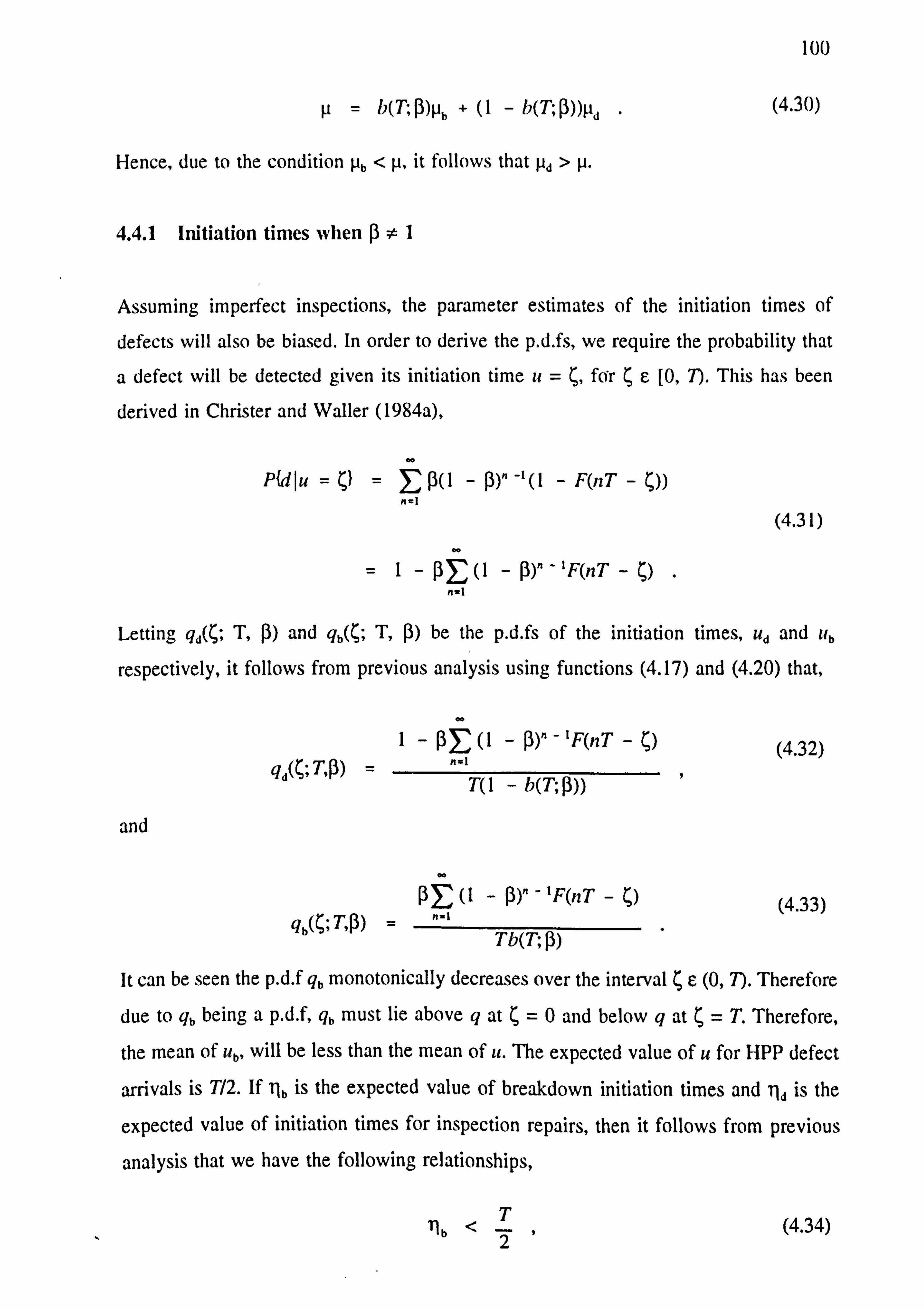
100

µ= b(T; ß)µb + (1 - b(T; ß))µd .

(4.30)

Hence, due to the condition Nb < µ, it follows that µd > µ.

4.4.1 Initiation times when ß#I

Assuming imperfect inspections, the parameter estimates of the initiation times of

defects will also be biased. In order to derive the p. d. fs, we require the probability that

a defect will be detected given its initiation time it for ýe [0, T). This has been

derived in Christer and Waller (1984a),

P{d Iu (1 - F(nT - ý))

(4.31)

=1-ß (1 - (3)" - `F(nT - ý) /ýs]

Letting qA; T, ß) and qA; T, (3) be the p. d. fs of the initiation times, Ud and Ub

respectively, it follows from previous analysis using functions (4.17) and (4.20) that,

1- OE (1 - ß)" - 'F(nT - ý) (4.32) 9d(ß: TO) _ "_'

T(1 - h(T; ß)) '

and

Týßý _ qA;

IF(nT - (4.33) n-1

Tb(T; 13)

It can be seen the p. d. f q, monotonically decreases over the interval ýe (0, T). Therefore

due to qb being a p. d. f, qb must lie above q at c=0 and below q at C=T. Therefore,

the mean of ub, will be less than the mean of it. The expected value of u for HPP defect

arrivals is T/2. If Ti,, is the expected value of breakdown initiation times and lid is the

expected value of initiation times for inspection repairs, then it follows from previous

analysis that we have the following relationships,

ý1 b<2 (4.34)

101

flbb(T; ß) + Td(1 -b(T; ß)) =T (4.35)

tad >T. (4.36)

We conclude that for both perfect and imperfect inspections, delay times and initiation

time parameter estimates will be biased given a censored data set. The delay times and

initiation times of defects repaired at inspection give rise to an overestimate of their

respective mean values. For the case of breakdown repairs, the delay time and initiation

time would provide an underestimate of their respective expected values. In practical

situations it may be necessary co collect censored data, and we now propose methods

to cope with a censored data set.

4.5 Correcting for Bias in Estimates of Delay Time and Initiation Time

Suppose that at least one of the following data sets of estimates have been obtained from

a field subjective data collection experiment, observing a total of, B say, breakdowns

and, D, inspection repairs of defects, namely,

Set {hb,; }, of failure based estimates of delay times, i=1,..., M,, where

M, <_ B, i. e the situation allows for not having captured all delay time

estimating opportunity available. It then follows the set {ub,; }, of failure

initiation times, corresponding to the i'th delay time, will also be

available.

2. Set {hd,; }, of inspection-repair based estimates of delay times, i=1,..., M2,

where M. S D, which implies not all inspection opportunities to estimate

the delay time are assumed taken. The set { 110) v of inspection-repair

initiation times estimates, corresponding to the i'th delay time estimate is likewise available.

102

The initiation times and times of failure are assumed to be measured from the start of

the inspection interval in which the defect or failure occurred. A prior p. d. f of delay

time, f(h, X) say, will be assumed available, where X is a set of parameters to be

estimated. Likewise, the defect arrival rate will be parameterised as g(u, y). The prior

format may be inferred from initial histogram plots of the data sets. A prior value of the

perfectness of inspection, (3, say, will also be assumed available.

4.5.1 Perfect Inspections, ßo = 1.

The p. d. fs of the initiation and delay times have been derived in Sections 4.2 and 4.4.

Hence, we can now formulate the likelihood for each data set:

M,

llfb(hbi; T, 2,. I) , (4.37)

M=

L2Q, ) _ rIfd(hdi; T, DIY) "

(4.38) ; _,

M,

L9 b(uW; T, X., 1) , (4.39)

3L Y=ý

and

M2

L4(k, y) - 4d(«d;; T, ý, y) (4.40) 1=ý

Due to the perfect inspection assumption, it will be assumed that the delay times of

breakdowns, {h,,; }, are all less than T.

Maximum likelihood estimation could be applied to each likelihood function and

parameter estimates can be compared. The maximum likelihood method proposed in

Christer and Redmond (1990), is based on combining the delay time likelihoods Lt and

L2. Indeed the initiation time likelihood functions, L3 and L4, could also be combined and

parameter estimation carried out. The joint likelihood of only observing the breakdown

data set (1), would not be the product of Ll and L3 due to the delay time and initiation

time of each breakdown being dependent. To derive the joint likelihood, we first

condition on c'b =ý say. The p. d. f of the delay time hb would then be f(4)/F(T - ý),

103

05ýST-ý. Hence, combining this p. d. f with the p. d. f of ub, function (4.16), it

follows after simplification that the joint likelihood of observing breakdown data set (1)

is given by,

L= IJ'1b.

t ý) 9(iýb. ý ýY) (4.41)

h , _1 b(T; X, 1)

Likewise the joint likelihood of observing the inspection repair delay time set (2) is

given by,

L_f f(ha.; ; 2) g(lld, 1 ; Y) (4.42)

ai1_ b(T, X, y)

It can be seen that when the p. d. f of u is assumed to be known, e. g uniform, the

likelihoods Lb and Ll are equivalent, in respect to estimation, after omitting the factors

q(u) and Q(u) respectively from each likelihood. Similarly, Ld and L. would be

equivalent for this case. This is expected due to selecting the prior distribution of u. If

data is available for both breakdowns and inspection repairs, then the combined

likelihood, i. e the product LbLd, can also be used to provide parameter estimates.

It is evident that a number of likelihoods could be used to obtain parameter estimates.

This is an advantage, because if we obtain similar maximum likelihood estimates from

different likelihood functions then greater confidence exists in modelling assumptions,

such as perfect inspections or it may be the assumption of HPP defect arrivals. If

parameter estimates differ sufficiently the assumptions will need to be revised. Another

estimation procedure could be to allow the inspection period T be a parameter to be

estimated in the maximum likelihood process. The estimated T, say r, should then be

approximately equal to T for the model assumptions to hold. However, a large amount

of data may be required for this test to work, due to the increased number of parameters

in the likelihood function.

It will now be shown that given an uncensored data set, i. e when Ml =B and M2 = D,

the maximum likelihood estimate of parameters for an initiation time and delay time

distribution will be unbiased (in the asymptotic sense. ) Assume B breakdowns have

arisen in one inspection interval (0,7) and D defects were repaired at the inspection.

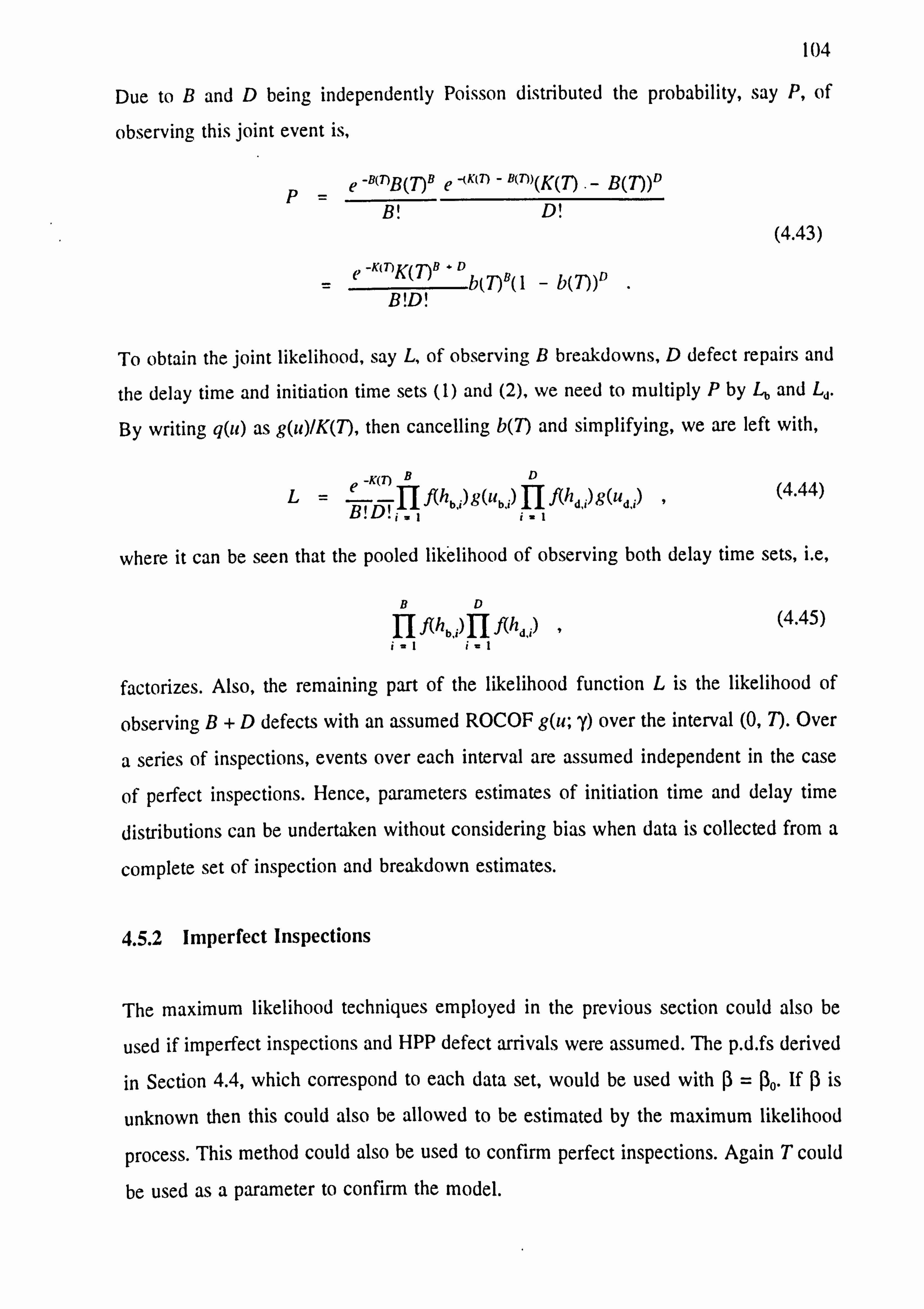
104

Due to B and D being independently Poisson distributed the probability, say P, of

observing this joint event is,

e -amB(T)B e -(K(n - e(7))(K(7) B(7))° B! D!

(4.43) K171 B "D

_c' K(T) b(7) (1 - b(7))ß

B! D!

To obtain the joint likelihood, say L, of observing B breakdowns, D defect repairs and

the delay time and initiation time sets (1) and (2), we need to multiply P by Lb and Ld.

By writing q(u) as g(u)/K(T), then cancelling b(T) and simplifying, we are left with,

e -Km B f(hb.

i)9 `(11b) f(

D ý/h

d i)g(ud. i) (4.44) L='

B! 5T i=ý I i= t

where it can be seen that the pooled likelihood of observing both delay time sets, i. e,

BD

II f(hb ) Il f(hd )" (4.45) i-1 i=1

factorizes. Also, the remaining part of the likelihood function L is the likelihood of

observing B+D defects with an assumed ROCOF g(u; y) over the interval (0,7). Over

a series of inspections, events over each interval are assumed independent in the case

of perfect inspections. Hence, parameters estimates of initiation time and delay time

distributions can be undertaken without considering bias when data is collected from a

complete set of inspection and breakdown estimates.

4.5.2 Imperfect Inspections

The maximum likelihood techniques employed in the previous section could also be

used if imperfect inspections and HPP defect arrivals were assumed. The p. d. fs derived

in Section 4.4, which correspond to each data set, would be used with ß= ßo. If 0 is

unknown then this could also be allowed to be estimated by the maximum likelihood

process. This method could also be used to confirm perfect inspections. Again T could

be used as a parameter to confirm the model.

105

4.6 Additional Tests of Model Fit

Splitting the delay time and initiation time data into disjoint sets based on failures and

inspection repairs can provide additional tests of fit to those given in Chapter 3, even

with uncensored data. The procedure can also help in verifying modelling assumptions.

Let the model parameter estimates be L', y') for perfect inspections with NHPP defect

arrivals or L', ß) for imperfect inspections with HPP defect arrivals. We could, for

example, then proceed with distribution tests such as K-S or chi-square on all or some

of the data sets of delay time and initiation, assuming enough data is available for each

case.

4.7 Conclusion

It has been seen that a statistical bias can exist in the data leading to parameter estimates

of delay time and initiation time for censored data. Breakdown based observations give

rise to an underestimate of delay time and initiation time, whilst observations based

upon defects identified and repaired at inspections give rise to overestimates. The bias

has been shown to be dependent on inspection frequency and the perfectness of

inspections.

Methods based on maximum likelihood have been proposed to correct for the bias have

been proposed, which leads to the estimation of the actual initiation time and the delay

time distributions.

In the case of censored data, it may be possible that parameters for the delay time

distribution can be estimated to an acceptable degree of accuracy by updating procedures

instead of performing the bias correction. Some form of iteration method could also be

adopted. The task of parameter fitting will be further investigated in the next chapter on

simulation.

106

Chapter 5

Simulation Study of the

Delay Time Model

5.1 Introduction

A simulation study is undertaken to further investigate and verify the delay time models

and proposed method of analysis of earlier chapters. Simulation programs, written in

Pascal, have been used to simulate the delay time process given sets of input parameters

and assumptions. Simulation algorithms are derived for the case of perfect inspections

and instantaneous repair of breakdowns. Then, these modelling assumptions are relaxed

to imperfect inspections and non-instantaneous breakdown repairs. The outputs of

simulation experiments are analyzed and compared to the appropriate theoretical values

of the models of the earlier chapters.

An investigation is undertaken into the accuracy and effectiveness of the parameter

estimation procedures given in Chapters 3 and 4. Correction of bias is carried out on

censored simulated data. The effects of not correcting for bias but using an updating

method, as a further option, is also explored. An iteration method is developed which

alternates between updating the scale parameter of a Weibull delay time distribution and

only estimating the shape parameter using maximum likelihood. The estimation of delay

time distribution parameters based upon only observational data (failure times and

number of defects detected at inspections) is also demonstrated. Results are shown for

simulated data sets and conclusions drawn.

107

5.2 Pilot Simulation of the Delay Time Model

A simulation of the delay time model would involve simulating over a time period for

a set of inspect; ons when defects would arise within each inspection interval. However.

for a pilot simulation, we shall assume one defect to arrive in one inspection interval,

say (0, T). This model along with its development could be used as a modelling module

6 in a more complex situation. The outcome for a defect, i. e failure or detected at inspection, can then be repeated for N defect trials. Given this assumption, we can then

calculate, for example, the proportion of failures arising for different values of T. which

should asymptotically agree with the model b(T), that is function (2.15), as the number

of simulated defect trials, N --4 °. We shall first deal with the perfect inspection case,

Section 2.5.1, and then with the imperfect inspection case.

5.2.1 Perfect Inspections

The following assumptions will initially be assumed to apply for the system to be

simulated:

(a) The conditional arrival time of a defect is uniformly distributed over the

interval (0, T) since the last inspection.

(b) The delay time of the defect is Weibull distributed with scale parameter

a and shape parameter y, the c. d. f being, F(h) =I- exp(-(cch)r). (c) Breakdowns are instantaneously repaired.

(d) The inspection at T is perfect. (e) The simulation will be repeated N times.

A program, DTS 1, written in Pascal, was used to perform this simulation. The method

used to generate random samples of is and It was the inverse transform method, see

Maisel and Gnugnoli (1972, p. 150), given a pseudo-random number generator which

generates uniformly distributed random numbers between (0,1). A seed value can also

be given to select different sequences of random numbers. The program requires as input

the input parameters ((x, 'y, T, N) and produces files containing the simulated events. The events recorded are u and It values for both failures and inspected defects.

108

The algorithm used to simulate the inspection process is as follows:

1. Generate the defect arrival time, u;, 1 <_ i <_ N, given by,

U=r. T (5.1)

where. r;, is a sequence of independent unordered uniform random

numbers on interval (0,1).

2. Generate the defect delay time, h;, for defect i, given by,

hl. =1 (-ln(9; ))"Y (5.2) a

where, q;, is another sequence of uniform random numbers.

3. Generate indicator variables, f, such that,

1 if u. + h, <T (5.3) f0 otherwise

where f=1 indicates the defect caused a breakdown and f=0 indicates

the defect was detected at the inspection T.

4. Tabulate results in files.

The program stores data in three files:

1. u;, h; and f, 1 <_ i <_ N (i. e all defect trials).

2. u;, h; when f=1, (failures only).

3. u;, h; when f=0, (detections only).

The user is informed of the total number of breakdown occurrences, BT say, given by,

N

Br=Ef, i=1

(5.4)

which will be binomially distributed with parameters N and b(T), where b(7) is the

probability a defect leads to a breakdown, given from equation (2.29) by,

109

T

b(T) =1-T fexp(-((xh)')dh (5.5)

h=0

The proportion of defects which have led to breakdowns, bT = ß, /N s:, y, having

expectation b(T), is also signalled.

The program was then extended to allow the user the option to investigate a series of

M equi-spaced inspection periods, T, 1 <_ j <_ M, resulting in a single file containing;

the inspection period, T, number of breakdowns, BTj, proportion of 'failures, bT;, and the

sample standard error, err; say, of bTJ, given by,

err, = bT(1 - b)I(N - 1) (5.6)

The sample standard error can then be used in constructing confidence intervals for the

proportion of defects arising as failures. For example, a run was carried out with the

following input parameters:

a=0.3, y=1.2, T= (2,4, ..., 20)' and N= 5000.

0.9 0.8 I-

-0 0.7

4) 0.6 0.5

0 0.4

-00.3 0 0.2

0.1 o+

0

Simulation

Model


Fig. 5.1. Comparison of a simulation run to the model for b(7).

A graph of the estimated proportion of breakdowns against the theoretical model (2.15)

of b(7), for the set of T values, is given in Fig. 5.1. The err, values lie between 0.004

and 0.007 indicating that a 95% confidence interval for the theoretical probability of a

breakdown {predicted to be b(7)) will have a width between 0.008 and 0.014. A

statistical test to compare the theoretical and sample proportions, b(7) and bT, was

carried out for all T values. The result was to accept the hypotheses that defects arise

as failures with probability b(T) for all T values under a 5% significance level.

0.3

0.25

0.2

c 0

o 0.15 CL 0 CL

0.1

0.05

0

Observations m Model

<1 23456789 10 Delay time class

Fig. 5.2. Histogram of breakdown delay time data versus theoretical model.

Members of the conditional delay time and initiation time sets {h;; f=1}, (h,; f. = 0),

{ u,; f" =1} and { u;; f=0} will be distributed with the p. d. fs of hb, hd, ub and if,,

respectively given by functions (4.5), (4.10), (4.18) and (4.20) respectively. In this way

the simulation process has been used to generate data to verify the theoretical

formulation of these p. d. fs. A comparison of the theoretical p. d. f and those generated

from the simulated results for delay times are given as an example in Figs. 5.2 and 5.3

when a=0.3, 'y = 1.2, T= 10 and N= 1000. In carrying out the chi-square goodness

of fit test, the test statistics for the two cases, namely breakdown and inspected delay

time, are 4.9 and 11.4 respectively. Adopting a 5% significance level, then. values

0.16

0.14

0.12

0.1 c 0 ö 0.08 OL

0- 0.06

0.04

0.02

0

Ee"


Fig. 5.3. Comparison of inspected delay time data versus theoretical model.

should be compared to x9 = 16.9 and x12 = 21.0 respectively. Clearly, the test statistic

are less in both cases. Hence, even if the physical evidence of Figs. 5.2 and 5.3 are not

accepted, given the additional significance, we accept the hypotheses that the delay time

simulation observations are distributed with p. d. fs (4.5) and (4.10) respectively.

5.2.2 Imperfect Inspections

Imperfect inspections can easily be dealt with by extending the previous method. Let (3

be the probability a defect is detected and repaired at an inspection, if it is present.

Assume also that the process of periodic inspections continues indefinitely, so that a

defect which arises in an interval (0, T), will eventually arise either as a breakdown or

be repaired at an inspection.

For a defect with arrival time, u;, and delay time, h;, 1 <_ i <_ N, the defect will cause a

failure if not detected within [(u; + h; )/TJ inspections which is an event with probability (1 -, where [x] denotes the integer part of x. Hence, if we redefine the

indicator variable, f;, so that it is given by,

<1 23456789 10 11 12>12 Delay time class

112

if r< < (1 - Not. + ti, )/71 (5.6)

f` 0 otherwise

where r; is uniform (0,1), it follows that f=1 implies the defect causes a breakdown

over the current inspection period or a future inspection period and f =O implies the

defect is repaired at an inspection.

A numerical example for b(T) is given in Fig. 5.4 when ß=0.7, a=0.3, 'y = 1.2 and

N= 1000 and T=2,4,..., 20. Close agreement between b(T) and simulation estimates

is attained. Members of the conditional delay time and initiation time sets {h;; f. =1},

{ h,; f= 0), { u;; f=1} and { u;; f=0} will be distributed with the p. d. fs of hb, hd, ! 1b

and Ud, respectively, given by functions (4.26), (4.29), (4.32) and (4.33). Numerical

examples for delay time are given in Figures 5.5 and 5.6 for T= 10. Close agreement

is achieved which again verifies the formulation of the p. d. fs formulated in earlier

chapters. In carrying out the chi-square goodness of fit test, the test statistics for the two

cases, namely breakdown and inspected delay time, are 12.2 and 6.6 respectively.

Adopting a 5% significance level, these values should be compared to XIO = 18.3.

Clearly, the test statistics are less in both cases. Hence, we accept the hypotheses that

the delay time simulation observations are distributed with p. d. fs (4.26) and (4.29)

respectively.

The simulation procedure is a module for the simulation of an inspection practice of a

system. The next section deals with the simulation of the delay time process over a

series of inspections taking into account downtime, cost and assuming defect arrivals

arise as a rate process over time.

113

0.9

F- -00.8 V

0.7

0.6

0.5 0 L- d

0.4

0.3-+ 0

Simulation

Model


Fig. 5.4. Comparison of imperfect inspection model b(T) with simulation.

0.25

0.2

c 0.15 0 L. 0 0 d 0.1

0.0 5

n <2 468 10 12 14 16 18 20 >20

Delay Time Class


Fig. 5.5. Imperfect inspection p. d. f of breakdown delay time versus simulation.

114

0.16

0.14

0.12

0.1 c 0 ö 0.08 CL 0 L.

0' 0.06

0.04

0.02


Fig. 5.6. Imperfect inspection model for inspected delay time versus simulation.

5.3 Simulation over a Series of Inspections

We give here a method to simulate the delay time process over a series of inspections.

First, perfect inspections with instantaneous breakdown repairs are dealt with. Then, we

relax these conditions to include the case of imperfect inspections and non-instantaneous

breakdown repairs.

5.3.1 Perfect Inspections

We assume the following assumptions apply to a situation to be simulated over a series

of inspections:

(a) The system is defect free at the start of simulation.

(b) N perfect inspections will be undertaken with period T.

(c) Defects arise as a homogeneous Poisson process (HPP) with rate parameter k

<2 468 10 12 14 16 18 20 >20 Delay Time Class

115

over each of the N inspection intervals.

(d) The delay time of each defect is Weibull distributed with scale parameter a and

shape parameter y.

(e) Breakdowns are instantaneously repaired.

It is clear that the number of defects to arrive in each inspection interval (0,7) is Poisson

distributed with mean U. Hence, one approach to simulating the system could be to

generate samples from the Poisson distribution for the number of defects to arrive in

each of the N inspection intervals and then use the pilot simulation method for each

inspection. There are many methods to generate Poisson samples. One method, which

was the method adopted, is to use the result that the time between defect arrivals is

exponentially distributed with mean 1/k. If r; is a sequence of uniform (0,1) random

numbers then,

e. _-! ln(r) (5.7)

is a sequence of exponentially distributed random variables of mean 1/k. Consider the

number of defects, A say, to arrive in an inspection interval. For A to be Poisson

distributed with mean kT we need to sum the values e; until the result exceeds T. Hence,

let un say, be the n'th summation, given by,

un = Fe, , uo = 0, n=1,2... (5.8)

. =t

Then let A be given by,

A= {n; it, <_ T, itn, l > (5.9)

It follows that A is Poisson distributed with the required mean value. The pilot

simulation method can then be used to calculate the number of breakdowns arriving over

the interval (0, T). However, for the case of HPP defect arrivals the generation of A has

also generated a sample of defect arrival times, i. e the set { u"), 1 <_ it <_ A, for A>0.

Essentially, this set is the order statistics of a set of A independent uniform random

samples on the interval (0,7).

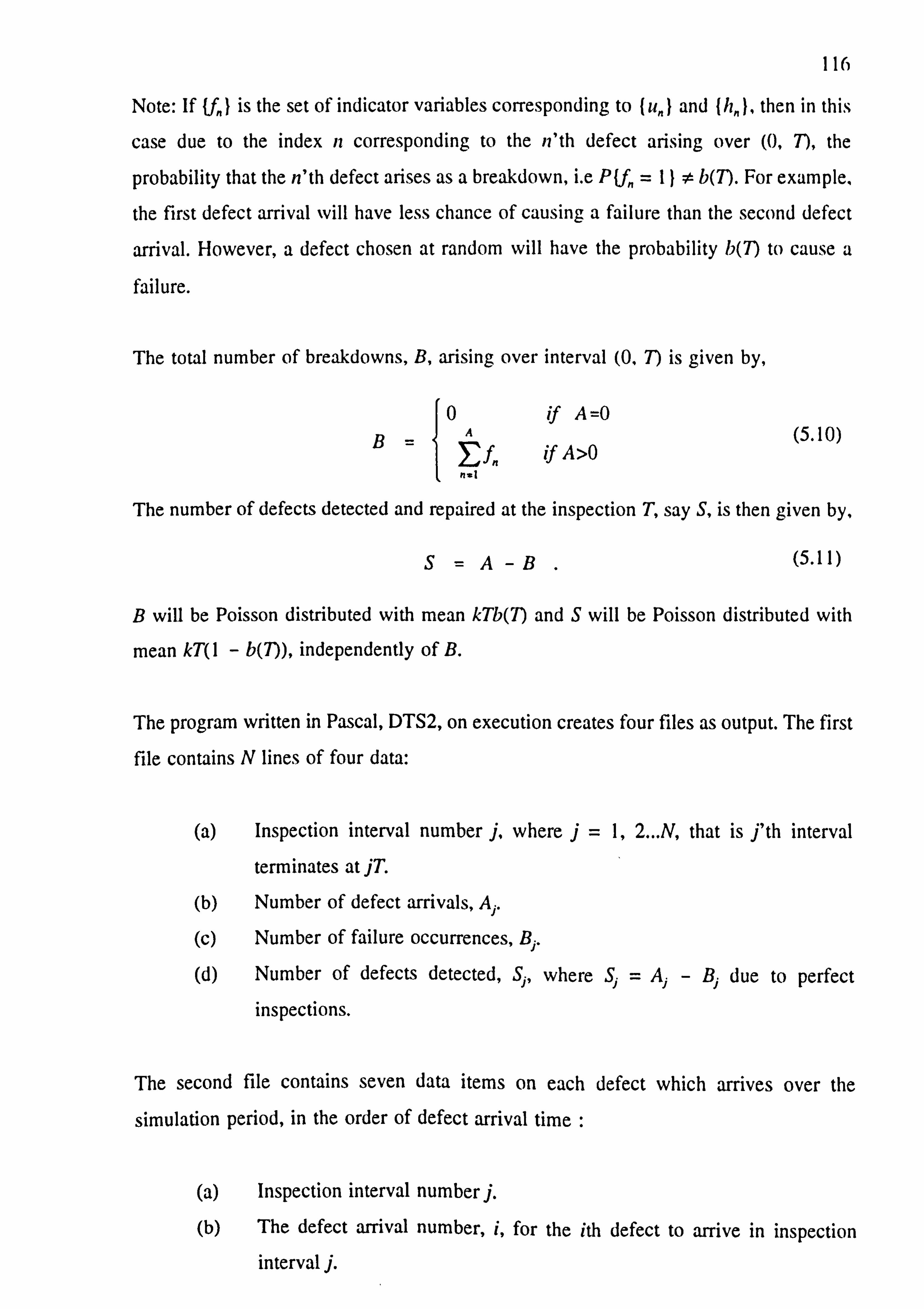
116

Note: If If, } is the set of indicator variables corresponding to (u,, } and {Ii}. then in this

case due to the index n corresponding to the n'th defect arising over (0, T), the

probability that the n'th defect arises as a breakdown, i. e P{fn =I}# b(T). For example,

the first defect arrival will have less chance of causing a failure than the second defect

arrival. However, a defect chosen at random will have the probability b(7) to cause a

failure.

The total number of breakdowns, B, arising over interval (0, T) is given by,

10 if A =0 B=A (5.10) fn if A>0

n: l

The number of defects detected and repaired at the inspection T, say S, is then given by,

S=A -B . (5.11)

B will be Poisson distributed with mean kTb(T) and S will be Poisson distributed with

mean kT(1 - b(T)), independently of B.

The program written in Pascal, DTS2, on execution creates four files as output. The first

file contains N lines of four data:

(a) Inspection interval number j, where j=1,2... N, that is j'th interval

terminates at jT.

(b) Number of defect arrivals, Aj.

(c) Number of failure occurrences, B1.

(d) Number of defects detected, S1, where S, = Aj - B1 due to perfect inspections.

The second file contains seven data items on each defect which arrives over the

simulation period, in the order of defect arrival time :

(a) Inspection interval number j.

(b) The defect arrival number, i, for the ith defect to arrive in inspection

interval j.

117

(c) Delay time of defect, h.

(d) Arrival time of defect, u, from start of inspection interval j.

(e) An indicator variable, f, where f=0 if defect was detected,

(i. e. if it +h> T), and f=I if defect caused a failure (i. e if it +h <_ T).

(f) How long ago defect first arrived. HLA, where HLA =T- it, if f=0, and

HLA=h. iff=I.

(g) How much longer, HML, the defect can be left before causing a failure

where, HML = 0, if a failure, and HML = it +h-T, if inspected.

The third file contains only the data on defects which were inspected. The items of data

will be the same for the defect file except for the indicator variable, f. The fourth file

contains only the data on defects which caused a failure. The items of data are (a), (b),

(c) and (d) from the first file plus the following :

(a) The time of failure, yb, where Yb =u+h. The p. d. f of yb is given by

function (3.34).

(b) The failure arrival number, in, for the m'th failure in inspection interval

J.

The following parameter values have been selected for an initial test,

k=0.5, a=0.2, "y= 1.2, T= 10, N= 1000.

The theoretical mean and standard deviation of the sampled variables are tabulated in

Table 5.1, along with the sample mean, standard deviation and standard error of mean

from a simulation run. Some variables have a suffix implying a condition; b indicates

breakdowns and d indicates detections. The total number of defects arising for this

particular test was 4918 with 2823 failures. It can be seen that there is close agreement

between theoretical parameters and sample estimates, validating the simulation

procedure.

5.3.2 Imperfect inspections

A program, DTS3, was written to accommodate imperfect inspections. The probability,

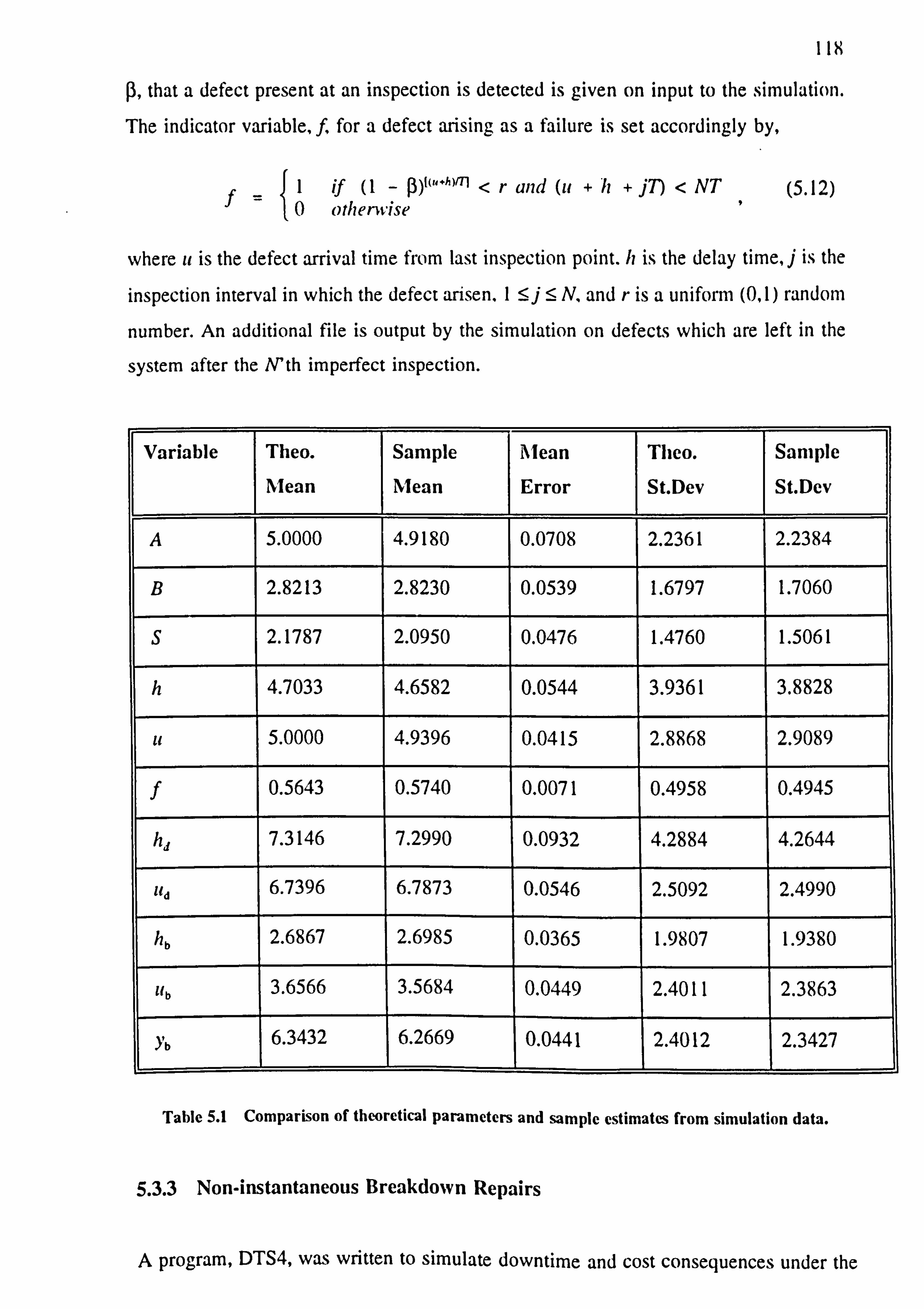
118

P, that a defect present at an inspection is detected is given on input to the simulation.

The indicator variable, f, for a defect arising as a failure is set accordingly by,

f_1 if (1 - p)E(t4 )m <r and (it + ii + JT) < NT (5.12) 0 otherwise

where it is the defect arrival time from last inspection point. h is the delay time, j is the

inspection interval in which the defect arisen. 1 <_ j: 5 N, and r is a uniform (0,1) random

number. An additional file is output by the simulation on defects which are left in the

system after the Nth imperfect inspection.

Variable Theo.

Mean

Sample

Mean

Mean

Error

Theo.

St. Dev

Sample

St. Dev

A 5.0000 4.9180 0.0708 2.2361 2.2384

B 2.8213 2.8230 0.0539 1.6797 1.7060

S 2.1787 2.0950 0.0476 1.4760 1.5061

h 4.7033 4.6582 0.0544 3.9361 3.8828

it 5.0000 4.9396 0.0415 2.8868 2.9089

f 0.5643 0.5740 0.0071 0.4958 0.4945

h, j 7.3146 7.2990 0.0932 4.2884 4.2644

tcd 6.7396 6.7873 0.0546 2.5092 2.4990

hb 2.6867 2.6985 0.0365 1.9807 1.9380

ub 3.6566 3.5684 0.0449 2.4011 2.3863

yb 6.3432 6.2669 0.0441 2.4012 2.3427

Table 5.1 Comparison of theoretical parameters and sample estimates from simulation data.

5.3.3 Non-instantaneous Breakdown Repairs

A program, DTS4, was written to simulate downtime and cost consequences under the

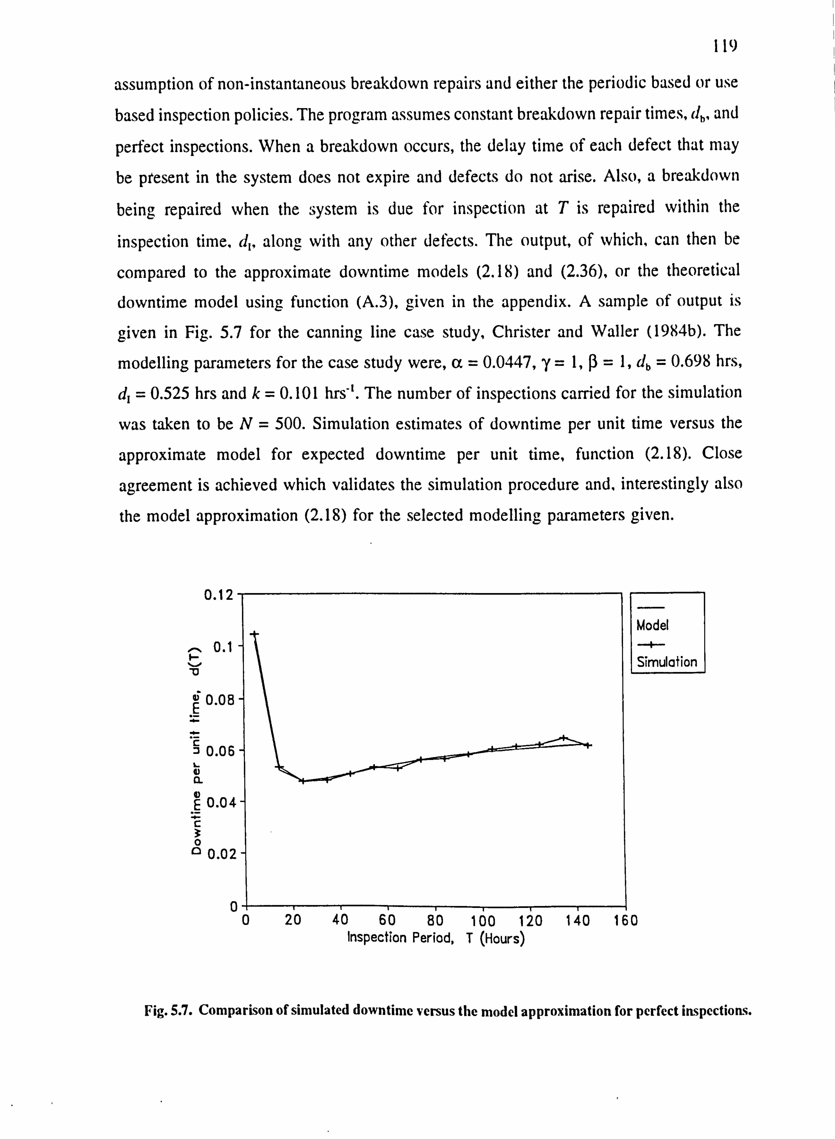
119

assumption of non-instantaneous breakdown repairs and either the periodic based or use

based inspection policies. The program assumes constant breakdown repair times, db, and

perfect inspections. When a breakdown occurs, the delay time of each defect that may

be present in the system does not expire and defects do not arise. Also, a breakdown

being repaired when the system is due for inspection at T is repaired within the

inspection time, d,, along with any other defects. The output, of which, can then be

compared to the approximate downtime models (2.18) and (2.36), or the theoretical

downtime model using function (A. 3), given in the appendix. A sample of output is

given in Fig. 5.7 for the canning line case study, Christer and Waller (1984b). The

modelling parameters for the case study were, a=0.0447, y=1, (3 = 1, db = 0.698 hrs,

dI = 0.525 hrs and k=0.101 hrs. The number of inspections carried for the simulation

was taken to be N= 500. Simulation estimates of downtime per unit time versus the

approximate model for expected downtime per unit time, function (2.18). Close

agreement is achieved which validates the simulation procedure and, interestingly also

the model approximation (2.18) for the selected modelling parameters given.

0.12

,. 0.1

E 0.08

"ý 0.0 6

a E 0.04

C 3 0 ° 0.02

Model

Simulation

0 20 40 60 80 100 120 140 160 Inspection Period, T (Hours)

Fig. 5.7. Comparison of simulated downtime versus the model approximation for perfect inspections.

120

5.4 Estimation Techniques using Simulated Data

Chapters 3 and 4 have discussed various estimation techniques which can be applied to

a system given various sets of observational and subjective data. This section verifies

some of these methods and demonstrates other options available to the analyst.

5.4.1 Correcting for Bias in Delay Time Parameter Estimates

A program, MLEI, was written in fortran to verify the maximum likelihood procedure

given in Chapter 4, for the correction of bias due to the collection of delay times of

defects only at breakdowns or to the collection of delay times of defects detected only

at inspections. The program uses the likelihood functions Ll and L. given in Section 4.5.

A test was conducted using the following input parameters;

a=0.3, y=0.8, k=0.5, T= 10, N= 100,13= 1.

The theoretical probability of failure, equation (2.29) is, given the above parameters, b(T) = 0.673

.

Over the time period required for 100 simulated inspections, a total number of 485

defects had arisen, resulting in 310 failures and 175 inspected defects. The sample

estimate of the proportion of failures, that is the total number of breakdowns (310)

divided by the total number of defects (485), is,

b' = 0.638.

A 95% confidence interval for the theoretical probability of a breakdown is then given

by,

b* ± 1.97 0.638(1 - 0.638)/485 - (0.595,0.681) 9 (5.13)

which contains the theoretical value. After 100 inspections were performed, the histogram of delay times for the two cases are given in Figures 5.8 and 5.9, which also

compares the results with. the theoretical expectation.

The bias corrected estimates, for the set of the delay times of inspected defects and

121 breakdowns. {hd} and {hb} respectively, using equations (4.10) and (4.5) in the program

MLEI, were,

{ hd }: d=0.368,7 = 0.748, bA(T) = 0.683 and

{ hn }: a^ = 0.306, y^ = 0.796, b^(T) = 0.677,

where b"(7) is the estimated probability that a defect arises as a breakdown, using

function (2.29), with the estimated parameters in both cases.

The estimated p. d. fs are also given in Figures 5.8 and 5.9. The chi-square test was

carried out on both sets of data assuming the data is distributed with the appropriate

estimated conditional p. d. f. In the case of inspected delay times x2 = 8.63, and for the

case of breakdown delay times, X2 = 5.3. Adopting a 5% significant level, we reject the

hypothesis if X2 > 16.9 (9 degrees of freedom) for the first case, and we reject if

x2 > 18.3 (10 degrees of freedom) for the second case. Clearly, we can accept the

estimated p. d. fs in both cases.

It can be seen that for the case of breakdowns, bA(T) lies within the confidence limits

(5.14) of the probability a defect arises a failure. No updating in this case would be

considered necessary. Although, possible updating could be explored for the case { hd }

whereby the estimate bA(7) does not lie within the confidence limits (5.14). However,

it can be seen that bA(T) for this case does lie close to the theoretical value for the

simulation, b(7).

The main point, here, is that actual delay time population parameters can be estimated

given censored data sets.

5.4.2 Updating Option

An investigation is carried out to estimate the Weibull parameters assuming no bias

exists. It will be found that the estimated model b"(7) will be either greater or less than

the observed value b', depending on using breakdown or detected delay times. It is then

possible to use the scale update method given in Section 3.5.1. The effects of

undertaking this approach will be discussed.

122

0.5

0.45

0.4

0.3 5

0.3

0.25 ä

0.2

0.15

0.1

0.05

0 123456789 10

Delay time class

M

Simulation

Theory

Estimate

Fig. 5.8. Simulated breakdown delay time sample p. d. f versus theoretical model.

0.2

0.18

0.16

0.14

0.12 LA-

0.1 ä

0.08

0.06

0.04

0.02

0 2468 10 12 14 16 18 20 >20

Delay Time Class

Simulation M Theory

Estimate

Fig. 5.9. Simulated inspected delay time p. d. f versus theoretical model.

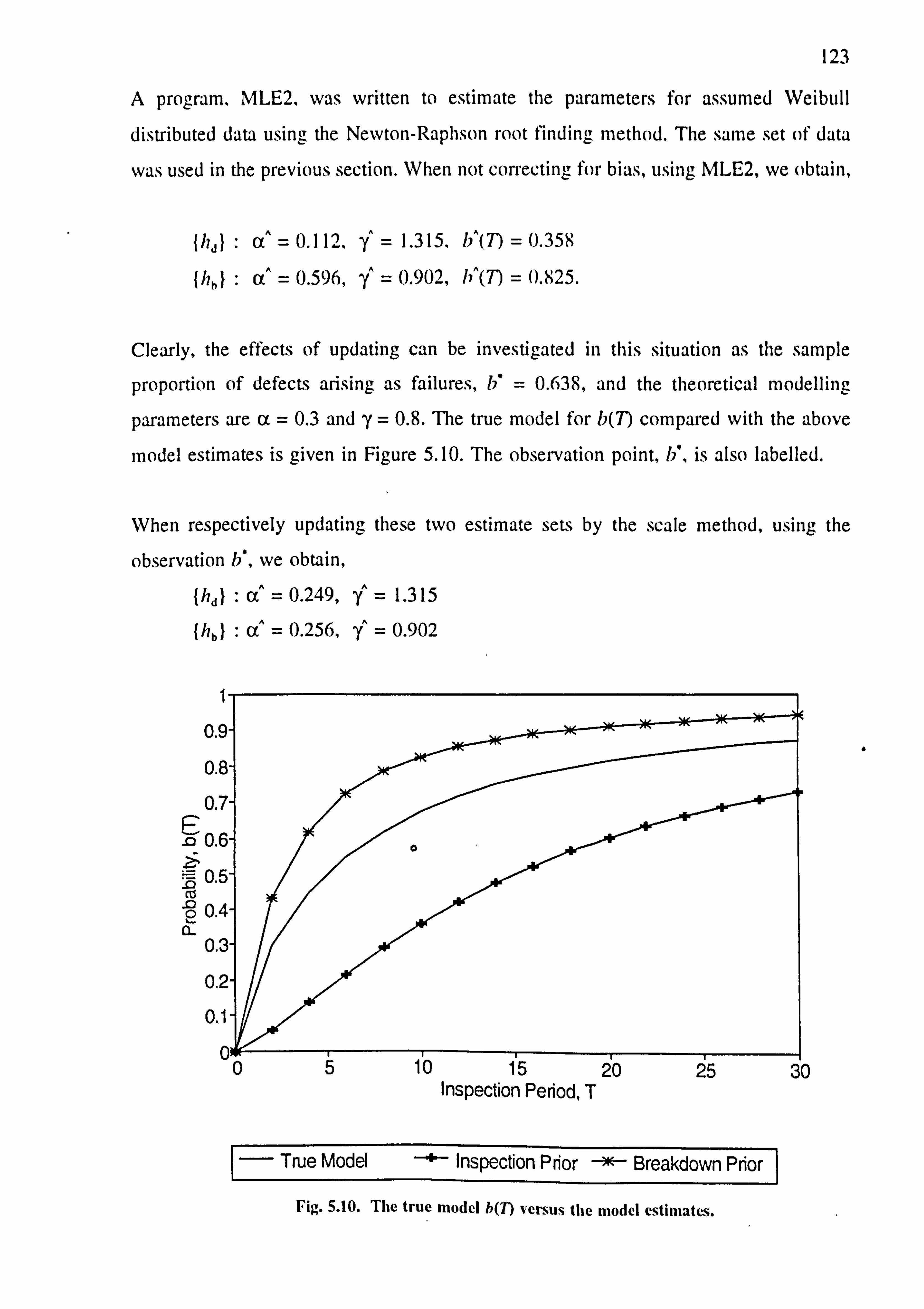
123

A program. MLE2, was written to estimate the parameters for assumed Weibull

distributed data using the Newton-Raphson root finding method. The same set of data

was used in the previous section. When not correcting for bias, using MLE2, we obtain,

{h, } : a% = 0A EI y=1.315, b"(, 7) = 0.358

{ hh }: d=0.596, y" = 0.902, hA(7l = 0.825.

Clearly, the effects of updating can be investigated in this situation as the sample

proportion of defects arising as failures, b' = 0.638, and the theoretical modelling

parameters are a=0.3 and 'y = 0.8. The true model for b(T) compared with the above

model estimates is given in Figure 5.10. The observation point, b', is also labelled.

When respectively updating these two estimate sets by the scale method, using the

observation b', we obtain,

{ hd a" = 0.249, y=1.315

{ hb }: a" = 0.256, y= 0.902

6

[Z

-0

Co .0 2 a

True Model -+- Inspection Prior -- Breakdown Prior

Fig. 5.10. The true model h(T) versus the model estimates.


124

It can be seen that, in both cases, there is improvement in the estimated scale parameter,

that is comparing it to the theoretical value of 0.3.

To investigate decision consequence of these estimating and updating procedures, the

model (2.23) of cost is used. The parameters selected were;

c, = 0.3 (cost of inspection),

c, = 0.5, (breakdown repair cost),

cd = 0.2 (defect repair cost) and

d, = 0.5 (inspection downtime).

The parameters were chosen so that the optimality conditions (2.25) and (2.26) are

satisfied. The theoretical optimum inspection period is,

7'=5.16,

and for the estimated models using the parameter estimates from updating, the optimums

are,

Inspection-Update : 7" = 4.35

Breakdown-Update :r=4.95.

Graphs of the true model versus the model estimates are given in Fig. 5.11. An error in

the optimum inspection period is about one time unit for the cost model based on the

inspected delay time defects. There is no significant error in the optimum inspection

period with the cost model based on breakdown repairs. As can be seen, both the cost

models based on the updating procedure, lie beneath the true model. In Section 5.4.4,

a test of model fit will be given to decide whether to accept the updated models.

5.4.3 Iteration Method to Capture Scale and Shape Parameters

A program, MLE3, was written to estimate the shape parameter of a Weibull distribution

given a set of delay time data observations and a value for the scale parameter. Perfect

inspections are assumed. Only minor modifications to MLE1 are necessary to perform

this. The re-estimated shape parameter is then used in the updating procedure to produce

an updated scale parameter. The procedures can be iterated until a possible convergence.

125

I- F- U a) E H

a) a U) 0 U -a a) U d)

W


True Model A Inspection-Update -*- Breakdown-Update

Fig. 5.11. The true cost model versus model estimates.

In both cases of the small data sample, convergence to 3 decimal places, occurs in 4

' iterations. The results obtained were,

Detected defects iteration : a" = 0.259, y% = 0.805,

Breakdown repairs iteration : a" = 0.260,0.789.

Close agreement between the estimated and input parameters ((x = 0.3, 'y = 0.8) has been

achieved through this process. In the case of a large data sample test (5000 defects in

all), using the simulation program DTS1 (Section 5.2.1) with a different set of input

parameters, even closer agreement was found between the estimated and input

parameters. The Weibull parameters selected for the delay time p. d. f of the large sample

case, were a=0.2 and '' = 1.2. The results obtained in 4 iterations were,

Breakdown repairs iteration : a" = 0.206, '% = 1.182

Detected defects iteration : a" = 0.206, y=1.185.

126

5.4.4 Criteria for Deciding on whether to accept the Updated Model

We have seen that a method exists for correcting the recognised bias in delay time

parameter estimates obtained from delay time measures captured at only breakdowns or

inspection situations. The first method (Section 5.4.2) based upon shearing the scale

parameter worked in one numerical case, based upon breakdown delay time estimates,

but didn't work in another, based upon inspection delay time estimates. The second

method (Section 5.4.3) based upon an iteration updating of both parameters gave

satisfactory results to both these numerical cases. What is now required is a means of

deciding whether or it necessary to update the estimates, and if so, what techniques to

adopt.

A simple method is proposed for deciding on whether to update via the bias correction

procedure or through use of the iteration method :

1. Perform a Chi-square test or K-S test on the censored delay times under

the hypothesis that the delay times are distributed by the conditional p. d. f

fb(ý; 7), equation (4.5) or fd(ý; T), equation (4.10) depending on breakdown-

based or inspection-based censoring.

2. If the test fails then either perform the bias correction method or the

iteration method. If the tests fail in these cases then the delay times may be assumed not to follow the Weibull distribution.

The Chi-Square values corresponding to each data set obtained by simulation in Section

5.4.1, when not correcting for bias and scale updating has been performed (Section

5.4.2), are as follows;

A { hd }: a=0.249, y=1.315, x2 = 150.2,

(hb) :d=0.256, Y% = 0.902, x2 = 9.94.

Using a 5% significance level, we reject the hypothesis if X2 > 18.3 for the first case (10

degrees of freedom), and reject if x2 > 16.9 for the second case (9 degrees of freedom).

127

Therefore, it follows that bias correction or iteration would not, on the basis of the test,

be necessary for the case of breakdown delay times. It is clear that bias correction or

iteration would be necessary for the detected delay times. Theses two conclusions agree

with, our previous analysis of the decision consequence for cost.

It is expected that when a decision not to correct for bias is taken, the models for cost

and downtime agree closely to the models when a correction is initiated. This is due to

the biased distribution and updated distribution being approximately equal.

Chi-square tests have been performed on the bias correction estimation and iteration

method. In all cases, these produce a decision not to reject the hypothesis.

An alternative procedure to test whether to correct for bias, would be to use the

observed times of breakdowns, if available. A K-S or Chi-Square test could be carried

out on the empirical sample of breakdown times measured from the last inspection. The

empirical distribution would then be compared to the theoretical distribution, function

(3.34), using the updated parameter set. The option is examined below.

5.4.5 Estimation using the observed breakdown times

The section verifies the maximum likelihood and method of moments procedures given

in Section 3.7, to estimate delay time parameters when the only data obtainable are

observations of breakdown times and the number of defects repaired at inspections. A

program MLE4, using equations (3.35), (3.36) and (3.41), was written to estimate the

Weibull delay time parameters, assuming perfect inspections (ß = 1) and given this type

of observational data.

A test was conducted given the input parameters; a=0.1, y=1.3, T= 30, N= 500 and

k=0.1. The total number of breakdown arrivals from this simulation were 1119 and the

total number of defects detected at inspections were 494. The maximum likelihood

parameter estimates of a and y, using the likelihood function (3.41), were a" = 0.100

and 'y = 1.24, which are acceptably close to the input parameters. Hence, it follows that

delay time modelling parameters can be estimated from only observations of breakdown

128

time and the number of inspection repairs.

We now turn to the method of moments method. The sample mean time of breakdowns

was 18.43. In solving the two equations for a and y. namely,

T

b(T. a,, y) 1(1

-e -"")dl= = 0.694 . (5.14)

hJa0

and

T

m(a, Y) =1 fh(1

-e -(("") dh =18.43, (5.15) Tb((x, y) ti=

the method of moment parameter estimates were a" = 0.100 and y=1.285. The

estimates are very close to the modelling parameters. Thus, the method provides an

alternative estimation procedure.

5.5 Conclusion

It has been seen that the simulation models and various parameter estimation procedures

produce results in agreement with theoretical models. This, validates the programming

of and the derivation of the delay time models and theory of the previous section. The

bias correction and iteration methods estimate the parameters of the delay time

distribution to within 10% of the theoretical values for a moderately sized sample, on

the tests carried out so far. The method of estimation using only observed data also

produces results in accordance with theory. We conclude that these are formal

techniques. However, convergence properties of the iteration method needs to be further

researched. The answer to the convergence will lie in the form of the log-likelihood

functions. E. g, for the case of failure delay times the log-likelihood function, omitting

constant terms due to assumed HPP defect arrivals, is given by,

F

L({hb}; (X, 'Y) = -F ln(b(T; a, y)) +E ln(f(h;; (x; y)) , (5.16)

i=1

where f is Weibull, F is the number of failures, b(7) is the probability of failure and {h; }

129

is the set of failure delay times, hb. The likelihood if not correcting for bias is the above

function without the Fln(b(T)) term. As the number of observations of hb increases, the

likelihood estimates when correcting for bias will be such that the estimated model b"(T)

will tend to b(T) the true model. Hence, the estimates can also be obtained by

conditionally selecting values of a and ? such that b(T) = b`, the observed proportion.

The maximum likelihood method under this condition is then the procedure to not

correct for bias. It is believed, for the work required here, that if convergence occurs

through the iteration method, then the estimates will tend to the maximum likelihood

estimates when correcting for bias, as the sample size increases.

Investigation into the error of the optimum inspection period when carrying out these

method also needs research. A clue could lie in the behaviour of the function b(T; a, 7)

for values of T, under the non-unique set ((x, y) which satisfy the observation point b'.

The cost and downtime curves under such restrictions, may have optimum inspection

periods which lie within a certain calculable interval. However, the measure of error, if

the iteration method gives accurate results in most cases, may not now be necessary to

consider.

The criteria for deciding whether to perform iteration or bias correction has produced

satisfactory results. The suggested decision procedures for deciding whether or not to

correct for bias may only work when the biased distribution can be approximated by a

Weibull distribution. This occurs in the test of Section 5.4.4, as the failures delay times

are almost exponential. A decision to not correct for bias may be made on the status-quo

point being satisfied. However, the resulting model for inspection periods other than the

current practice may be inaccurate. A further statistical test, such as, for example,

comparing the empirical and theoretical distribution of times of breakdowns, would need

to be applied.

Overall, simulation programs have been successfully written and tested, and methods

have been developed for estimating delay distributions given accurately estimated data

in practice. Further work could also lie in the effects of subjective errors when

estimating delay time, the possibility of imperfect inspections and convergence

properties of the iteration process.

130

Chapter 6

Application of Delay Time Analysis to

Concrete Structures

6.1 Introduction

This chapter gives an account of research supported by the Science and Engineering

Research Council (grant: GR/F/61196). The project was a collaborative venture between

operational researchers and civil engineers over 3 years. The main objectives were to

collect and publish data on the observed rates of deterioration of particular defect types

in a large number of concrete bridges and to develop predictive mathematical models

that relate inspection frequency to maintenance costs. The motivation was in part

associated with the prototype modelling paper for inspection practices of major concrete

structures, Christer (1988).

Concrete structures, like other civil engineering structures, deteriorate over their service

life. The main cause of this deterioration, in an adequately built structure, can be

described as environmental effects. Repair and maintenance represents an ever increasing

share of maintenance expenditure on concrete structures and there is, therefore, an

economic requirement to quantify and model the deterioration and maintenance process

of such structures. Repair options exist at different stages of deterioration with different

costs and consequences, and modelling is necessary to aid management decision making

to improve the cost effectiveness of maintenance expenditure.

A survey carried out by Queen Mary and Westfield College (QMWC) Concrete

Research Group, Rigden et al (1988), indicated that the principal cause of concern

amongst engineers with responsibility for structures was their inability to predict rates

of change of defective concrete components and to decide on the timing of concrete

131

repairs in order to make cost-effective decisions. Maintenance organisations were found

to be spending a great deal of time in analyzing and recording the conditions of

components. However, the data recorded was under-utilized, was subject to little by way

of analysis, and seldom led to any conclusions. It was not incorporated into any

predictive modelling.

There is evidently a need to develop and validate models of the random growth of

defects arising in components based upon data that is or could be collected. Christer

(1988) highlighted the scope for modelling deterioration and maintenance of concrete

structures, based on the concept of delay time, Christer and Waller (1984a), Baker and

Wang (1992), Baker and Christer (1994). RILEM (1988) gives an account of

engineering factors that may be necessary to include in a model for concrete deterioration and recognises that a component's life should be modelled at least as two

phases, namely defect free (initiation period) and defective (corrosive) period. The main

factors which affect the rate of degradation of reinforced concrete are assumed to be

environmental conditions, concrete type and concrete cover to the reinforcing steel, see

also Currie and Robery (1994).

The chapter reports on the delay time modelling of the growth of defects in concrete bridge components, the analysis of data collected and the development of cost based

inspection models. The two phase delay time model is extended to an extra phase in

order to model the process of cracking and spalling.

6.2 Deterioration of Concrete Components

Virtually every concrete structure eventually develops detectable cracks at some point in time of a sufficiently long service life. These may be already visible when built or

could develop and widen due to environmental factors such as corrosion of steel

reinforcement caused by the carbonation of the concrete or the impurities it may contain. If left to deteriorate, spalling will eventually occur, exposing the reinforcement and leading to corrosion, until the structure reaches a point in time when it is perhaps in an

unacceptable state for safety or other reasons and a major repair is deemed necessary. Defects deteriorate through a number of definable states where the time scale is

132

measured in years. Data analysis indicates that the time within a state is not

deterministic, and that the chance of changing state within a given period is dependent

upon the time duration within the current state, that is the deterioration is not

Markovian.

In the context of delay time. the time interval between the arrival of repairable cracks

and severe spalling would normally be the delay time measure, and repairs could be

undertaken at non-decreasing costs at any point over this interval of time. However, for

the present, the delay time will be split into two phases, namely cracking and spalling.

The key phases of the deterioration modelling are now, new to cracking, which occurs

at a time, u say, cracking to spalling which occurs over time, h, and spalling to failure

when repair is essential, which occurs after a further time period v. Defining a

component to be a section of a structure in which only one defect can arise, Fig. 6.1

depicts the deterioration over the cracking and spalling phases.

Defect free Phase Cracking Phase Spalling Phase

0U u+h u+h+v Defect Multiple Minor Spalling with Free (New) Cracks Spalling

exposed reinforcement

Fig. 6.1. The Deterioration Phases of a Concrete Component.

By dividing the time into respective key phases, the effects of alternative maintenance

strategies can be explored. It is noted that the time intervals, u, h and v for this

application would be in the order of years, which is in sharp contrast to hours and days

133

observed in the delay time modelling of a mechanical plant, Christer and Waller

(1984b). Currie and Robery (1994) model the time from new to cracking and spalling

via a chemical process model and estimate the time to cracking at around 25 years and

spalling at around 40 years under nominal environmental conditions. However, there was

no discussion of the variance of cracking and spalling times. This chapter proposes to

model the distribution of time to these states using the inspection records of components

that were subjected to varying environmental conditions in order to predict consequences

of maintenance and inspection decisions.

6.3. Data Collection and Analysis

Inspection records from London Underground Limited and British Rail of concrete

bridges were analyzed by the co-researchers at QMWC. The records contained

information of inspection reports of bridge structures which constitutes snapshots of

condition spanning more than fifty years in some cases. Data extracted from the records

were entered into a linked database organised into three tables concerned with the

location, the structure and the defect type. The categories for each table are given in

Table 6.1. A unique code is provided for each component which had developed a defect

in at least the hairline cracked state. This is then used in linking and querying the

database. The structure table contains data on the structure type (e. g an overbridge) and

the component type (e. g a flexural beam) which is a member of the structure. The defect

table contains data on a set of inspection reports on each defect of a member. Exposure

relates to environmental conditions experienced by the component measured on a scale

mild, moderate or severe, and could change over the period of inspections undertaken.

Urgency is a code relating to the original inspector's judgement on whether to carry out

repairs or not. The key fault/action code is a number (L. 12) relating to the degree of

cracking/spalling of the component or the form of maintenance to be carried out on the

component. Current practice is to initiate maintenance on the recommendation of

inspectors and engineers following inspection reports. The categories are given in Table

6.2. Fault conditions I to 9 are ordered by the research team to represent the perceived

stages of degradation. The worst state of the component is recorded.

Complete data on around 700 defect arrivals on 400 bridges are currently held within

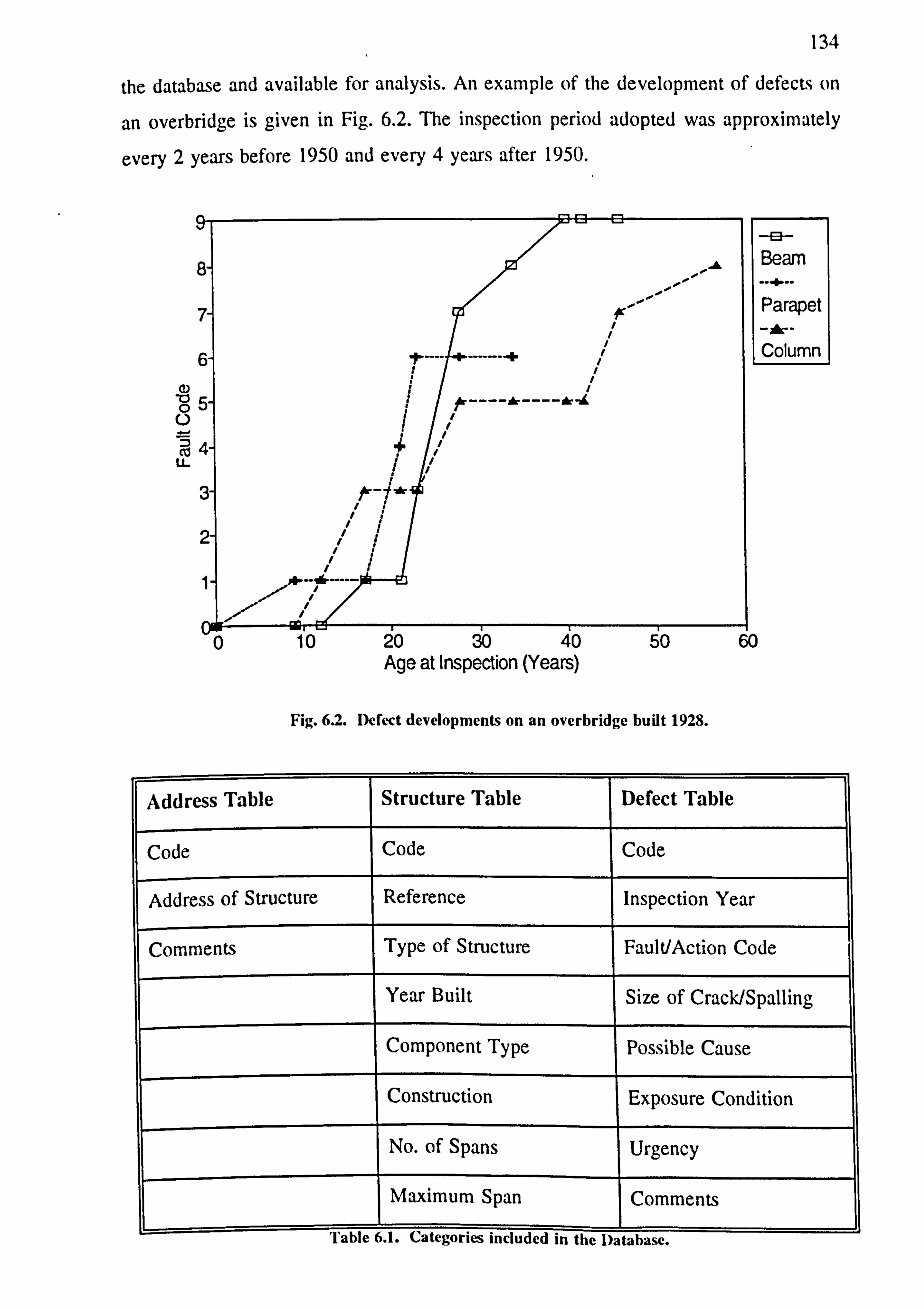
134

the database and available for analysis. An example of the development of defects on

an overbridge is given in Fig. 6.2. The inspection period adopted was approximately

every 2 years before 1950 and every 4 years after 1950.

(1) a 0 U

Co LL

A

--

I i i I I i i i

1* i i i i i i i1

U 1U 'LU ýlU 4U bU

Age at Inspection (Years)

Fig. 6.2. Defect developments on an overbridge built 1928.

E3 Beam

-+-- Parapet

-, -- Column

60

Address Table Structure Table Defect Table

Code Code Code

Address of Structure Reference Inspection Year

Comments Type of Structure Fault/Action Code

Year Built Size of Crack/Spalling

Component Type Possible Cause

Construction Exposure Condition

No. of Spans Urgency

Maximum Span Comments

1 aale o. i. categories Rncluaed in the Database.

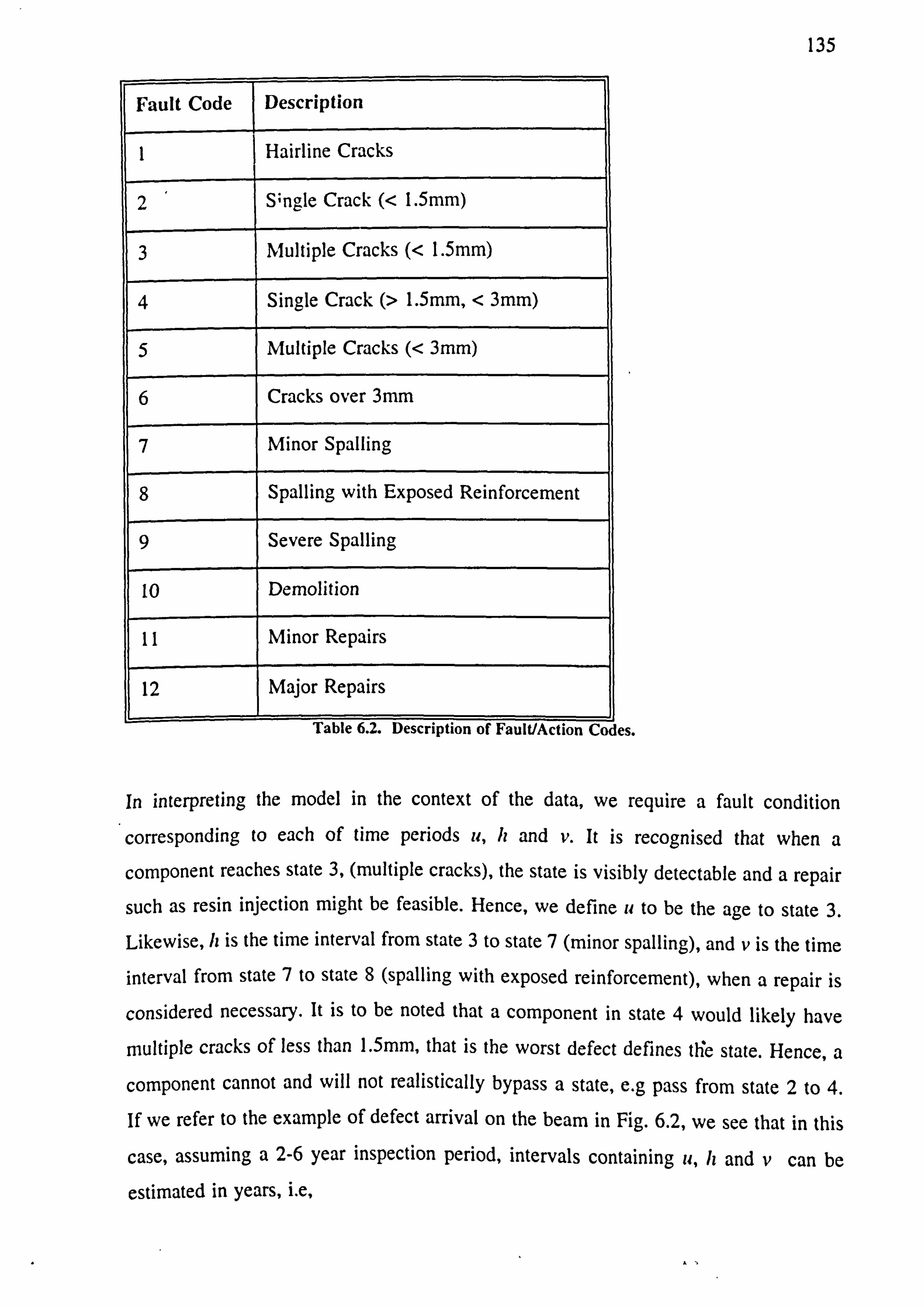
135

Fault Code Description

I Hairline Cracks

2 S; ngle Crack (< 1.5mm)

3 Multiple Cracks (< 1.5mm)

4 Single Crack (> 1.5mm, < 3mm)

5 Multiple Cracks (< 3mm)

6 Cracks over 3mm

7 Minor Spatting

8 Spatting with Exposed Reinforcement

9 Severe Spatting

10 Demolition

11 Minor Repairs

12 Major Repairs

table O. Z. Description of raultAction Codes.

In interpreting the model in the context of the data, we require a fault condition

corresponding to each of time periods u, h and v. It is recognised that when a

component reaches state 3, (multiple cracks), the state is visibly detectable and a repair

such as resin injection might be feasible. Hence, we define u to be the age to state 3.

Likewise, Iz is the time interval from state 3 to state 7 (minor spalling), and v is the time

interval from state 7 to state 8 (spalling with exposed reinforcement), when a repair is

considered necessary. It is to be noted that a component in state 4 would likely have

multiple cracks of less than 1.5mm, that is the worst defect defines the state. Hence, a

component cannot and will not realistically bypass a state, e. g pass from state 2 to 4.

If we refer to the example of defect arrival on the beam in Fig. 6.2, we see that in this

case, assuming a 2-6 year inspection period, intervals containing u, /i and v can be

estimated in years, i. e,

136

uc (21,23) uE (21,23) (6.1)

u+h c (23,28) h e- (0,7)

u+h+v c (28,34) ve (0,11)

The data clearly enables bounds upon the estimates of it, It and v to be established.

6.4. Modelling Deterioration of a Component

This section details the methodology used to model the deterioration of a concrete

component section subject to one defect arrival over time. Due to defects being recorded

only at inspections, a situation of censored data arises. One question which needs to be

answered, is whether the times u, h and v are mutually independent. Also, possible

dependency on exposure factors may need to be considered. Indications from an earlier

data sample show that defect developments within beams and columns share the same

p. d. f for u but not for values of It and v. This could be due to differing tensile forces

experienced across the element types. Aggressive exposure conditions have indicated an

increased rate of defect development which is as expected. As stated earlier, exposure

levels can vary over time. Hence, estimation of it, h and v will be undertaken without

conditioning on exposure levels, that is we assume exposure is a random factor in defect

development.

In the absence of strong indicators to the contrary, we assume the variables are mutually

independent and then proceed in deciding on a form or type of distribution for u, h and

v for a component type. This choice is aided by histograms of the lower and upper

estimates for the variables. Once distribution functions have been decided, maximum

likelihood estimation of the parameters of the selected p. d. fs can then be undertaken

based upon the interval data. For example, if we let g(u), ft h) and w(v) be the beam

component p. d. fs of u, h and v respectively, assuming independence between the phases,

then the contribution to the likelihood of the data for the defect arrival on the beam in

Fig. 6.2 would be :

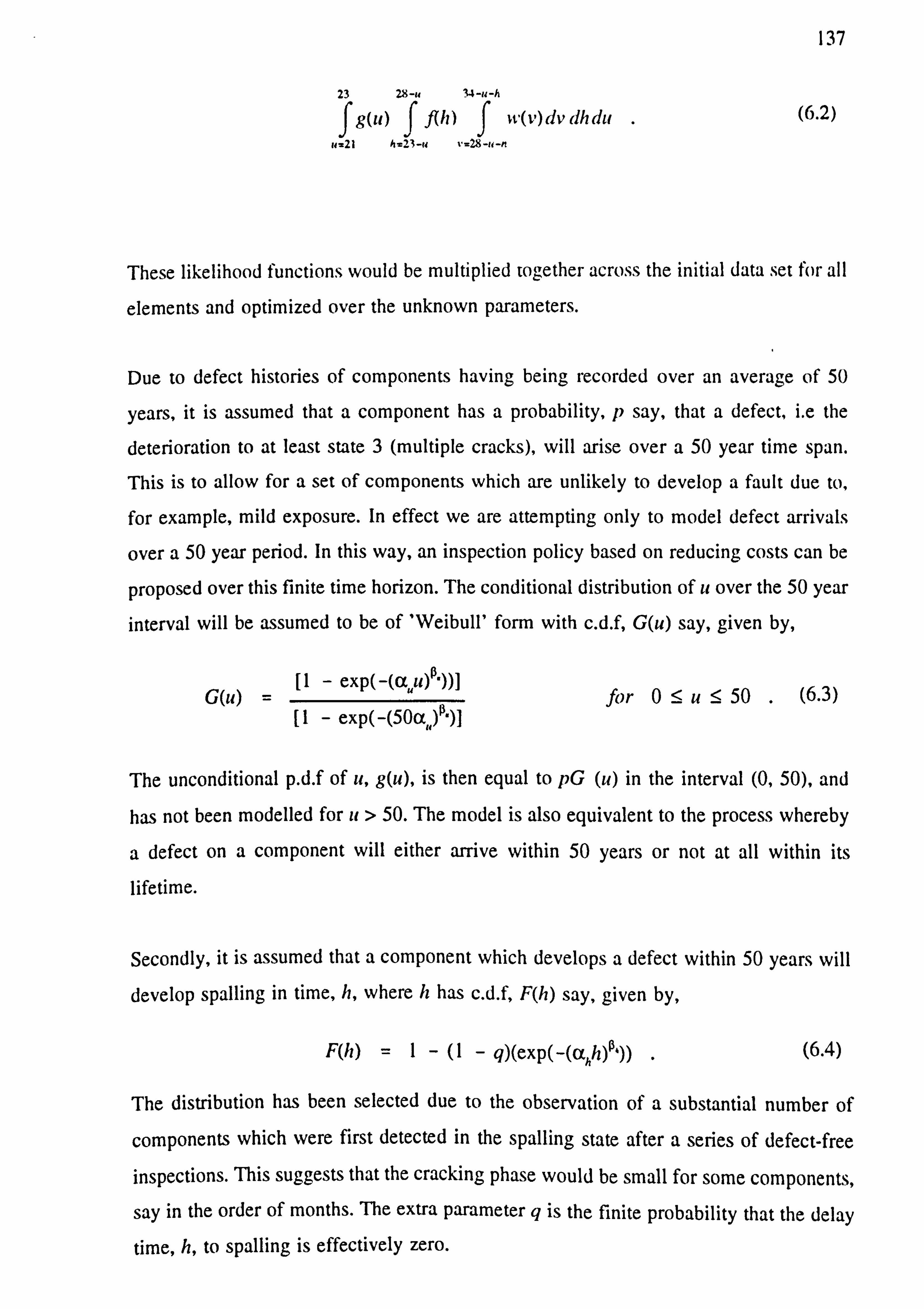
137

23 28-u 34-u-h f

g(u) f f(h) f

rt'(v)dvdhdu (6.2)

u: 21 h=23-u v=2$-u-n

These likelihood functions would be multiplied together across the initial data set for all

elements and optimized over the unknown parameters.

Due to defect histories of components having being recorded over an average of 50

years, it is assumed that a component has a probability, p say, that a defect, i. e the

deterioration to at least state 3 (multiple cracks), will arise over a 50 year time span.

This is to allow for a set of components which are unlikely to develop a fault due to,

for example, mild exposure. In effect we are attempting only to model defect arrivals

over a 50 year period. In this way, an inspection policy based on reducing costs can be

proposed over this finite time horizon. The conditional distribution of it over the 50 year

interval will be assumed to be of 'Weibull' form with c. d. f, G(u) say, given by,

G(u) = [1 - exp(-(auu)'-))]

[1 - exp(-(50(x«)a")] for 0<_u_<50 .

(6.3)

The unconditional p. d. f of u, g(u), is then equal to pG (u) in the interval (0,50), and

has not been modelled for it > 50. The model is also equivalent to the process whereby

a defect on a component will either arrive within 50 years or not at all within its

lifetime.

Secondly, it is assumed that a component which develops a defect within 50 years will

develop spalling in time, h, where h has c. d. f, F(h) say, given by,

F(h) =1- (1 - q)(exp(-((xhh)ß')) . (6.4)

The distribution has been selected due to the observation of a substantial number of

components which were first detected in the spalling state after a series of defect-free

inspections. This suggests that the cracking phase would be small for some components,

say in the order of months. The extra parameter q is the finite probability that the delay

time, h, to spalling is effectively zero.

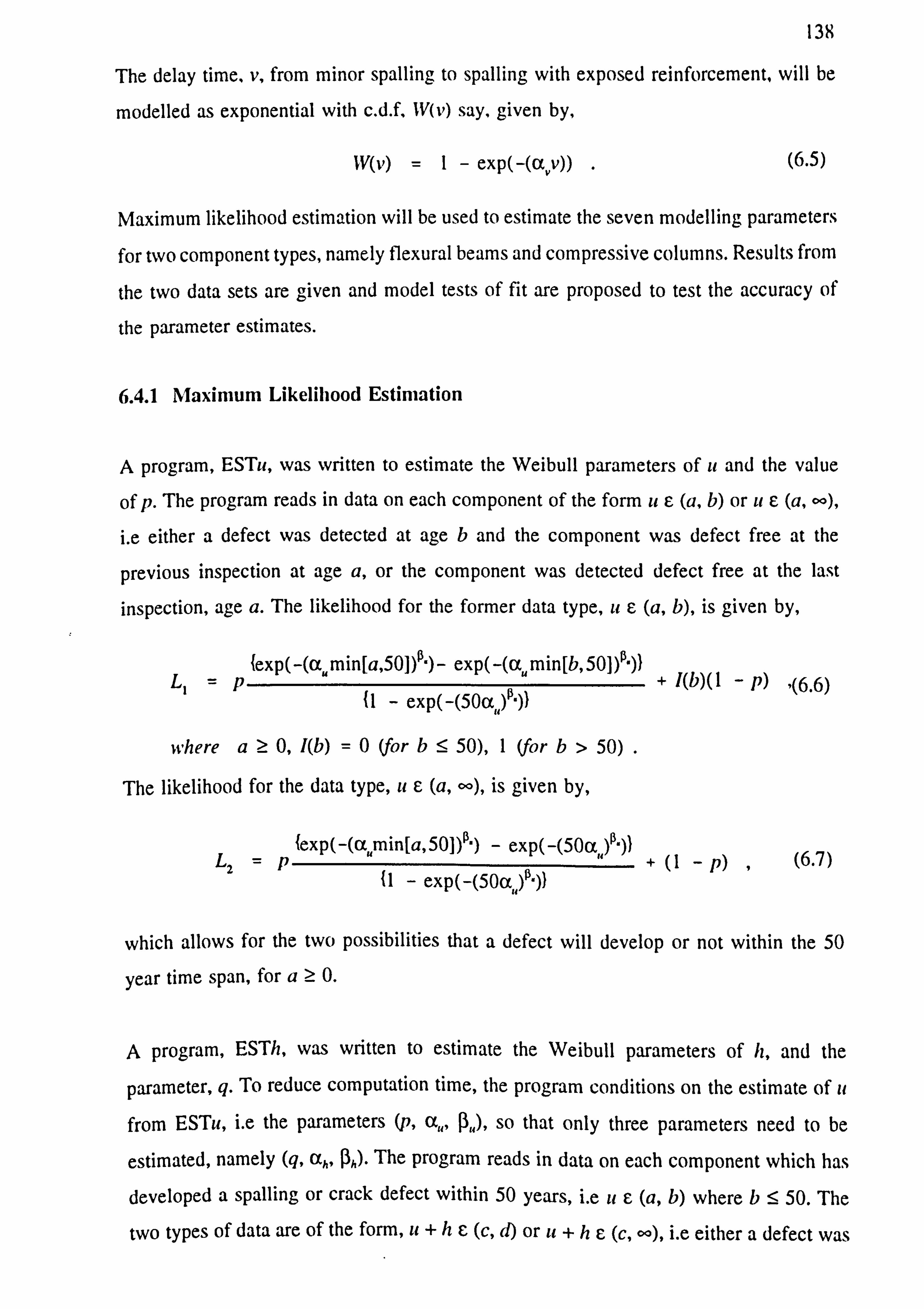
139

The delay time, v, from minor spalling to spalling with exposed reinforcement, will be

modelled as exponential with c. d. f, W(v) say, given by,

WV(v) =1- exp(-(avv))

Maximum likelihood estimation will be used to estimate the seven modelling parameters

for two component types, namely flexural beams and compressive columns. Results from

the two data sets are given and model tests of fit are proposed to test the accuracy of

the parameter estimates.

6.4.1 Maximum Likelihood Estimation

A program, ESTu, was written to estimate the Weibull parameters of it and the value

of p. The program reads in data on each component of the form is e (a, b) or it c (a, ('0),

i. e either a defect was detected at age b and the component was defect free at the

previous inspection at age a, or the component was detected defect free at the last

inspection, age a. The likelihood for the former data type, it e (a, b), is given by,

{exp(-(anmin[a, 50])a")- exp(-(ccU min [b, 50])0-))

{1 - exp(-(50a�)p"))

where a? 0,1(b) =0 (for b <_ 50), 1 (for b> 50) .

(6.5)

The likelihood for the data type, it e (a, oo), is given by,

L2 =p {exp(-(aumin[a, 5O])a") - exp(-(50(x,

4)ß")) +(1 -n) (6.7) {1 - exp(-(50a�)a")}

which allows for the two possibilities that a defect will develop or not within the 50

year time span, for a >_ 0.

A program, ESTh, was written to estimate the Weibull parameters of h, and the

parameter, q. To reduce computation time, the program conditions on the estimate of u

from ESTu, i. e the parameters (p, a,,, (3�), so that only three parameters need to be

estimated, namely (q, ah, P j. The program reads in data on each component which has

developed a spalling or crack defect within 50 years, i. e it e (a, b) where b <_ 50. The

two types of data are of the form, it + It e (c, d) or is +hC (c, co), i. e either a defect was

139

detected as a spall at age d and the component was cracked (or defect free) at the

previous inspection c, or the component was detected cracked at the last inspection, age

c. The likelihood for the first data type is given by,

b

LA = /' f G'(u)(F(d - ii) - F(c - u))dcu ,

(6.8) I. vO

and the likelihood of the second data type is given by,

b

L4 =pf Ga(u){1 - F(c - u)}dcc . (6.9)

u-a

A program, ESTuh, was also written to estimate the parameters of lt and h without

conditioning on u. The parameters obtained using this method produced exactly the same

parameter estimates obtained in ESTu and ESTh.

A program ESTv was written to estimate the v phase. Again, and to reduce computation

time, the program reads in the parameters (cc., ß,,, q, (Xti, ph) estimated from the programs

ESTu, ESTh and ESTuh. Therefore, only the parameter, av, needs to be estimated. The

program reads in data on each component which has developed a failure or spalling

defect and u is known to be less than 50 years. The two types of data are of the

form, u+h+ve (e, oo) or it +h+ve (e, J), i. e either a defect was last detected as a

spall (not severe) at age e or the component was detected failed at age f. The likelihood

for the first data type is given by,

bd

L5 =p 5GI(u)[(1

- WV(e - u))I(b, d) +f F'(h)(1 - Me-u-h))dh

J du

Im s tiac-� (6.10)

where l(b, d) =0 (for b# d), 1 (for b= d)

The likelihood for the second data type is given by,

bd

L6 =pf GI(u) q(W(e - cc) - W(f - u))I(b, d) +f F'(h)(W(e-u-h) - W(f-u-h))dh (it u=a h=c-u

(6.11)

140

6.4.2 Estimation on real data

A maximum likelihood calculation was undertaken on data from 195 beam components

and 176 column components using the programs ESTu, ESTh and ESTv. A check was

also made using the program ESTuh. The same parameter estimates for u and h were

obtained with this procedure. The results are given in Table 6.3.

Parameter Beams

195

Simulation

(200) (500)

Columns

176

Simulation

(200) (500)

p 0.665 (0.640) (0.676) 0.472 (0.445) (0.482)

au 0.035 (0.035) (0.036) 0.030 (0.024) (0.029)

2.08 (1.89) (2.08) 1.90 (1.63) (2.10)

q 0.472 (0.446) (0.434) 0.379 (0.382) (0.356)

ah 0.036 (0.033) (0.036) 0.022 (0.022) (0.024)

Ph 1.04 (1.02) (1.01) 2.11 (2.16) (2.06)

av 0.105 (0.135) (0.110) 0.033 (0.033) (0.033)

E(ul u< 50) (Years) 24.2 (23.3) (23.7) 25.3 (26.2) (26.8)

E(h) (Years) 14.3 (16.9) (15.8) 24.6 (24.9) (24.3)

E(v) (Years) 9.5 (7.4) (9.1) 30.3 (30.3) (30.3)

jLauic u. 3. rarameLer estimate results [or beams and columns.

A simulation was undertaken to test the proposed method. Parameter estimates for the beam and column components in Table 6.3 were selected as the theoretical parameters

of the simulation. A sample of 200 and 500 components were simulated with an inspection period of 2 years over a 50 year time span. The parameter estimates results

are given in brackets in Table 6.3. For the case of beam components, the estimated

mean values of u, h and v can be seen to converge to the input parameters. For the case

of column components, slight divergence in the mean of u for the larger sample can be

seen. However, the individual estimated parameters of u are closer to the input

141

parameters.

The main point, here, is that it is possible to obtain estimates of the distribution

functions of discrete snapshots in the concrete degradation process obtained from

available interval and censored data. It then remains to test the fit of the distribution and

to model the consequences of maintenance actions.

6.4.3 Test of Model Fit

Due to the censored nature of the data, a test of model fit was developed so as to

accommodate the interval type data. This test involves the Kaplan-Meier (K-M) estimate

of the reliability function for progressively censored samples, see Kalbfleisch and

Prentice (1980). Two K-M estimates are plotted by taking the uncensored observations

of u, first at u=A, and then at u=B, for the interval constrained event, ue (A, B). Due

to discrete observations of u, the K-M estimator, a nonparameteric representation, R'(u)

say, of the reliability function, R(u) =1- pG(u), is given by,

R "(u) _I1_d (6.12) j: u, <u n

where { u; }, is the sample of uncensored u values, d, is the number of coincidental

defective components at inspection time uS,, and nn is the number of defect free

components at time uu. The distribution of the K-M estimator is approximately normal.

The approximate variance of R'(u), V(u) say, is given by,

V ̀ (u) =R '(u)2 Ed (6.13) j: u, <u n(ný - d)

The variance can then be used to construct a 95% confidence interval (C-I) estimate for

the reliability function of u, R(u), that is R'(u) ± 1.96'[ß'(u), for u <_ 50. The maximum likelihood reliability estimate can then be tested for accuracy by seeing if it lies within the estimated confidence bounds over the 50 year range. Similar procedures apply to

time to spalling, u+h, and times to spalling with exposed reinforcement, at u+h+v.

142

Plots for beams and columns are given in Figures 6.3 - 6.8. The maximum likelihood

reliability fits, formulated using functions (6.3), (6.4) and (6.5), are plotted along with

the upper and lower K-M estimates, and the lower (upper) C-I bound for the lower

(upper) K-M estimate. The estimated C-I interval plotted would then be expected to be

slightly overestimated due to the interval constrained data. It can be seen that close fits

between the K-M estimate and the maximum likelihood estimate are achieved for both

beams and columns for u and u+h over 50 years, and u+h+v over 35 years for

beams and 50 years for columns. The lower and upper K-M estimators can be seen to

differ by approximately 4 years. This is due to the inspection period being

approximately 4 years. There are also crossovers between the two K-M estimators in the

plots for time to failure, Figs. 6.7 and 6.8. This is believed to be due to the small sample

size of detected failures. The maximum likelihood fits in all cases lie within the

confidence bands of the reliability function. Hence, given the additional confidence, we

accept the estimated model for concrete degradation. Interestingly, the hazard function

for u for both beams and columns is not strictly increasing over the range (0,50) years.

The hazard has a convex shape with a peak at around the conditional mean value of u.

This implies that a beam remaining in the defect free state for around 25 years is

unlikely to develop a defect over a 50 year span, say due perhaps to mild environmental

conditions or denser concrete.

For a test of independence between phases u and h, the sub-sample of components

where spalling was detected was selected. The mid-point of the interval of u, say um =

(a+ b)/2 was selected as a point estimate of u. Given this value of u, the value of h

would occur in interval (c - uo,, d- um). The mid-point of this interval was then selected

as an estimate of h. For a test of independence between phases h and v, the sub-sample

of components where spalling with exposed reinforcement was detected was selected.

The mid-point of the interval of u+h, say sm = (c + d)/2 was selected as a point

estimate of u+h. Given this value of u+h, the value of v would occur in interval (e -

sm, f- sm). The mid-point of this interval was then selected as an estimate of v. The

scatter plots for both cases are given in Figs. 6.9 and 6.10, and clearly indicate

independence between states.

143

cd co

0

a

---- Lower K-M Max. likelihood fit ----- Lower C-I Upper K-M ° Upper C-I

Fig. 63. Reliability plots for time to cracking, u, for beams.

p E :3 O U

O

Zý 2 .5

A

---- Lower K-M Max. likelihood fit -----'- Lower C-I Upper K-M -, ---- Upper C-I

Fig. 6.4. Reliability plots for time to cracking, u, for columns.

u5 10 15 20 25 30 35 40 45 50 Age to cracking, u, (years)

IV to v- u 25 30 35 40 45 50 Age to cracking, u, (years)

144

p cd aD .D

0

2 E ö U

O

L +

O

c

crz

---- Lower K-M Max. Likelihood fit Upper K-M Lower C-I .......... Upper C-I

Fig. 6.5. Reliability plots for time to spalling, u+h, for beams.

0

---- Lower K-M Max. Likelihood fit Upper K-M Lower C-1 ----- Upper C-1

Fig. 6.6. Reliability plots for time to spalling, u+h, for columns.

v. v 05 10 15 20 25 30 35 40 45 50

Age to spalling, u+h, (years)

Age to spalling, u+h, (years)

145

as

0

t

0

CC

---- Lower K-M Max. Likelihood fit Upper K-M Lower C-1 w----- Upper C-I

Fig. 6.7. Reliability plots for time to failure, u+h+v, for beams.

U) c E

Ö U

O

t

O

c Q

---- Lower K-M Max. Likelihood fit Upper K-M Lower GI ý--- Upper C-I

Fig. 6.8. Reliability plots for time to failure, u+h+v, for columns.

05 10 15 20 25 30 35 40 45 50 Age to failure, u+h+v, (years)

Age to failure, u+h+v, (years)

146

N

c'3 aý a N

Cl7 7 L

Fig. 6.9. Scatter plot of u and h estimates for beam and column components.

cza a> a

C)

> >

Fig. 6.10. Scatter plot of h and v estimates for beam and column components.

T11

0 10 20 30 40 50 60 70 80 90 100 u values (years)

10 20 30 40 50 60 70 80 u+h values (years)

147

Having established basic delay time parameters for the various stages of the deterioration

process, it is now possible to model the cost consequences of an inspection process.

6.5. Maintenance Models of Cost

When cracks develop in a component, a repair such as resin injection, would vary in

cost depending on the location and severity of cracks. Likewise, patch repairs to spalled

areas would increase in cost over time when larger areas of the component become

affected. When a component reaches the state of necessary major repairs, hazard and

safety cost could be incurred until the component is repaired. Frequent effective

inspections followed by appropriate action would reduce costs of this type, but a

compromise must be sought due to the high cost of inspections. A conceptual example

of the cost of a repair over time is given in Fig. 6.11.

Cost of repairs

Defect Multiple Minor Severe Free (New) Cracks Spelling Spalling

Fig. 6.11. An example of repair costs over the deterioration phase.

0u u+h u+h+v

148

Informal and formal meetings were held with the civil engineers at Queen Mary and

Westfield College with a view to estimate this cost profile. A questionnaire was

designed to be completed by staff at Concrete Repairs Ltd and twelve cases of various

defect types at different stages of deterioration were selected for assessments. The

questionnaire included background information on the defect, e. g a photograph,

description and location of the structure, and the extent of degradation.

Questions were put on the necessary action to establish the cause of the degradation and

the costs of inspection, investigation, mobilization and repair of the structure. Questions

were also put concerning delay time :

1. Would you consider that this repair should be carried out;

a. within one year. b. in 3-5 years.

c. after 10 years. d. no action would be needed.

2. What would be a reasonable estimate of expected repair cost if:

a. the fault was left for another ten years.

b. the fault was repaired when first noticed. How long ago would you

estimate this might reasonably have been first noticed.

c. the fault was left until repair was absolutely essential.

With a sufficient sample size of this subjective type of data, estimates of the repair cost functions for cracking and spalling can be obtained. However, the data will only be of limited value due to the small sample size. The responses to questions, implied the

estimator(s) did not fully understand what was being sought. The data was received near

to the end of the project completion time, and if received earlier, a revised questionnaire

would have been submitted and meetings arranged to clarify further the nature and use

of delay time measures.

IN

149

In an effort to alleviate the problems encountered, it was decided to estimate the

expected repair cost of particular states of degradation.

The estimated repair costs per beam or column were:

1. Multiple cracks (£1080).

2. Severe cracks (£1680).

3. Minor spalling (£1370).

4. Severe spalling (E1870).

The costs were based on a typical scenario for a component of a set size with an

estimated expected extent and area of degradation when detected in these states. The

cost of inspection was estimated as £50. The investigation, access and de-mobilisation

cost was estimated at £1650. Anti-carbonation treatment, which can be applied to define

defect free components, was estimated at £480. The costs above were accumulated from

estimated costs of each of the stages of the repairing process. It can be seen that the

estimated cost of minor spalling is lower than that of severe cracks. This is due to the

high cost of crack injection fluids. It was also estimated that repair costs after the failed

state double in ten years. The current day repair cost was assumed not to be dependent

on the age of the component. It is noted that the above costs do not increase uniformly

with deteriorating state.

For the modelling phase, the expected repair cost is assumed to increase linearly over

each of the phases, cracking and spalling. Penalty factors could also be attached for the

time when a defect in the failed state is left unrepaired.

6.1 Single Component Cost Models

A simple model will be given here to show how the consequences of maintenance

decisions can be modelled for a component section subject to a single defect. We adopt

the following assumptions:

(a) The p. d. fs for u, It and v are g(u) = pG' (u) for uc (0,50), f(h) = F(h)

and %v(v) = W' (v), respectively.

150

(b) An inspection is perfect, and of cost I, and is to be first scheduled at time,

T.

(c) If at time Ta component is found to be in either the cracked or the

spalling state repair state at inspection, then it is repaired perfectly to the

'as-new'condition. The repair time is very small compared to T and may

be assumed both instantaneous and undertaken at time T.

(d) The expected cost of a crack repair, at time T, is given by c(y; h) where

y is the time since the crack first arose, i. e y=T-u at time T, and h is

the delay time of the defect, where h>y.

(e) The expected cost of spalling repair is given by s(y; v) where y is the time

since spalling occurred, i. e. y=T-u-h at time T, where v>y.

(f) The expected cost of major repairs is m(y) if inspected in the severe

spalling state, where y is time spent in the failed state.

Further to these assumptions, we assume that a defect or failure is only spotted at an

inspection. This refelects observed current practice.

Consider the expected repair cost of a defect which is observed as a crack at inspection

time T, with associated defect arrival time u<T. Let the expected repair cost be denoted

, (T; u). For the defect to arise as a crack it must have delay time h>T-u. The by R,,

expected repair cost for a particular h>0 will be c(T - u; h). Hence summing over all

possible h,

R, (T; u) =f f(h) c(T - u; h) dh . (6.14)

hT -u

Next, let the expected repair cost of a defect identified as spalling at inspection time T

with, again, associated defect arrival time u<T, be denoted by R, (T; u). For the defect

to arise in the spalling state, it must have delay time h<T-u. The expected repair cost for a particular v and h will be s(T -u-h; v) for v>T-u-h and m(T -u -h -

v) for v<T-u-h. Hence summing for all possible h and v, we have,

The expected cost per unit time, c(T) say, over the first interval (0, T), can then be

derived,

151

T- u

RS(T; u) = fs(T,

u, h)f(h)dh + gS(T, u, O) h-0

T-u-k

where S(T, u, h) =f s(T - it - h; v)w(v)dv +f m(T -u-h -v)w(v) dv

vs T-u-h v. 0 (6.15)

T

c(ý =TI+f g(u)fRc(T; u) + RS(T; u)}du . (6.16)

G=O

The inspection point T could then be selected so as to minimize this objective function.

An adaptive dynamic policy can be undertaken here using information on the state of

the defect gathered from each inspection. Once an inspection is competed, the optimum

time to next inspection can be determined. Under current assumptions, if a component

defect is noticed and repaired to as new at T, then the instant T is a renewal point for

the beam. Should no defect be found, the optimum time to the next inspection would

be derived from cost function, as before, but with a modified p. d. f for u, namely,

p. g(u + 7)1(1 - p. G(7)), for ue (T, 50). The process is clearly repeatable.

Consider the following numerical example for flexural beams, where the p. d. fs of u, h

and v are given by the distributions in the previous section. An example of costs are

given by:

I= 50, c(y; h) = 2730 + 600y1h, s(y; v)=3020 + 500y1v and m(y) = 3520 + 1870y/10,

which include investigation and access costs for defective components. The costs were

estimated by QMWC and based on a typical scenario for a component (beam or column)

of an expected area (40m2), with an estimated expected extent and area of degradation

when detected in states 3,6,7 and 8. As can be seen, the expected repair costs are

assumed linear over each delay time phase. The smaller the delay time the faster is the

rate of repair cost over the delay time period and vice-versa. The expected costs per unit time over the first inspection point T for beams and columns are given in Fig. 6.12. It

can be seen that an optimum occurs at around 4 years for beams and 5 years for

columns. The expected cost for columns is lower than beams and more shallow due to

the estimated lower rate of deterioration. Interestingly, the current inspection practice is

152

around 4-5 years for the bridges analyzed.

C

a) 4- U) 0 U 73 a) a

LU

Beams -+- Columns

Fig. 6.12. Expected cost per unit time over first inspection point for beams.

6.5.2 Multi-Component Cost Models

In practice, it is usually practical to carry out inspections on all concrete components on

a bridge at inspection. Consider a simple bridge consisting of, NB say, beam components

and Nc say, column components. The components are further assumed to be

independent. Consider a policy to renovate the bridge periodically every T years with

set-up cost I per renovation (involving access and investigation, £1650). Assume that on inspecting a component in at least the multiple cracked state that a repair is initiated,

and that the component is restored to the 'as-new' condition. Also, for a component not

defective, anti-carbonation treatment is used to restore the component to an assumed 'as-

new' state. The expected cost per unit time, c(T) say, is given by,

c(7) = I(1

+ NB(MB(7) + A) + Nc(Mc(7) + A))

02468 10 12 14 16 Inspection Point, T (years)

153

where MB(T) and MS(T) are the expected maintenance repair costs, at T, for a beam and

column respectively, formulated in function (6.16), using the respective parameterized

p. d. fs for it, h and v, functions (6.3), (6.4) and (6.5).

The defect repair costs, c(y; h) = 1080 + 600y1h, s(y; v)=1370 + 500y/v,

m(y) = 1870(y/10 + 1) and A= 480, is the anti-carbonation treatment cost.

For a numerical example, assume a bridge consisting of 5 beams and 3 columns.

Assume the inspection and repair cost functions are given in Section 6.5.1 and the

parameter estimates for ii, h and v in Section 6.4. The total expected maintenance cost

per unit time, c(7), over the period to the first rennovation T, is given in Fig. 6.13. As

can be seen the optimum is around 20-30 years which is considerably in excess of the

five year time period for the visual element inspection model of Fig. 6.12. This is due

both to the high set-up cost applied at the time of rennovation (E1650 as opposed to

£50) and also to the fact that if all elements are defect free or in deterioration states 1

or 2, then an anti-carbonation treatment will be given.

N E

I- a)

U) 0 U ID

W

Fig. 6.13. Expected cost per unit time versus rennovation period, T, for a bridge.

5 10 15 20 25 30 35 40 45 50 Rennovation, T (years)

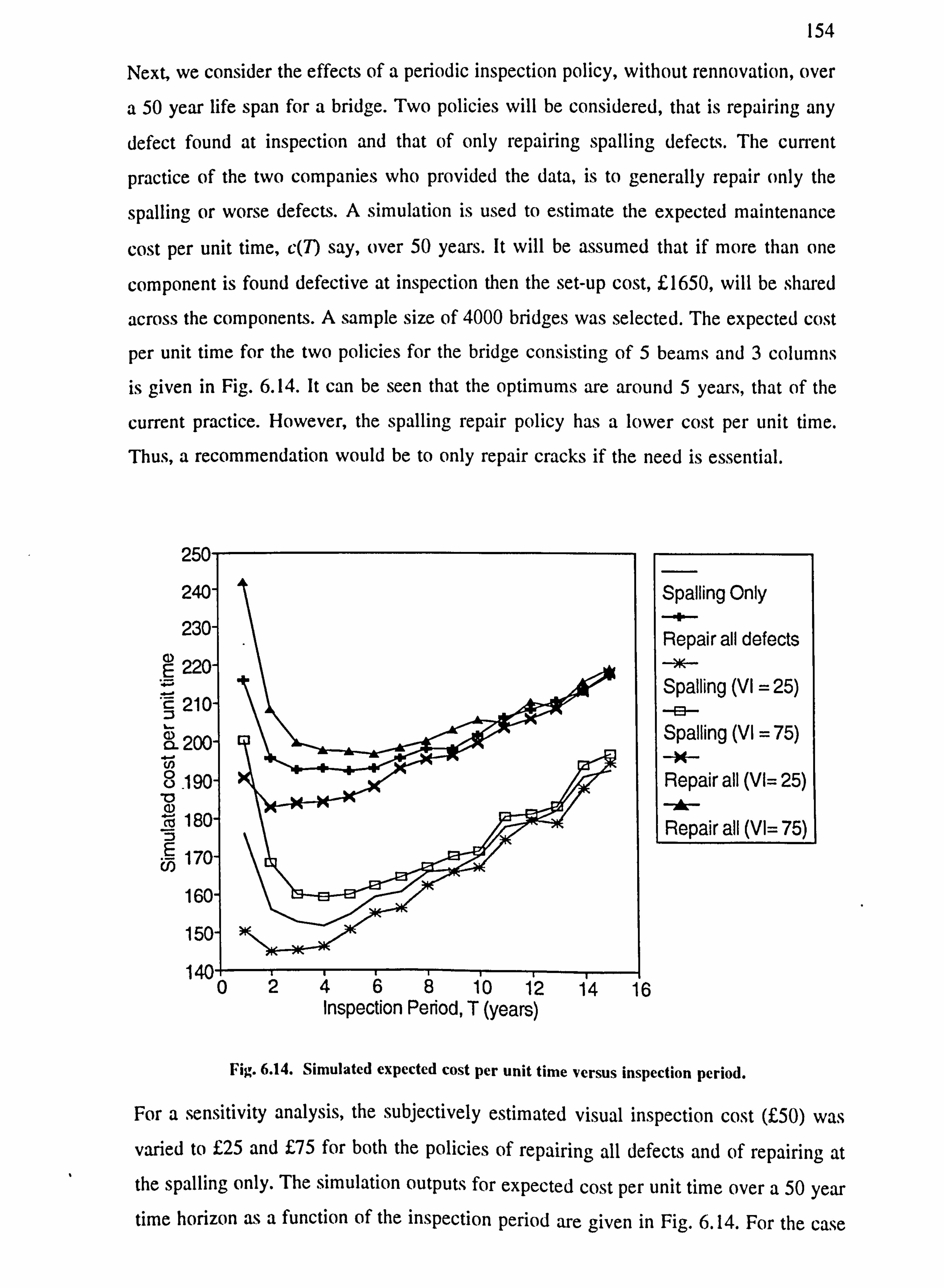
154

Next, we consider the effects of a periodic inspection policy, without rennovation, over

a 50 year life span for a bridge. Two policies will be considered, that is repairing any

defect found at inspection and that of only repairing spalling defects. The current

practice of the two companies who provided the data, is to generally repair only the

spalling or worse defects. A simulation is used to estimate the expected maintenance

cost per unit time, c(7) say, over 50 years. It will be assumed that if more than one

component is found defective at inspection then the set-up cost, £1650, will be shared

across the components. A sample size of 4000 bridges was selected. The expected cost

per unit time for the two policies for the bridge consisting of 5 beams and 3 columns

is given in Fig. 6.14. It can be seen that the optimums are around 5 years, that of the

current practice. However, the spalling repair policy has a lower cost per unit time.

Thus, a recommendation would be to only repair cracks if the need is essential.

240

E :

22

X21

a 2C Ü_is

E 17

1

1

1401 1 2468 10 12 14 Inspection Period, T (years)

16

Spalling Only

Repair all defects

Spalling (VI = 25) p

Spalling (VI = 75)

Repair all (Vl= 25) A

Repair all (Vl= 75)

Fig. 6.14. Simulated expected cost per unit time versus inspection period.

For a sensitivity analysis, the subjectively estimated visual inspection cost (£50) was

varied to £25 and £75 for both the policies of repairing all defects and of repairing at the spalling only. The simulation outputs, for expected cost per unit time over a 50 year time horizon as a function of the inspection period are given in Fig. 6.14. For the case

155

of spalling repair, the optimum inspection is reduced to 2 years for the £25 inspection

cost and still at 4 years for the £75 cost. For the case of repairing all defects, the same

reduction in the optimum can be seen for the £25 cost. However, the optimum is

increased to 6 years for the £75 inspection cost. Clearly, the requirement to a more

degradable state before repair does, in this case, lead to notably lower costs. It is also

evident that the cost of the inspection is more influential upon the inspection period

when all defects are repaired and not postponed to the spalling stage. This is consistent

with intuition.

6.6. Conclusion

The chapter has highlighted a method to model the deterioration and maintenance of

concrete structures. The concept of delay time is an important ingredient in the

modelling process, and this is extended to a four phase classification of a component;

namely defect free, cracking, spalling and failure.

Analysis of the database shows the deterioration of components over a series of

inspection and initial p. d. fs of the delay time phases have been calculated. A method to

estimate parameters with the censored data based using maximum likelihood has been

proposed, along with a technique for testing the fit obtained.

Other models for the delay time distribution have been considered. We recall that the

probability, p, that a defect will develop within 50 years, was defined due to defect

histories being, on average, recorded over this period. If interest is in a maintenance

strategy upto a 50 year time span then the time of defect developments beyond 50 years

need not be modelled. However, a defect development beyond the 50 year time span is

most likely to arise in components subjected to mild and dry environments, see Currie

and Robery (1994). Hence, the parameter I) introduced in Section 6.4 seems a reasonable

parameter to employ for modelling the initial point distribution, g(u), in the assessment

of the 50 year condition, equation (6.3). The need to introduce a probability, q, that the

cracking phase takes zero time was due to a substantial number of components being

detected first in the spalled state. It is known that the cracking phase can be short in

some cases when a component is subjected to intermittent wet conditions, see Currie and

156

Robery (1994). Hence, it is of interest to estimate this parameter.

Parameter estimation programs were successfully written and tested using simulation. The parameter estimates for beams and columns were tested using the Kaplan-Meier

estimate of the reliability function, resulting in close fits for u and u+h over 50 years

and for u+h+v over 35 years for beams and 50 years for columns, with the maximum

likelihood fit lying within 95% confidence bands of the Kaplan-Meier estimate.

Problems that arose when estimating repair costs for concrete components have already been outlined in the text. The main factors in achieving success in the current type of data collection are:

1. The questions need to be fully understood by the organization involved

in estimating.

2. Regular meetings with the repair organization and operational researchers

are important to clarify the nature and use of the information sought. 3. A large data sample is required, especially to estimate bi-variate cost

functions.

4. Timely return of costing information so that, if necessary, revised

questionnaires can be prepared within the project time.

The recent paper by Wang (1995) would have assisted us considerably here, and the

concepts will be utilised in developments when distributions of costs are required. Close

collaboration and continuous contact with civil engineers is also necessary to fully

understand the process being modelled, so that accurate predictions of concrete deterioration and cost consequences of inspection and repair practices can be formulated.

Single component and multi-component cost models were formulated incorporating the

estimated model for deterioration and the estimated cost functions. The single

component model recommends to inspect beams at around 5 years and columns at 6

years. The cost model for a bridge suggests to overhaul at around 20-30 years. The

recommended periodic inspection policy for a bridge is to inspect every 5 years, repairing only spalling defects, which interestingly is approximately the current practice

157

of the companies involved. Further research would lie in investigating the effect of

inspections prior to an overhaul or in some form of age based policy. Other extensions

relate to the stochastic distribution nature of costs and the non-perfect nature of

inspections. The sensitivity analysis, on varying the visual inspection cost, has shown

that the cost of inspection has greater influence upon the optimum inspection period for

the case of repairing all defects, compared to the practice of repairing only at the

spalling stage.

The main conclusion of the research program is that if the appropriate input data is

collected in a coherent and methodical fashion, it is possible to utilise it to model

deterioration rate, and further, the potential exists to model cost consequences of

inspection policies and thereby optimize inspection practices.

158

Chapter 7

Conclusion

7.1 Literature Review

Chapter 1 has presented an overview of past and current developments in maintenance

modelling. It is evident that delay time models and other new models are now

increasingly being applied and tested through case studies. However, there is evidence

of a deficiency of models for maintenance that takes into account the physical process,

be it chemical, electrical or mechanical, that leads to a component failure. Geraerds

(1972) regards the selection of statistical models for component and system failure

behaviour as a subsection of a complex maintenance model of an organisation, that also

takes into account such factors as maintenance planning and control, designs of systems,

inventory problems and the feedback of results. Dekker et al (1995) consider also the

planning of the maintenance activities for a group of components with different

estimated optimal policies. It is shown that combining the maintenance activities, by

delaying or bringing forward planned maintenance for some components with increased

cost penalty, can reduce overall maintenance costs. This is due to the setup cost being

shared. Hence, the necessary fusion between mathematical models and organizational

planning and constraints are evolving in the maintenance field.

Over the past ten years, since the first paper, Christer and Waller (1984a), delay time

modelling has undergone considerable development and is increasingly being accepted

as an important concept for the real world modelling of maintenance of components and

systems. There have been models which have touched on the concept, for example, Cox

(1957, p. 121) introduced a wear model such that a component can be defect free or enter

a defective state prior to failure. This is equivalent to having a finite probability of zero delay time. An inspection model is presented to take into account this effect. Cozzoloni

(1968) formulates a model whereby a system is assumed to have an unknown number

159

of defects after a planned maintenance activity with each defect having a delay to cause

failure. It is shown that the process of breakdowns will be a non-homogeneous Poisson

process, as with the delay time system model. Butler (1979) classifies a component as

functioning, functioning but defective, and failed. An inspection is also assumed to

possibly increase the chance of failure due to the chance of observing a component in

the defective state. However, a Markov model is formulated, thereby restricting the

distribution of u and h to exponential. Lewis (1972) suggests an accumulation model

whereby defective components which are detectable and do not cause failures, i. e having

infinite delay time, are repaired at a failure. The expected repair time is then correlated

with operating time.

Statistical methods, testing and policy formulations are evidently being developed and

formalised for the delay time model with the growing experience through applications.

It is important that statistical tests are carried out in confirming all postulated

assumptions, e. g the renewal assumption of a perfect inspection. A method to identify

the optimal and feasible policy type (e. g periodic or age-based inspections) for a

component or system also needs to be addressed.

7.2 Delay Time Models for Repairable Systems

It has been seen that the concept of delay time can be used in modelling maintenance

of a complex system. The NHPP model for the arrival process of failures of a repairable

system, endorsed by Ascher and Feingold (1984), incorporates the concept of delay time by allowing the ROCOF be a convolution of the defect rate and delay time p. d. f under the assumption of independence. In this way, the expected number of defects detected

at inspections can also be modelled. However, the assumption of an NHPP for a system

will need to be tested for a specific case.

The case of imperfect inspection with NHPP defect arrivals has not been considered here

and is an area for further research which is underway elsewhere. The inspection point for this case is not a system renewal implying that the defect arrival rate g(u) cannot be

considered identical in each inspection interval. This increases the modelling complexity.

160

Clearly, the downtime and cost of other inspection policies can also be investigated. For

example, a policy could be to inspect after the n'th failure occurrence or when a

particular length of operating time t has elapsed. The decision variables would be n and

t. The use-based inspection policy is when n= co. The case, n=1, implies an age based

replacement policy, for the case of perfect inspections.

Under restricted circumstances, it has been shown that the system can be modelled by

a Markov process in continuous time, see also Duyn Schouten and Wartenhorst (1994).

This model could also be expanded to the more realistic case when there are a finite

number of defect prone components within a system.

A criticism of these models is that ageing of the system after each inspection has not been modelled. Ageing can be modelled by assuming non-identical defect rates, g(u),

over each inspection interval. It is also possible to allow the delay time of a defect to

be dependent on u and the inspection interval in which the defect occurred, see Christer

and Wang (1992). The process of breakdowns then would not necessarily be an NHPP.

The type of model selected is directly dependent on assumptions on how the system is

used, type and quality of maintenance and the deterioration processes over time. The

purpose of this chapter has been to introduce the basic nature of the delay time concept

and the variety of models that may be constructed.

7.3 Updating and Estimating Parameters for Delay Time Models.

Several formal techniques of updating delay time models have been presented. These

have been based on the existence of subjective data to decide a prior or type of delay

time distribution. The prior is then parameterized under a linear transform and the

uniqueness and existence of a solution to modelling the "status quo" is discussed. It has

been found that a unique solution exists under a simple scale transform and a set of

solutions under the more general linear case. The effects of changing the model via the

parameter, ß (the probability a defect is detected at inspection), that is for ß=I to (3 #1 and vice-versa, or simply varying ß, as another updating option has also been

investigated which highlights the variety of updating options.

161

The effects of the change in the downtime model and consequently the optimum

inspection period has been demonstrated for various updating techniques. Further

research could lie in predicting the behaviour of the optimum for updating options,

modelling parameters and delay time p. d. f types.

Another method of parameter estimation has been proposed based on observed times of

breakdown and the defects detected at inspections. For this method, the prior distribution

type can be assumed and the parameters are then determined using the method of

moment or maximum likelihood technique. It has been seen that the observed failure

times can be also be used in a test for fitting a model and in deciding upon a delay time

prior when no delay time data is available.

Delay times may not only be biased subjectively, but also from a censored data set. Delay times, for example, may only be estimated from the failures which occur over a

data collection survey. Hence, an observational bias enters the problem.

7.4 Bias in the Initiation and Delay Time Parameter Estimates

It has been seen that a statistical bias can exist in the data leading to parameter estimates

of delay time and initiation time for censored data. Breakdown based observations give

rise to an underestimate of delay time and initiation time whilst observations based upon

defect repairs at inspection give rise to overestimates. The bias has been shown to be

dependent on inspection frequency and the perfectness of inspections.

Methods based on maximum likelihood have been proposed to cope with the bias and lead to the estimation of the actual initiation time and delay time distribution.

In the case of censored data, it may be possible that parameters for the delay time distribution can be estimated to an acceptable degree of accuracy by updating procedures instead of performing the bias correction. Some form of iteration method could be

proposed.

162

7.5 Simulation Study of the Delay Time Process

It has been seen that the simulation models and various parameter estimation procedures

produce results in agreement with theoretical models. This, validates the programming

of and the derivation of the delay time models and theory of the previous section. The

bias correction and iteration methods estimate the parameters of the delay time

distribution to within 10% of the theoretical values for a moderately sized sample, on

the tests carried out so far. The method of estimation using only observed data also

produces results in accordance with theory. We conclude that these are formal

techniques. However, convergence properties of the iteration method needs to be further

researched. The answer to the convergence will lie in the form of the log-likelihood

functions. It is believed, for the work required here, that if convergence occurs through

the iteration method, then the estimates will tend to the maximum likelihood estimates

when correcting for bias, as the sample size increases.

Investigation into the error of the optimum inspection period when carrying out these

method also needs research. A clue could lie in the behaviour of the function b(T; a, 'y)

for values of T, under the non-unique set ((x, y) which satisfy the observation point b',

where a and w are the scale and shift parameters respectively. The cost and downtime

curves under such restrictions, may have optimum inspection periods which lie within

a certain calculable interval. However, the measure of error, if the iteration method gives

accurate results in most cases this may not now be necessary to consider.

The criteria for deciding whether to perform iteration or bias correction produces

satisfactory results. The suggested decision procedures for deciding whether or not to

correct for bias may only work when the biased distribution can be approximated by a Weibull distribution. This occurs in the test of section 5.4.4, as the failures delay times

are almost exponential. A decision to not correct for bias may be made on the status-quo

point being satisfied. However, the resulting model for other inspection periods than the

current practice may be inaccurate. A further statistical test, such as, for example,

comparing the empirical and theoretical distribution of times of breakdowns, would need

to be applied.

163

Overall, simulation programs have been successfully written and tested, and methods

have been developed for estimating delay distributions given accurately estimated data

in practice. Further work could also lie in the effects of subjective errors when

estimating delay time, the possibility of imperfect inspections and convergence

properties of the iteration process.

7.6 Application of Delay Time Analysis to Concrete Structures

The chapter has highlighted a method to model the deterioration and maintenance of

concrete structures. The concept of delay time is an important ingredient in the

modelling process, and this is extended to a four phase classification of a component;

namely defect free, cracking, spalling and failure.

Analysis of the database shows the deterioration of components over a series of

inspection and initial p. d. fs of the delay time phases have been calculated. A method to

estimate parameters with the censored data based using maximum likelihood has been

proposed, along with a technique for testing the fit obtained.

Other models for the delay time distribution have been considered. We recall that the

probability, p, that a defect will develop within 50 years, was defined due to defect

histories being, on average, recorded over this period. If interest is in a maintenance

strategy upto a 50 year time span then the time of defect developments beyond 50 years

need not be modelled. However, a defect development beyond the 50 year time span is

most likely to arise in components subjected to mild and dry environments, see Currie

and Robery (1994). Hence, the parameter p introduced in Section 4 seems a reasonable

parameter to employ for modelling the initial point distribution, g(u), in the assessment

of the 50 year condition, equation (6.3). The need to introduce a probability, q, that the

cracking phase takes zero time was due to a substantial number of components being

detected first in the spalled state. It is knwown that the cracking phase can be short in

some cases when a component is subjected to intermittent wet conditions, see Currie and

Robery (1994). Hence, it is of interest to estimate this parameter.

Parameter estimation programs were successfully written and tested using simulation

164

The parameter estimates for beams and columns were tested using the Kaplan-Meier

estimate of the reliability function, resulting in close fits for u and u+h over 50 years

and for u+h+v over 35 years for beams and 50 years for columns, with the maximum

likelihood fit lying within 95% confidence bands of the Kaplan-Meier estimate.

Problems that arose when estimating repair costs for concrete components have already

been outlined in the text. The main factors in achieving success in the current type of

data collection are:

1. The questions need to be fully understood by the organization involved

in estimating.

2. Regular meetings with the repair organization and operational researchers

are important to clarify the nature and use of the information sought.

3. A large data sample is required, especially to estimate bi-variate cost

functions.

4. Timely return of costing information so that, if necessary, revised

questionnaires can be prepared within the project time.

The recent paper by Wang (1995) would have assisted us considerably here, and the

concepts will be utilised in developments when distributions of costs are required. Close

collaboration and continuous contact with civil engineers is also necessary to fully

understand the process being modelled, so that accurate' predictions of concrete

deterioration and cost consequences of inspection and repair practices can be formulated.

Single component and multi-component cost models were formulated incorporating the

estimated model for deterioration and the estimated cost functions. The single

component model recommends to inspect beams at around 5 years and columns at 6

years. The cost model for a bridge suggests to overhaul at around 20-30 years. The

recommended periodic inspection policy for a bridge is to inspect every 5 years,

repairing only spalling defects, which interestingly is approximately the current practice

of the companies involved. Further research would lie in investigating the effect of

inspections prior to an overhaul or in some form of age based policy. Other extensions

relate to the stochastic distribution nature of costs and the non-perfect nature of

165

inspections. The sensitivity analysis, on varying the visual inspection cost, has shown

that the cost of inspection has greater influence upon the optimum inspection period for

the case of repairing all defects, compared to the practice of repairing only at the

spalling stage.

The main conclusion of the research program is that if the appropriate input data is

collected in a coherent and methodical fashion, it is possible to utilise it to model

deterioration rate, and further, the potential exists to model cost consequences of

inspection policies and thereby optimize inspection practices.

166

Appendix

Stochastic Case Model for Downtime

An outline is given here on obtaining a more general model for downtime, that is

relaxing assumption (b), db « T, from Section 2.5. What is required is the expected

cumulative downtime over a real time interval, say (0,7). It is a more complicated

option because at time T the system could either be operating or down for repair. Hence,

the model would be dependent on knowledge of the p. d. f of the breakdown repair time.

Chilcott and Christer (1991) develop an iterative equation method for a similar problem.

Dagpunar and Jack (1993) derive a minimal repair model for a system with the

assumption of constant breakdown repair times. Hence, a need could arise for this

refinement.

Let DT, denote the cumulative breakdown repair time over interval (0, T). If no failures

have arisen in interval (0, T) then this implies P{DT = 0) = e-'(), due to NHPP

breakdown arrivals. Consider the joint event; { the system is up at time T, DT is in the

small interval (x, x+ dx), n failures have arisen over (0, T) and have been completely

repaired l. This is equivalent to having only n breakdowns in operating time t=T-x

and the cumulative breakdown time of n complete repairs in interval (x, x+ dx).

The joint probability of this event is, P{B,.. x = n}zn(x)dx, where zn(x) is the n-fold

convolution of the p. d. f for each breakdown repair time and P{ Bt = n) is given by

function (2.4).

Secondly, consider the above joint event above when the system is now down at time

T, and the n+l'th breakdown is being repaired at time T. DT will now have a

contribution from the last and incomplete repair. This event is equivalent to n failures

in operating time t=T-x, an additional failure in operating time interval

(T - x, T-x+ dx) and x spanning the interval of the n'th and n+l'th cumulative breakdown repair time. The probability of the joint event under

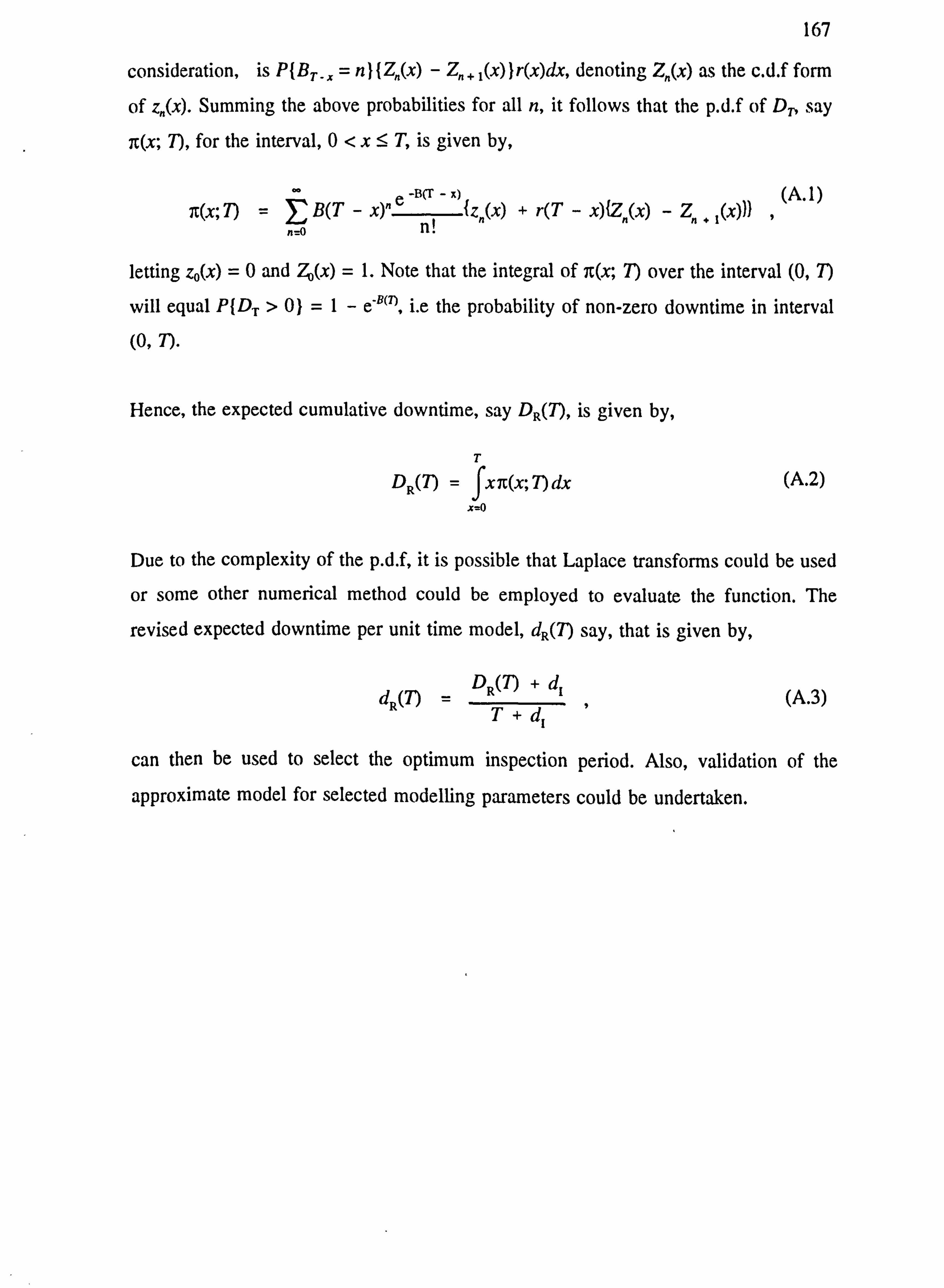
167

consideration, is P{BT_,, = n}{Z,, (x) - Zn+l(x)}r(x)dx, denoting Z,, (x) as the c. d. f form

of zn(x). Summing the above probabilities for all n, it follows that the p. d. f of DT, say

n(x; T), for the interval, 0<x: 5- T, is given by,

n(x; 7) =E B(T -x) nx) e {z(x) + r(T - x){Zn(x) -Z+ (x))} , (A. 1)

n-0 n!

letting zo(x) =0 and Z3(x) = 1. Note that the integral of it(x; 7) over the interval (0,7)

will equal P{DT > 0} =1-e -"('I, i. e the probability of non-zero downtime in interval

(0, T).

Hence, the expected cumulative downtime, say DR(T), is given by,

T

DR(T) = fxir(x; T)dx (A. 2)

x=o

Due to the complexity of the p. d. f, it is possible that Laplace transforms could be used

or some other numerical method could be employed to evaluate the function. The

revised expected downtime per unit time model, dR(T) say, that is given by,

dR(7) = DRM + dj

(A. 3)

can then be used to select the optimum inspection period. Also, validation of the

approximate model for selected modelling parameters could be undertaken.

168

References

Ascher, H. (1992), Basic probabilistic and statistical concepts for maintenance of parts

and systems, IMA Journal of Mathematics Applied in Business and Industry, 3,153-167.

Ascher, H. and Feingold, H. (1984), Repairable Systems Reliability, Marcel Dekker,

New York.

Baker, R. D., (1991), Testing the efficacy of preventive maintenance, Journal of the

Operational Society, 42,494-503.

Baker, R. D. and Christer, A. H. (1994), Operational Research modelling of engineering

aspects of maintenance, European Journal of Operational Research, 73,407-422.

Baker, R. D. and Wang, W. (1992), Estimating the delay-time distribution of faults in

repairable machinery from failure data, IMA. Journal of Mathematics Applied in Business

and Industry, 3,259-281.

Baker, R. D. and Wang, W (1993), Developing and testing the delay time model,

Journal of the Operational Research Society, 44,361-374.

Barlow, R. E. (1984), Mathematical theory of reliability: an historic perspective, IEEE

Transactions on Reliability, R-33,1,16-19.

Barlow, R. E. and Hunter, L. C. (1960a), Optimal preventive maintenance policies,

Operations Research, 8,90-100.

Barlow, R. E. and Hunter, L. C. (1960b), Reliability analysis of a one-unit system,

Operations Research, 9,200-208.

Barlow, R. E. and Proschan, F. (1965), Mathematical Theory of Reliability, Wiley, New

York.

169

Beichelt, F. (1981), Minimax inspection strategies for single unit systems, Naval

Research Logistics, 28,375-381.

Butler, D. A. (1979), A hazardous inspection model, Management Science, 25,79-89.

Cerone, P. (1991), On a simplified delay time model of reliability of equipment subject

to inspection monitoring, Journal of the Operational Research Society, 42,505-511.

Chatfield, C. (1970), Statistics for Technology, Chapman and Hall, New York.

Chilcott, J. B. and Christer, A. H. (1991), Modelling of condition based maintenance at the coal face, International Journal of Production Economics, 22,1-11.

Cho, D. I. and Parlar, M. (1991), A survey of maintenance models for multi-unit

systems, European Journal of Operational Research, 51,1-23.

Christer, A. H. (1973), Innovatory decision making, The Role and Effectiveness of Theories of Decision in Practice, Hodder & Stoughton, London, 368-377.

Christer, A. H. (1978), Refined asymptotic costs for renewal reward processes, Journal

of the Operational Research Society, 29,577-584.

Christer, A. H. (1982), Modelling inspection policies for building maintenance, Journal

of the Operational Research Society, 33,723-732.

Christer, A. H. (1984), Operational research applied to industrial maintenance and replacement, In: Developments in OR (R. W. Eglese & G. W. Rand Eds. ), Perganuon

Press.

Christer, A. H. (1987a), Delay-time of reliability of equipment subject to inspection

monitoring, Journal of the Operational Research Society, 38,329-334.

170

Christer, A. H. (1987b), Comments on finite-period application of age-based replacement

models, IMA Journal of Mathematics in Management, 1,111-124.

Christer, A. H. (1988), Condition-based inspection models of major civil-engineering

structures, Journal of the Operational Research Society, 39,71-82.

Christer, A. H. (1992), Proto-type model of irregular condition monitoring of production

plant, IMA Journal of Mathematics Applied in Business and Industry, 3,219-232.

Christer, A. H., Wang, W., Baker, R. D. and Sharp, J. (1995), Modelling maintenance

practice of production plant using the delay time concept, IMA Journal of Mathematics

Applied in Business and Industry, 6,67-83.

Christer, A. H. and Desa, I. M. (1992), Maintenance and availablity modelling of bus

transport in Malaysia: Issues and Problems, Proceedings of the International Conference

on OR for Developing Countries, Ahmedebad, India.

Christer, A. H. and Jack, N. (1991), An integral-equation approach for replacement

modelling over finite time horizons, IMA Journal of Mathematics Applied in Business

and Industry, 3,31-44.

Christer, A. H. and Keddie, E. (1985), Experience with a stocahstic replacement model, Journal of the Operational Research Society, 36,25-34.

Christer, A. H. and Redmond, D. F. (1990), A recent mathematical development in

maintenance theory, IMA Journal of Mathematics Applied in Business and Industry, 2,

p. 97-108.

Christer, A. H. and Redmond, D. F. (1992), Revising models of maintenance and inspection, International Journal of Production Economics, 24,227-234.

Christer, A. H. and Scarf, P. A. (1991), A robust replacement model, Journal of the Operational Research Society, 45,261-275.

171

Christer, A. H. and Waller, W. M. (1984a), Delay-time models of industrial inspection

and maintenance problems, Journal of the Operational Research Society, 35,401-406.

Christer, A. H. and Waller, W. M. (1984b), Reducing production downtime using delay-

time analysis, Journal of the Operational Research Society, 35,499-512.

Christer, A. H. and Waller, W. M. (1984c), An OR approach to planned maintenance: Modelling P. M. for a vehicle fleet, Journal of the Operational Research Society, 35,

p. 967-512.

Christer, A. H. and Wang, W. (1992), A model of condition monitoring of a production

plant, International Journal of Production Research, 30,2199-2211.

Christer, A. H. and Wang, W. (1995), A simple condition monitoring model for a direct

monitoring process, European Journal of Operational Research, 82,258-269.

Cox, D. R. (1957), Renewal Theory, Chapman and Hall, London.

Cox, D. R. and Hinkley, D. V. (1974), Theoretical Statistics, Chapman and Hall.

Cox, D. R. and Lewis, P. A. W. (1966), The Statistical Analysis of Survival Data,

Chapman and Hall, London.

Cox, D. R. and Miller, H. D. (1965), The Theory of Stochastic Processes, Methuen.

Cox, D. R. and Oakes, D. (1983), Analysis of Survival Data, Chapman and Hall.

Cozzolino Jr., J. M. (1968), Probabilistic models of decreasing failure rate processes, Naval Research Logistics Quarterly, 15,361-374.

Currie, R. J. and Robery, P. C. (1994), Repair and Maintenance of Concrete Structure,

Building Research Establishment, No. BR 2-0851256236.

172

Dagpunar, J. S. (1994), Some necessary and sufficient conditions for age replacement

with non-zero downtimes, Journal of the Operational Research Society, 45,2,225-229.

Dagpunar, J. S. and Jack, N. (1993), Optimizing system availability under minimal

repair with non-negligible repair and replacement times, Journal of the Operational

Research Society, 11,1097-1104.

Dekker, R., Smit, A. and Losekoot, J. (1995), Combining maintenance activities in an

operational planning phase: a set partitioning approach, IMA Journal of Mathematics

Applied in Business and Industry, 3,315-331.

Van der Duyn Schouten, F. A and Wartenhorst, P. (1994). Transient analysis fo a two-

unit standby system with Markovian degrading units, Management Science, 40,418-428.

Edwards, A. W. F. (1972), Likelihood, Cambridge University Press.

Feller, W. (1970a), An Introduction to Probability Theory and its Applications, Vol. I,

Wiley, New York.

Feller, W. (1970b), An Introduction to Probability Theory and its Applications, Vol. II,

Wiley, New York.

Geraerds, W. M. J. (1972), Towards a theory of maintenance, In: On the Organization

of Logistic Support Systems, The English University Press, London, 297-329.

Gits, B. (1986), On the Maintenance Concept for a Technical System, 1, Maintenance

Management International, 6,131-146.

Grimmett, G. R. and Strirzaker, D. R. (1982), Probability and Random Processes, Oxford

University Press.

Jack, N. (1991), Repair replacement modelling over finite time horizons, Journal of the

Operational Research Society, 42,759-766.

173

Jack, N. (1992), Costing a finite minimal repair replacement policy, Journal of the

Operational Research Society, 43,3,271-275.

Jack, N. and Dagpunar, J. S. (1992), Costing minimal-repair replacement policies over

finite time horizons, IMA Journal of Mathematics Applied in Business and Industry,

3,207-217.

Jansen J. and Van der Duyn Schouten, F. A. (1995), Maintenance optimization on

parallel production units, IMA Journal of Mathematics Applied in Business and Industry,

6,113-134.

Jardine, A. K. S. (1973), Maintenance, Replacement and Reliability, Pitman Publishing,

London.

Jardine, A. K. S. and Hassounah, M. I. (1990), An optimal vehicle-fleet inspection

schedule, Journal of the Operational Research Society, 41,791-799.

Kalbeisch, J. D and Prentice, R. L. (1980), The Statistical Analysis of Failure Time

Data, Wiley, New York.

Kaio, N. and Osaki, S. (1989), Comparison of inspection policies, Journal of the

Operational Research Society, 40,5,499-503.

Khintchine, A. Y. (1932), Mathematisches über die Ewartung von einen öffenlicher

Schalter, Matent. Sbornik.

Khintchine, A. Y. (1960), Mathematical Methods in the Theory of Queuing, Griffin,

London.

Kijima, M., Morimura, H. and Suziki, Y. (1988), Periodical replacement problem

without assuming minimal repair, European Journal of Operational Research, 37,194-

203.

174

Kobbacy, K. A. H., Percy, D. F. and Fawzi, B. B. (1995), Sensitivity analysis for

preventive maintenance models, IMA Journal of Mathematics Applied in Business and

Industry, 6,53-66.

Lewis, P. (1972), Stochastic Point Processes: Statistical Analysis Theory and

Applications, Wiley, New York.

Maisel, H. and Gnugnoli, G. (1972), Simulation of Discrete Stochastic Systems, Science

Research Associates.

Makis, V. and Jardine, A. K. S. (1992), Optimal replacement policy for a general model

with imperfect repair, Journal of the Operational Research Society, 43,2,111-120.

McCall, J. J. (1965), Maintenance policies for stochastically failing equipment: a survey,

IEEE Transactions on Reliability, 28,133-136.

Medhi, J. (1983), Stochastic Processes, Wiley Eastern.

Morimura, H. (1970), On some preventive maintenance policies for IFR, Journal of the

Operational Research Society Japan, 12,94-125.

Nelson, W. (1984), Applied Life Data Analysis, Wiley, New York.

Parzen, E. (1962), Probability and Random Processes, McGraw-Hill.

Pelligrin, C. (1991), A graphical procedure for an on-condition maintenance policy:

imperfect-inspection model and interpretation, IMA Journal of Mathematics Applied in

Business and Industry, 3,177-191.

Pierskella, W. P. and Voelker J. A. (1976), A survey of maintenance models: the

control and surveilance of deteriorating systems, Naval Research Logistics Quarterly,

23,353-388.

175

Rigden S. R., Burley, E. and Christer, A. H. (1988), Inspection Practices for Concrete

Structures in the U. K, in: Chapter 6 in the Life of Structures, Butterworths.

RILEM (1988), Corrosion of Steel in Concrete, edited by P. Schiessl, Chapman and Hull.

Ross, S. (1983), Stochastic Processes, Wiley.

Scarf, P. A. and Bouamra, O. (1995), On the application of a capital replacement model for a mixed fleet, IMA Journal of Mathematics Applied in Business and Industry, 6,

53-66.

Smith, D. J. (1985), Reliability and Maintainability in Perspective, MacMillan.

Thomas, L. C. (1986), A survey of maintenance and replacement models for

maintainability of multi-item systems, Reliability Engineering, 16,297-309.

Thomas, L. C., Gaver, D. P. and Jacobs, P. A. (1991), Inspection models and their

application, IMA Journal of Mathematics Applied in Business and Industry, 3,283-303.

Waddington, C. H. (1973), O. R. in World War II: OR against the U-Boat, Elek Science,

London.

Valdez-Flores, C. and Feldman, R. M. (1989), A survey of preventive maintenance

models for stochastically deteriorating single-unit systems, Naval Research Logistics

Quarterly, 36,419-446.

Vanneste, S. G. and Wassenhove, L. N. (1995), An integrated and structured approach

to improved maintenance, European Journal of Operational Research, 2,241-257.

Wang, W. (1995), Subjective estimation of the delay time distribution in maintenance

modelling, to appear in European Journal of Operational Research.

delay time analysis in maintenance

Documents