Delays in Control Systems Anyone who has ever tried to stay comfortable while showering in a crowded building with old plumbing understands how delays in a system can make the control problem much more difficult. It’s not that the delays can’t be incorporated into the system model; that’s easy in sampled-data systems and certainly possible in continuous systems. If you are able design a controller that stabilizes a system containing significant delays, it will likely result in a disappointingly slow response. In general, you will find that the effects of delays in closed-loop feedback systems resemble the effects of lowering the sampling frequency. Physically, this makes sense: in both cases, the controller is forced to make use of “old” information (information about the output at some time in the past, rather than in the present) in determining the output it supplies to the plant. Modeling Delays 1. Continuous systems The Laplace transform for a pure delay is just

)()( sFetf sττ −⇔− . where τ is the delay time in seconds. Thus, it’s easy to derive transfer functions for systems containing delays. For example, a system with a cascade controller and unity feedback, but using an output sensor that is τ seconds late in reporting the output ( a sensor delay) would have a transfer function calculated from a diagram like this:

The transfer function would have the form,

]exp[)()(1)()()(

τssGsCsGsCsH

−+=

If the delay occurred in transmitting the output of the controller, C(s), to the plant (an actuator delay), the block diagram and the transfer function would look like this:

with H(s) given by

]exp[)()(1)()(]exp[)(

ττ

ssGsCsGsCssH

−+−= .

Note that the second transfer function is just a delayed version of the first. Specifically, in the frequency domain, the gain vs. frequency curves will be the same for both. The biggest obstacle to handling delay in design is not in the modeling, which you can see is quite simple: the problem lies in the fact that the delay cannot be expressed as a rational polynomial. There are some approximations that have rational polynomial forms:

......6

)(2)(1}exp{

32 ττττ ssss −+−≅− , or

...6

)(2)(1

1}exp{ 32 ττττ

ssss

+++≅− , or

2121

}exp{τ

ττ

s

ss

+

−≅− , or

n

ns

s

⎥⎦⎤

⎢⎣⎡ +

≅−τ

τ1

1}exp{ .

The last of these can be made as accurate as needed by choosing n large enough. A little experimentation with your design software will illustrate the strengths and weaknesses of these approximations. To be “valid” for a particular design, the approximation you use should accurately track (in both magnitude and phase) the Bode plot of exp{jωτ}over the range of frequencies corresponding to the bandwidth of the designed system.

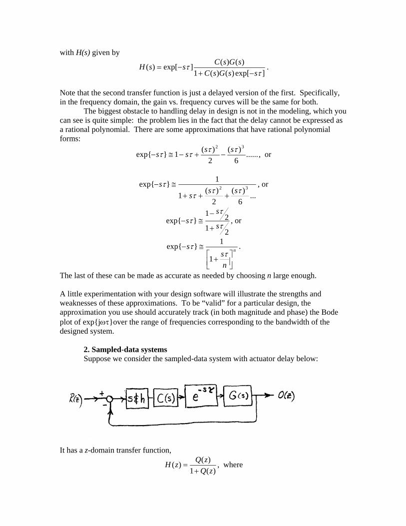
2. Sampled-data systems Suppose we consider the sampled-data system with actuator delay below:

It has a z-domain transfer function,

)(1)()(zQ

zQzH+

= , where

⎭⎬⎫

⎩⎨⎧ℑ

−≈

⎭⎬⎫

⎩⎨⎧ −

ℑ−

= −

ssGsC

zzz

sssGsC

zzzQ N )()(1]exp[)()(1)( τ , and

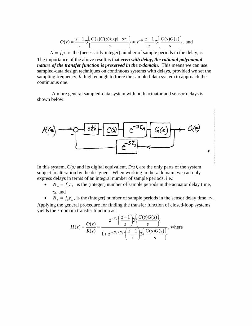
τsfN = is the (necessarily integer) number of sample periods in the delay, τ. The importance of the above result is that even with delay, the rational polynomial nature of the transfer function is preserved in the z-domain. This means we can use sampled-data design techniques on continuous systems with delays, provided we set the sampling frequency, fs, high enough to force the sampled-data system to approach the continuous one. A more general sampled-data system with both actuator and sensor delays is shown below.

In this system, C(s) and its digital equivalent, D(z), are the only parts of the system subject to alteration by the designer. When working in the z-domain, we can only express delays in terms of an integral number of sample periods, i.e.:

• AsA fN τ= is the (integer) number of sample periods in the actuator delay time, τA, and

• SsS fN τ= , is the (integer) number of sample periods in the sensor delay time, τS. Applying the general procedure for finding the transfer function of closed-loop systems yields the z-domain transfer function as

⎭⎬⎫

⎩⎨⎧ℑ⎟

⎠⎞

⎜⎝⎛ −

+

⎭⎬⎫

⎩⎨⎧ℑ⎟

⎠⎞

⎜⎝⎛ −

==+−

−

ssGsC

zzz

ssGsC

zzz

zRzOzH

SA

A

NN

N

)()(11

)()(1

)()()(

)(, where

System design with delays 1. Continuous systems You can incorporate any rational polynomial approximation for a delay into the transfer functions for the plant or the feedback loop, and then procede with the design process as you would have done in the absence of any delays. When you are finished with the design, you should check the approximation for G(s) you used in the frequency domain to see that its Bode plot closely follows one for G(s) exp{-jωτ} over all frequencies within the bandwidth of the design. Alternatively, and perhaps more safely, you can design your continuous system in the z-domain, where delays can be modeled exactly, provided you use a high sampling frequency. In the limit of very large sampling frequency, the sampled-data system will perform like the continuous one. If you use the z-domain design approach, you can start your design process neglecting delays and introduce them gradually in order to see how delay degrades the performance of the closed-loop system. 2. Sampled-data design In addition to being useful in the design of continuous systems containing delays, as discussed above, sampled-data design techniques are of course necessary for systems where the controller will be implemented digitally. Because the z-domain parameters of controllers vary as sampling frequency is changed, it will be more convenient to design the controller in the s-domain and then transform it to the equivalent z-domain transfer function, D(z).