Delft University of Technology

Effect of regenerative braking on energy-efficient train control

Scheepmaker, Gerben; Goverde, Rob

Publication date2015Document VersionPublisher's PDF, also known as Version of recordPublished inll

Citation (APA)Scheepmaker, G., & Goverde, R. (2015). Effect of regenerative braking on energy-efficient train control. In ll

Important noteTo cite this publication, please use the final published version (if applicable).Please check the document version above.

CopyrightOther than for strictly personal use, it is not permitted to download, forward or distribute the text or part of it, without the consentof the author(s) and/or copyright holder(s), unless the work is under an open content license such as Creative Commons.

Takedown policyPlease contact us and provide details if you believe this document breaches copyrights.We will remove access to the work immediately and investigate your claim.

This work is downloaded from Delft University of Technology.For technical reasons the number of authors shown on this cover page is limited to a maximum of 10.

CASPT 2015

Effect of regenerative braking on energy-efficient traincontrol

Gerben M. Scheepmaker ·Rob M.P. Goverde

Abstract An important topic to reduce the energy consumption in railwaysis the use of energy-efficient train control (EETC). Modern trains allow regen-erative braking where the released kinetic energy can be reused. This regener-ative braking has an effect on the optimal driving regimes compared to trainswhich can only use mechanical braking. This paper compares the impact ofregenerative braking on the optimal train control strategy on level track. Theenergy-efficient train control problem is modelled as an optimal control prob-lem over distance and solved using a Pseudospectral Method. Three differentbraking strategies are compared: mechanical braking only, a combination ofmechanical and regenerative braking, and regenerative braking only. The re-sult of a case study show that energy savings of at least 28% are possible byincluding regenerative braking.

Keywords Energy efficiency · optimal train control · regenerative braking

1 Introduction

Railway undertakings (RUs) are taking various measures to decrease energyconsumption. Energy-efficient train control is an effective mean to reduce op-erating energy costs and so a lot of research is devoted to this area. Most of

Gerben M. ScheepmakerNetherlands Railways, Department of LogisticsP.O. Box 2025, 3500 HA Utrecht, The NetherlandsDelft University of Technology, Department of Transport and PlanningP.O. Box 5048, 2600 GA Delft, The NetherlandsTel.: +31 (0)15 27 84914E-mail: g.m.scheepmaker@tudelft.nl

Rob M.P. GoverdeDelft University of Technology, Department of Transport and PlanningP.O. Box 5048, 2600 GA Delft, The Netherlands

this research is based on optimal control theory, and in particular Pontrya-gin’s Maximum Principle (PMP) (Pontryagin et al, 1962) has been applied toderive the necessary optimality conditions that characterize the optimal con-trol structure (Howlett, 1996; Khmelnitsky, 2000; Liu and Golovitcher, 2003;Scheepmaker and Goverde, 2015). The optimal control consists of a sequenceof the optimal driving regimes maximum acceleration (MA), cruising (CR),coasting (CO), and maximum braking (MB). Given this knowledge of the op-timal driving regimes, most train control algorithms then aim at finding theoptimal switching points between the regimes.

However, most literature did not consider the possibility for regenerativebraking, but only mechanical braking in which braking energy is transformedinto heat. In regenerative braking, the released kinetic energy, generated bythe engine of the train during braking (using electro-dynamic brakes), is sentback to the catenary system to be used by other surrounding trains. Moreand more trains nowadays have the ability to apply regenerative braking andtherefore its impact on the optimal control strategy becomes highly relevant.

Asnis et al (1985) were the first to incorporate regenerative braking in theenergy-efficient train control problem. They included regenerative braking inthe objective function as a percentage of the total braking force and derivedthe necessary conditions for the optimal control strategy. In addition to thefour basic optimal driving regimes, they found a fifth optimal driving regime ofregenerative braking (RB). However, they did not provide an algorithm to findthe optimal sequence and switching times of the driving regimes. Khmelnitsky(2000) also considered the train control problem with regenerative braking. Hefound the same optimal control structure as Asnis et al (1985) and described anumerical method to solve the problem including varying gradients and speedlimits. In an example he showed that regenerative braking was used to sta-bilize the cruising speed on downward slopes. Franke et al (2000) simplifiedthe train resistance function and derived analytical expressions for the variousdriving regimes. They solved the problem by discrete dynamic programmingand applied it to a case study. However, they did not provide details on theoptimal sequence of driving regimes, but only mentioned that a main part ofthe computed energy saving resulted from the reduced use of the mechanicalbrakes. Baranov et al (2011) considered the train control problem consider-ing both mechanical and regenerative braking in their objective function, andalso included the efficiency of regenerative braking. They derived seven driv-ing regimes: the three familiar regimes MA, CO and MB (maximum brakingwith both mechanical and regenerative braking), three cruising regimes witheither partial traction (CR), partial regenerative braking (RB) or with full re-generative braking and partial mechanical braking, and finally a regime withfull regenerative braking. An algorithm to construct the optimal control se-quence of these driving regimes was mentioned as an open question. Rodrigoet al (2013) considered a discretized optimal train control problem includingefficiency of regenerative braking and they considered both mechanical and re-generative braking for a metro system. They concluded from their metro sim-ulations that regenerative braking from higher speeds is more efficient than

coasting, so they replace coasting by regenerative braking. Qu et al (2014)also considered metro systems and assume fully regenerative braking (no me-chanical braking). They assume that the optimal driving strategy consist onlyof maximum acceleration, cruising and maximum regenerative braking. Theyprovide an algorithm to calculate the optimal cruising speed and applied it toa case study of a metro line, but without reporting any energy savings.

In summary, the literature reports different impacts of regenerative brak-ing on the energy-efficient train control depending on the assumptions andconditions. Therefore, this paper considers the energy-efficient train controlproblem with both mechanical and regenerative braking including efficiencyand considers a case study for a main line local passenger train. In this paperwe assume level track to focus on the structure of the optimal driving strategywithout the influence of gradients.

Section 2 gives the energy-efficient rain control problem without and withregenerative braking. Section 3 explains the algorithm applied to solve thetrain control problem problem, after which the model is applied on a casestudy of the Netherlands Railways (NS) in Section 4. Finally, Section 5 endsthe paper with conclusions.

2 Model description

This section describes the energy-efficient train control (EETC) problem andderives the structure of the optimal driving regimes.

Consider the problem of driving a train between two stops in a given timewith minimal energy consumption. Let X be the stop distance, T the scheduledrunning time. We use distance x as the independent variable and time t(x) andspeed v(x) as function of position as the state variables. The control variableis the mass-specific force u(x). The control variable can be partitioned into anonnegative traction force and a negative braking force which are indicatedas u+ = max(u, 0) and u− = min(u, 0), respectively. Note that implicitlyu+ · u− = 0, i.e., if u+ is nonzero than u− = 0 and vice versa, correspondingto the fact that trains do not give traction and brake at the same time.

Without regenerative braking, the energy-efficient train control problemcan be formulated as (Scheepmaker and Goverde, 2015)

J = minu

∫ X

0

u+(x)dx (1)

subject to

t′(x) = 1/v (2)

v′(x) = (u− r(v))/v (3)

t(0) = 0, t(X) = T, v(0) = 0, v(X) = 0 (4)

v(x) ∈ [0, vmax], u(x) ∈ [−umin, umax(v(x))]. (5)

The specific traction and braking force u(x) are the forces acting on the traindivided by total mass, including a rotating mass factor. The maximum mass-specific traction is a non-increasing function of speed. An example of the trac-tion control-speed diagram with both a constant and hyperbolic part can befound in figure 1. The maximum braking is assumed to be constant. The mass-specific resistance force r(v) = r0 + r1v+ r2v

2 is a positive quadratic functionof speed (Davis, 1926).

Fig. 1 Traction control-speed diagram for rolling stock type SLT-6 of NS

This problem can be solved by using optimal control theory. Pontryagin’sMaximum Principle (PMP) can be applied to derive necessary conditions forthe optimal control (Pontryagin et al, 1962). For this define the Hamiltonian

H(t, v, ϕ, λ, u) = −u+ +φ

v+λ(u− r(v))

v

=

{(λv − 1)u+ ϕ

v −λr(v)v if u ≥ 0

λvu+ ϕ

v −λr(v)v if u < 0,

(6)

where ϕ(x) and λ(x) are the co-state variables satisfying the adjoint differentialequations

ϕ′(x) = −∂H∂t

= 0 (7)

λ′(x) = −∂H∂v

=λu+ λvr′(v)− λr(v) + ϕ

v2. (8)

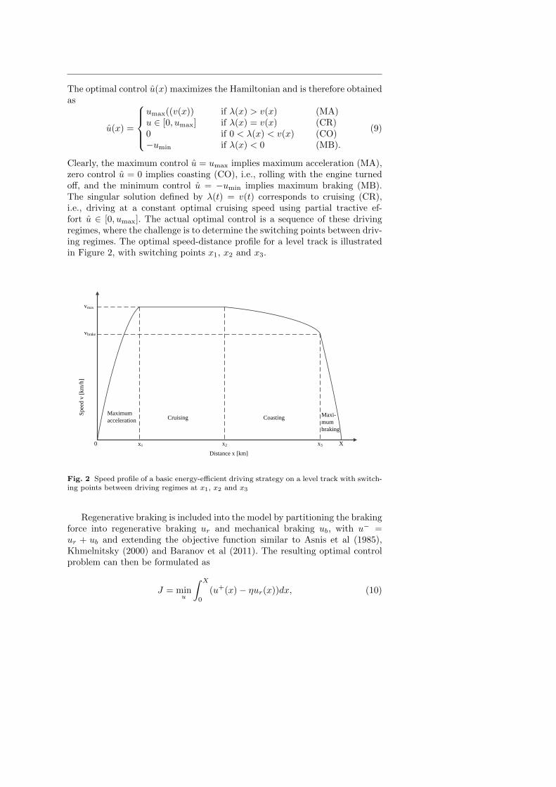
The optimal control u(x) maximizes the Hamiltonian and is therefore obtainedas

u(x) =

umax((v(x)) if λ(x) > v(x) (MA)u ∈ [0, umax] if λ(x) = v(x) (CR)0 if 0 < λ(x) < v(x) (CO)−umin if λ(x) < 0 (MB).

(9)

Clearly, the maximum control u = umax implies maximum acceleration (MA),zero control u = 0 implies coasting (CO), i.e., rolling with the engine turnedoff, and the minimum control u = −umin implies maximum braking (MB).The singular solution defined by λ(t) = v(t) corresponds to cruising (CR),i.e., driving at a constant optimal cruising speed using partial tractive ef-fort u ∈ [0, umax]. The actual optimal control is a sequence of these drivingregimes, where the challenge is to determine the switching points between driv-ing regimes. The optimal speed-distance profile for a level track is illustratedin Figure 2, with switching points x1, x2 and x3.

vmax

vbrake

x1 x2 x3 X

Distance x [km]

Spee

d v

[km

/h]

0

Maximum

accelerationCruising Coasting

Maxi-

mum

braking

Fig. 2 Speed profile of a basic energy-efficient driving strategy on a level track with switch-ing points between driving regimes at x1, x2 and x3

Regenerative braking is included into the model by partitioning the brakingforce into regenerative braking ur and mechanical braking ub, with u− =ur + ub and extending the objective function similar to Asnis et al (1985),Khmelnitsky (2000) and Baranov et al (2011). The resulting optimal controlproblem can then be formulated as

J = minu

∫ X

0

(u+(x)− ηur(x))dx, (10)

subject to

t′(x) = 1/v (11)

v′(x) = (u+ − ur − ub − r(v))/v (12)

t(0) = 0, t(X) = T, v(0) = 0, v(X) = 0 (13)

v(x) ∈ [0, vmax] (14)

u+(x) ∈ [0, umax(v(x))], ur ∈ [0, ur], ub ∈ [0, ub] (15)

where η ∈ [0, 1] is the efficiency of the regenerative braking system, ur is themaximum regenerative braking, and ub is the maximum mechanical brakingwith ur + ub = umin.

The resulting optimal control structure is now less obvious, since now thereare three control variables with two braking controls. This leads to several op-tions for braking by a combination of regenerative and mechanical braking,with the most likely according to Baranov et al (2011) being partial regenera-tive braking, maximum regenerative braking, maximum regenerative brakingwith partial mechanical braking, and maximum braking with both full mechan-ical and regenerative braking. The next section describes a direct algorithmto find the optimal control strategy without requiring a priori the structure ofthe optimal regimes.

3 Direct solution method

Numerical methods for solving optimal control problems are divided into twomajor classes: indirect methods and direct methods (Betts, 2010). In an in-direct method, first necessary optimality conditions are derived based on e.g.Pontryagin’s Maximum Principle. Then a solution is found satisfying the nec-essary optimality conditions which thus indirectly solved the original problem.This approach has been the preferred method in the train control community,where the original optimal control problem is translated into a finite optimiza-tion problem of finding the optimal sequence of optimal driving regimes andtheir switching points.

In a direct method, the state and/or control variables of the optimal controlproblem are discretized and the problem is transcribed to a nonlinear program-ming problem (NLP) (Betts, 2010). The NLP is then solved using well-knownnonlinear optimization techniques. In particular, Pseudospectral methods havebeen proven themselves in solving optimal control problems efficiently (Rao,2003). In Pseudospectral methods the control and state variables are param-eterized by polynomials with exact values at the so-called collocation points.We applied the Gauss Pseudospectral Method (GPM) that uses orthogonalcollocation at Legendre-Gauss points. For more details, see Rao (2003). In thetrain control community direct methods have been used only recently. Wanget al (2013) solved an optimal train control problem by transcribing it to botha GPM and a Mixed Integer Liner Programming Problem, and Wang et al(2015) used GPM to solve an optimal train control problem.

An efficient implementation of GPM is provided in the MATLAB tool-box GPOPS (General Pseudospectral OPtimal Control Software) (Rao et al,2010a). We used Radau Pseudospectral method in GPOPS together with theautomatic differentiator INTerval LABoratory (INTLAB) (Rao et al, 2010b;Rump, 1999).

4 Case study and results

The model called EZ3R model is tested in a case study. This case study andthe results are discussed in this section.

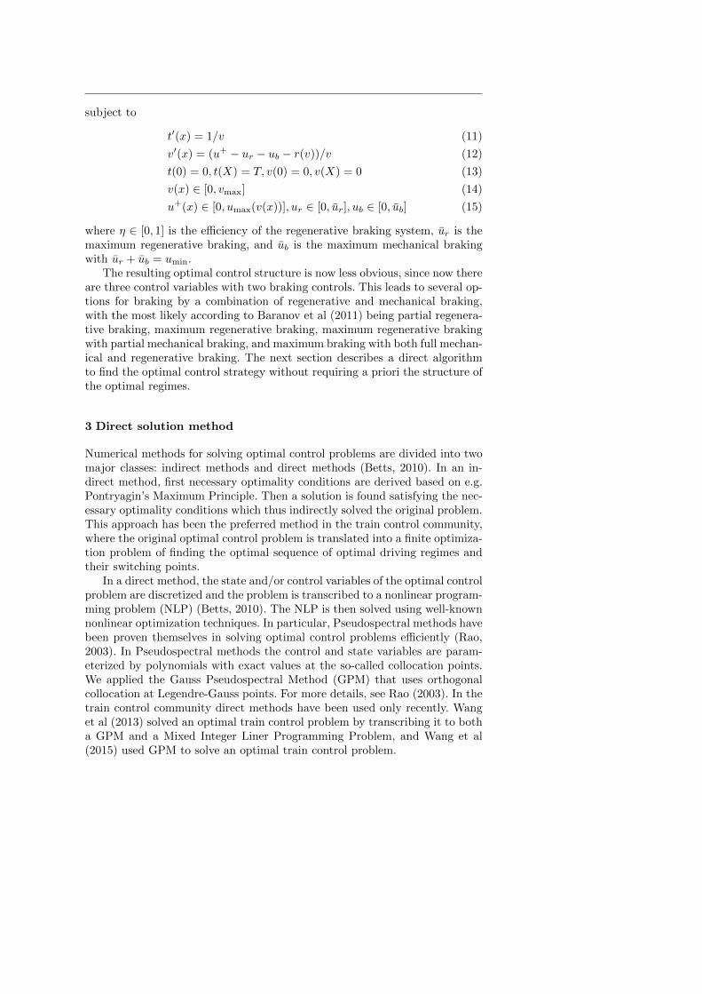
The model is applied between the stations Driebergen-Zeist (Db) andMaarn (Mrn) in the Netherlands, see figure 3. Only the direction of Db toMrn is considered in this paper. A local train of the Netherlands Railways(NS) (train series 7400) is running on this section stopping at both stations.The following data is available:

– Total distance between two stations is 7668 m.– Total available running time according to the timetable of 2015 is 6 min-

utes.– Maximum allowed speed at the section is 140 km/h.– Rolling stock type SLT-6 (Sprinter Light Train) of NS is running on this

section.

Fig. 3 Case study of local train series 7400 between Driebergen-Zeist and Maarn (insideblack dotted square)

Besides, the following assumptions are made for modelling the problem:

– Maximum service braking (brake step 4 of SLT) instead of maximum brak-ing is assumed for the the train, since this is more comfortable for thepassengers and the train conductor in the train.

– No varying gradient profile and curves are used in the model.– Signalling and ATP (Automatic Train Protection) system are not taken

into account.– Only the total traction energy consumption at the pantograph of a single

train is considered, so no transmission losses of the energy (like regeneratedenergy) are taken into account and no other surrounding trains are takeninto account.

The first step taken is to compare the model results generated by the EZ3Rmodel with the EZR model. This is done by comparing both the time-optimal(TO) or technical minimum running time (i.e. a running a train as fast aspossible from one station to the next station) and the energy-efficient traincontrol (EETC) of both models. The EZR model is already calibrated, vali-dated and verified and is in accordance with the results from optimal controltheory (Scheepmaker and Goverde, 2015). Therefore, if the EZ3R model re-sults are in line with the results of the EZR model, the EZ3R model is assumedto be plausible for further application.

The first important result of the model is that the calculation speed of theEZ3R model (5 s) is much faster than the the EZR model (122 s) (computedat a laptop with a 2.1 GHz processor and 8 GB RAM)).

Secondly, the model results are analyzed, which are visualized in figure4. The results show that in general the EZ3R model generates results whichare in line with the EZR model. However, the main differences exists in theenergy consumption. For TO the EZ3R model calculates 0.7% higher energyconsumption than the EZR model. For the EETC this is even higher, i.e. 2.5%.

Based on this analysis, it is concluded that the EZ3R model is a goodalternative to the EZR model and the model results are comparable. Therefore,the EZ3R model is extended by including regenerative braking (RB), in orderto investigate how RB will change the energy-efficient driving strategy. Threedifferent models are compared based on the rolling stock data of NS:

1. EETC with only MeB (mechanical braking).2. EETC with both MeB and regenerative braking (RB) (normal situation

for SLT trains of NS).3. EETC with only RB.

For the first two variants of the model, the total maximum braking forceis the same (285.8 kN). This is because the electro-dynamic brakes can alsobe applied if the train cannot apply the regenerated energy (burn the regener-ated energy as heat like mechanical braking). For the third variant, the totalmaximum braking force is less than the other variants (150 kN), since now themechanical brakes are not applied.

The model results in GPOPS are generated within 20 s for the differentbraking variants. The results are displayed in figure 5. From the graphs the

Fig. 4 Comparison of the time-optimal (TO) and energy-efficient train control (EETC)driving strategies between the EZ3R model and the EZR model (left speed-distance graphand right energy-distance graph)

effect of bang-bang control in GPOPS becomes clear for the driving strategiesincluding RB. The fluctuation is clearly visible during the cruising drivingregime. The traction control shows a lot of fluctuating peaks during this phase,which indicates that GPOPS has difficulties in calculating this bang-bangcontrol during cruising.

Moreover, the main differences between EETC with MeB or RB becomeclear in the figure. If only MeB is applied, the train is accelerating to a higherspeed than when RB is (also) applied. Secondly when RB is included, a cruisingphase with a lower maximum speed is applied compared to MB only. The speedat which braking starts with RB is also higher than with only MeB, since RBnow generates energy. It can be stated that the more energy that can begenerated by RB, the higher the speed at the beginning of the braking phasewill be. However, the maximum speed will always be lower than with MeBonly, since a cruising phase with a lower maximum speed is included with RB.

The differences between EETC with MeB & RB and only RB are minimum.The energy consumption of only RB is slightly higher (1%) which can beexplained by the fact that the available braking force with only RB is lowerthan combining both MeB and RB together. This means the train with onlyRB starts braking earlier and has a slightly higher cruising speed comparedto the braking strategy with MeB & RB.

The results indicate that energy savings of 29.5% can be achieved by com-bining MeB and RB in the EETC compared to EETC with only MeB. Theenergy savings with only RB are a slightly lower, i.e. 28.8%.

So it can be concluded that including regenerative braking in EETC hasa big influence on the extra decrease in total traction energy consumption.The effects of varying gradients (and varying speed limits) might even havea bigger effect on the total traction energy consumption for EETC with RB,since during downwards slopes RB can be applied to regenerate energy andabsorb the potential energy. This will be a topic for future research.

Fig. 5 Comparison between the energy-efficient train control (EETC) driving strategieswith only mechanical braking (MeB), both MeB and regenerative braking (RB) or only RBof the EZ3R model (left speed-distance graph and right energy-distance graph)

5 Conclusion

In this paper an optimal train control problem has been considered in whichtotal traction energy is minimized by including the effects of regenerative brak-ing (RB). To compare the different energy-efficient train control (EETC) driv-ing strategies with mechanical braking (MeB) and/or RB, an optimal controlproblem has been formulated and solved by the Gauss Pseudospectral Method.

The model has been applied in a case study in three scenarios: no regenera-tive braking, both regenerative and mechanical braking and only regenerativebraking. The regenerative braking on level track had an impact on the op-timal driving strategy. With regenerative braking the optimal cruising speedis lower than without, the coasting regime is shorter, and the braking regimestarts earlier. This led to an extra energy saving of at least 28%. Based on thisresearch the main conclusion is that regenerative braking does influence theenergy-efficient driving strategy and leads to lower energy consumption.

In future research the model will be extended to include varying gradientsand speed limits, as well as signalling constraints.

References

Asnis IA, Dmitruk AV, Osmolovskii NP (1985) Solution of the problem ofthe energetically optimal control of the motion of a train by the maximumprinciple. USSR Computational Mathematics and Mathematical Physics25(6):37–44, DOI http://dx.doi.org/10.1016/0041-5553(85)90006-0

Baranov LA, Meleshin IS, Chin’ LM (2011) Optimal control of a subway trainwith regard to the criteria of minimum energy consumption. Russian Elec-trical Engineering 82(8):405–410, DOI 10.3103/s1068371211080049

Betts JT (2010) Practical Methods for Optimal Control and Estimation UsingNonlinear Programming, 2nd edn. SIAM, Philadelphia, PA, USA

Davis W (1926) The tractive resistance of electric locomotives and cars. Gen-eral Electric Review 29(October)

Franke R, Terwiesch P, Meyer M (2000) An algorithm for the optimal control ofthe driving of trains. In: Proceedings of the 39th IEEE Conference on Deci-sion and Control, vol 3, pp 2123–2128 vol.3, DOI 10.1109/CDC.2000.914108

Howlett PG (1996) Optimal strategies for the control of a train. Automatica32(4):519–532, DOI 10.1016/0005-1098(95)00184-0

Khmelnitsky E (2000) On an optimal control problem of train operation. IEEETransactions on Automatic Control 45(7):1257–1266, DOI 10.1109/9.867018

Liu RR, Golovitcher IM (2003) Energy-efficient operation of rail vehicles.Transportation Research Part A: Policy and Practice 37(10):917–932, DOI10.1016/j.tra.2003.07.001

Pontryagin LS, Boltyanskii VG, Gamkrelidze RV, Misiichenko EF (1962) TheMathematical Theory of Optimal Processes. Interscience Publishers, NewYork, NY, USA

Qu J, Feng X, Wang Q (2014) Real-time trajectory planning for rail tran-sit train considering regenerative energy. In: IEEE 17th International Con-ference on Intelligent Transportation Systems (ITSC) 2014, pp 2738–2742,DOI 10.1109/ITSC.2014.6958128

Rao AV (2003) Extension of a pseudospectral legendre method to non-sequential multiple-phase optimal control problems. In: AIAA Guidance,Navigation, and Control Conference

Rao AV, Benson DA, Darby C, Patterson MA, Francolin C, Sanders I,Huntington GT (2010a) Algorithm 902: GPOPS, a MATLAB Software forSolving Multiple-Phase Optimal Control Problems Using the Gauss Pseu-dospectral Method. ACM Transactions on Mathematical Software (TOMS)37(2):22

Rao AV, Benson DA, Darby CL, Huntington GT (2010b) User’s Manuel forGPOPS Version 3.3: A MATLAB Solving for Solving Optimal Control Prob-lems Using Pseudospectral Methods. Report

Rodrigo E, Tapia S, Mera J, Soler M (2013) Optimizing Electric Rail EnergyConsumption Using the Lagrange Multiplier Technique. Journal of Trans-portation Engineering 139(3):321–329, DOI doi:10.1061/(ASCE)TE.1943-5436.0000483

Rump SM (1999) INTLAB INTerval LABoratory, Kluwer Academic Publish-ers, Dordrecht, The Netherlands, book section 7, pp 77–104

Scheepmaker GM, Goverde RMP (2015) Running time supplements: energy-efficient train control versus robust timetables. In: Proceedings 6th Inter-national Conference on Railway Operations Modelling and Analysis (Rail-Tokyo2015), Narashino, Japan, 23-26 March, 2015

Wang P, Goverde RMP, Ma L (2015) A multiple-phase train trajectory opti-mization method under real-time rail traffic management. In: 18th IEEE In-ternational Conference on Intelligent Transportation Systems (ITSC 2015),Las Palmas, September 15-18, 2015

Wang Y, De Schutter B, Van den Boom TJJ, Ning B (2013) Optimal trajectoryplanning for trains: A pseudospectral method and a mixed integer linearprogramming approach. Transportation Research Part C 29:97–114