delft university of technology identification of a cessna...

Delft University of Technology

Identification of a Cessna Citation II Model Based on Flight Test Data

van den Hoek, Marlon; de Visser, Coen; Pool, Daan

Publication date2017Document VersionAccepted author manuscriptPublished in4th CEAS Specialist Conference on Guidance, Navigation and Control

Citation (APA)van den Hoek, M., de Visser, C., & Pool, D. (2017). Identification of a Cessna Citation II Model Based onFlight Test Data. In 4th CEAS Specialist Conference on Guidance, Navigation and Control: Warsaw, Poland

Important noteTo cite this publication, please use the final published version (if applicable).Please check the document version above.

CopyrightOther than for strictly personal use, it is not permitted to download, forward or distribute the text or part of it, without the consentof the author(s) and/or copyright holder(s), unless the work is under an open content license such as Creative Commons.

Takedown policyPlease contact us and provide details if you believe this document breaches copyrights.We will remove access to the work immediately and investigate your claim.

This work is downloaded from Delft University of Technology.For technical reasons the number of authors shown on this cover page is limited to a maximum of 10.

Identification of a Cessna Citation II ModelBased on Flight Test Data

M.A. van den Hoek, C.C. de Visser , D.M. Pool

Abstract

As a result of new aviation legislation, from 2019 on all air-carrier pilots areobliged to go through flight simulator-based stall recoverytraining. For this reasonthe Control and Simulation division at Delft University of Technology has set upa task force to develop a new methodology for high-fidelity aircraft stall behav-ior modeling and simulation. As part of this research project, the development of anew high-fidelity Cessna II simulation model, valid throughout the normal, pre-stallflight envelope, is presented in this paper. From an extensive collection of flight testdata, aerodynamic model identification was performed usingthe Two-Step Method.New in this approach is the use of the Unscented Kalman Filterfor an improvedaccuracy and robustness of the state estimation step. Also,for the first time an ex-plicit data-driven model structure selection is presentedfor the Citation II by makinguse of an orthogonal regression scheme. This procedure has indicated that most ofthe six non-dimensional forces and moments can be parametrized sufficiently by alinear model structure. It was shown that only the translational and lateral aerody-namic force models would benefit from the addition of higher order terms, morespecifically the squared angle of attack and angle of sideslip. The newly identifiedaerodynamic model was implemented into an upgraded versionof the existing sim-ulation framework and will serve as a basis for the integration of a stall and post-stallmodel.

M.A. van den HoekDelft University of Technology, Delft, The Netherlands e-mail:[email protected]

C.C. de VisserDelft University of Technology, Delft, The Netherlands e-mail: [email protected]

D.M. PoolDelft University of Technology, Delft, The Netherlands e-mail: [email protected]

1

[email protected]

[email protected]

[email protected]

2 M.A. van den Hoek, C.C. de Visser , D.M. Pool

1 Introduction

A S a result of new aviation legislation, from 2019 on all air-carrier pilots areobliged to go through flight simulator-based stall recoverytraining [1]. This

implies that all aircraft dynamics models driving flight simulators must be updatedto include accurate pre-stall, stall, and post-stall dynamics. For this reason, the Con-trol and Simulation (C&S) division at Delft University of Technology has set upa task force to develop a new methodology for high-fidelity aircraft stall behaviormodeling and simulation. This research effort is twofold. First, the current simula-tion framework is to be updated together with the implementation of a newly devel-oped aerodynamic model identified from flight test data obtained from TU Delft’sCessna Citation II laboratory aircraft. As second part of this research effort, an aero-dynamic stall model for the Citation II based on flight test data will be developedand integrated into the upgraded simulation framework.

At this moment, the C&S division uses a simulation model of the Cessna Cita-tion I, known as the Delft University Aircraft Simulation Model and Analysis Tool(DASMAT)[2] as its baseline model. This simulation model was designed as stan-dard Flight CAD package for control and design purposes within the C&S divisionof the Faculty of Aerospace Engineering, Delft University of Technology. DASMATis known for a number of deficiencies; most significantly is its unsatisfactory matchwith the current laboratory aircrafts flight dynamics. The Citation I model is the re-sult of a flight test program executed for the development of mathematical modelsdescribing the aerodynamic forces and moments, engine performance characteris-tics, flight control systems and landing gear [3]. Earlier attempts at modeling thelongitudinal forces and the pitching moment were made by Oliveira et al.[4]. How-ever, parameter estimates were only obtained for a limited range of flight conditionswith a very limited set of measurements. In addition, in the same paper the authorsstate that dependency of the aerodynamic model from higher order terms, such asα2 and terms relating to the time rate of change of the aerodynamic angles, such asα, are yet to be investigated[4].

The estimation of stability and control derivatives from flight test data can beformulated in the framework of maximum likelihood estimation [5]. In the con-text of this paper, aerodynamic model identification will bedone by employing theTwo-Step Method (TSM)[6, 7]. This method effectively decomposes the non-linearmodel identification problem into a non-linear flight path reconstruction problemand linear parameter estimation problem, allowing the use of linear parameter es-timation techniques for a significant simplification of the latter procedure. This de-composition can be made under certain conditions concerning accuracy and typeof the in-flight measurements[7]. New to the TSM approach is the use of the Un-scented Kalman Filter[8] (UKF) for an improved accuracy and robustness of thestate estimates in the first step.

Identification of a Cessna Citation II Model Based on Flight Test Data 3

2 Research Vehicle and Flight Data

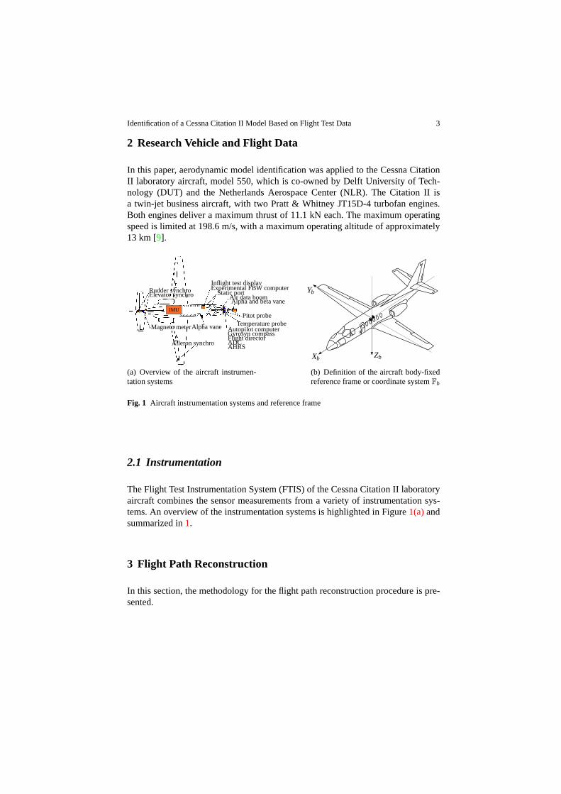
In this paper, aerodynamic model identification was appliedto the Cessna CitationII laboratory aircraft, model 550, which is co-owned by Delft University of Tech-nology (DUT) and the Netherlands Aerospace Center (NLR). The Citation II isa twin-jet business aircraft, with two Pratt & Whitney JT15D-4 turbofan engines.Both engines deliver a maximum thrust of 11.1 kN each. The maximum operatingspeed is limited at 198.6 m/s, with a maximum operating altitude of approximately13 km [9].

Inflight test display

Gyrosyn compassAutopilot computer

Aileron synchro

Rudder synchro

Magneto meter

Air data boom

Alpha vane

Alpha and beta vane

Pitot probe

Static portElevator synchroExperimental FBW computer

Temperature probe

Flight directorADCAHRS

IMU

(a) Overview of the aircraft instrumen-tation systems

ZbXb

Yb

(b) Definition of the aircraft body-fixedreference frame or coordinate systemFb

Fig. 1 Aircraft instrumentation systems and reference frame

2.1 Instrumentation

The Flight Test Instrumentation System (FTIS) of the CessnaCitation II laboratoryaircraft combines the sensor measurements from a variety ofinstrumentation sys-tems. An overview of the instrumentation systems is highlighted in Figure1(a)andsummarized in1.

3 Flight Path Reconstruction

In this section, the methodology for the flight path reconstruction procedure is pre-sented.


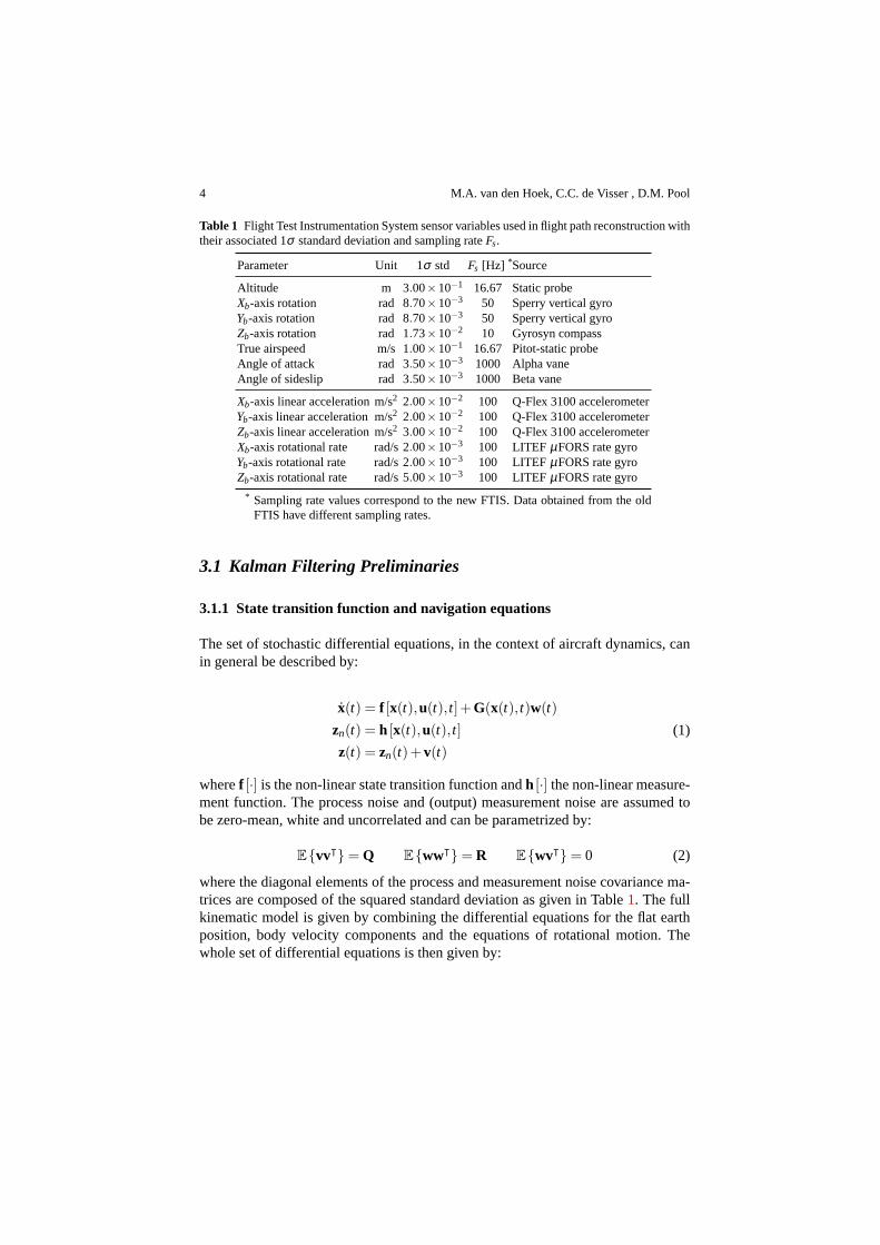
Table 1 Flight Test Instrumentation System sensor variables used in flight path reconstruction withtheir associated 1σ standard deviation and sampling rateFs.

Parameter Unit 1σ std Fs [Hz] *Source

Altitude m 3.00×10−1 16.67 Static probeXb-axis rotation rad 8.70×10−3 50 Sperry vertical gyroYb-axis rotation rad 8.70×10−3 50 Sperry vertical gyroZb-axis rotation rad 1.73×10−2 10 Gyrosyn compassTrue airspeed m/s 1.00×10−1 16.67 Pitot-static probeAngle of attack rad 3.50×10−3 1000 Alpha vaneAngle of sideslip rad 3.50×10−3 1000 Beta vane

Xb-axis linear acceleration m/s2 2.00×10−2 100 Q-Flex 3100 accelerometerYb-axis linear acceleration m/s2 2.00×10−2 100 Q-Flex 3100 accelerometerZb-axis linear acceleration m/s2 3.00×10−2 100 Q-Flex 3100 accelerometerXb-axis rotational rate rad/s 2.00×10−3 100 LITEFµFORS rate gyroYb-axis rotational rate rad/s 2.00×10−3 100 LITEFµFORS rate gyroZb-axis rotational rate rad/s 5.00×10−3 100 LITEFµFORS rate gyro

* Sampling rate values correspond to the new FTIS. Data obtainedfrom the oldFTIS have different sampling rates.

3.1 Kalman Filtering Preliminaries

3.1.1 State transition function and navigation equations

The set of stochastic differential equations, in the context of aircraft dynamics, canin general be described by:

x(t) = f [x(t),u(t), t]+G(x(t), t)w(t)

zn(t) = h [x(t),u(t), t]

z(t) = zn(t)+v(t)

(1)

wheref [·] is the non-linear state transition function andh [·] the non-linear measure-ment function. The process noise and (output) measurement noise are assumed tobe zero-mean, white and uncorrelated and can be parametrized by:

E{vv⊺}= Q E{ww⊺}= R E{wv⊺}= 0 (2)

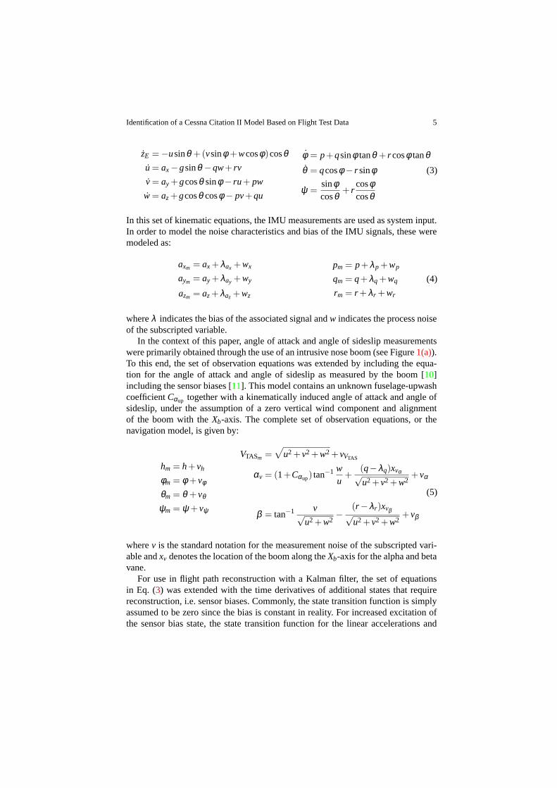
where the diagonal elements of the process and measurement noise covariance ma-trices are composed of the squared standard deviation as given in Table1. The fullkinematic model is given by combining the differential equations for the flat earthposition, body velocity components and the equations of rotational motion. Thewhole set of differential equations is then given by:


zE =−usinθ +(vsinφ +wcosφ)cosθu= ax−gsinθ −qw+ rv

v= ay+gcosθ sinφ − ru+ pw

w= az+gcosθ cosφ − pv+qu

φ = p+qsinφ tanθ + r cosφ tanθθ = qcosφ − r sinφ (3)

ψ =sinφcosθ

+ rcosφcosθ

In this set of kinematic equations, the IMU measurements areused as system input.In order to model the noise characteristics and bias of the IMU signals, these weremodeled as:

axm = ax+λax +wx

aym = ay+λay +wy

azm = az+λaz +wz

pm = p+λp+wp

qm = q+λq+wq (4)

rm = r +λr +wr

whereλ indicates the bias of the associated signal andw indicates the process noiseof the subscripted variable.

In the context of this paper, angle of attack and angle of sideslip measurementswere primarily obtained through the use of an intrusive noseboom (see Figure1(a)).To this end, the set of observation equations was extended byincluding the equa-tion for the angle of attack and angle of sideslip as measuredby the boom [10]including the sensor biases [11]. This model contains an unknown fuselage-upwashcoefficientCαup together with a kinematically induced angle of attack and angle ofsideslip, under the assumption of a zero vertical wind component and alignmentof the boom with theXb-axis. The complete set of observation equations, or thenavigation model, is given by:

hm = h+vh

φm = φ +vφ

θm = θ +vθ

ψm = ψ +vψ

VTASm =√

u2+v2+w2+vVTAS

αv = (1+Cαup) tan−1 wu+

(q−λq)xvα√u2+v2+w2

+vα

(5)

β = tan−1 v√u2+w2

−(r −λr)xvβ√u2+v2+w2

+vβ

wherev is the standard notation for the measurement noise of the subscripted vari-able andxv denotes the location of the boom along theXb-axis for the alpha and betavane.

For use in flight path reconstruction with a Kalman filter, theset of equationsin Eq. (3) was extended with the time derivatives of additional states that requirereconstruction, i.e. sensor biases. Commonly, the state transition function is simplyassumed to be zero since the bias is constant in reality. For increased excitation ofthe sensor bias state, the state transition function for thelinear accelerations and


fuselage-upwash coefficient was modeled as zero-mean unit-variance random walkscaled by a factork, as earlier applied in the work of Mulder et al.[12]:

λ ∼ k ·N (0,1) (6)

The bias state transition function for the rotational rateswas assumed to be zero forits usually very small bias. On balance, the state vector together with the augmentedbias terms is given by:

x =[

h u v wφ θ ψ λax λay λaz λp λq λr Cαup

]⊺(7)

3.2 Kalman Filtering Procedure

To begin with the formulation of the augmented UKF [8, 13, 14, 15], the augmentedstate vector and covariance matrix are defined as:

xa(k) = [x(k|k)⊺ v(k)⊺ w(k)⊺]⊺ (8)

Pa(k) =

P(k) 0 00 Q 00 0 R

(9)

wherev andw in the augmented state vector represent the means of the processand measurement noise; these can therefore be assumed to have zero mean, hencetheir values will be zero. The augmented state vector and covariance matrix can theneasily be transformed to the unscented domain by:

Xai (k) =

[

xa(k)+√

(L+λ )Pa(k)]

i = 1,2, . . . ,L

Xai (k) =

[

xa(k)−√

(L+λ )Pa(k)]

i = L+1,L+2, . . . ,2L(10)

This set of transformed points, indicated byXa, is referred to as the set of sigma

points. ParametersL and λ are, respectively, the dimensionality of the state vec-tor and a scaling factor defined asλ = α2(L+ κ)−L. α is a parameter to reflectthe spread of the sigma points around its mean, state vectorx, andβ is a factor toaccount for any prior knowledge. The latter is set to a value of 2 for Gaussian distri-butions.κ is an extra scaling factor which is usually set to zero. Subsequently, theweights for the set of transformed means and covariances aredefined as follows:


W(m)0 =

λL+λ

W(c)0 =

λL+λ

+(1−α2+β )

W(m)i =W(c)

i =1

2(L+λ )i = 1,2, . . . ,2L

(11)

From this point, the equations of the UKF become more trivial. Analogously tothe EKF, the state vector which is now expressed as sigma points are propagatedthrough the system’s dynamics:

Xa(k+1|k) = X

a (k|k)+∫ tk+1

tkf [X a,x(k|k),u(k),X a,v(k|k),τ ]dτ (12)

whereXa,x refers to the columns of the sigma points matrix related to the state and

superscriptv refers to the sigma points related to the process noise. The one stepahead state estimation can be calculated by:

x(k+1|k) =2L

∑i=0

W(m)i X

a (k+1|k) (13)

and the one step ahead covariance matrix by:

P(k+1|k) =2L

∑i=0

W(c)i

(

Xa,xi − x(k|k)

)(

Xa,xi − x(k|k)

)

⊺(14)

Again, similarly to the EKF, the sigma points representing the state vector andmeasurement noise are propagated through the measurement equations and subse-quently the transformed means for the measurements are calculated:

Y (k+1|k) = h [X a,x(k+1|k),X a,w(k+1|k)] (15)

with the transformed measurements given by taking the mean of the transformedsigma points:

y =2L

∑i=0

W(m)i Y i(k+1|k) (16)

The measurement covariance and measurement-state cross-covariance can becalculated by:

Pyy =2L

∑i=0

W(c)i (Y i(k+1|k)− y(k|k))(Y i(k+1|k)− y(k|k))⊺ (17)

Pxy =2L

∑i=0

W(c)i

(

Xa,xi − x(k|k)

)

(Y i − y(k|k))⊺ (18)


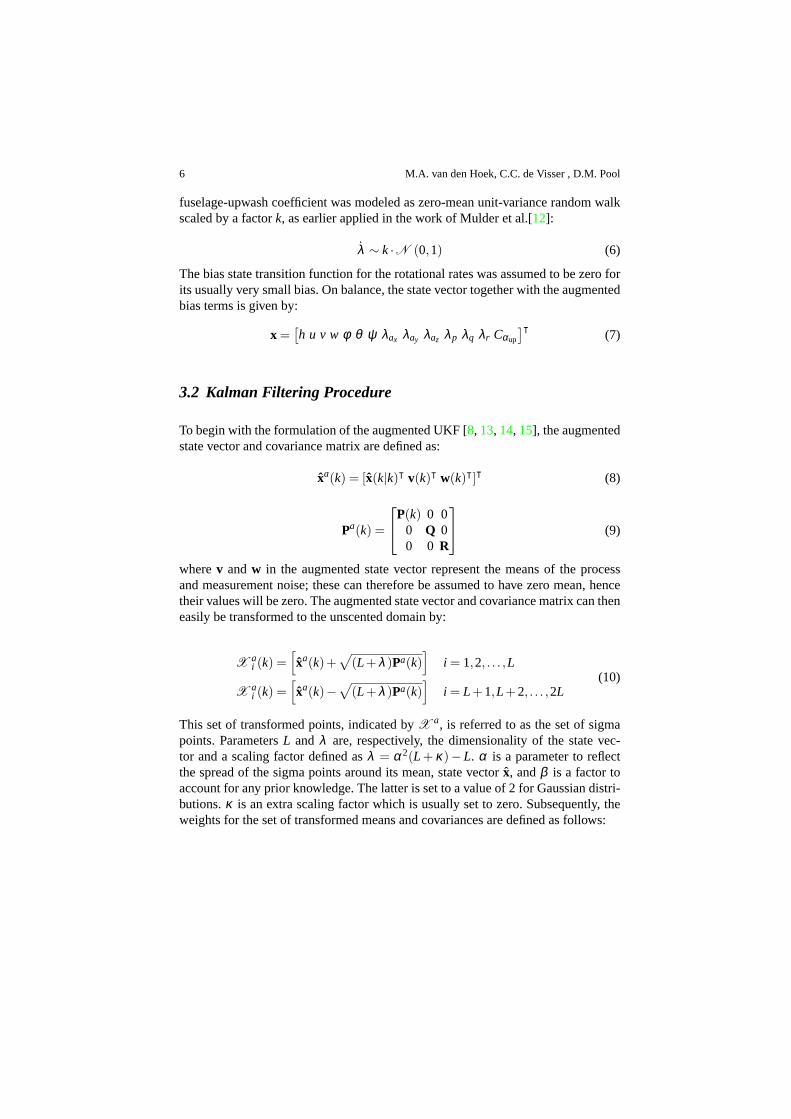
Finally, to complete the definition of the augmented UKF, gain matrixK , cor-rected state estimationx(k+ 1|k+ 1) and corrected covariance matrix estimationP(k+1|k+1) are expressed as:

K (k+1) = PxyP−1yy (19)

x(k+1|k+1) = x(k+1|k)+K {y(k+1)− y(k+1|k)} (20)

P(k+1|k+1) = P(k+1|k)−K (k+1)PyyK⊺(k+1) (21)

For additional numerical stability and guaranteed semi-definite state covariancematrix, the square-root implementation of the UKF can be used [16]. This type usesthe Cholesky decomposition to address certain numerical advantages in the calcula-tion of the transformed statistical properties. Further extensions to the UKF, e.g. theSigma-Point Kalman Filter [17] and its iterative counterpart [18] were introducedlater. However, these filters populate the whole state-space with sigma points insteadof only a selected optimal range. Therefore, the computational burden of such filtersdo not outweigh the advantages and their application is restricted [19].

4 Aerodynamic Model Identification

4.1 Preliminaries

The six non-dimensional forces and moments can be calculated by:

CX =m(ax−λax)−Tx

qS(22)

CY =m(

ay−λay

)

qS(23)

CZ =m(

ax−λaz

)

qS(24)

Cl =Ixx

qSb

(

p− Ixz

Ixx((p−λp)(q−λq)+ r)+

Izz− Iyy

Ixx(q−λq)(r −λr)

)

(25)

Cm =Iyy

qSc

(

q+Ixx− Izz

Iyy(p−λp)(r −λr)+

Ixz

Iyy

(

(p−λp)2− (r −λr)

2)

−MT

)

(26)


Cn =Izz

qSb

(

r − Ixz

Izz(p− (q−λq)(r −λr))+

Iyy− Ixx

Izz(p−λp)(q−λq)

)

(27)

whereλ denotes the bias obtained from the flight path reconstruction procedure foreach of the accelerations and rotational rates. Since the derivatives of the rotationalrates are not measured directly, these can be obtained by numerical differentiation.Corrections to the non-dimensional force inXb and the non-dimensional pitch ratewere made by making use of an engine model. The engine-produced thrust inZb

was neglected and assumed to be approximately zero.

4.2 Parameter Estimation

The principles of regression analysis are well known and previously applied in manydifferent researches in the framework of aerodynamic system identification [20, 21,22]. The ordinary least squares (OLS) estimator, defined as theminimum residual

ΘOLS = minΘ∈R

‖X ·Θ −y‖ (28)

where‖·‖ denotes theL2 norm in Euclidean spaceRn. The well-known solution interms of linear operations is given by:

Θ OLS = (X⊺X)−1X⊺y (29)

According to the Gauss-Markov theorem, the OLS estimator isthe best linearunbiased estimator under the assumption that the variance of the residuals should behomoscedastic and the correlation terms should vanish[23]. In addition, under theassumption of a normally distributed residuals vector the OLS estimator is identicalto the maximum likelihood estimator, effectively attaining the Cramer-Rao lowerbounds (CRLB)[24]. The standard bounds of the parameter estimates are given bythe diagonal elements of the variance-covariance matrix:

Cov{Θ}= E

{

(

Θ −Θ)⊺ (Θ −Θ

)

}

= σ2 (X⊺X)−1 (30)

whereσ2 can be approximated by the mean squared error of the residuals. Usingthe estimated covariance, pair-wise correlation of the estimated parameters can beassessed by:

Corr{

Θ}

=

1σ(Θ1)

0 . . . 0

0 1σ(Θ2)

. . . 0...

......

...0 0 . . .

1σ(Θp)

Cov{

Θ}

1σ(Θ1)

0 . . . 0

0 1σ(Θ2)

. . . 0...

..... .

...0 0 . . .

1σ(Θp)

(31)


Because aircraft parameter estimation is often associatedwith data collinearity[25],a biased parameter estimation technique known as PrincipalComponents Regres-sion (PRC) was used. PCR is able to increase the accuracy of the parameter esti-mates in case of multi-collinearity among the predictor variables [20].

4.3 Model Structure Selection

Stepwise regression[26] is a method specifically aimed at data-driven selection ofan appropriate model structure from a set of candidate regressors. Later modifi-cations to this approach restricted the selection of candidate regressors to higherorder terms, starting at a fixed linear model structure[27]. The pool of candidate re-gressors is to be formed by single terms, cross-interactions and higher order termscorresponding to the independent variables in the model. The downside of the step-wise regression method is that it includes addition and elimination criteria[28]. Inaddition, regressors cannot be evaluated independently because of their interactionwith other regressors in the selected model structure.

More recently, Morelli[21, 29] and Grauer[30] applied a multi-variate polyno-mial model obtained from an orthogonal model structure selection to various air-craft. The latter model structure selection technique transforms the full set of candi-date regressors to the orthogonal domain in order to test thesignificance of each pa-rameter. By defining a predicted square error (PSE)[30], selection of the orthogonalbasis functions can be done by minimization of the latter metric. Terms contributingless than a certain threshold value can also be removed from the model structure.

The process of orthogonal basis functions model structure selection begins withthe orthogonalization process of the set of candidate regressors:

p0 = 1, p j = x j −j−1

∑k=0

γk jpk for j = 1,2, . . . ,n (32)

wherex j is the j th vector of independent variables and coefficientγk j is defined as:

γk j =p⊺

kx j

p⊺

kpkfor k= 0,1, . . . , j −1 (33)

Orthogonal vectorsp0,p1, . . . ,pn now form the columns of orthogonal regressionmatrixP. The parameter estimate can now be obtained by the least squares estimatorin Eq. (29). This can be done by subsequently calculating the contribution to the totalleast-squares cost independently for each candidate regressor with:

J(a j) =

(

p⊺

j y)2

p⊺

j p j(34)

a selection can be made based on the PSE, which is defined as:


PSE=1N(y− y)⊺ (y− y)+σ2

maxnN

(35)

The maximum model fit error variance can be obtained from:

σ2max=

1N−1

N

∑i=1

(yi −y)2 (36)

5 Results

In this section the results of the flight path reconstruction, model structure selec-tion and parameter estimation procedure are presented. In addition, a comparisonbetween parameter estimates by Koehler and Hardover maneuvers is presented, fol-lowed by post identification smoothing of the locally identified models.

5.1 Flight Path Reconstruction

The results for the flight path reconstruction procedure comprises a total of morethan 200 individually reconstructed dynamic maneuvers, both longitudinally andlaterally induced. For this reason, only a selection of results is shown in this paper.For a typical 3-2-1-1 dynamic maneuver in elevator, the results are depicted in Fig-ure2. In this figure, the state estimate by the UKF together with the bias estimate,innovation sequences, filtered and reconstructed measurements and the control sur-face deflections during the maneuver are shown. Innovation sequences are shown toconfirm filter consistency.

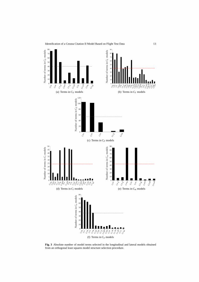
5.2 Aerodynamic Model Identification

The results from the model structure selection procedure and parameter estimationare presented in this section together with a model validation by applying the iden-tified least squares model to flight derived non-dimensionalforces and momentstogether with a comparison versus the currently implemented aerodynamic modelin the DASMAT simulation framework.

The final model structure of the non-dimensional forces and moments inXb, ob-tained from an orthogonal least squares model selection scheme, consisted of a totalof 5 terms, i.e.CX0, CXα , CXq, CXδe

, CXα2 . However, the term related to the squaredangle of attack was removed from the model for its high pairwise correlation withthe angle of attack term. Identified values for the parameters as tabulated in Table2.Tabulated values represent the parameters in the total number of locally identifiedmodels. The minimum, maximum and mean values for the estimated parameters


State estimate 2σ std bound

z[m

]

v[m

/s]

u[m

/s]

w[m

/s]

φ[r

ad]

ψ[r

ad]

θ[r

ad]

Time [s]0 10 20

0 10 200 10 200 10 20

0 10 200 10 200 10 20

1.72

1.74

1.76

0

0.1

0.2

-0.02

0

0.02

0.04

6

8

10

12

14

-2

-1

0

1

75

80

-5200

-5150

(a) UKF state estimate sequences

Bias estimate 2σ std bound

λ ay[m

/s2]

λ ax[m

/s2]

Cα u

p[r

ad]

λ az[m

/s2]

λ p[r

ad/s]

λ r[r

ad/s]

λ q[r

ad/s]

Time [s]0 10 20

0 10 200 10 200 10 20

0 10 200 10 200 10 20

0.2

0.25

0.3

-0.01

0

0.01

0.02

-6-4-202

×10−3

-5

0

5

×10−3

-1

-0.5

0

0.5

-2

-1

0

1

-0.5

0

0.5

1

(b) UKF bias estimate sequences

Innovation 2σ std bound

Time [s]

h[m

]ψ

[rad]

VTA

S[m

/s]

α[r

ad]

φ[r

ad]

θ[r

ad]

β[r

ad]

0 10 20

0 10 200 10 200 10 20

0 10 200 10 200 10 20

-0.02

0

0.02

-0.01

0

0.01

-0.5

0

0.5

-0.1

0

0.1

-0.04

-0.020

0.020.04

-0.04-0.02

0

0.020.04

-2

0

2

(d) UKF filter innovation sequences

Measurement Filtered Reconstructed

h[m

]

φ[r

ad]

θ[r

ad]

0 10 200 10 200 10 20

0

0.1

0.2

-0.02

0

0.02

0.04

5150

5200

Identification of a Cessna Citation II Model Based on Flight Test Data 13N

umbe

rof

term

sinC

Xm

odel

s

CX

0

CX

α

CX

α2

CX

αq

CX

q2

CX

qδe

CX

q

CX

αδ e

CX

δ e

CX

δ e20

10

20

30

40

50

60

70

80

(a) Terms inCX models

Num

ber

ofte

rms

inCY

mod

els

CY β

CY

pC

Y rC

Y βp

CY 0

CY

p2C

Y δ aC

Y β2

CY β

rC

Y δ rC

Ypδ

aC

Y βδ r

CY r

δ rC

Y βδ a

CY r2

CY

pr

CY

pδr

CY δ a

δ rC

Y δ r2

CY δ a

2C

Y rδ a

0

10

20

30

40

50

60

70

80

90

(b) Terms inCY models

Num

ber

ofte

rms

inCZ

mod

els

CZ

0

CZ

α

CZ

q

CZ

α2

CZ

δ e

0

20

40

60

80

100

120

(c) Terms inCZ models

Num

ber

ofte

rms

inCl

mod

els

Cl δ a

Cl β

pC

l pr

Cl p2

Cl δ r

Cl β

δ aC

l rC

l pδ a

Cl β

Cl p

Cl β

2C

l rδ a

Cl r2

Cl β

δ rC

l pδ r

Cl 0

Cl r

δ rC

l βr

Cl δ a

20

5

10

15

20

25

30

35

40

45

50

(d) Terms inCl models

Num

ber

ofte

rms

inCm

mod

els

Cm

α

Cm

q2

Cm

α2

Cm

δ e

Cm

0

Cm

q

Cm

δ e2

Cm

αq

Cm

q δe

Cm

αδ e

0

10

20

30

40

50

60

70

80

90

(e) Terms inCm models

Num

ber

ofte

rms

inCn

mod

els

Cn β

Cn r

Cn δ r

Cn

pC

n δ aC

n β2

Cn β

rC

np2

Cn β

δ aC

n βp

Cn

pr

Cn r

δ rC

n rδ a

Cn

pδr

Cn r2

Cn δ a

20

10

20

30

40

50

60

70

80

(f) Terms inCn models

Fig. 3 Absolute number of model terms selected in the longitudinal and lateral models obtainedfrom an orthogonal least squares model structure selection procedure.


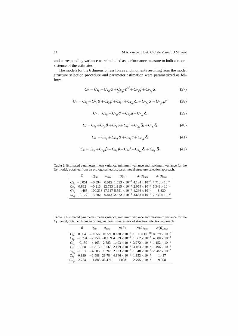
and corresponding variance were included as performance measure to indicate con-sistence of the estimates.

The models for the 6 dimensionless forces and moments resulting from the modelstructure selection procedure and parameter estimation were parametrized as fol-lows:

CX =CX0 +CXα α +✟✟✟✟CXα2 α2+CXqq+CXδe

δe (37)

CY =CY0 +CYβ β +CYp p+CYr r +CYδaδa+CYδr

δr +CYβ2 β 2 (38)

CZ =CZ0 +CZα α +CZqq+CZδeδe (39)

Cl =Cl0 +Clβ β +Clp p+Clr r +Clδaδa+Clδr

δr (40)

Cm =Cm0 +Cmα α +Cmqq+Cmδeδe (41)

Cn =Cn0 +Cnβ β +Cnp p+Cnr r +Cnδaδa+Cnδr

δr (42)

Table 2 Estimated parameters mean variance, minimum variance and maximum variance for theCX model, obtained from an orthogonal least squares model structureselection approach.

θ θmin θmax σ(θ) σ(θ)min σ(θ)max

CX0 −0.051 −0.594 0.019 1.553×10−5 4.134×10−8 4.710×10−4

CXα 0.862 −0.213 12.733 1.115×10−3 2.059×10−5 5.349×10−2

CXq −4.465−100.213 17.117 8.591×10−1 1.296×10−2 8.320CXδe

−0.172 −3.602 0.842 2.572×10−3 3.688×10−5 2.736×10−2

Table 3 Estimated parameters mean variance, minimum variance and maximum variance for theCY model, obtained from an orthogonal least squares model structureselection approach.


CY0 0.004 −0.056 0.059 8.638×10−8 3.190×10−10 8.079×10−7

CYβ −0.794 −2.258 −0.169 4.389×10−4 1.362×10−6 4.080×10−3

CYp −0.159 −4.163 2.583 1.403×10−2 3.772×10−5 1.152×10−1

CYr 1.958 −1.813 13.569 2.199×10−2 3.163×10−5 1.496×10−1

CYδa−0.180 −4.305 1.397 2.083×10−3 1.548×10−6 2.282×10−2

CYδr0.839 −1.988 26.784 4.846×10−2 1.152×10−6 1.427

CYβ2 2.754 −14.888 48.476 1.028 2.795×10−5 9.398


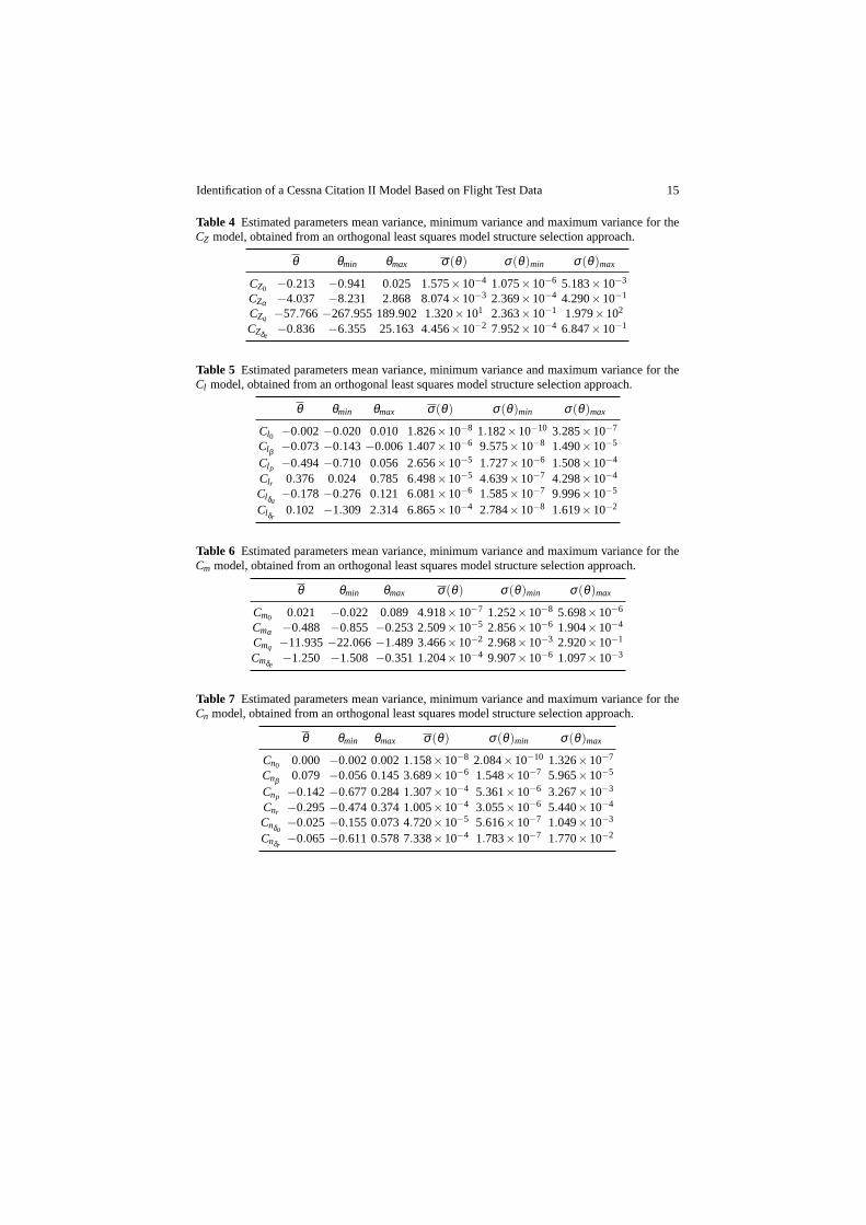
Table 4 Estimated parameters mean variance, minimum variance and maximum variance for theCZ model, obtained from an orthogonal least squares model structureselection approach.


CZ0 −0.213 −0.941 0.025 1.575×10−4 1.075×10−6 5.183×10−3

CZα −4.037 −8.231 2.868 8.074×10−3 2.369×10−4 4.290×10−1

CZq −57.766−267.955 189.902 1.320×101 2.363×10−1 1.979×102

CZδe−0.836 −6.355 25.163 4.456×10−2 7.952×10−4 6.847×10−1

Table 5 Estimated parameters mean variance, minimum variance and maximum variance for theCl model, obtained from an orthogonal least squares model structureselection approach.


Cl0 −0.002−0.020 0.010 1.826×10−8 1.182×10−10 3.285×10−7

Clβ −0.073−0.143−0.006 1.407×10−6 9.575×10−8 1.490×10−5

Clp −0.494−0.710 0.056 2.656×10−5 1.727×10−6 1.508×10−4

Clr 0.376 0.024 0.785 6.498×10−5 4.639×10−7 4.298×10−4

Clδa−0.178−0.276 0.121 6.081×10−6 1.585×10−7 9.996×10−5

Clδr0.102 −1.309 2.314 6.865×10−4 2.784×10−8 1.619×10−2

Table 6 Estimated parameters mean variance, minimum variance and maximum variance for theCm model, obtained from an orthogonal least squares model structureselection approach.


Cm0 0.021 −0.022 0.089 4.918×10−7 1.252×10−8 5.698×10−6

Cmα −0.488 −0.855 −0.253 2.509×10−5 2.856×10−6 1.904×10−4

Cmq −11.935−22.066−1.489 3.466×10−2 2.968×10−3 2.920×10−1

Cmδe−1.250 −1.508 −0.351 1.204×10−4 9.907×10−6 1.097×10−3

Table 7 Estimated parameters mean variance, minimum variance and maximum variance for theCn model, obtained from an orthogonal least squares model structureselection approach.


Cn0 0.000 −0.002 0.002 1.158×10−8 2.084×10−10 1.326×10−7

Cnβ 0.079 −0.056 0.145 3.689×10−6 1.548×10−7 5.965×10−5

Cnp −0.142−0.677 0.284 1.307×10−4 5.361×10−6 3.267×10−3

Cnr −0.295−0.474 0.374 1.005×10−4 3.055×10−6 5.440×10−4

Cnδa−0.025−0.155 0.073 4.720×10−5 5.616×10−7 1.049×10−3

Cnδr−0.065−0.611 0.578 7.338×10−4 1.783×10−7 1.770×10−2


5.3 Model Validation

The identified models for all six non-dimensional forces andmoments were ap-plied to an independent validation data set consisting of 20% of the total data set.A comparison between the aircraft derived forces and moments, the least squaresmodel and the DASMAT model which is currently implemented inthe simulationframework is shown in Figure4. In addition, fit statistics in terms of the coefficientof determination and the relative root mean square error (RRMSE) are tabulated inTable8.

A time-domain comparison between the new least-squares model and DASMATfor a longitudinally induced 3-2-1-1 maneuver is presentedin Figure5. This fig-ure indicates an increased fidelity of the predicted aircraft states by the new least-squares model in comparison to the DASMAT model. Most significant is the betterfit of the new model for the velocity in the direction of theXb axis and the Eulerangles.

Table 8 Fit statistics for the least squares model and the existing DASMAT (D) model averagedover all validation sets.

CX CY CZ Cl Cm Cn

R2 0.76 0.77 0.77 0.75 0.76 0.85R2

D 0.60 0.55 0.64 0.25 0.00 0.50

RRMSE(%) 6.76 5.32 6.38 4.96 5.8 4.72RRMSED (%) 8.79 7.34 7.97 8.65 12.65 8.50

6 Conclusion

In this paper, the methodology regarding the identificationof an aerodynamic modelfor flight simulation training from flight test data was developed for the normal post-stall flight envelope. By employing the Two-Step Method (TSM), the UnscentedKalman Filter (UKF) was used in cooperation with linear parameter estimation tech-niques. Results indicate that the state estimates and measurement reconstructions bythe UKF are in good agreement with the presented data.

This research effort results in a simple and parsimonious set of aerodynamicmodels describing the 6 non-dimensional forces and moments. The model presentedin this paper outperforms the current aerodynamic model implemented in the DAS-MAT framework in terms of goodness of fit, in all 6 degrees of freedom, whencompared to the recorded forces and moments of the Cessna Citation II laboratoryaircraft. The explained variance of the non-dimensional forces was increased withat least 13%. More significant improvements were made to the non-dimensionalmoments; an increase of the explained variance of at least 35% was achieved.


Flight data Model fit DASMAT

Sample [k]

Mag

nitu

de[-

]

1.45 1.5 1.55

×1040.66 0.7 0.74

×1040.05 0.1 0.15

×104

0 0.5 1 1.5 2 2.5

×104

0

0.02

0.04

0.06

0

0.05

0.1

0.15

0

0.1

0.2

0

0.1

0.2

(a) IdentifiedCX model applied to a validation set

Sample [k]

Mag

nitu

de[-

]

6 6.1 6.2

×1043.8 4 4.2

×1041.6 1.8

×104

0 1 2 3 4 5 6 7

×104

-0.1

0

0.1

-0.02

0

0.02

-0.02

0

0.02

0.04

-0.1

0

0.1

(b) IdentifiedCY model applied to a validation set

Mag

nitu

de[-

]

Sample [k]

5.56 5.6 5.64

×1042.4 2.45 2.5 2.55

×1040.6 0.7 0.8

×104

0 1 2 3 4 5 6 7 8

×104

-0.8

-0.6

-0.4

-0.2

0

-1

-0.5

0

-0.8

-0.6

-0.4

-1.5

-1

-0.5

0

(c) IdentifiedCZ model applied to a validation set

Mag

nitu

de[-

]

Sample [k]

3.3 3.4×1042.3 2.35 2.4

×1040.6 0.7 0.8

×104

0 0.5 1 1.5 2 2.5 3 3.5 4 4.5

×104

-0.02

0

0.02

-0.02

0

0.02

-10

-5

0

5

×10−3

-0.02

0

0.02


Flight data Model fit DASMATr

[rad

/s]

q[r

ad/s

]

p[r

ad/s

]

w[m

/s]

u[m

/s]

v[m

/s]

Time [s]

δ r[d

eg]

δ e[d

eg]

δ a[d

eg]

ψ[r

ad]

φ[r

ad]

θ[r

ad]

2 4 6 8 2 4 6 8

2 4 6 8 2 4 6 8

2 4 6 8 2 4 6 8

2 4 6 8 2 4 6 8

2 4 6 8 2 4 6 8

2 4 6 8 2 4 6 8

-0.10

0.1

-0.20

0.2

-0.10

0.1

95100105110

-8-404

-100

1020

-0.20

0.2

0.10.20.3

0.4

0.6

-0.40

0.4

-4-2024

-0.050

0.050.1

Fig. 5 Time domain response of the newly implemented aerodynamic model together with thecurrently implemented aerodynamic model in the DASMAT simulationframework and the flightderived aircraft states and control surface deflections for a longitudinally inducedδe 3-2-1-1 ma-neuver.

The work presented in this paper will serve as a basis for the integration of astall and post-stall model, resulting from a parallel research effort. Together, thesemodels will be used in future research into, e.g., the behavior of pilots during aero-dynamic stall and the development of new control algorithms.


References

1. Federal Aviation Administration, “Qualification, Service, and Use of Crewmembers and Air-craft Dispatchers,” Tech. rep., U.S. Department of Transportation, 2013.

2. van der Linden, C. A. A. M.,DASMAT - Delft University Aircraft Simulation Model andAnalysis Tool, Delft University Press, Delft, 1998.

3. Mulder, J. A., Baarspul, M., Breeman, J. H., Nieuwpoort, A. M. H., Verbaak, J. P. F., andSteeman, P. S. J. M., “Determination of the mathematical model for the new Dutch governmentcivil aviation flying school flight simulator,”Society of Flight Test Engineers, 18th Annualsymposium, Delft University of Technology, Amsterdam, 1987.

4. Oliveira, J., Chu, Q. P., Mulder, J. A., Balini, H. M. N. K., and Vos, W. G. M., “Output errormethod and two step method for aerodynamic model identification,”AIAA Guidance, Naviga-tion, and Control Conference and Exhibit, , No. August, 2005, pp. 1–9.

5. Nahi, N. E.,Estimation theory and applications, John Wiley & Sons, New York, 1969.6. Mulder, J. A., Chu, Q. P., Sridhar, J. K., Breeman, J. H., and Laban, M., “Non-linear aircraft

flight path reconstruction review and new advances,”Progress in Aerospace Sciences, Vol. 35,No. 7, 1999, pp. 673–726.

7. Mulder, J. A., Sridhar, J. K., and Breeman, J. H.,Identification of Dynamic Systems- Appli-cations to Aircraft Part 2: Nonlinear Analysis and Manoeuvre Design, Vol. 3, North AtlanticTreaty Organisation, Neuilly Sur Seine, 1994.

8. Julier, S. J. and Uhlmann, J. K., “A New Extension of the Kalman Filter to Nonlinear Sys-tems,” International Symposium for Aerospace Defense Sensing Simulutation and Controls,Vol. 3, No. 2, 1997, pp. 26.

9. Cessna Aircraft Company, “Operating Manual Model 550 Citation II, Unit -0627 And On,”Tech. rep., Wichita, Kansas, USA, 1990.

10. Laban, M.,On-Line Aircraft Aerodynamic Model Identification, Ph.d. thesis, Delft Universityof Technology, Delft, 1994.

11. de Visser, C. C.,Global Nonlinear Model Identification with Multivariate Splines, Ph.D. the-sis, Delft University of Technology, Delft, 2011.

12. Mulder, M., Lubbers, B., Zaal, P. M. T., van Paassen, M. M., and Mulder, J. A., “AerodynamicHinge Moment Coefficient Estimation Using Automatic Fly-by-WireControl Inputs,”Pro-ceedings of the AIAA Modeling and Simulation Technologies Conference and Exhibit, Chicago(IL), No. AIAA-2009-5692, 2009.

13. Chowdhary, G. and Jategaonkar, R., “Aerodynamic parameterestimation from flight data ap-plying extended and unscented Kalman filter,”Aerospace Science and Technology, Vol. 14,No. 2, 2010, pp. 106–117.

14. Julier, S. J. and Uhlmann, J. K., “Unscented filtering and nonlinear estimation,”Proceedingsof the IEEE, Vol. 92, No. 3, 2004, pp. 401–422.

15. Wan, E. A. and Van Der Merwe, R., “The unscented Kalman filterfor nonlinear estimation,”Adaptive Systems for Signal Processing, Communications, and Control Symposium 2000. AS-SPCC. The IEEE 2000, 2002, pp. 153–158.

16. Van Der Merwe, R. and Wan, E. A., “The square-root unscentedKalman filter for stateand parameter-estimation,”Acoustics, Speech, and Signal Processing, 2001. Proceedings.(ICASSP ’01). 2001 IEEE International Conference on, Vol. 6, 2001, pp. 3461–3464 vol.6.

17. van der Merwe, R. and Wan, E. A., “Sigma-Point Kalman Filters for Integrated Navigation,”Proceedings of the 60th Annual Meeting of the Institute of Navigation (ION), 2004, pp. 641–654.

18. Sibley, G., Sukhatme, G. S., and Matthies, L. H., “The Iterated Sigma Point Kalman Filterwith Applications to Long Range Stereo,”Rss, 2006.

19. Armesto, L., Tornero, J., and Vincze, M., “On multi-rate fusion for non-linear sampled-datasystems: Application to a 6D tracking system,”Robotics and Autonomous Systems, Vol. 56,No. 8, 2008, pp. 706–715.


20. Klein, V., “Estimation of aircraft aerodynamic parameters from flight data,” Progress inAerospace Sciences, Vol. 26, No. 1, 1989, pp. 1–77.

21. Morelli, E. A., “Global nonlinear parametric modelling with application to F-16 aerodynam-ics,” American Control Conference, 1998. Proceedings of the 1998, Vol. 2, jun 1998, pp. 997–1001 vol.2.

22. Morelli, E. and Derry, S. D., “Aerodynamic Parameter Estimation for the X-43A (Hyper-X)from Flight Data,”AIAA Atmosperic FlightMechanics Conference and Exhibit, , No. August,2005.

23. Goldberg, M. A. and Cho, H. A.,Introduction to Regression Analysis, WIT Press, Southamp-ton, UK, 2003.

24. Watson, P. K. and Teelucksingh, S. S.,A Practical Introduction to Econometric Methods:Classical and Modern, University of the West Indies Press, 2002.

25. Morelli, E. A., “Practical Aspects of the Equation-ErrorMethod for Aircraft Parameter Esti-mation,”AIAA Atmospheric Flight Mechanics Conference, , No. 6114, 2006, pp. 1–18.

26. Batterson, J. G. and Klein, V., “Partitioning of flight datafor aerodynamic modeling of aircraftat high angles of attack,”Journal of Aircraft, Vol. 26, No. 4, apr 1989, pp. 334–339.

27. Klein, V., Batterson, J. G., and Murphy, P. C., “Determination of airplane model structurefrom flight data by using modified stepwise regression,” Tech. rep.,NASA Langley ResearchCenter, Hampton, 1981.

28. Lombaerts, T., Oort, E. V., Chu, Q. P., Mulder, J. A., and Joosten, D., “Online AerodynamicModel Structure Selection and Parameter Estimation for Fault Tolerant Control,”Journal ofGuidance, Control, and Dynamics, Vol. 33, No. 3, 2010, pp. 707–723.

29. Morelli, E., “Efficient Global Aerodynamic Modeling fromFlight Data,” 50th AIAAAerospace Sciences Meeting including the New Horizons Forum andAerospace Exposition,Aerospace Sciences Meetings, American Institute of Aeronautics and Astronautics, jan 2012.

30. Grauer, J. A. and Morelli, E. A., “Generic Global Aerodynamic Model for Aircraft,” Journalof Aircraft, Vol. 52, No. 1, jul 2014, pp. 13–20.

delft university of technology identification of a cessna...

Documents