deliverable 2.1 v2 1 8 14 - eclipse.nilu.noeclipse.nilu.no/portals/83/project...

ECLIPSE Deliverable 2.1 1

Collaborative Project

Work Programme: Climate Forcing of non-UNFCCC gases, aerosols and black carbon Activity code: ENV.2011.1.1.2-2

Coordinator: Andreas Stohl, NILU – Norsk Institutt for Luftforskning

Start date of project: 1st November 2011

Duration: 36 months

Deliverable D2.1

Report on model accuracy

Due date of deliverable: Project month 24

Actual submission date: Project month 39

Organisation name of lead contributor for this deliverable: MET.NO

Authors/Contributors: MET.NO: Michael Schulz, Dirk Olivié, Svetlana Tsyro, FORTH: Maria Kanakidou, Stelios Myriokefalitakis, Nikos Daskalakis, Ulas Im, Georgios Fanourgakis CICERO: Øivind Hodnebrog, Ragnhild Skeie, Marianne Lund; Gunnar Myhre; METOFFICE: Nicolas Bellouin, Steven Rumbold, Bill Collins, ULEI: Ribu Cherian, Johannes Quaas


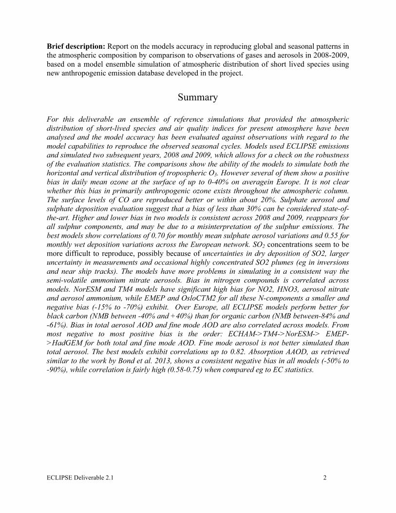
Brief description: Report on the models accuracy in reproducing global and seasonal patterns in the atmospheric composition by comparison to observations of gases and aerosols in 2008-2009, based on a model ensemble simulation of atmospheric distribution of short lived species using new anthropogenic emission database developed in the project.

Summary

For this deliverable an ensemble of reference simulations that provided the atmospheric distribution of short-lived species and air quality indices for present atmosphere have been analysed and the model accuracy has been evaluated against observations with regard to the model capabilities to reproduce the observed seasonal cycles. Models used ECLIPSE emissions and simulated two subsequent years, 2008 and 2009, which allows for a check on the robustness of the evaluation statistics. The comparisons show the ability of the models to simulate both the horizontal and vertical distribution of tropospheric O3. However several of them show a positive bias in daily mean ozone at the surface of up to 0-40% on averagein Europe. It is not clear whether this bias in primarily anthropogenic ozone exists throughout the atmospheric column. The surface levels of CO are reproduced better or within about 20%. Sulphate aerosol and sulphate deposition evaluation suggest that a bias of less than 30% can be considered state-of-the-art. Higher and lower bias in two models is consistent across 2008 and 2009, reappears for all sulphur components, and may be due to a misinterpretation of the sulphur emissions. The best models show correlations of 0.70 for monthly mean sulphate aerosol variations and 0.55 for monthly wet deposition variations across the European network. SO2 concentrations seem to be more difficult to reproduce, possibly because of uncertainties in dry deposition of SO2, larger uncertainty in measurements and occasional highly concentrated SO2 plumes (eg in inversions and near ship tracks). The models have more problems in simulating in a consistent way the semi-volatile ammonium nitrate aerosols. Bias in nitrogen compounds is correlated across models. NorESM and TM4 models have significant high bias for NO2, HNO3, aerosol nitrate and aerosol ammonium, while EMEP and OsloCTM2 for all these N-components a smaller and negative bias (-15% to -70%) exhibit. Over Europe, all ECLIPSE models perform better for black carbon (NMB between -40% and +40%) than for organic carbon (NMB between-84% and -61%). Bias in total aerosol AOD and fine mode AOD are also correlated across models. From most negative to most positive bias is the order: ECHAM->TM4->NorESM-> EMEP->HadGEM for both total and fine mode AOD. Fine mode aerosol is not better simulated than total aerosol. The best models exhibit correlations up to 0.82. Absorption AAOD, as retrieved similar to the work by Bond et al. 2013, shows a consistent negative bias in all models (-50% to -90%), while correlation is fairly high (0.58-0.75) when compared eg to EC statistics.


Contents Introduction ..................................................................................................................................... 4 Model Evaluation Methodology ..................................................................................................... 4 Results ............................................................................................................................................. 7

Ozone comparisons at surface –global ....................................................................................... 7 Ozone comparisons over Europe. ............................................................................................... 9 Carbon monoxide – global ........................................................................................................ 13 Model evaluation statistics for CO over Europe ....................................................................... 15 NO2 and HNO3 over Europe ..................................................................................................... 16 Sulfur dioxide over Europe ....................................................................................................... 17 Sulfate aerosols over Europe .................................................................................................... 18 Nitrogen containing aerosol components .................................................................................. 19

Nitrate aerosol ....................................................................................................................... 19 Ammonium aerosol ............................................................................................................... 20

Carbonaceous aerosols .............................................................................................................. 21 Particulate Organic Carbon ................................................................................................... 21 Black carbon ......................................................................................................................... 23

Coarse and fine aerosols ........................................................................................................... 24 Aerosol Optical Depth .............................................................................................................. 26

ECLIPSE Publications .................................................................................................................. 27 APPENDIX: List of stations over Europe used for the model evaluation. ................................... 28


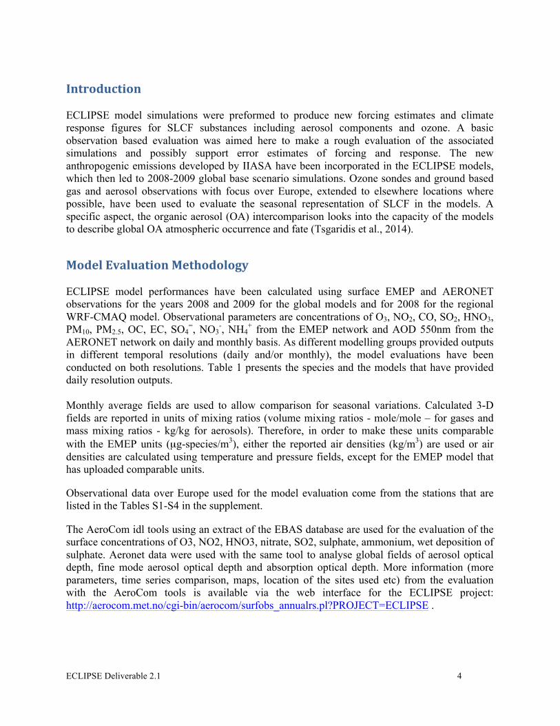
Introduction ECLIPSE model simulations were preformed to produce new forcing estimates and climate response figures for SLCF substances including aerosol components and ozone. A basic observation based evaluation was aimed here to make a rough evaluation of the associated simulations and possibly support error estimates of forcing and response. The new anthropogenic emissions developed by IIASA have been incorporated in the ECLIPSE models, which then led to 2008-2009 global base scenario simulations. Ozone sondes and ground based gas and aerosol observations with focus over Europe, extended to elsewhere locations where possible, have been used to evaluate the seasonal representation of SLCF in the models. A specific aspect, the organic aerosol (OA) intercomparison looks into the capacity of the models to describe global OA atmospheric occurrence and fate (Tsgaridis et al., 2014).

Model Evaluation Methodology ECLIPSE model performances have been calculated using surface EMEP and AERONET observations for the years 2008 and 2009 for the global models and for 2008 for the regional WRF-CMAQ model. Observational parameters are concentrations of O3, NO2, CO, SO2, HNO3, PM10, PM2.5, OC, EC, SO4

=, NO3-, NH4

+ from the EMEP network and AOD 550nm from the AERONET network on daily and monthly basis. As different modelling groups provided outputs in different temporal resolutions (daily and/or monthly), the model evaluations have been conducted on both resolutions. Table 1 presents the species and the models that have provided daily resolution outputs. Monthly average fields are used to allow comparison for seasonal variations. Calculated 3-D fields are reported in units of mixing ratios (volume mixing ratios - mole/mole – for gases and mass mixing ratios - kg/kg for aerosols). Therefore, in order to make these units comparable with the EMEP units (µg-species/m3), either the reported air densities (kg/m3) are used or air densities are calculated using temperature and pressure fields, except for the EMEP model that has uploaded comparable units.

Observational data over Europe used for the model evaluation come from the stations that are listed in the Tables S1-S4 in the supplement.

The AeroCom idl tools using an extract of the EBAS database are used for the evaluation of the surface concentrations of O3, NO2, HNO3, nitrate, SO2, sulphate, ammonium, wet deposition of sulphate. Aeronet data were used with the same tool to analyse global fields of aerosol optical depth, fine mode aerosol optical depth and absorption optical depth. More information (more parameters, time series comparison, maps, location of the sites used etc) from the evaluation with the AeroCom tools is available via the web interface for the ECLIPSE project: http://aerocom.met.no/cgi-bin/aerocom/surfobs_annualrs.pl?PROJECT=ECLIPSE .


The evaluations are based on statistical parameters of correlation coefficient (r), normalised mean bias (NMB), root mean square error (RMSE), and normalised mean error (NME).

( )( )

⎥⎥⎥⎥

⎦

⎤

⎢⎢⎢⎢

⎣

⎡−−

=∑=

PO

N

iii PPOO

Nrσσ

1

1

(Eq. 1)

( )100

1

1 ×−

=

∑

∑

=

=N

ii

N

iii

O

OMNMB (Eq. 2)

(Eq. 3)

100

1

1 ×−

=

∑

∑

=

=N

ii

N

iii

O

OMNME

(Eq. 4)

Table 1. Species provided by each model based on the temporal resolution Species ECHAM6-

HAM2 EMEP OsloCTM2 NorESM TM4-

ECPL WRF-

CMAQ Daily Monthly Daily Monthly Daily Monthly Daily Monthly Daily Monthly Daily Monthly

O3 ! ! ! ! ! ! ! ! NO2 ! ! ! ! ! ! ! ! CO ! ! ! ! ! SO2 ! ! ! ! ! ! ! HNO3 ! ! ! ! ! ! PM10 ! ! ! ! PM2.5 ! !* !* ! SO4

= ! ! ! ! ! ! ! ! NO3

- ! ! ! ! ! NH4

+ ! ! ! ! ! ! OC !# !# ! !$ ! ! ! EC ! ! ! ! ! ! ! AOD ! ! ! ! ! !

(*) calculated is the sum of all aerosol components except coarse mode sea-salt and dust.

( )∑=

−=N

iii OP

NRMSE

1

21


(#) provided as OM and converted to OC with a factor of OM/OC=1.4 (Tsigaridis et al., ACPD, 2014) ($) provided as OM and converted to OC with a factor of OM/OC as suggested by Dirk Olivie


Results

Ozone comparisons at surface –global ECLIPSE Global (TM4-ECPL, NORESM, EMEP and OsloCTM2) models are evaluated against O3 surface observations compiled from the European Monitoring and Evaluation Program (EMEP; http://www.emep.int/) and the World Ozone and Ultraviolet Radiation Data Centre (WOUDC; http://www.woudc.org), for the year 2008.

Figure 1 below shows the comparison of ECLIPSE monthly mean surface O3 simulations with the O3 observations (from EMEP and WDCGG database) for 2008 (left) and 2009 (right). These scatter plots show all annual mean data at all stations for the 4 global models TM4-ECPL, NORESM, EMEP and OsloCTM2 that reported O3 levels. The panels in Figure 2 show the month-by-month comparisons for the 4 models at several of the studied locations. TM4-ECPL and NORESM slightly overestimate surface O3, EMEP shows a good performance, OsloCTM2 slightly underestimates ozone. Seasonal cycles and summer maxima seem to be overestimated eg in Southern Europe by the NorESM and TM4-EPCL.

Figure 1. Comparison of monthly model results with observations of surface O3 at all available surface stations. TM4-ECPL: green, NorESM: blue, EMEP: red, OsloCTM2: cyan.


Figure 2. Comparison of model results with observations of surface O3 based on monthly mean values. Monthly mean observations using EBAS and WOUDC databases are marked with symbols with standard deviation (year 2008). TM4-ECPL: red, NorESM: green, EMEP: blue, OsloCTM2: yellow.


Ozone comparisons over Europe. Regarding O3 almost all ECLIPSE models (Figure 3) have similar temporal variation performances (r=~0.5-0.7). The statistics listed in Table 2 indicate that all ECLIPSE models reproduce reasonably well the surface O3 levels over Europe. EMEP global model and WRF-CMAQ mesoscale model are those performing the best with regard to the temporal variability of observed surface O3 over Europe.

Figure 3. Comparison of model results with observations of surface O3 (ug/m3) based on monthly mean values. Monthly mean observations using EBAS and WOUDC databases are marked with symbols with standard deviation. Coloured lines show model results as explained in the figure’s legend. Please note difference in colours from earlier figures. Table 2. Mean correlation coefficient (r), normalised mean bias (NMB), and root mean square error (RMSE) values calculated for O3 for each model on monthly resolution for 2008 and 2009, respectively. The statistics refer to the AeroCom evaluation over Europe (see sites and time series via AeroCom interface for ECLIPSE).

O3 R NMB (%) RMSE (ug/m3) 2008 2009 2008 2009 2008 2009

EMEP 0.82 0.82 18 17 7.8 7.4 OsloCTM2 0.71 0.71 0 0 6.6 6.3 NorESM 0.73 0.77 43 44 15.3 15.1

TM4-ECPL 0.69 0.70 30 29 12.7 12.5


Furthermore, the seasonality in the vertical structure of O3 calculated by the TM4-ECPLhas been evaluated by comparison with O3 sonde data from sites around the world, as provided by the WOUDC (Myriokefalitakis et al., in preparation). To compare with the seasonal variation as recorded from the ozonesonde observations both the model results and the O3 observations have been first interpolated into layers of 50 hPa from surface to the top of the atmosphere. Figure 3b below shows these comparisons over Europe and demonstrates the good model performance.

Figure 3b. Comparison of O3 levels (ppbv) from TM4-ECPL base simulation (red lines) with O3 sonde station data at five pressure levels (900-800-500-400-200 hPa) for six (WOUDC) stations: a) Hohenpeissenberg, Germany (47N, 11E); b) Payerne, Switzerland (46N, 6E)).


Figure 3b cont. as Fig 3 for c) De Bilt, Netherlands (52N, 5E); d) Ankara, Turkey (39N, 32E).


Figure 3b cont. as Fig. 3 for e) Lindenberg, Germany (52N, 14E); f) Legionowo, Poland (52N, 20E) To evaluate the model results in the troposphere, TM4-ECPL results for O3 (Figure 4a,b) and CO (Figure 6b,c) have been also compared with the Tropospheric Emission Spectrometer (TES)


satellite. TES is a high resolution (0.1 cm−1), infrared, Fourier Transform spectrometer aboard the NASA Aura satellite follows a polar Sun – synchronous orbit with an equator crossing time at 01:45 and 13:45 local time and has a repeat cycle of 16 days. In this study we use the version 4 of TES global survey data focusing on the relatively sensitive in the vertical region of 800–400 hPa). The TES products are provided in 67 levels in vertical with a varying layer thickness with an averaged nadir footprint of ~5 km by ~8 km (Beer et al., 2001). In order to compare TM4-ECPL model results with the TES observations, we sample the 3 – hourly model outputs at the times and locations of the TES measurements, we interpolate onto the 67 TES pressure levels in vertical, and finally we apply the TES a priori profiles and averaging kernels. The processed observational and model data are regridded to original 6ox4o in longitude by latitude horizontal resolution in order to smooth – out gaps in the observations (Myriokefalitakis et al in preparation, 2014).

a) b) Figure 4 Middle/lower free tropospheric O3 concentrations over Europe (Eastern Mediterranean basin within the white dash lines) as calculated by the TM4-ECPL (left column – a), the percentage difference from TM4-ECPL and the TES derived O3 concentrations over the Europe for the year 2008.

Carbon monoxide – global

ECLIPSE Global Models (TM4-ECPL, NORESM, EMEP and OsloCTM2 ) are also evaluated against CO surface observations compiled from the World Ozone and Ultraviolet Radiation Data Centre (WOUDC; http://www.woudc.org), for the year 2008.

Figure 5 below shows the comparison of monthly mean observations of CO at surface stations over the globe. Figure 5a is a scatter plot of all monthly data, while the other panels in Figure 5b show comparison of the seasonal cycles at individual stations in and out of Europe. These comparisons indicate that all ECLIPSE models underestimate the observed CO surface levels: TM4-ECPL underestimates by less than 10% the observed CO levels while the two other ECLIPSE models underestimate by about 20%. Overall the models simulate reasonably well the observed seasonal patterns of CO.


Figure 5a. Comparison of annual mean values of CO with surface observations for the ECLIPSE models that reported CO. Monthly mean observations using WDCGG databases and model results are used. Colours show different model results as explained in the figure’s legend. Left: for 2008, right: for 2009.

Figure 5b. Comparison of monthly mean values of CO with surface observations (2008) at selected stations for the ECLIPSE model that reported CO. Monthly mean observations using WDCGG database are marked with symbols with standard deviation. TM4-ECPL: red, NorESM: green, OsloCTM2: blue.


Model evaluation statistics for CO over Europe As shown in Table 3 below, for the European station monthly mean comparisons, over Europe models are able to reasonably follow the observed seasonal variability (correlation coefficients >0.4) while all models show and underestimate of the observations, with TM4-ECPL having the smallest NMB (<-1%) and the largest correlation coefficient (>0.7) among the models that reported CO concentrations. Figure 6a depicts examples of the comparisons of monthly mean CO surface concentrations as calculated by the ECLIPSE models that reported results with the EMEP observations over Europe. Figure 6b shows the middle troposphere CO column calculated by TM4-ECPL and in Figure 6c the differences from the TES derived CO column calculated as earlier explained is depicted. Differences smaller than 20% are computed over Europe.

Figure 6. a) Comparison of surface monthly mean CO concentrations at stations over Europe with ECLIPSE model results for 2008 – Models are TM4-ECPL: red, NORESM: green, Oslo CTM2: yellow.

(b) c) Figure 6. (b) Middle/lower free tropospheric CO concentrations over Europe for the year 2008 (Eastern Mediterranean basin within the white dash lines) as calculated by the TM4-ECPL, (c) the percentage difference of these model results from the TES derived CO column between 800 and 400 hPa. (Myriokefalitakis et al., in preparation).


Table 3. Mean correlation coefficient (r), normalised mean bias (NMB), normalised mean error (NME) and root mean square error (RMSE) values calculated for CO for each model on monthly resolutions for 2008 and 2009, respectively.

CO R NMB (%) NME (%) RMSE (ug/m3) 2008 2009 2008 2009 2008 2009 2008 2009

OsloCTM2 0.49 0.44 -22.4 -19.4 28.6 30.1 65.6 66.3 NorESM 0.40 0.35 -32.3 -28.8 37.9 38.4 79.9 78.6

TM4-ECPL 0.55 0.41 -18.6 -13.3 27.5 30.2 59.7 62.5 WRF/CMAQ 0.68 -4.7 21.3 46.1

NO2 and HNO3 over Europe Regarding NO2 (Table 4), the global models have problems to capture the variability as expected due to the very short lifetime of NO2 in the atmosphere. Examples of the comparison of ECLIPSE global models with surface NO2 observations over Europe is shown in Figure 7 for those models that reported data.

Figure 7. Comparison of model results with observations of surface NO2 based on monthly mean values for year 2008. Monthly mean observations using EBAS/EMEP databases are marked with symbols with standard deviation. Coloured lines show model results as explained in the figure’s legend.


Table 4. Mean correlation coefficient (r), normalised mean bias (NMB), normalised mean error (NME) and root mean square error (RMSE) values calculated for NO2 over Europe for each model on monthly resolution for 2008 and 2009, respectively. AeroCom type evaluation.

NO2 R NMB (%) RMSE (ug/m3)

2008 2009 2008 2009 2008 2009 EMEP 0.70 0.81 -15 -16 1.6 1.2

OsloCTM2 0.67 0.75 -30 -27 1.7 1.4 NorESM 0.46 0.63 +40 +50 2.5 2.1

TM4-ECPL 0.62 0.72 +83 +91 3.3 2.9

Regarding HNO3 (Table 5), EMEP, TM4-ECPL global models better follow the observed variability while Oslo CTM2 shows a smallest NMB like the EMEP model. Overall, EMEP shows the best performanc for surface HNO3 over Europe among the ECLIPSE models. TM4-ECPL global and NORESM show significant overestimate in surface HNO3 as shown by the high NMB values. Table 5. Mean correlation coefficient (r), normalised mean bias (NMB), normalised mean error (NME) and root mean square error (RMSE) values calculated for HNO3 over Europe for each model on monthly resolution for 2008 and 2009, respectively.

HNO3 R NMB (%) RMSE (ug/m3)

2008 2009 2008 2009 2008 2009 EMEP 0.40 0.37 -40 -48 0.18 0.19

OsloCTM2 0.33 0.32 -42 -43 0.20 0.21 NorESM 0.19 0.19 +227 +200 0.70 0.65

TM4-ECPL 0.39 0.35 +290 +260 0.78 0.74

Sulfur dioxide over Europe As for NO2, the regional model WRF-CMAQ captures both the observed temporal variability and the magnitude of SO2 over Europe better than the global models (Table 6) as expected due to the very short lifetime of SO2 in the atmosphere. Examples of the comparison of ECLIPSE global models with surface SO2 observations over Europe is shown in Figure 8 for those models that reported data.


Figure 8. Comparison of global model results with observations of surface SO2 based on monthly mean values for year 2008. Monthly mean observations using EBAS/EMEP databases are marked with symbols with standard deviation. TM4-ECPL: red, NOrESM: green, EMEP blue, ECHAM6-HAM2 cyan Table 6. Mean correlation coefficient (r), normalised mean bias (NMB), normalised mean error (NME) and root mean square error (RMSE) values calculated for SO2 over Europe for each model on monthly resolution for 2008 and 2009, respectively.

SO2 R NMB (%) RMSE (ug/m3) 2008 2009 2008 2009 2008 2009

ECHAM6-HAM2 0.42 0.42 +350 +377 3.8 3.8 EMEP 0.46 0.42 -17 -19 1.3 1.3

NorESM 0.54 0.49 +95 +107 1.5 1.6 TM4-ECPL 0.64 0.55 +440 +448 4.2 4.3

Sulfate aerosols over Europe Regarding the main anthropogenic aerosol component, SO4

= (Table 7), all models estimate the observation within 30-50% except for the ECHAM6-HAM2 global model that overestimates the observations by almost a factor of 2 and HadGEM that underestimates sulphate concentrations. Figure 9 shows some examples of model to observation comparisons over Europe.

Figure 9. Comparison of global model results with observations of surface SO4=

based on monthly mean values for year 2008. Monthly mean observations using EBAS/EMEP databases are marked with symbols with standard deviation. TM4-ECPL: red, NOrESM: green, EMEP blue, OsloCTM2 yellow, ECHAM6-HAM2 cyan


Table 7. Mean correlation coefficient (r), normalised mean bias (NMB), normalised mean error (NME) and root mean square error (RMSE) values calculated for SO4

= for each model on monthly resolution for 2008 and 2009, respectively. SO4

= R NMB (%) RMSE (ug/m3)

2008 2009 2008 2009 2008 2009

ECHAM6-HAM2 0.57 0.45 +157 +148 1.23 1.36 EMEP 0.68 0.70 -24 -25 0.29 0.34 OsloCTM2 0.56 0.52 -53 -55 0.40 0.48 NorESM 0.35 0.37 -28 -35 0.38 0.45 TM4-ECPL 0.72 0.70 +19 17 0.36 0.39 HadGEM 0.51 0.44 -62 -64 0.44 0.53

Table 7b. Mean correlation coefficient (r), normalised mean bias (NMB), and root mean square error (RMSE) values calculated for wet deposition of SO4

= for each model on monthly resolution for 2008 and 2009, respectively. Wet deposition SO4

= R NMB (%) RMSE (ug/m3)

2008 2009 2008 2009 2008 2009

ECHAM6-HAM2 0.45 0.25 +206 +217 0.73 0.77 EMEP 0.47 0.59 -7 -2 0.23 0.24 OsloCTM2 0.44 0.49 -24 -24 0.22 0.24 NorESM 0.31 0.27 -40 -41 0.25 0.28 TM4-ECPL 0.46 0.54 -22 -25 0.22 0.23 HadGEM 0.41 0.49 -76 -76 0.30 0.31

Nitrogen containing aerosol components

Nitrate aerosol

Nitrate and Ammonium aerosols are the most difficult to simulate in CTMs due to the strong temperature dependence of the NH4NO3 aerosol formation as well as its dependence on relative humidity. Thus for nitrate (Table 8) all global models show large NMB values. Among the global models, EMEP and OsloCTM2 show the smallest RMSE for the studied stations over Europe. Table 9 shows that the models have less problems to reproduce ammonium concentrations.


Table 8. Mean correlation coefficient (r), normalised mean bias (NMB), and root mean square error (RMSE) values calculated for NO3

- over Europe for each model on monthly resolution for 2008 and 2009, respectively. #557 in 2008 # 558 in 2009.

NO3- R NMB (%) RMSE (ug/m3)

2008 2009 2008 2009 2008 2009 EMEP 0.75 0.60 -23 -40 0.29 0.48

OsloCTM2 0.68 0.52 -70 -76 0.40 0.59 NorESM 0.52 0.48 +59 +24 0.52 0.57

TM4-ECPL 0.73 0.60 +167 +110 0.96 0.87

Ammonium aerosol

Among the global ECLIPSE models (Figure 10), the EMEP model shows the better performances with regard to surface monthly mean simulations with the lowest RMSEs and correlation coefficient larger than 0.76 in both years. Further, OsloCMT2 shows good but lower correlation coefficient but also low NMB and RMSE indicating a good performance of the model in simulating surface observations of NH4

+ over Europe. High correlation coefficient between model results and observations is also calculated for TM4-ECPL (>0.74) showing that the model results reproduce reasonably the seasonal variability in the observations, however NMB remain high indicating overestimates of the observations that are most probably associated with the above mentioned overestimates in nitrate aerosols. Table 9. Mean correlation coefficient (r), normalised mean bias (NMB), normalised mean error (NME) and root mean square error (RMSE) values calculated for NH4

+ over Europe for each model on monthly resolution for 2008 and 2009, respectively.

NH4+ R NMB (%) RMSE (ug/m3)

2008 2009 2008 2009 2008 2009 EMEP 0.82 0.76 -15 -20 0.36 0.49

OsloCTM2 0.75 0.70 -45 -48 0.51 0.66 NorESM 0.57 0.62 +151 +117 1.46 1.26

TM4-ECPL 0.77 0.74 +126 +106 1.26 1.14


Figure 10a. Comparison of model results with observations of surface NH4+

based on monthly mean values for year 2008. Monthly mean observations using EBAS/EMEP databases are marked with symbols with standard deviation. Models are: TM4-ECPL: red, NorESM: green, EMEP: blue, OsloCTM2: Yellow.

Figure 10b. Comparison of model results with observations of surface NH4

+ based on monthly mean values for

year 2008. Monthly mean observations using EBAS/EMEP databases are marked with symbols with standard deviation. Coloured lines show model results as explained in the figure’s legend.

Carbonaceous aerosols All models also underestimate the OC and EC levels, with much lower biases regarding EC (Tables 10 and 11).

Particulate Organic Carbon

Organic aerosol model evaluations have been performed in the frame of the AEROCOM experiment to which 31 global models, including the ECLIPS E models, have participated. However, diversity of models has increased since the AEROCOM I and II experiments. The largest uncertainties are associated with the secondary organic aerosol sources and lifetime that is controlled by wet removal. These results (Tsigaridis et al, ACPD, 2014) have shown that global models are able to simulate the high secondary character of OA observed in the atmosphere as a result of SOA formation and of POA aging, although, the amount of OA present in the atmosphere remains largely underestimated, with a mean normalized bias (MNB) equal to −0.62 (−0.51) based on the comparison against OC (OA) urban data of all models at surface, −0.15 (+0.51) when compared with remote measurements, and −0.30 for marine locations with OC data. The correlations overall are low when comparing with OC (OA) measurements: 0.47 (0.52) for urban stations, 0.39 (0.37) for remote, and 0.25 for marine stations with OC data. The combination of high (negative) MNB and higher correlation at urban stations when compared with the low MNB and lower correlation at remote sites suggests that the knowledge about the processes, on top of the sources, are important at the remote stations. There is no clear change in


model skill with increasing model complexity with regard to OC or OA mass concentration. However, the complexity is needed in models in order to separate between anthropogenic and natural OA and accurately calculate the impact of OA on climate.

In figures 11 and 12, ECLIPSE models with the specific to the project configuration that provided appropriate model output have been evaluated against the observational data used in Tsigaridis et al. (2014). Figure 11 shows comparisons of particulate OC simulated by TM4-ECPL and OsloCTM2 with observations, separating between urban, rural/remote and marine locations. Figure 12 shows similar comparison for organic aerosol mass (OA) in the submicron aerosol (AMS measurements) for NorESM and TM4-EPL models.

Figure 11: Comparison of modelled OC (particulate organic carbon) with observations (in µg m-3) - brown: urban, green: rural/remote, blue: marine locations, model results are for the year 2008 (left) TM4-ECPL model, (right) OsloCTM2 model. The black line indicates the 1:1 slope, the dashed lines indicate the 10:1 and 1:10 slopes.

Figure 12: Comparison of modelled OA (organic aerosol) with observations (in µg m-3) - brown: urban, green: rural/remote. Model results are for the year 2008 (left) NORESM (right) TM4-ECPL model.

Finally Table 10 provides the performances of the ECLIPSE models in simulating particulate OC over Europe as depicted by the general statistical indicators. All models underestimate OC


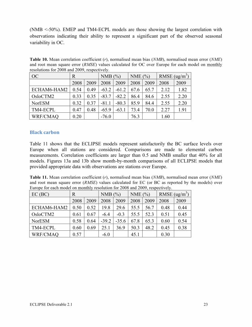
(NMB <-50%). EMEP and TM4-ECPL models are those showing the largest correlation with observations indicating their ability to represent a significant part of the observed seasonal variability in OC. Table 10. Mean correlation coefficient (r), normalised mean bias (NMB), normalised mean error (NME) and root mean square error (RMSE) values calculated for OC over Europe for each model on monthly resolutions for 2008 and 2009, respectively. OC R NMB (%) NME (%) RMSE (ug/m3)

2008 2009 2008 2009 2008 2009 2008 2009

ECHAM6-HAM2 0.54 0.49 -63.2 -61.2 67.6 65.7 2.12 1.82 OsloCTM2 0.33 0.35 -83.7 -82.2 86.4 84.6 2.55 2.20 NorESM 0.32 0.37 -81.1 -80.3 85.9 84.4 2.55 2.20 TM4-ECPL 0.47 0.48 -65.9 -63.1 73.4 70.0 2.27 1.91 WRF/CMAQ 0.20

-76.0

76.3

1.60

Black carbon Table 11 shows that the ECLIPSE models represent satisfactorily the BC surface levels over Europe when all stations are considered. Comparisons are made to elemental carbon measurements. Correlation coefficients are larger than 0.5 and NMB smaller that 40% for all models. Figures 13a and 13b show month-by-month comparisons of all ECLIPSE models that provided appropriate data with observations are stations over Europe. Table 11. Mean correlation coefficient (r), normalised mean bias (NMB), normalised mean error (NME) and root mean square error (RMSE) values calculated for EC (or BC as reported by the models) over Europe for each model on monthly resolution for 2008 and 2009, respectively. EC (BC) R NMB (%) NME (%) RMSE (ug/m3)

2008 2009 2008 2009 2008 2009 2008 2009

ECHAM6-HAM2 0.50 0.52 19.8 29.6 55.5 56.7 0.48 0.44 OsloCTM2 0.61 0.67 -6.4 -0.3 55.5 52.3 0.51 0.45 NorESM 0.58 0.64 -39.2 -35.6 67.8 65.3 0.60 0.54 TM4-ECPL 0.60 0.69 25.1 36.9 50.3 48.2 0.45 0.38 WRF/CMAQ 0.57

-6.0

45.1

0.30


Figure 13a: Comparison of monthly mean modelled BC (black carbon) with observations (black line with standard deviation). Model results are for the years 2009 (top) and 2008 (bottom) ECLIPSE models are indicated by colour : TM4-ECPL model (red), NOrESM (green), Oslo-CTM2 (yellow), ECHAM6-HAM2 (blue). All in µg m-3.

Figure 13b: Comparison of monthly mean modelled BC (black carbon) with observations (black line with standard deviation). Model results are for the years 2009 (top) and 2008 (bottom) ECLIPSE models are indicated by colour : TM4-ECPL model (red), NOrESM (green), Oslo-CTM2 (yellow), ECHAM6-HAM2 (blue). All in µg m-3.

Coarse and fine aerosols For PM10 (Table 12), EMEP global and WRF/CMAQ regional models have similar performances while for the PM2.5 (Table 13), EMEP global model performs much better than the regional model in terms of magnitudes. For both tracers the underestimations are lower than 50%. Figure 14 shows some comparison of global model results with observations for PM10 and Figure 15 for PM2.5. Table 12. Mean correlation coefficient (r), normalised mean bias (NMB), normalised mean error (NME) and root mean square error (RMSE) values calculated for PM10 over Europe for each model on monthly resolution for 2008 and 2009, respectively. PM10 R NMB (%) NME (%) RMSE (ug/m3)

2008 2009 2008 2009 2008 2009 2008 2009

EMEP 0.50 0.42 -22.0 -16.0 38.7 39.3 9.7 11.0 TM4-ECPL 0.36 0.29 72.9 78.4 59.4 57.7 12.3 13.3 WRF/CMAQ 0.27 -21.0 41.5 8.3


Figure 14. Comparison of global model results with observations of surface PM10 based on monthly mean values. Monthly mean observations using EBAS/EMEP databases are marked with symbols with standard deviation. Coloured lines show model results as explained in the figure’s legend.

Figure 15. Comparison of global model results with observations of surface PM2.5 based on monthly mean values. Monthly mean observations using EBAS/EMEP databases are marked with symbols with standard deviation. Coloured lines show model results as explained in the figure’s legend. Table 13. Mean correlation coefficient (r), normalised mean bias (NMB), normalised mean error (NME) and root mean square error (RMSE) values calculated for PM2.5 over Europe for each model on monthly resolution for 2008 and 2009, respectively. PM2.5 R NMB (%) NME (%) RMSE (ug/m3)

2008 2009 2008 2009 2008 2009 2008 2009

EMEP 0.27 0.34 -16.4 -12.1 45.4 42.1 15.2 10.7 TM4-ECPL 0.19 0.33 48.2 43.9 46.5 55.4 15.6 11.0 WRF/CMAQ 0.27 -50.2 55.6 9.2


Aerosol Optical Depth Table 15, 16, 17 show statistics for AOD@550nm, fine mode AOD and absorption AOD respectively as established against Aeronet sun photometer data. Table 15. Mean correlation coefficient (r), normalised mean bias (NMB), and root mean square error (RMSE) values calculated for AOD over World for each model on monthly resolution for 2008 and 2009, respectively. AOD@550nm R NMB (%) RMSE (ug/m3)

2008 2009 2008 2009 2008 2009

ECHAM 0.69 0.60 -46 -38 0.17 0.16 EMEP 0.82 0.81 +4 +4 0.13 0.13 NorESM 0.71 0.65 -15 -19 0.14 0.14 OsloCTM 0.71 - -27 - 0.14 - HadGEM 0.70 0.64 +15 +12 0.14 0.14 TM4-ECPL 0.67 0.75 +24 +3 0.25 0.14 Table 16. Mean correlation coefficient (r), normalised mean bias (NMB), and root mean square error (RMSE) values calculated for fine mode AODf over world for each model on monthly resolution for 2008 and 2009, respectively. AODf@550nm R NMB (%) RMSE (ug/m3)

2008 2009 2008 2009 2008 2009

ECHAM 0.76 0.56 -59 -49 0.14 0.12 EMEP 0.79 0.78 +7 +9 0.13 0.11 NorESM 0.52 0.41 -18 -22 0.13 0.12 TM4-ECPL 0.77 0.77 -40 -42 0.11 0.10 Table 17. Mean correlation coefficient (r), normalised mean bias (NMB), and root mean square error (RMSE) values calculated for absorption AOD (AAOD) over world for each model on monthly resolution for 2008 and 2009, respectively. AAOD@550nm R NMB (%) RMSE (ug/m3)

2008 2009 2008 2009 2008 2009

ECHAM 0.75 0.73 -65 -65 0.018 0.018 OsloCTM 0.68 - -54 - 0.017 - NorESM 0.65 0.66 -57 -60 0.019 0.019 HadGEM 0.65 0.58 -94 -93 0.025 0.024


ECLIPSE Publications Daskalakis N., Myriokefalitakis S., Kanakidou M: Global Ozone and Organic Aerosol sensitivity to biomass burning emissions, EGU 2013, Vienna April 2013 (poster)

Im U., S. Christodoulaki, K. Violaki, P. Zarbas, M. Kocak, N. Daskalakis, N. Mihalopoulos and M. Kanakidou, Atmospheric deposition of nitrogen and sulfur over Europe with focus on the Mediterranean and the Black Sea, Atmospheric Environment, 81, 660-670, http://dx.doi.org/10.1016/ j.atmosenv.2013.09.048, 2013.

Im U., Daskalakis N., Markakis K., Vrekoussis M., Hjorth J., Myriokefalitakis S., Gerasopoulos E., Kouvarakis G., Richter A., Burrows J., Pozzoli L., Unal A., Kindap T., Kanakidou M., Simulated Air Quality and Pollutant Budgets over Europe in 2008, Science of Total Environment, 10.1016/j.scitotenv.2013.09.090, 470–471, 270–281, 2014.

Tsigaridis K., Daskalakis N., Kanakidou M et al., The AeroCom evaluation and intercomparison of organic aerosol in global models, The AeroCom evaluation and intercomparison of organic aerosol in global models. Atmos. Chem. Phys. 2014, 14 (19), 10845-10895.

Myriokefalitakis S., Daskalakis N., et al., Pollution over the Eastern Mediterranean: The Importance of Long – Range Transport in preparation for ACPD, 2014


APPENDIX: List of stations over Europe used for the model evaluation.

Table S1. Surface stations monitoring gaseous pollutants over Europe, used for the model evaluation Station Code Station Name Country Lat Lon Alt AT0002R Illmitz Austria 47.77 16.46 117 AT0005R Vorhegg Austria 46.68 12.97 1020 AT0030R Pillersdorf bei Retz Austria 48.72 15.94 315 AT0032R Sulzberg Austria 47.53 9.93 1020 AT0034G Sonnblick Austria 47.05 12.96 3106 AT0037R Zillertaler Alpen Austria 47.14 11.87 1970 AT0038R Gerlitzen Austria 46.69 13.92 1895 AT0040R Masenberg Austria 47.35 15.88 1170 AT0041R Haunsberg Austria 47.97 13.02 730 AT0042R Heidenreichstein Austria 48.88 15.05 581 AT0043R Forsthof Austria 48.11 15.92 581 AT0044R Graz Platte Austria 47.11 15.42 651 AT0045R Dunkelsteinerwald Austria 48.37 15.55 320 AT0046R Gänserndorf Austria 48.33 16.73 161 AT0047R Stixneusiedl Austria 48.05 16.68 240 AT0048R Zoebelboden Austria 47.84 14.44 899 AT0049R Grebenzen Austria 47.04 14.33 1648 BG0053R Rojen peak Bulgaria 41.70 24.74 1750 CH0001G Jungfraujoch Switzerland 46.55 7.99 3578 CH0002R Payerne Switzerland 46.81 6.85 489 CH0003R Tänikon Switzerland 47.48 8.91 539 CH0004R Chaumont Switzerland 47.05 6.98 1137 CH0005R Rigi Switzerland 47.07 8.46 1031 CZ0001R Svratouch Czech Republic 49.73 16.05 737 CZ0003R Kosetice Czech Republic 49.58 15.08 534 CY0002R Ayia Marina Cyprus 35.04 33.06 532 DE0001R Westerland Germany 54.93 8.31 12 DE0002R Waldhof Germany 52.80 10.76 74 DE0003R Schauinsland Germany 47.92 7.91 1205 DE0007R Neuglobsow Germany 53.17 13.03 62 DE0008R Schmücke Germany 50.65 10.77 937 DE0009R Zingst Germany 54.43 12.73 1 DE0043G Hohenpeissenberg Germany 47.80 11.02 985 DE0044R Melpitz Germany 51.53 12.93 86 ES0007R Víznar Spain 37.23 -3.53 1265 ES0008R Niembro Spain 43.44 -4.85 134


ES0009R Campisabalos Spain 41.28 -3.14 1360 ES0010R Cabo de Creus Spain 42.32 3.32 23 ES0011R Barcarrola Spain 38.48 -6.92 393 ES0012R Zarra Spain 38.09 -1.10 885 ES0013R Penausende Spain 41.28 -5.87 985 ES0014R Els Torms Spain 41.40 0.72 470 ES0016R O Saviñao Spain 43.23 -7.70 506 ES1778R Montseny Spain 41.77 2.35 700 FR0009R Revin France 49.90 4.63 390 FR0010R Morvan France 47.27 4.08 620 FR0012R Iraty France 43.03 -1.08 1300 FR0013R Peyrusse Vieille France 43.62 0.18 200 FR0014R Montandon France 47.30 6.83 836 FR0015R La Tardière France 49.65 -0.75 133 FR0016R Le Casset France 45.00 6.47 1750 FR0017R Montfranc France 45.80 2.07 810 FR0018R La Coulonche France 48.63 -0.45 309 FR0030R Puy de Dôme France 45.77 2.95 1465 HU0002R K-puszta Hungary 46.97 19.58 125 IT0001R Montelibretti Italy 42.10 12.63 48 IT0004R Ispra Italy 45.80 8.63 209 MK0007R Lazaropole Macedonia 41.32 20.25 1332 MD0013R Leova II Moldova 46.49 28.28 166 PL0005R Diabla Gora Poland 54.15 22.07 157 PT0004R Monte Velho Portugal 38.08 -8.80 43 RS0005R Kamenicki vis Serbia 43.40 21.95 813 SI0008R Iskrba Slovenia 45.57 14.87 520 SI0032R Krvavec Slovenia 46.30 14.54 1740 SK0006R Starina Slovakia 49.05 22.27 345


Table S2. Surface stations monitoring particulate pollutants over Europe, used for the model evaluation StationCode StationName Country Lat Lon Alt AT0002R Illmitz Austria 47.77 16.46 117 AT0005R Vorhegg Austria 46.68 12.97 1020 AT0030R Pillersdorf bei Retz Austria 48.72 15.94 315 AT0032R Sulzberg Austria 47.53 9.93 1020 AT0034G Sonnblick Austria 47.05 12.96 3106 AT0037R Zillertaler Alpen Austria 47.14 11.87 1970 AT0038R Gerlitzen Austria 46.69 13.92 1895 AT0040R Masenberg Austria 47.35 15.88 1170 AT0041R Haunsberg Austria 47.97 13.02 730 AT0042R Heidenreichstein Austria 48.88 15.05 581 AT0043R Forsthof Austria 48.11 15.92 581 AT0044R Graz Platte Austria 47.11 15.42 651 AT0045R Dunkelsteinerwald Austria 48.37 15.55 320 AT0046R Gänserndorf Austria 48.33 16.73 161 AT0047R Stixneusiedl Austria 48.05 16.68 240 AT0048R Zoebelboden Austria 47.84 14.44 899 AT0049R Grebenzen Austria 47.04 14.33 1648 BG0053R Rojen peak Bulgaria 41.70 24.74 1750 CH0001G Jungfraujoch Switzerland 46.55 7.99 3578 CH0002R Payerne Switzerland 46.81 6.85 489 CH0003R Tänikon Switzerland 47.48 8.91 539 CH0004R Chaumont Switzerland 47.05 6.98 1137 CH0005R Rigi Switzerland 47.07 8.46 1031 CZ0001R Svratouch Czech Republic 49.73 16.05 737 CZ0003R Kosetice Czech Republic 49.58 15.08 534 CY0002R Ayia Marina Cyprus 35.04 33.06 532 DE0001R Westerland Germany 54.93 8.31 12 DE0002R Waldhof Germany 52.80 10.76 74 DE0003R Schauinsland Germany 47.92 7.91 1205 DE0007R Neuglobsow Germany 53.17 13.03 62 DE0008R Schmücke Germany 50.65 10.77 937 DE0009R Zingst Germany 54.43 12.73 1 DE0043G Hohenpeissenberg Germany 47.80 11.02 985 DE0044R Melpitz Germany 51.53 12.93 86 ES0007R Víznar Spain 37.23 -3.53 1265 ES0008R Niembro Spain 43.44 -4.85 134 ES0009R Campisabalos Spain 41.28 -3.14 1360 ES0010R Cabo de Creus Spain 42.32 3.32 23


ES0011R Barcarrola Spain 38.48 -6.92 393 ES0012R Zarra Spain 38.09 -1.10 885

Table S2. continued

StationCode StationName Country Lat Lon Alt ES0013R Penausende Spain 41.28 -5.87 985 ES0014R Els Torms Spain 41.40 0.72 470 ES0016R O Saviñao Spain 43.23 -7.70 506 ES1778R Montseny Spain 41.77 2.35 700 FR0009R Revin France 49.90 4.63 390 FR0010R Morvan France 47.27 4.08 620 FR0012R Iraty France 43.03 -1.08 1300 FR0013R Peyrusse Vieille France 43.62 0.18 200 FR0014R Montandon France 47.30 6.83 836 FR0015R La Tardière France 49.65 -0.75 133 FR0016R Le Casset France 45.00 6.47 1750 FR0017R Montfranc France 45.80 2.07 810 FR0018R La Coulonche France 48.63 -0.45 309 FR0030R Puy de Dôme France 45.77 2.95 1465 HU0002R K-puszta Hungary 46.97 19.58 125 IT0001R Montelibretti Italy 42.10 12.63 48 IT0004R Ispra Italy 45.80 8.63 209 MD0013R Leova II Moldova 46.49 28.28 166 PL0005R Diabla Gora Poland 54.15 22.07 157 PT0004R Monte Velho Portugal 38.08 -8.80 43 SI0008R Iskrba Slovenia 45.57 14.87 520 SK0004R Stará Lesná Slovakia 49.15 20.28 808 SK0006R Starina Slovakia 49.05 22.27 345 SK0007R Topolniky Slovakia 47.96 17.86 113


Table S3. Surface stations in Istanbul and Athens and Finokalia remote monitoring station, used for model evaluation. Station Lat (o) Lon (o) Alt (m) ISTANBUL Alibeykoy 41.07 28.95 60 Besiktas 41.05 29.01 94 Esenler 41.04 28.89 59 Kadikoy 40.99 29.03 6 Sariyer 41.70 29.05 103 Uskudar 41.02 29.03 70 Yenibosna 40.59 28.49 23 ESC (Bogazici University) 41.09 29.05 80 Kandilli 41.06 29.06 125 ATHENS Ag. Paraskevi 38.00 23.82 290 Aristotelous 37.99 23.73 95 Athinas 37.98 23.73 100 Lykovrysi 38.07 23.78 210 Marousi 38.03 23.79 145 Patision 38.00 23.73 105 Thrakomakedones 38.14 23.76 550 Penteli 37.58 23.43 107 Geoponiki 37.98 23.71 50 Liosia 38.08 23.70 165 Elefsina 38.05 23.58 20 Smyrni 37.93 23.72 50 Peristeri 38.02 23.70 80 Pireas 37.94 23.65 20 FINOKALIA 35.20 25.40 250


Table S4. AERONET stations over Europe used for model evaluation and the statistics in Table 14. Station Country Lat Lon Height Blida Algeria 36.508 2.881 230 Kanzelhohe_Obs Austria 46.678 13.907 1526 Carpentras France 44.083 5.058 100 Dunkerque France 51.035 2.368 0 Fontainebleau France 48.407 2.68 85 Lille France 50.612 3.412 60 Palaiseau France 48.7 2.208 156 Paris France 48.867 2.333 48.867 Hamburg Germany 53.568 9.973 105 Helgoland Germany 54.178 7.887 33 IFT-Leipzig Germany 51.352 12.435 125 Karlsruhe Germany 49.093 8.428 140 Mainz Germany 49.999 8.3 150 Athens NOA Greece 37.988 23.775 130 FORTH Crete Greece 35.333 25.282 20 Thessaloniki Greece 40.63 22.96 60 Xanthi Greece 41.147 24.919 54 Eliat Israil 29.503 34.917 15 Nes Ziona Israel 31.922 34.789 40 SEDE BOKER Israel 30.855 34.782 480 IMAA Potenza Italy 40.6 15.72 820 Ispra Italy 45.803 8.627 235 Lecce University Italy 40.335 18.111 30 Tremiti Italy 42.118 15.49 4 Moldova Moldova 47 28.816 205 Baneasa Romania 44.511 26.078 127 Bucharest Inoe Romania 44.348 26.03 93 Autilla Spain 41.997 -4.603 873 Caceres Spain 39.479 -6.343 397 Granada Spain 37.164 -3.605 680 Davos Switzerland 46.813 9.844 1596 Laegeren Switzerland 47.48 8.351 735 IMS METU Turkey 36.565 34.255 3

deliverable 2.1 v2 1 8 14 - eclipse.nilu.noeclipse.nilu.no/portals/83/project...

Documents