deliverable d3.1 initial report on ai-driven techniques

871780 — MonB5G — ICT-20-2019-2020

Deliverable D3.1 Initial Report on AI-Driven Techniques for the

MonB5G AE/MS

Document Summary Information

Grant Agreement No 871780 Acronym MonB5G

Full Title Distributed Management of Network Slices in beyond 5G

Start Date 01/11/2019 Duration 36 months

Project URL https://www.monb5g.eu/

Deliverable D3.1 – Initial Report on AI-Driven Techniques for the MonB5G AE/MS

Work Package WP3

Contractual due date M17 Actual submission date 31.03.2021

Nature Report Dissemination Level Public

Lead Beneficiary NEC

Responsible Author Zhao Xu (NEC)

Contributions from Christos Verikoukis (CTTC), Hatim Chergui (CTTC), Luis Blanco (CTTC), Luis Sanabria-Russo (CTTC), David Pubill (CTTC), Jordi Serra (CTTC), Sarang Kahvazadeh (CTTC), George Tsolis (CTXS), Christos Tselios (CTXS), Luis A. Garrido Platero (IQU), Anne-Marie Bosneag (LMI), Zhao Xu (NEC), Amina Boubendir (ORA-FR), José Jurandir Alves Esteves (ORA-FR), Sławomir Kukliński (ORA-PL)

https://upload.wikimedia.org/wikipedia/commons/b/b7/Flag_of_Europe.svg

https://www.monb5g.eu/

871780 — MonB5G — ICT-20-2019-2020

Deliverable D3.1 – Initial Report on AI-Driven Techniques for the MonB5G AE/MS [Public]

©MonB5G, 2019 Page | 2

Revision history

Version Issue Date Complete(%) Changes Contributor(s)

V0.1 16/11/2020 1 Initial Deliverable Structure and ToC

Anne-Marie Bosneag, Amina Boubendir, Hatim Chergui, Sławomir Kukliński, George Tsolis, Zhao Xu

V0.2 07/12/2020 10 Scope and planed contributions of each (sub)section

All partners

V0.3 22/02/2021 70 Initial draft All partners

V0.4 10/03/2021 80 Analyse the potential gaps in the sections and give comments to improve

Anne-Marie Bosneag, Amina Boubendir, Hatim Chergui, Sławomir Kukliński, George Tsolis, Zhao Xu

V1 20/03/2021 90 Complete version All partners

V2 30/03/2021 100 Further improve the first complete version by polishing the descriptions, bridging the minor gaps, integrating recent SOTA works and specifications etc.

All partners

Disclaimer

The content of the publication herein is the sole responsibility of the publishers and it does not necessarily represent the views expressed by the European Commission or its services.

While the information contained in the documents is believed to be accurate, the authors(s) or any other participant in the MonB5G consortium make no warranty of any kind with regard to this material including, but not limited to the implied warranties of merchantability and f itness for a particular purpose.

Neither the MonB5G Consortium nor any of its members, their officers, employees or agents shall be responsible or liable in negligence or otherwise howsoever in respect of any inaccuracy or omission herein.

Without derogating from the generality of the foregoing neither the MonB5G Consortium nor any of its members, their officers, employees or agents shall be liable for any direct or indirect or consequential loss or damage caused by or arising from any information advice or inaccuracy or omission herein.

Copyright message

© MonB5G Consortium, 2019-2022. This deliverable contains original unpublished work except where clearly indicated otherwise. Acknowledgement of previously published material and of the work of others has b een made through appropriate citation, quotation or both. Reproduction is authorised provided the source is acknowledged.

871780 — MonB5G — ICT-20-2019-2020



TABLE OF CONTENTS

List of Figures ............................................................................................................................................... 5

List of Tables ................................................................................................................................................ 7

List of Acronyms ........................................................................................................................................... 8

1 Executive summary ...............................................................................................................................11

2 Introduction .........................................................................................................................................14

2.1 Scope ............................................................................................................................................14

2.2 Target Audience ...........................................................................................................................14

2.3 Structure ......................................................................................................................................14

3 Monitoring System for 5G Networks .....................................................................................................16

3.1 Overview of Monitoring Systems ..................................................................................................16

3.2 New Requirements Driven by 5G Networks and Beyond ...............................................................18

3.3 Data Availability and Collection ....................................................................................................19

3.4 Domain-Specific MS ......................................................................................................................21

3.4.1 MS for RAN ...............................................................................................................................21

3.4.2 MS for Edge ..............................................................................................................................21

3.4.3 MS for Cloud .............................................................................................................................23

4 Data Analytics Functions in 5G Networks ..............................................................................................25

4.1 Overview ......................................................................................................................................25

4.1.1 3GPP NWDAF ............................................................................................................................25

4.1.2 ETSI zsm ....................................................................................................................................30

4.2 ML/AI Techniques for Data Analytics ............................................................................................31

4.2.1 Time Series Forecasting .............................................................................................................31

4.2.2 Classification and Anomaly Detection .......................................................................................33

4.2.3 Graph Representation Learning .................................................................................................33

4.2.4 Federated Learning ...................................................................................................................34

4.2.5 Reinforcement Learning ............................................................................................................35

4.3 Solutions on Data Analytics Using ML/AI Techniques ....................................................................36

4.3.1 DRL Approach using Graph Convolutional Networks ..................................................................36

4.3.2 DeepViNE: Virtual Network Embedding with Deep Reinforcement Learning ..............................37

4.3.3 DRL-based Dynamic Resource Allocation (DRA) Scheme ............................................................37

871780 — MonB5G — ICT-20-2019-2020



4.3.4 Adaptive DRL approach for Service Function Chains (SFCs) Deployment ....................................38

4.3.5 Dynamic Policy Network based RL for VNE ................................................................................39

4.3.6 DRL in Multi-Domain Non-Cooperative VNF-FG Embedding .......................................................39

5 MonB5G Monitoring System .................................................................................................................42

5.1 Selection of Slice KPIs and Monitored Parameters ........................................................................42

5.2 Architecture of MonB5G MS .........................................................................................................45

5.3 Domain-specific MS ......................................................................................................................48

5.3.1 MS in the RAN domain ..............................................................................................................49

5.3.2 MS in the edge/cloud domain ...................................................................................................50

5.4 Cooperation of MS with AE and DE ...............................................................................................52

6 MonB5G AE Vision ................................................................................................................................54

6.1 AE Structure and Interfaces ..........................................................................................................54

6.1.1 KPI Prediction ...........................................................................................................................54

6.1.2 Fault Detection .........................................................................................................................54

6.1.3 AE Interfaces with MS and DE ...................................................................................................55

6.2 AE Cross-Domain Operation ..........................................................................................................56

7 MonB5G Analytics Engine for Slice-Level KPI Prediction ........................................................................59

7.1 Local KPI Prediction ......................................................................................................................59

7.2 Cross-Domain KPI Prediction .........................................................................................................62

7.3 Network Aware KPI Prediction ......................................................................................................69

7.3.1 Context-Aware Demand Predictors ...........................................................................................69

7.3.2 RAN-MEC split ConvNet architectures for network-aware KPI prediction ..................................74

8 MonB5G Analytics Engine for Network Fault Management ...................................................................78

8.1 Fault management problem description .......................................................................................78

8.2 Local Analytics Engine for Fault Management ...............................................................................78

8.3 Cross-Domain Analytics Engine for Fault Management .................................................................79

8.4 Interactions with Other MonB5G Management/Orchestration Components .................................81

9 Conclusions ..........................................................................................................................................82

871780 — MonB5G — ICT-20-2019-2020



List of Figures Figure 1 Monitoring Agents from the Perspective of Functions and Cloud Infrastructure ........................................................ 24

Figure 2 NWDAF Interactions with NFs ................................................................................................................................... 26

Figure 3 Distributed Architecture of NWDAF in R16 and R17 ................................................................................................ 29

Figure 4 MDAS at Different Levels .......................................................................................................................................... 29

Figure 5 Functional View of a Closed Loop and its Functions within the ZSM Framework [16] ............................................. 30

Figure 6 Architecture of the MonB5G Monitoring System ....................................................................................................... 45

Figure 7 MS Request and Metrics Retrieval from Monitored Element ..................................................................................... 47

Figure 8 Mapping Sampling Loop Orchestration to Implementation Tools .............................................................................. 48

Figure 9 MonB5G MS in the RAN Domain .............................................................................................................................. 50

Figure 10 MonB5G MS in the Edge/Cloud Domain ................................................................................................................. 51

Figure 11 MS Interfaces ............................................................................................................................................................ 52

Figure 12 Local AE Functions ................................................................................................................................................... 54

Figure 13 AE Interfaces ............................................................................................................................................................. 55

Figure 14 Example Application of Decentralized Model Training. a) Data at Each Node; b) and c) Two Different Network

Topologies; d) Difference in the Convergence Speed ....................................................................................................... 57

Figure 15 Cross-Domain AE Cooperation via Federated Learning ........................................................................................... 58

Figure 16 Cross-Domain AE Cooperation via Distributed NN ................................................................................................. 58

Figure 17 Vanilla LSTM Neural Network. Left: Lag Signals (Inputs). Right: Predicted Signal of the Next Time Instance

(Outputs) ............................................................................................................................................................................ 60

Figure 18 Training Loss vs Epochs for Vanilla LSTMs with Different Memory Sizes ............................................................ 60

Figure 19 Enhanced LSTM Neural Network with Traffic and Meta Information as Inputs to Predict the Traffic of the Next

Time Instance. .................................................................................................................................................................... 61

Figure 20 Training Loss vs Epochs for Enhanced LSTMS with Meta Data, Tested with Different Memory Sizes.................. 61

Figure 21 Traffic Intensity (Prediction and Ground Truth) for 6 Different BSs ........................................................................ 62

Figure 22 Network Architecture with Decentralized MS/AE at the Edge and Cloud Domains ................................................ 63

Figure 23 DL PRBs Distributions, with α = [0, 0, 0], β= [15, 10, 10] PRBs and γ = [0.01, 0.01, 0.01]. ................................... 66

Figure 24 CPU Load Distributions, with α = [0, 0, 0], β = [4, 7, 10], and γ = [0.01, 0.01, 0.01]. ............................................. 67

Figure 25 CPU Load Average Violation Rates with α = [0, 0, 0], β= [4, 7, 10], and γ = [0.01, 0.01, 0.01]. ............................. 67

Figure 26 Convergence of SFL vs. CCL Scheme for CDF SLA with α = [0, 0, 0], β= [15, 10, 10] PRBs ............................... 68

871780 — MonB5G — ICT-20-2019-2020



Figure 27 DDNN Architecture for Network-Aware KPI Prediction: the Local Part of the NN in the RAN (near the BSs) and

the Remote Part in the MEC .............................................................................................................................................. 75

Figure 28 Distributed CNN for Slice State Recognition ............................................................................................................ 80

871780 — MonB5G — ICT-20-2019-2020



List of Tables Table 1 Deliverable Structure and Mapping with Project Tasks ............................................................................................... 14

Table 2 NF Services Provided by NWDAF ............................................................................................................................... 28

Table 3 Analytics Information Provided by NWDAF ............................................................................................................... 28

Table 4 Mapping between the High-Level Project KPIs and the Selected Slice-Level KPIs .................................................... 42

Table 5 Slice-Level KPIs Description and Measurement .......................................................................................................... 44

Table 6 MS Interfaces and the Associated Roles ....................................................................................................................... 53

Table 7 AE Interfaces and the Associated Roles ....................................................................................................................... 56

Table 8 Features of the Simulated Datasets ............................................................................................................................... 63

Table 9 Communication Overhead Comparison ........................................................................................................................ 68

871780 — MonB5G — ICT-20-2019-2020



List of Acronyms

Acronym Description

3GPP Third Generation Partnership Project

AE Analytic Engine

AE-F Analytic Engine Function

AE-S Analytic Engine Sublayer

AI Artificial Intelligence

CLA Closed-loop Automation

CNF Cloud Native function

DE Decision Engine

DE-F Decision Engine Function

DE-S Decision Engine Sublayer

EEM Embedded Element Manager

eMBB Enhanced Mobile Broadband

eTOM Enhanced Telecom Operations Map

ETSI European Telecommunications Standards Institute

ECA Event Condition Action

ENI Experiential Networked Intelligence

FCAPS Fault, Configuration, Accounting, Performance, Security

ISM In-Slice Management

ITU International Telecommunication Union

KPI Key Performance Indicator

LCM Lifecycle Management

ML Machine Learning

MANO Management and Orchestration

MaaS Management as a Service

MAN-F Management Function

mMTC Massive Machine Type Communications

MEO MEC Orchestrator

871780 — MonB5G — ICT-20-2019-2020



MNO Mobile Network Operator

MLaaS MonB5G Layer as a Service

MS Monitoring System

MS-F Monitoring System Function

MS-S Monitoring System Sublayer

MEC Multi-access Edge Computing

NFVO Network Function Virtualization Orchestrator

NSD Network Service Descriptor

NSO Network Service Orchestrator

NSP Network Service Provider

NSI Network Slice Instance

NSMF Network Slice Management Function

NSSMF Network Slice Subnetwork Management Function

NST Network Slice Template

NSSI Network sub-Slice Instance

NGMN Next Generation Mobile Networks

NFVI NFV Infrastructure

OAI Open Air Interface

ONAP Open Network Automation Platform

OSM Open-Source MANO

OSS Operation System Support

PaaS Platform as a Service

PoC Proof of Concept

QoE Quality of Experience

QoS Quality of Service

RAN Radio Access Network

SON Self-Organizing Network

SLA Service Level Agreement

SFL Slice Functional Layer

SML Slice Management Layer

871780 — MonB5G — ICT-20-2019-2020


©MonB5G, 2019 Page | 10

SM Slice Manager

uRLLC Ultra-Reliable Low-Latency Communication

VIM Virtual Infrastructure Manager

VNF Virtual network Function

VNFM Virtual network Function Manager

ZSM Zero-touch network and Service Management

871780 — MonB5G — ICT-20-2019-2020


©MonB5G, 2019 Page | 11

1 Executive summary

The work package 3 of the MonB5G project aims to develop distributed AI-based analytics engine (AE) and monitoring system (MS) that are designed and implemented as the essential management and orchestration components to support massive network slicing for 5G networks and beyond. This deliverable is an initial report to present the current achievements of the innovative MS and AE, and the final results with enhanced features, extra functions and detailed verification will be reported in the Deliverable 3.2.

With new pervasive mobile services of a variety of vertical industries, the centralized network management system faces considerable challenges to address massive numbers of coexisting slices, which have different performance requirements, functionality, and timespans. To enable a highly intelligent, scalable and energy efficient slice management, the MS and AE of the system need to shift their operations towards a distributed, data-driven framework with few human interventions, and be able to efficiently and proactively cope with novel vulnerabilities. MonB5G meets these new requirements and challenges on AE and MS for 5G networks and beyond, and develops the distributed AI-based network management entities, which are locally deployed in different technical domains but interoperate together to automatically manage the slices with focuses on their service quality, energy effectiveness, as well as communication resource optimization.

MonB5G implements a scalable MS architecture that is based on autonomic network management specifications and cloud-native design. MonB5G MS can be conceived as a cross-domain virtual layer hosted by a NFV IFA 029-compliant PaaS (i.e., Container Infrastructure System (CIS)). The deployment of the MS follows the concept of Slice Management Layer (SML) as a Service proposed in the MonB5G architecture in Deliverable 2.1. The distributed MonB5G MS collects the current operation status at multiple levels of the management hierarchy (node, slice, domain, and inter-domain) in a programmable manner. After triggered and configured by AEs, the programmable MS entities connects the corresponding infrastructure and network functions (VNFs and PNFs) to gather the requested telemetries with the specific granularity defined by the AEs. There are mainly three types of APIs associated with each MS entity, including Control API, Data Collection API, and Data Processing API, which connect with a MS-bus to handle real-time data feeds for a unified, high-throughput and low-latency communication. The MonB5G monitoring system achieves the following advantages:

The distributed MS agents are designed to manage the tightest metrics sampling loops in its respective technological domain, such that the need for data transfer is largely reduced, and thus communication overhead introduced by the monitoring system itself is minimized.

Additionally, an extra MAPE-based embedded element manager (EEM) is deployed at VNF level to support fine granularity (1s) of telemetry collection. It also permits development of aggregators for specific (e.g., slice-level) AE and DE.

More importantly the configurations of MS entities distributed at different technical domains are automatically defined and triggered by the AE/DE components with AI-assisted policy-driven mechanisms, which take a crucial step towards highly automated slice-level monitoring system.

The MonB5G analytics engine aims to analyse the status of massive numbers of coexisting slices with inter -domain, cross-domain and network-aware KPI inspection. We have developed a variety of AE functions to fulfill diverse predictions and fault detection at the different levels of the orchestration hierarchy, including context-aware traffic prediction, feature extraction of native data, resource estimation with low SLA

871780 — MonB5G — ICT-20-2019-2020


©MonB5G, 2019 Page | 12

violation, slice state recognition etc. In particular, the current version of the AE entities has implemented some essential features, such as:

Enhanced traffic prediction: traffic load forecasting is essential for many downstream tasks, such as resource allocation and admission control. We develop an innovative AE to predict traffic load in the RAN domain with augmented information. The input data not only includes the historical traffic measurements, but also augment with additional information, such as base station (BS) data, day of the week and time of the day. A mechanism of training centrally and predicting locally is explored to improve scalability and maintain high prediction accuracy in the meanwhile.

Network aware KPI prediction: in order to reduce the gap between demand prediction and resource orchestration, it is necessary to make the predictive AEs aware of the context information, i.e., exploiting knowledge from the resource orchestration problem domain in the demand-forecasting task. This AE entity integrates additional regularizations to model penalty for the settings of over - and under-allocation resources, as well as for resource re-allocation. By ensuring that the proper amount of resource is made available to a network slice when needed, it significantly reduces the probability of the SLA violations and thus guarantees the users’ perceived QoS.

Federated Resource estimation with low SLA violation: this AE function introduces a set of well-designed statistical constraints towards distributed network management with enhanced federated learning. The novel function will facilitate network slicing decentralized resource allocation while guaranteeing very low service-level agreement (SLA) violations.

Slice state recognition: in order to manage a massive number of slices, it is critical to know status of any slice running on a network infrastructure. This AE function aims to classify the state of a slice for every time step conditioned on a set of measurements of the monitored slice. Importantly, we develop a distributed deep neural network method that is based on the estimated certainty of the status estimation. With a predefined certainty threshold, the AE function will predict locally to reduce communication overhead and potential latency, or offload the compressed local outputs to the higher level of the management hierarchy to estimate with more information for a more confident prediction.

In the developed MonB5G AE entities, the novel distributed machine learning (ML) and representation learning algorithms are implemented and tailored to fulfil the requirements of 5G networks and beyond, such that the traditionally centralized AE can be decomposed into inter-connected entities deployed in a distribution manner in the RAN, edge and cloud domains. This allows highly intelligent, accurate, and scalable reactions to non-stationary network conditions, new traffic patterns and evolving slice characteristics. The distribution of the MonB5G AE includes multiple levels, such as learning concise representations of local data to reduce the amount of the information exchanged for management purposes, as well as boosting slice -level KPI prediction and the corresponding AI models with different native data. These properties and advantages significantly reduce communication overhead and processing operations needed to cope with the unprecedented amount of big data generated by 5G networks, in addition improve prediction and learning accuracy with considerably decreased reaction time for sensitive slice management under stringent time constraints.

So far, the MonB5G MS and AE have introduced a distributed AI-driven management mechanism to meet a set of new challenges in massive network slicing, including scalability, automation, and efficiency of heterogeneous resources (e.g., communication, computation, storage and energy). The developed

871780 — MonB5G — ICT-20-2019-2020


©MonB5G, 2019 Page | 13

framework reuses standards-based MANO and MEC frameworks and extends them with locally embedded intelligence capabilities. The work package 3 releases a comprehensive solution for autonomic slice-level network monitoring and analysis, which allows for accurately predicting network KPIs, proactively identifying potential vulnerabilities, faults and misconfigurations, as well as providing analysis results to the decision engine developed in WP4 for predictive resource management and optimization.

871780 — MonB5G — ICT-20-2019-2020


©MonB5G, 2019 Page | 14

2 Introduction

2.1 Scope

This is a public deliverable of MonB5G project’s Work Package 3 (WP3) describing the current status of progress and achievements, as well as the developed innovative management entities that enable intelligent and scalable monitoring and analysis in a distributed AI-driven manner. This deliverable reviews state-of-the-art monitoring systems and analytics tools, discusses new requirements and relevant specifications needed for zero-touch management of massive coexisting network slices, before conclusion introduces the initial version of the proposed cloud native MS and AE entities that are empowered by new advances in distributed AI technologies to improve intelligence and scalability of network management for fully leveraging diverse resource and promoting slice-level service quality.

2.2 Target Audience

The target audience of this deliverable are stakeholders related to zero-touch management and orchestration of 5G technologies and infrastructure, especially the ones with focuses on slice-level monitoring and analysis of miscellaneous network domains. The deliverable describes the distributed AI-driven management entities that are used to build and enhance intelligence, scalability and cost-effectiveness of 5G networks.

2.3 Structure

The main technical sections of the deliverable are organized as the following table. In the table, we also map the committed tasks of the grant agreement (GA) with the outputs reported in this delive rable in order to further clarify and position the innovative contributions under the framework of the MonB5G project.

Table 1 Deliverable Structure and Mapping with Project Tasks

Section Description Task(s) Starting Month

3

Investigates state-of-the-art monitoring systems, new requirements and challenges introduced by management of a massive number of coexisting network slices, as well as the potential opportunities for the stakeholders.

T3.1 M4

4

Explores functionalities and techniques of leading analytics tools implemented in the current network management platforms, leading-edge AI algorithms utilized in diverse network management tasks, and a variety of specifications instructing intelligent monitoring and analysis of network functions/slices.

T3.2 & T3.3 M7

871780 — MonB5G — ICT-20-2019-2020


©MonB5G, 2019 Page | 15

5

Selects slice-level KPIs and network measurements that need to be monitored with focuses on the MonB5G innovations, illustrates distributed MS entities deployed in RAN, edge and cloud domains, as well as the first version of the MS framework that follows a cloud-native approach, where different sampling loops can be configured and created for specific management goals.

T3.1 M4

6

Introduces insight and vision of MonB5G about analytics engine. The AE functions, structure and interfaces between AE and DE/MS are explained to give a big picture of the design of MonB5G AE. The mechanisms and technologies utilized to fulfill AE cross-domain operations are also reported.

T3.2 & T3.3 M7

7

Presents slice-level KPI prediction, including local KPI prediction in RAN, edge and cloud domains, cross-domain KPI prediction that involves status and measurements of multiple domains, and network aware KPI prediction with distributed AI techniques.

T3.2 M7

8

Introduces AE for network fault management. It starts with diverse scenarios where fault management is essential, then proposes fault detection mechanisms with local data, after that, the distributed and cross-domain fault management is discussed to correctly identify complicated faults with comprehensive analysis. Finally, the interoperation between fault management engine and other entities of the MonB5G platform is presented.

T3.3 M7

871780 — MonB5G — ICT-20-2019-2020


©MonB5G, 2019 Page | 16

3 Monitoring System for 5G Networks

3.1 Overview of Monitoring Systems

Observability, consisting of monitoring, logging and tracing, are crucial requirements of any service deployment [1]. In general, observability involves gathering data about the operation of services, typically referred to as “telemetry”. Modern service platforms, infrastructures and frameworks have observability systems in place that gather four types of telemetries:

Metrics: Time-series data that typically measure the four “golden signals” of monitoring: latency, traffic, errors, and saturation. Based on the collected metrics, analysis can be done to provide aggregations, slicing & dicing, statistical analysis, outlier detection and alerting capabilities. DevOps depends on these metrics to understand the performance, throughput, reliability and scale of the services. They also monitor Service Level Indicators (SLIs) to detect any deviations from Service Level Objectives (SLOs), ideally before they lead to SLA (Service Level Agreement) violations.

Events/Alerts: network operators and service providers often pre-define a set of threshold or rules w.r.t. the metrics at different technical domains and infrastructure, whenever a threshold/rule is crossed, then an event or alert will be triggered, a notification is generated and transferred to the corresponding functional components to resolve possible issues.

Logs: As traffic flows into a service, a full record of each request will be generated, including source and destination metadata. This information enables DevOps to audit service behaviour down to the individual service instance level. Analysis is typically done via search UIs that filter logs based on queries and patterns, indispensable for troubleshooting and root cause analysis of operational issues.

Traces: Timestamped records about the handling of the requests, or “calls”, by service instances. As a result of the decomposition of network services into many VNFs and of monoliths into numerous micro -services, and the creation of service chains/meshes that route calls between them, modern service infrastructures offer distributed tracing capabilities. They generate trace spans for each service, providing DevOps with detailed visibility of call flows and service dependencies within a chain/mesh.

On the surface, the approaches towards delivering the observability capabilities have been quite different between the NFV and Cloud Native Computing Foundation (CNCF) “ecosystems”. Before softwarization of network functions, each PNF had to offer its own monitoring, logging and tracing functions, ideally through (de facto) standard protocols (SNMP, syslog, IPFIX/NetFlow, etc.). Moreover, specialized network appliances, such as Probes, DPIs and Application Delivery Controllers (ADCs) offered more advanced network visibility capabilities, in terms of gathering deep network telemetry, both in-band (inline) or out-of-band (via port-mirroring).

When PNFs transformed into VNFs, deployed as VMs, they leveraged the telemetry capabilities of initially the VIM and subsequently of the NFVO/MANO stack of choice. This resulted into a proliferation of relevant projects, for example:

OpenStack: the set of projects under OpenStack Telemetry, with Ceilometer being the one most widely adopted [https://wiki.openstack.org/wiki/Telemetry].

OPNFV: the Barometer project [https://wiki.opnfv.org/display/fastpath/Barometer+Home] and the VES project [https://wiki.opnfv.org/display/ves/VES+Home].

https://wiki.openstack.org/wiki/Telemetry

https://wiki.opnfv.org/display/fastpath/Barometer+Home

https://wiki.opnfv.org/display/ves/VES+Home

871780 — MonB5G — ICT-20-2019-2020


©MonB5G, 2019 Page | 17

OSM: the OSM MON module and respective Performance Management capabilities [https://osm.etsi.org/wikipub/index.php/OSM_Performance_Management].

ONAP: the Data Collection Analytics and Events (DCAE) project [https://wiki.onap.org/display/DW/Data+Collection+Analytics+and+Events+Project].

On the deep network visibility front, there have been efforts to enable network monitoring in a programmable fashion [https://p4.org/p4/inband-network-telemetry/] and ongoing standardization activities under IETF [https://datatracker.ietf.org/doc/draft-ietf-opsawg-ntf/].

On the CNCF side, there is a separate set of projects under the Observability & Analysis section of the landscape [https://landscape.cncf.io/category=observability-and-analysis], with Prometheus [https://prometheus.io], fluentd [https://www.fluentd.org] and Jaeger [https://www.jaegertracing.io] as the graduated monitoring, logging and tracing projects correspondingly, with OpenMetrics/OpenTelemetry aiming to establish open standards and protocols. The open APM ecosystem is even broader [https://openapm.io].

However, 5G service implementations are adopting cloud-native approaches. A promising expectation is that service infrastructures/frameworks will thus be enhanced with capabilities that offer observability as shared basic functions. In addition, the specialized appliances we mentioned (e.g., ADCs), which have since embraced or reinforced their softwarization, virtualization & cloudification, will be enhanced with capabilities that better position them in a hybrid multi-cloud world of cloud-native applications and services.

The enhancements towards cloud native and PaaS are discussed in ETSI IFA029, where the concept of VNF common and dedicated services has been introduced. These VNFs are instantiated inside the PaaS and expose capabilities that are consumed by the network services (composed by consumer VNFs) that run over the PaaS:

VNF Common Service: common services or functions for multiple consumers, which are instantiated independently of consumers.

VNF Dedicated Service: required by a limited set of consumers with a specific scope. This is instantiated dependently of their consumers (when required by a consumer) and is destroyed when no relation exists with any consumer [2].

Worth highlighting is the fact that a “generic monitoring service” is viewed as a specific example of a VNF Common Service. We anticipate that this trend will expand to cover all observability & analysis capabilities we covered. And due to adoption of Kubernetes as the service orchestration framework, the implementation will be most probably based on the technologies/projects in the relevant area of the CNCF landscape. For example, ONF Edge Cloud [https://www.opennetworking.org/onf-edge-cloud-platforms/] platforms, i.e., Aether, CORD & XOS, have already adopted the pattern of offering logging and monitoring as platform micro -services, leveraging projects from the CNCF observability and open APM ecosystems (Kafka, Prometheus/Grafana and ELK/Kibana).

This trend is strengthened further by the approach pursued by the Hyperscalers to expand their cloud services into the edge of the network. AWS Outposts, Azure Stack, Google Anthos, IBM Cloud Satellite (will) all offer Kubernetes on the edge. There is some fragmentation in how observability is implemented by each cloud provider, because of the different cloud services that support the monitoring aspects (AWS CloudWatch, Azure Monitor and Google Stackdriver). But Istio [https://istio.io] is acting as a unifying service mesh technology, since it implements the observability functions in a common way, without additional burden on

https://osm.etsi.org/wikipub/index.php/OSM_Performance_Management

https://wiki.onap.org/display/DW/Data+Collection+Analytics+and+Events+Project

https://p4.org/p4/inband-network-telemetry/

https://datatracker.ietf.org/doc/draft-ietf-opsawg-ntf/

https://landscape.cncf.io/category=observability-and-analysis

https://prometheus.io/

https://www.fluentd.org/

https://www.jaegertracing.io/

https://openapm.io/landscape

https://www.opennetworking.org/onf-edge-cloud-platforms/

https://istio.io/

871780 — MonB5G — ICT-20-2019-2020


©MonB5G, 2019 Page | 18

the service developers. We will have to see if/how the service mesh expands to the edge offerings of the Hyperscalers.

In terms of how these capabilities will be implemented on edge infrastructure of smaller footprint: In scenarios where edge resources are too limited to justify a full-blown K8s installation, K3s [https://k3s.io] and KubeEdge [https://kubeedge.io/] are emerging as alternative options.

Similarly, early stage & fragmented are the monitoring features of serverless frameworks. Most of them provide or support eventing frameworks as standard that can be used for building metrics and telemetry capabilities. But the approaches and tools aren’t common.

As cloud-native and edge-enabled service deployments and implementations become a reality, the next challenges to be addressed are analysing the huge volumes of telemetry generated by the monitoring systems and the need for human-in-the-loop operations that increases toil (and costs). The evolution of monitoring and APM to the direction of introducing more automation and intelligence through ML/AI techniques is commonly referred to as “AIOps”. The recent project Acumos AI [https://www.acumos.org] that is an integration of ONAP DCAE with Linux Foundation is exactly a development in that direction.

3.2 New Requirements Driven by 5G Networks and Beyond

MonB5G intends to deploy a novel autonomic management and orchestration mechanism framework to handle a critical challenge in 5G and beyond, i.e., managing a massive number of network slices with different requirements and functions. It will heavily leverage distribution of operations together with state-of-the-art AI-based mechanisms for scalability, efficiency and automation. The developed system is based on a hierarchical approach that allows the flexible and efficient management of network tasks, while at the same time, introducing a diverse set of decentralized levels through an optimal adaptive assignment of monitoring, analysis, and decision-making tasks. This approach introduces specific new requirements which need to be meticulously met.

REQ1 The centralized cloud management system architecture needs to evolve into a distributed, network state aware system, in order to cope with the envisioned massive number and high dynamicity of slices in 5G scenarios and beyond. This will improve both scalability and reaction time of self-management and self-configuration of network slices, towards reaching true zero-touch network management. Delivering such a platform dictates effective, detailed and sophisticated monitoring of KPIs and subsystem behaviour metrics, analysis of which will reveal potential or novel issues in the functionality of the framework.

REQ2 A distributed management plane will need to go hand-in-hand with the deployment of data-driven mechanisms based on Artificial Intelligence (AI) algorithms for both distributed data analytics and automated decision making and optimization. In order for AI-driven implementations of these components to be able to automatically, rapidly, and scalably react to non-stationary network conditions, new traffic patterns, and evolving slice characteristics and intent policies, novel distributed Machine Learning (ML) algorithms are needed. Training these algorithms mandates collection of vast datasets of system-level information. Such information can only be obtained

https://k3s.io/

https://kubeedge.io/

https://www.acumos.org/

871780 — MonB5G — ICT-20-2019-2020


©MonB5G, 2019 Page | 19

through a cutting-edge monitoring system, deployment of which is rendered a priority for MonB5G as a whole.

REQ3 The need to deal with security and privacy concerns affecting the robustness and accuracy of the actual collection of network-management data, especially in multi-domain and distributed infrastructures, that requires the introduction of novel trust-based mechanisms that not only deals with the reliable monitoring and collection of data, but also the trustworthy slice composition and deployment, and the robust distributed learning. Similar to REQ2, only a sophisticated monitoring system can provide the necessary amount of aggregated data for addressing security and privacy concerns.

3.3 Data Availability and Collection

MonB5G aims to propose a data-driven AI-based network management and orchestration platform. The

development of its technical part heavily relies on the usage of the data. In the initial stage of the project,

we develop and validate the proposed methods with the popular publicly available datasets , and will further

verify them using the data generated with the project testbeds in the next period of the project. Some of the

benchmark datasets exploited currently are listed as follows:

Milan Dataset

Source: https://www.kaggle.com/marcodena/mobile-phone-activity

Description of the dataset: The cell phone activity from the city of Milan and the Province of Trentino (Italy)

has been collected by Telecom Italia for the Telecom Italia Big Data Challenge 2014. It constitutes a rich multi-

source aggregation of telecommunications, social networks, weather and electricity data. The telecom data

is composed by one week of call details records. The dataset contains the information concerning to user

attachments to Base Stations (BS) in Milan. The following activities are present in the dataset: Internet

activity, incoming/outgoing calls, received/sent SMS. The dataset provides Cell ID, country code and all the

aforementioned telecommunication activities aggregated every 60 minutes. The internet activity is generated

each time a user starts and ends the internet connection, and the call data record is generated if the

connection lasts for more than 15 minutes or the user transfers more than 5MB of data.

Crawdad wireless data

Source: https://crawdad.org/keyword-cellular-network.html

Description: Different wireless resources of data aligned with the framework of the project. Some of them

are presented in the following:

- Eurecom/Elasticmon 5G dataset (2019). Raw datasets are recorded for one eNB and a single mobile User Equipment (UE) in five different mobility scenarios by following different motions and distance patterns relative to the eNB. All raw data have been recorded without including Tx power amplification on the RF frontend (0 dBm transmit power), which implies an approximately 10m maximum range of coverage. Link: https://crawdad.org/eurecom/elasticmon5G2019/20190828/

https://www.kaggle.com/marcodena/mobile-phone-activity

https://crawdad.org/keyword-cellular-network.html

https://crawdad.org/eurecom/elasticmon5G2019/20190828/

871780 — MonB5G — ICT-20-2019-2020


©MonB5G, 2019 Page | 20

- 3G/LTE Mobile Data measurements of telco of Japanese telecom operators (2015). This dataset contains measurements conducted on 3 (anonymized) 3G/LTE providers in Japan in April and May of 2013. The measurement design was very simple: a webapp running on 3 terminals (that were tweaked not to go to sleep and not used for anything else) would regularly send web requests to a web server placed within a university campus and measure the round-trip time of the request. Link: https://crawdad.org/kyutech/throughput/20150616/

- Multipath TPC traffic (2016). A detailed study of real Multipath TCP smartphone traffic that reveals several interesting points about its behavior in the wild. It confirms the heterogeneity of wireless and cellular networks which influences the scheduling of Multipath TCP. Link: https://crawdad.org/uclouvain/mptcp_smartphone/20160304/mptcp_smartphone/.

VNFDataset: virtual IP Multimedia IP system

Source: https://www.kaggle.com/imenbenyahia/clearwatervnf-virtual-ip-multimedia-ip-system/

Description: Raw data metrics obtained from the CogNet architectural framework (e.g., CPU, disk,network)

from the monitored service of the running VMs, VNFs and virtual switches. The collected data is stored in a

time series database and the SLA metrics in a SQL dataset.

UCC 4G LTE Dataset with channel and context metrics

Source: https://www.ucc.ie/en/misl/research/datasets/ivid_4g_lte_dataset/

Description: Two datasets are provided in the repository of the UCC (University College of Cork, Ireland):

- A synthetic dataset generated by ns-3 simulation of a 7-cell cluster with 100 mobile users. All users

have constant velocity of 80kph and use Gauss-Markov mobility pattern.

- A real-time 4G trace dataset composed of client-side cellular key performance indicators (KPIs)

collected from two major Irish mobile operators, across different mobility patterns (static, pedestrian,

car, tram and train).

MONROE Measurement Study of Mobile Cloud Services

Source: https://www.zenodo.org/record/1136576#.Xmj_Vy2B3s0

Description: Measurement campaign to assess the performance of domains hosted in Cloud Service Providers

(CSP). DNS lookups + TCP/TLS session establishment time + UDP traceroutes to study CSP -MNO peering and

topological relationships + pings towards the same IP address.

In the next stage of the MonB5G project, we will further validate and improve the proposed methods and the

developed management entities with the data collected from the well-designed project testbeds. Due to

concerns of data privacy of end users and commercial confidentiality of network operators, it is difficult to

acquire real network data. To solve the problem, the work package 3 will collect the simulated data with the

MonB5G monitoring system deployed on the project testbeds. The data will also be utilized to validate the

algorithms and the management entities developed in the other work packages, such as WP4.

https://crawdad.org/kyutech/throughput/20150616/

https://crawdad.org/uclouvain/mptcp_smartphone/20160304/mptcp_smartphone/

https://www.kaggle.com/imenbenyahia/clearwatervnf-virtual-ip-multimedia-ip-system/

https://www.ucc.ie/en/misl/research/datasets/ivid_4g_lte_dataset/

https://www.zenodo.org/record/1136576#.Xmj_Vy2B3s0

871780 — MonB5G — ICT-20-2019-2020


©MonB5G, 2019 Page | 21

3.4 Domain-Specific MS

Monitoring systems deployed in different technical domains often introduce distinguish properties due to e.g., services and architectures of the software and infrastructure platforms. Here we discuss state -of-the-art projects and specifications related to MS for the domains of RAN, edge and cloud.

3.4.1 MS FOR RAN

Compared with MS of other domains, the RAN-specific monitoring system is more complicated and there are mainly two concerns in implementation and deployment: RAN functionality split and timescale of control loops.

According to 3GPP specifications [3], RAN functionality is split into: radio unit (RU) responsible for the digital front end and the parts of the PHY layer, distributed unit (DU) for real time L1 and L2 scheduling functions, and centralized unit (CU) for non-real time higher L2 and L3 functions. RU is often proprietary hardware from different vendors but following specific standards and interfaces. The RU hardware provides northbound APIs for control and data planes. In the context of vRAN, the management platform, e.g., FlexRAN, is able to access the APIs of RAN components to probe a variety of measurements, such as channel quality indicators, SINR/RSSI measurements and UL/DL performance. In the latest O-RAN specification [4], the O1 interface is leveraged to monitor the selected components and collect the telemetries. DU’s server and the corresponding VNFs are often hosted in an edge cloud (or on a site itself), while CU’s server and the corresponding VNFs are co-located with the DU or hosted in a regional cloud data center. The MS for DU and CU are similar as the MS for Edge and Cloud. In the context of OpenStack based platforms, the recent projects, such as Ceilometer (https://github.com/openstack/ceilometer) and Monasca (https://monasca.io/), provide scalable monitoring-as-a-service solutions. For the container-based platforms, the stats API provided by Docker probes live streams of a set of metrics related to e.g., CPU, memory, and network communications. The popular tools, such as cAdvisor (https://github.com/google/cadvisor) and Prometheus (https://prometheus.io/), are often employed to empower the monitoring systems for VNFs. More detailed analysis about state-of-the-art MS in the edge and cloud domains are reported in the following sections.

In addition, the RAN-specific MS has to consider diverse timescales of the RAN components. O-RAN [4] defines hierarchical controller structure along with improved open interfaces so that what used to be closed RAN data can be accessed by not only vendors but also operators and 3rd parties. The hierarchical intelligent controller consists of two layers: non-real-time RAN Intelligent Controller (non-RT RIC) and near-real-time RAN Intelligent Controller (near-RT RIC). According to the specification of O-RAN, RIC supports the entire AI/ML workflow that includes measurement data collection and data processing. Typical time scale in the non-RT RIC control loop is 1 second or more, while that in the Near-RT RIC control loop is 10 ms to 1 second. The MS for the RAN domain should integrate the stringent time constraints into the framework.

3.4.2 MS FOR EDGE

Implementing a distributed MS framework, specifically designed for deployment on the network edge, must take into consideration some of its unique characteristics, such as positioning in the overall networking architecture together with the actual nature of the services and applications it requires to support. Some

https://github.com/openstack/ceilometer

https://monasca.io/

https://github.com/google/cadvisor


871780 — MonB5G — ICT-20-2019-2020


©MonB5G, 2019 Page | 22

essential application monitoring metrics on the edge include (i) latency, (ii) subscriber distribution, (iii) geographic coverage, (iv) traffic characteristics such as mobility together with relevant variations within the day, (v) connectivity as retrieved through network-based common functions, (vi) service/network availability, restoration and reliability, (vii) cross-site resilience and load-balancing, (viii) throughput and (ix) resource utilization. In addition, similar metrics should also be obtained for all interconnected network layers i.e., optical, data and/or IP network. Lastly, MS must seamlessly cooperate with supplementary entities for delivering an autonomous intelligent system capable of sensing its environment and context while in the same time having the ability to act based on contextual data in real-time.

MonB5G considers MS as an entity of paramount importance which will (i) monitor (VP)NFs resource usage, (ii) monitor Network Slice tenant consumption of resources, (iii) facilitate optimised VNF placement and (iv) track domain level SLAs and verify compliant system behaviour. For effectively operating on the Edge, MS needs to determine the state of computational resources and provide information on availability, consumption and scheduling, accumulate traffic-related data which can be used for AI/ML-based training, collect the actual & predicted GPS coordinates of roaming users/entities and send them to the AE and have a dedicated interface to the infrastructure management orchestration tools (NFVO, MEO) to collect measurements and execute dynamic adjustments using dynamic rules. There are only a few open-source projects that partially address the monitoring requirements of MonB5G. These projects, OSM and ONAP are briefly presented in the following paragraphs.

OSM

Open-Source MANO (OSM) [5] is a collaborative open-source project hosted by ETSI to develop an NFV Management and Orchestration (MANO) stack aligned with ETSI NFV Information Models and APIs. OSM has produced nine releases so far (each named after the respective number in capital letters). With regards to the MS the most significant OSM releases were:

R5, which introduced support of network slices, as well as extended monitoring capabilities, including VNF metrics collection.

R8, which introduced “ultra-scalable” service assurance capabilities, including a new framework for the real-time gathering of metrics and alerts. It should be stated here that Kubernetes clusters are used for the execution of distributed monitoring, hence the “ultra-scalable” claim.

R9, which further evolved Kubernetes integration, making OSM installation on Kubernetes the default, deploying VCA (Juju) on the same Kubernetes cluster as the rest of OSM, adding support for the Helm 3 package format, as well as the capability to operate distributed applications in multiple Edge locations through distributed proxy charms.

As mentioned in [6], OSM community demonstrated how the MON and POL components of OSM could be integrated respectively with ML models and reward scoring functions for implementing intelligent closed-loop automation, thus aligning the specific solution with the scope of ETSI ENI as well as the functional requirements of the MonB5G MS/AE/DE framework.

ONAP

The ONAP project [7] is often considered as one of the main open-source solutions capable of addressing most management and orchestration requirements in telecommunications. Its architecture exploits SDN and

871780 — MonB5G — ICT-20-2019-2020


©MonB5G, 2019 Page | 23

NFV technologies to improve service deployment and provisioning and provides a unified framework for monitoring solutions that is able to inspect and verify end-to-end service level agreements (SLAs) and KPIs.

Monitoring in ONAP is carried out through the Data Collection, Analytics and Events (DCAE) module. DCAE is in charge of collecting and storing granular data in real-time streaming and batch mode from multiple underlying sources to monitor network services and level condition by means of performance surveillance and visualization tools. In large-scale deployment, geographical distribution of the components of DCAE is possible, however in this case the so-called edge DCAE sites must maintain physical proximity to the monitored network function and services to ensure low communication latency and reduce the amount of data traversing the medium. The only major drawback of this distributed deployment is that edge DCAE sites often lack the computational capacity and the communication resources compared to the centralized DCAE nodes.

3.4.3 MS FOR CLOUD

The MonB5G framework architecture is designed to enable management and orchestration in several administrative/technological domains, such as RAN, Edge and of course Cloud. In order to address issues and mitigate service degradation in the specific domain, it is of paramount importance to craft a sophisticated monitoring system, capable of (i) gathering infrastructure telemetry from the underlying VIM (NFVI Sub-domain), (ii) collecting VNF Metrics, (iii) monitoring service level KPIs (such as E2E latency and throughput) for VNFs and VL, and (iv) monitoring fault alerts originating from VMs, VNFs and the physical infrastructure. For efficiently obtaining the much-needed information, dedicated interfaces with both the VNFM and In-Slice Manager should be available.

This set of requirements enforce certain design considerations and mandate that MonB5G Monitoring system should be oriented towards push-based Whitebox monitoring models. This dictates that (i) Applications (or Functions) should be instrumented in a way that they return their overall state, the state of the internal components, or the performance of transactions or events they involve/generate (ii) infrastructure components should be configured with telemetry services that allow publishing (as well as polling) based operations and (iii) agents should be configured with access to an adapting monitoring system, having sample interval configurable by an external entity.

There are many ways to design monitoring platforms, but the focus often falls within: reactive or pro -active (QoE-oriented) monitoring infrastructure. The former is rooted on query-response operations at each function (i.e., technological domain), while the latter is often designed to be event-based in order to “offer translation between business value and the metrics generated by the system and its applications” [8].

871780 — MonB5G — ICT-20-2019-2020


©MonB5G, 2019 Page | 24

Figure 1 Monitoring Agents from the Perspective of Functions and Cloud Infrastructure

The above figure provides an overview of the last point. That is, from applications (i.e ., functions) point of view MonB5G may dictate design guidelines that would enable the “Publishes” section, but also open interfaces for on-demand collection of metrics (i.e., “Exposes” section). The Monitoring Agent of the corresponding Technological Domain will often work under a Publish/Subscribe paradigm leveraging protocols such as MQTT, or tools like Riemann (http://riemann.io). Data then can be saved as time series of events, logs and metrics properly indexed according to MonB5G design patterns. The Persistent store element may be a database engine. Ideally, all the Monitoring System would utilize the same database engine, nevertheless in the above figure, this is not assumed. Instead, the corresponding Monitoring Agent exposes APIs for collecting such data, as well as accessing the function directly for on-demand collection.

From an infrastructure or PNF point of view the options are more limited. In this case, it is assumed that the VIM is able to provide telemetry information about its infrastructure components to different subscribers, or Ceilometer publishers (https://github.com/openstack/ceilometer), like Prometheus (https://prometheus.io/), Gnocchi (https://wiki.openstack.org/wiki/Gnocchi), or Fluentd (https://github.com/fluent). PNFs must expose interfaces for manual extraction or (better) publishing of metrics, events and logs.

This proposal can be aligned with that proposed in ETSI ENI Architecture [9], specifically with the Input Processing functional block. The MonB5G Monitoring System and ETSI ENI Input Processing functional block share the following functionalities:

Data ingestion: provide some sort of data ingestion protocol to retrieve telemetry information from the managed system, e.g., publish monitoring, APIs, etc.

Normalization: perform data transformations and/or simple operations (e.g., aggregation, etc.) so data is made available in Manager System-format.

http://riemann.io/

https://github.com/openstack/ceilometer


https://wiki.openstack.org/wiki/Gnocchi

https://github.com/fluent

871780 — MonB5G — ICT-20-2019-2020


©MonB5G, 2019 Page | 25

4 Data Analytics Functions in 5G Networks

4.1 Overview

Data Analytics for networks and mainly for 5G networks has gained attention going from research to in standardisation, especially in the recent releases from 3GPP. Data Analytics functions have also been defined to cope with network slicing. We present here the data analytics functions for 5G networks and for 5G network slicing.

4.1.1 3GPP NWDAF

One of the new entities introduced by 3GPP in the 5G Core network is Network Data Analytics Function (NWDAF). The NWDAF function has been introduced in R15 (TS 23.501 [10]). The details of NWDAF are described in TS 23.288 [11] and TS 29.520 [12]. NWDAF defined in 3GPP TS 29.520 [12] incorporates standard interfaces from the service-based architecture to collect data by subscription or request model from other network functions or perform similar procedures. The NWDAF enables the network operators to either implement their own Machine Learning (ML) based data analytics methodologies or integrate third-party solutions to their networks.

The NWDAF, as defined in TS 23.503 [13], is used for data collection and data analytics in a centralised manner. The services exposed by the NWDAF may be consumed by one or more Network Slices. For instances where specific analytics can be performed by a 5G Core (5GC) Network Function (NF) independently, an NWDAF instance particular to that analytic can be collocated with the 5GC NF. In this case, the data utilised by the 5GC NF as input to analytics should also be made available to allow for the centralised NWDAF deployment option. 5GC Network Functions and OAM decide how to use the data analytics provided by NWDAF to improve network performance. The NWDAF utilises the existing service-based interfaces to communicate with other 5GC Network Functions and OAM. A 5GC NF may expose the results of the data analytics to any consumer NF utilising a service-based interface. The interactions between NF(s) and the NWDAF take place in the local PLMN.

3GPP Release 16 provides NWDAF support to 5GC NFs and O&M only. According to TS 23.288 [11], the NWDAF interacts with different entities of 5GC:

with AMF, SMF, PCF, UDM, AF and OAM for data collection based on event subscription;

with data repositories for retrieval of information from them (e.g., UDR via UDM for subscriber-related information);

with NFs for retrieval of information about them (e.g., NRF for NF-related information, and NSSF for slice-related information);

In PLMN, there may exist single or multiple instances of NWDAF. In the case of numerous NWDAF, the architecture supports deploying the NWDAF as a central NF, as a collection of distributed NFs, or as a combination of both. When multiple NWDAFs exist, some of them can be specialized in providing specific data analytics. The capabilities of an NWDAF instance are described in the NWDAF profile stored in the NRF. An Analytics ID information element is used to identify the type of supported analytics that NWDAF can provide. The 5GC allows NWDAF to retrieve the management data from OAM by invoking the existing OAM

871780 — MonB5G — ICT-20-2019-2020


©MonB5G, 2019 Page | 26

services and enables any NF to request network analytics information from NWDAF. It may provide analytics to consumers on demand.

Each NWDAF instance should provide the list of Analytics ID(s) that it supports when registering to the NRF. It is up to NWDAF data consumers (NFs and OAM) to decide how to use data analytics. The analytics made by NWDAF is either statistical information of the past events or predictive information, but only the statistical information can be subscribed. There are two types of interfaces between NWDAF and NFs, shown as the figure below. The Nnf interface is defined for the NWDAF to request a subscription to data delivery, to cancel the subscription to data delivery and to request a specific report. The Nnwdaf interface is defined for the network functions to request or cancel the subscription to network analytics delivery and to request a specific report of network analytics. The 5GC allows NWDAF to be collocated with an NF (that corresponds well with MonB5G EEM concept).

Figure 2 NWDAF Interactions with NFs

The Data Collection feature permits NWDAF to retrieve data from various sources (e.g., NF such as AMF, SMF, PCF or other NFs) that include: OAM global NF data, behavior data related to individual UEs or UE groups, metrics covering UE populations per spatial and temporal dimensions (e.g., per region for a period of time) For that purpose the NWDAF can use the Generic Management Services (defined in TS 28.532) or the Exposure services offered by NFs/AFs to retrieve data not provided by OAM. In the case of network slices, NWDAF shall determine which NF instance(s) of the relevant NF of a slice are serving the UE or group of UEs (S-NSSAI(s) can help in such determination).

Data collection procedures of NWDAF should allow data collection with the appropriate granularity. The Data Collection from NFs/AFs is based on the services of AMF, SMF, UDM, PCF, NRF and AF. This mechanism is used to obtain information about UEs. The information obtained from the OAM may include NG RAN or 5GC performance and fault measurements as well as 5G end-to-end KPIs.

Categories of NWDAF analytics include:

Slice load level related network data analytics. The NWDAF provides load related information to an NF on a network slice instance level, and the information about slice UEs is optional. The NWDAF notifies slice specific network status analytics information to the NFs that are subscribed to it. The Load Level Threshold parameter crossing can be reported, or reports can be periodic.

Observed Service experience related network data analytics. NWDAF subscribes the network data from NF(s) to train a Service MOS Model for a given application and provides the result to its consumer (NF or OAM). The service data include information needed for service identity and the observed bit rate, data delay and the number of transmitted packets in UL and DL. At the UE, the RSRP, RSRQ and SNIR information is provided.

NF load analytics. The NF load analytics is provided in the form of statistics or predictions, or both. The NF load analytics includes information about NF load, NF status (availability) and virtual resources

871780 — MonB5G — ICT-20-2019-2020


©MonB5G, 2019 Page | 27

(CPU, memory, disk) consumption by an NF. In the case of UPF, the user plane traffic statistics are reported. The NF load prediction information is identified as the reported statistics – in both cases, the reported period is mentioned.

Network Performance Analytics. This analytics provides either statistics or predictions on the load in an area, and it may provide statistics or predictions on the number of UEs that are located in that area that is defined as a list of TA or cells. In this case, the statistics on RAN load and performance per Cell Id in the area of interest and attached to the cells UEs are collected. The performance predictions include load per TA or Cell ID within the requested area, usage of assigned resources (CPU, memory, disk) (average, peak), number of UEs located in the area, the ratio of the successful setup of PDU Sessions, the ratio of successful handover and the confidence of these predictions.

UE related analytics. These analytics include UE mobility analytics (SUPI, UE positions and position mobility statistics and predictions, TA or cells that the UE enters and related time stamps, the terminal model and vendor information of the UE, frequent mobility re-registration information), UE communication analytics (per-application communication description including traffic volume, predictions), expected UE behavioral parameters and abnormal behavior related network data analytics (unexpected UE location, unexpected long-live/large rate flows, unexpected wakeup, suspicion of DDoS attack, wrong destination address, ping-pong stationary UE, too frequent abnormal traffic volume).

User data congestion-related analytics. This analytics is in the form of statistics, predictions or both. User Data Congestion related analytics can relate to the congestion experienced while transferring user data over the control plane or user plane. A request for user data congestion analytics relates to a specific area or to a specific user. If the requestor provides a UE ID, the NWDAF determines the area where the UE is located at the time of the request. The NWDAF then collects measurements per cell and uses the measurements to determine user data congestion analytics.

Data congestion-related analytics indicates the location where congestion-related analytics is desired. The type of analytics is set to user data congestion analytics for transfer over the user or control planes. The Performance Measurements may include UE throughput, DRB setup management, RRC connection number, PDU session management, and Radio Resource utilization as defined in TS 28.55.

QoS Change analytics. The consumer may request the NWDAF analytics information regarding potential QoS change in a geographic area. The consumer can subscribe single or multiple notifications. The request includes 5QI, and additional QoS parameters. The location inform ation could be: (i) a path of interest, (ii) geographical coordinates, (iii) a polygon describing an area. The location information may reflect a list of waypoints.

The following table illustrates the NWDAF Services related to NF and network slices.

871780 — MonB5G — ICT-20-2019-2020


©MonB5G, 2019 Page | 28

Table 2 NF Services Provided by NWDAF

Service Name Service Operations Operation

Semantics

Example Consumer(s)

Nnwdaf_AnalyticsSubscription Subscribe Subscribe / Notify PCF, NSSF, AMF, SMF, NEF, AF

Unsubscribe PCF, NSSF, AMF,

SMF, NEF, AF

Notify PCF, NSSF, AMF,

SMF, NEF, AF

Nnwdaf_AnalyticsInfo Request Request / Response

PCF, NSSF, AMF, SMF, NEF, AF

Table 3 Analytics Information Provided by NWDAF

Analytics Information

Request Description Response Description Operation semantics

Slice Load level information

Analytics ID: load level information

Analytics Filter(s): network slice instance(s).

Requested Analytics data, including load level information of

Network Slice instance(s).

Subscribe/Notify,

Request/Response

The NWDAF offers Nnwdaf services to provide network data analytics. These services provide NWDAF slice congestion events notification and NWDAF specific analytics. The Network Data notifications can be periodic and/or notification when a threshold is exceeded. The services provided by NWDAF are listed in Table 3. The Nnwdaf_EventsSubscription Service as defined in 3GPP TS 23.501 [10], 3GPP TS 23.502 [14] and 3GPP TS 23.503 [13] provides the identifier of network slice instance and load level information for that network slice instance. The Nnwdaf_AnalyticsInfo Service known consumers are Policy Control Function (PCF) and Network Slice Selection Function (NSSF). The Policy Control Function (PCF), as NWDAF service consumer supports, can use the information provided by NWDAF into consideration for policies on the assignment of network resources and for traffic steering policies. The Network Slice Selection Function (NSSF) obtaining from NWDAF information about load level information from Network Data Analytics Function (NWDAF) may use it for slice selection.

In 3GPP Release 17, the studies related to network automation Phase 2 are ongoing. This includes some leftover from Release 16, such as UE-driven analytics or slice SLA assurance as well as new potential functionalities like support for multiple NWDAF instances in one PLMN including hierarchies, enabling real -time or near-real-time NWDAF communications, allowance for NWDAF to assist user plane optimisation. An interesting part, which is tightly connected to MonB5G area of interest, is also devoted to discussions regarding the interactions between NWDAF and AI model as well as the training service owned by the operator. In recent released (R16, R17), NWDAF is expected to have a distributed architecture providing analytics at the edge in real-time and a central function for analytics that need central aggregation, such as

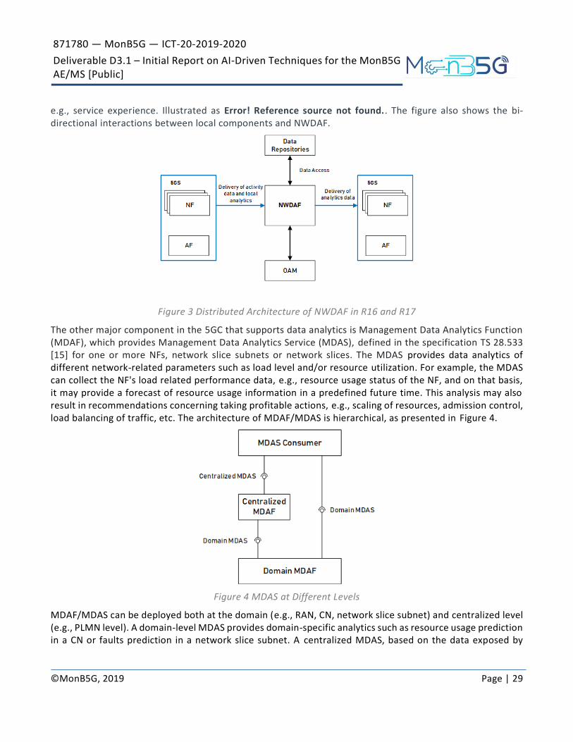
871780 — MonB5G — ICT-20-2019-2020


©MonB5G, 2019 Page | 29

e.g., service experience. Illustrated as Error! Reference source not found.. The figure also shows the bi-directional interactions between local components and NWDAF.

Figure 3 Distributed Architecture of NWDAF in R16 and R17

The other major component in the 5GC that supports data analytics is Management Data Analytics Function (MDAF), which provides Management Data Analytics Service (MDAS), defined in the specification TS 28.533 [15] for one or more NFs, network slice subnets or network slices. The MDAS provides data analytics of different network-related parameters such as load level and/or resource utilization. For example, the MDAS can collect the NF's load related performance data, e.g., resource usage status of the NF, and on that basis, it may provide a forecast of resource usage information in a predefined future time. This analysis may also result in recommendations concerning taking profitable actions, e.g., scaling of resources, admission control, load balancing of traffic, etc. The architecture of MDAF/MDAS is hierarchical, as presented in Figure 4.

Figure 4 MDAS at Different Levels

MDAF/MDAS can be deployed both at the domain (e.g., RAN, CN, network slice subnet) and centralized level (e.g., PLMN level). A domain-level MDAS provides domain-specific analytics such as resource usage prediction in a CN or faults prediction in a network slice subnet. A centralized MDAS, based on the data exposed by

871780 — MonB5G — ICT-20-2019-2020


©MonB5G, 2019 Page | 30

domain MDAF entities, can provide end-to-end or cross-domain analytics service covering resource usage or failure prediction in a network slice or optimal CN node placement, ensuring lowest latency in the connected RAN nodes.

4.1.2 ETSI ZSM

ETSI defines in its zero-touch service management (ZSM) framework a closed loop (CL)-based automation wherein the analytical function (AF) plays a pivotal role and is interfaced with several internal entities, including the data Collection Function (i.e., monitoring), the Decision Function as well as diverse external entities (authorized by ZSM). While the Collection Function is responsible for gathering and pre-processing data from managed entities (e.g., VNFs) or from external sources (e.g., context awareness positi onal data). In this respect, data might have different formats and be transferred from one or more sources (databases or streams) to a destination where it can be stored and further analysed. Since data has different origins, there is need for each source to be transformed in a way that allows it to be analysed in conjunction with data from other sources. The ‘Analysis’ Function is then responsible for deriving insights from available data from the collection stage as well as historical data. An insight is jointly extracted from data and the corresponding context. An example of insight may be the conclusion that congestion has taken place in a set of resources, and the context could be the location, time and date, the service impacted, users involved and the underlying set of slice resource. Insights can determine the root cause and locate it in the network. The insight derivation is therefore a continuous process that can be enhanced by new data. Analysis should be able to continuously improve its results and, consequently, provide better decision options to the decision function as depicted in Figure 5.

Figure 5 Functional View of a Closed Loop and its Functions within the ZSM Framework [16]

There are a series of interfaces defined in the ZSM framework. Specifically, the interfaces are introduced as:

871780 — MonB5G — ICT-20-2019-2020


©MonB5G, 2019 Page | 31

C2A interface between the Collection Function and the Analysis Function provides information based on historical and/or streaming real-time data coming from various data sources. Information is a set of data processed in a meaningful way following the goals assigned to the closed loop. The information derived from raw data is highly dependent on the context. Collection Function also supports features for (i) providing historical information, (ii) providing real-time information, (iii) tuning data sources, (iv) tuning data ingestion.

A2D interface between the Analysis Function and the Decision Function provides insights on historical and/or streaming real-time information that is provided by the collection stage. Analysis also provides capabilities for tuning the analytics models and starting/terminating the analytics processes.

E2 external interface represents data and control inputs and outputs from/to other closed loops and external entities and is used to (i) start/stop process of e.g., training an AI model, (ii) change the settings of the function such as the attributes of CL models, configurations that define how each CL works, (iii) retrieve the current status of the stage, (iv) retrieve the historical data and/or real-time data of the function such as logs, (v) provide the resulting data of the stage to other closed loops and (vi) provide data to authorized entities outside of the ZSM framework, e.g., external management system.

4.2 ML/AI Techniques for Data Analytics

Machine Learning techniques have proven very successful as function approximators [17] [18] to find solutions in different problem domains. A variety of Machine Learning methods have been employed to address data collected from different resources for diverse analysis tasks. Depending on the information available in the data itself and the problem to be solved, some approaches would be more feasible/efficient than others.

Supervised Learning, for example, is one type of ML methods in which the problems of classification and prediction are very important. The methodology to apply this type of learning requires data that is somehow labelled and the expected result is known from the data, in order to train a function approximator (which can be a Deep Neural Network) that can be used to label/classify/predict the outcome of never -before seen data inputs. Unsupervised Learning goes along similar lines, but in this type of ML the labels of the data and the expected output are not known, and the function approximator is left to determine this labelling on its own. A typical example of UL method could be the Principal Component Analysis (PCA).

Another family of ML methods is Reinforcement Learning (RL), in which an agent learns to perform an optimal action based on its inputs and a reward function that offers the agent a metric of performance. Even though RL has been mostly used for interactive settings between the agent and its environment, there have been state-of-the-art works that have formulated data analytics problems as Markov Decision Processes (MDPs) [19] [20] [21] [22], such that the advantages of the RL methods can be exploited to solve these problems.

4.2.1 TIME SERIES FORECASTING

The 5G architecture standard specifies the functionalities at each technological domain, their scope of programmability and the way they are managed [10] [23] [24]. Virtualization is key for deployment of network

871780 — MonB5G — ICT-20-2019-2020


©MonB5G, 2019 Page | 32

slices. This technology allows to decouple the infrastructure providers (InPs) from the service providers (tenants), which deploy and own the network slices.

The tenants get virtual resources depending on the needs of their slices, the VNFs and vi rtual links that compose it, and performance constraints usually defined in the form of SLAs. When a tenant deploys a network slice, the InP has to ensure there are enough resources available in the infrastructure for it [25]. Admitting a network slice into the infrastructure involves a process of assigning VNFs and their virtual links into their respective physical counterparts [25] [26].

4.2.1.1 RESOURCE ALLOCATION IN THE CONTEXT OF 5G

Upon slice admission, the tenant specifies the resources it needs for its slice(s), which may differ from its real usage. In the event a network slice needs more resources than those initially assigned, then it is under-provisioned. This causes the network slice to perform poorly, incurring in penalties for the InP and poor QoS for the end users [27]. In the opposite case, where the network slice uses less resources, then it is over-provisioned. In this case, resources remain idle but active incurring costs for the InP, and losing revenue. Over-provisioning also reduces the number of slices that can be simultaneously deployed, increasing the time for slices to be admitted, and also reduces the resource utilization efficiency of the infrastructure. Since both of these cases (over- and under- provisioning) imply costs for the InP and/or quality of service degradation for the end user, it is necessary to dynamically re-adjust the resources assigned to network slices [25].

In order to assess the amount resources to assign to a network slice, it is necessary to analyze its load [24]. Depending on the 5G technological domain, the type and management of resources will vary. In the base station at the RAN domain, the network slices need bandwidth for communication with user equipment, which is a limited resource. The InP maps and/or multiplexes the available bandwidth among the slices, in order to support a larger number of them [25]. Understanding the traffic profiles of each slice provides important information to achieve this target. Trying to predict the traffic becomes an attractive approach to drive bandwidth allocation mechanisms (and/or other resources) at the base station level [24] [28] [29].

4.2.1.2 TRAFFIC PREDICTION

There are many approaches for traffic prediction within the context of mobile communications [27] [30] [31] [32] [33] [34] [35]. ML techniques have been used as well, such as Linear Regression, Polynomial Regression, Gaussian Processes, Feed-Forward Neural Networks (FFNNs) communications [31] and more complex DNN architectures such as LSTMs and CNNs [27] [33] [34]. FFNNs and Autoregressive Integrated Moving Average (ARIMA) methods have similar performance for time-based prediction [36] [37], while LSTM-based predictors have shown better performance than ARIMA and FFNNs [38], and these have been proven very successful for traffic prediction [28] [33] [39] [40].

Most state-of-the-art ML predictors are trained with loss functions that minimize accuracy errors. However, there is a gap between the prediction and resource orchestration, and by focusing only on accuracy, the InPs use predictions that are agnostic to resource under- or over-provisioning. Thus, it is necessary to enhance the capability of predictors to reliably drive resource allocation and slice scheduling mechanisms.

871780 — MonB5G — ICT-20-2019-2020


©MonB5G, 2019 Page | 33

The Context-Aware Traffic Predictor (CATP), proposed as part of the data analytics engines developed within the MonB5G project, seeks to reduce the gap between traffic prediction and resource orchestration. Some aspects of CATP are similar to DeepCog [27], but CATP differs and extends from the latter by offering a formulation that injects problem domain as regularization terms of the loss function, and can be used to train different DNN architectures, leveraging supervised learning techniques for problem domain knowledge embedding when training DNNs [41] [42] [43].

4.2.2 CLASSIFICATION AND ANOMALY DETECTION

There are many types of anomalies that can be identified in a mobile communication network. These anomalies range from the simplest faults, such as links broken at the physical layer (broken wires or antennas), to application layer malfunctioning and system overload. This means that the scope of anomalies is very broad, and the patterns behind the anomalies are diverse. Thus, designing ML methods for anomaly detection requires to narrow down the context in which certain type of anomalies are expected.

In most cases, specific anomalies can be indirectly detected by observing the traffic load across the networks. When the traffic patterns change, or when there are spikes of traffic generating network congestion (considered an anomaly as well), then packet delivery drops, which is translated as a QoS degradation for the users.

Within this context, one of the main applications of traffic forecasting is to anticipate network congestion in order to implement automated mechanisms that help relieve the network of the congestion condition. A large part of these forecasting applications is done using time series forecasting [31] [44] [45] [46] [47] [48] [49] [50], but there are others that use other forms of Machine Learning [51]. Le et al. [31] argue that forecasting traffic load with a margin overload is effective in making congestion control more reliable when it is used with some form of resource provisioning to the network. On the other hand, Najm et al. [51] use a Decision Tree (DT)-based algorithm to determine whether congestion will occur or not depending on the conditions of the transport layer. Xie et al. [50] adopted a Deep RL approach to solve the congestion problem by determining the initial congestion window (IW), for which they use A3C (Asynchronous Advantage act or-critic) algorithm [52] [53] trained on flow completion time data. In the aspects of congestion control, we are in the process of developing a slice admission control strategy that considers traffic forecasting and resource allocation to determine the best slices to admit in order to reduce the probability of congestion. The predictor used are obtained using the CATP framework for traffic prediction design, also develop as part of the MonB5G project. Once the admission control strategy for congestion avoidance is developed, the next step will be to deploy a RL agent, similar to [50], to do fine-grain resource allocation to optimize the resource usage and prevent congestion even further.

4.2.3 GRAPH REPRESENTATION LEARNING

Graph data is pervasive in 5G networks. For example, the VNFs and virtualized links of a network slice construct a graph. To address such type of data, diverse ML methods have been explored. One of state-of-the-art methods is Graph Convolutional Networks (GCN), which generalize Convolutional Neural Networks (CNN) that only work on Euclidian objects, to arbitrarily structured graphs. Based on spectral graph theory, GCNs define the convolution operation of graphs using Chebyshev polynomials with trainable parameters

871780 — MonB5G — ICT-20-2019-2020


©MonB5G, 2019 Page | 34

that are learned in a neural network model. GCNs are used to automatically extract advanced features from graphs allowing to represent their semantics in a very effective way, as they encode and accumulate features of local neighbours.

The representation of graph features extracted by a GCN has been successfully used in recent works with different types of learning models such as semi-supervised classification [54] and Deep Reinforcement Learning [55]. However, GCNs can only be applied for representing homogeneous graphs, that is, graphs in which all nodes and all links are of the same type.

To deal with this limitation authors of [56] have developed a new technique called Relational Graph Convolutional Network (RGCN). The goal of RGCN is to extract features in heterogeneous graphs, where we have more than one type of node and link. This propriety is essential to learn appropriate representations of large-scale relational data graphs [56]. As GCNs, RGCNs accumulate transformed feature vectors of neighbouring nodes. However, RGCNs perform relation-specific transformations i.e., depending on type and direction of an edge.

4.2.4 FEDERATED LEARNING

Federated Learning is a recent Machine Learning paradigm that allows multiple agents to train a shared model in a decentralized manner without exchanging their local data. That means, with these techniques individual computing devices (potentially spread geographically) can come up with the same model that a single centralized server could find by gathering all their data, but without requiring as much storage capabilities or disclosing the data that each device holds.

Federated Learning emerged as a new way of exploiting the ever-increasing computing power at the edge of the network [57]. In particular, Federated Learning contrasts with "traditional" centralized Machine Learning model training in that it puts together elements from large-scale Machine Learning, privacy preservation and decentralized optimization, thus gathering and coupling the challenges of all these areas togeth er [58].

The main attractive features of Federated Learning are: (i) the distribution of the computing load into many individual devices instead of a unique server; (ii) the resilience of the decentralized approach versus mere parallelization, thanks to which even if any node suffers a failure the training can continue, as opposed to the case where a central node coordinates many parallel workers and if this node fails the training is interrupted ; and (iii) the exchange of model parameters instead of raw data, which allows for keeping the agent's local information private.

Current research on Federated Learning is dedicated to address many challenges caused by the standard centralized learning mode, namely:

1) Training a potentially huge model (neural networks can have millions of parameters) in a decentralized manner requires a large amount of communication. Current approaches to alleviate this drawback are trying to reduce the number of communication rounds [58] or the size of the messages transmitted [59].

2) Coping with the large heterogeneity of the devices and communication channels in the network. The very different storage capacity, computing power and communication reliability of the devi ces connected to the network require Federated Learning methods that are robust against lack or

871780 — MonB5G — ICT-20-2019-2020


©MonB5G, 2019 Page | 35

intermittent participation of certain agents. Current approaches to address this challenge are asynchronous communication, and accounting for the limited power of some components of the network instead of just ignoring them, which can have a negative impact on convergence [60].

3) The data collected at each device may differ significantly in their distribution, which on the one hand violates the assumption of independent and identically distributed (i.i.d.) data frequently used in distributed optimization, and on the other hand allows for the incorporation of other frameworks as multi-task learning [61].

4) A considerable challenge of Federated Learning lies in achieving a good trade-off between model performance and quality of the exchanged information, since even just exchanging the model parameters rather than the data itself can still reveal sensitive information [62]. Therefore, a great amount of effort is being dedicated to balance this trade-off to realize private federated learning systems.

Given the strengths of the Federating Learning framework (i.e., decentralized training and data privacy preservation), it is a natural choice for the implementation of the training of KPIs and SLAs predictors from the raw data collected locally at the analytic engines.

4.2.5 REINFORCEMENT LEARNING

According to [63], Reinforcement Learning (RL) is a family of ML methods that learn from interactions to achieve a goal. The reinforcement learning agent observers its environment – which comprises everything outside the agent, continually selecting actions to perform. The environment, responding to those actions, presents new situations to the agent and also rewards, special numerical values that the agent tries to maximize over time [63] [64] [65].

In an essential way, reinforcement learning problems are closed-loop problems because the learning system's actions influence its later inputs. A Reinforcement learning agent uses methods to discover which act ions yield the most reward by trying them out [63].

Reinforcement learning is different from supervised learning since supervised learning involves learning from a training set of labelled examples provided by a knowledgeable external supervisor. This is an important kind of learning, but alone it is not adequate for learning from interaction. In interactive problems it is often impractical to obtain examples of desired behaviour that are both correct and representative of all the situations in which the agent has to act [63].

Reinforcement learning is also different from unsupervised learning, which is typically about finding structure hidden in collections of unlabelled data. Uncovering structure in an agent's experience can certainly be useful in reinforcement learning, but by itself does not address the reinforcement learning agent's problem of maximizing a reward signal [63].

The book [63] classifies Reinforcement Learning methods in two macro-categories: (i) Tabular methods, and (ii) Approximate methods. Tabular methods adopt the strategy of building a model of the environment. The goal of these methods is to build a table or array containing an approximation of the action-value function – the function that represents the expected sum of rewards that can be obtained by taking an action from a specific state, for each possible state-action pair. The advantage of these methods is that they can often find exact solutions, that is, they can often find exactly the optimal value function and the optimal policy to select

871780 — MonB5G — ICT-20-2019-2020


©MonB5G, 2019 Page | 36

actions. However, they can only be applied in situations where the number of state and actions is sufficiently small to be represented in a table. Examples of Tabular methods are Dynamic Programming, Monte Carlo Methods and Temporal Difference Learning [63]. Approximate solution methods do not use tables to approximate value functions. They use instead function approximation strategies (e.g., artificial neural networks) to approximate the state value function and the policy. Optimality cannot be ensured but in return these methods can be applied effectively too much larger problems. Approximate solution methods can be divided in two categories: “On-policy” methods and “Off-policy” methods. On-policy methods are designed to learn an optimal policy while using it to select the actions made by the agent. Off -policy, in contrasts, train a policy different from the one used by the agent select the decision [63].Approximate methods do not use tables to approximate value functions. Instead, they use function approximation strategies (e.g., artificial neural networks) to approximate the state value function and the policy. Optimality cannot be ensured but in return these methods can be applied effectively to more complicated problems. Approximate methods can be divided in two categories: “On-policy” methods and “Off-policy” methods. On-policy methods are designed to learn an optimal policy while using it to select the actions made by the agent. Off-policy methods, in contrasts, train a policy different from the one used by the agent to select the decisions [63].

4.3 Solutions on Data Analytics Using ML/AI Techniques

The community has explored diverse ML/AI techniques for a variety of tasks in network management, e.g., network embedding, dynamic resource allocation, and admission control. This section will briefly summarize some of the works in the literature.

4.3.1 DRL APPROACH USING GRAPH CONVOLUTIONAL NETWORKS

Automatic virtual network embedding is an important task in network management and orchestration, and has attracted increasing attention due to high demand on zero touch management. Yan et al. [66] propose and implement a dynamic central online algorithm for automatic virtual network embedding by combining Deep Reinforcement Learning (DRL) with graph convolutional networks (GCNs). The algorithm automatically extracts spatial features in an irregular (non-structured) graph topology (i.e., the substrate network). For training the algorithm, a Policy Gradient method called "Asynchronous Advantage Actor-Critic (A3C)" [67] is used in the DRL model, where multiple instances of the training agent are curried out simultaneously which speeds up the process of learning.

The algorithm has considered CPU power for the substrate node and bandwidth for the inter-node links as the main physical resources constrains. The optimization objectives are to select and embed VNFs automatically taking into account the acceptance ratio, long term average revenue and running time. Embedded nodes then are connected by using the shortest path algorithm.

As the solution is DRL-based, the state is represented by the maximum available CPU and bandwidth resources on all SN nodes, free CPU power on each node, free bandwidth of every link on the SN, and also the required CPU and bandwidth by each virtual node in the VNR. The action by the algorithm is to embed the virtual nodes of the VNR and link them. This process is iterative and only terminates after all virtual nodes in the VNR are completely placed and linked. To evaluate each action of the algorithm, a reward function is

871780 — MonB5G — ICT-20-2019-2020


©MonB5G, 2019 Page | 37

used to encourage choosing successful actions. The reward function includes request acceptance ratio, long term revenue and load balancing.

4.3.2 DEEPVINE: VIRTUAL NETWORK EMBEDDING WITH DEEP REINFORCEMENT LEARNING

The recent advances of AI/ML about deep neural networks have been tailored and extended to solve the VNE problem. Dolati et al. [68] adopt a general Convolutional Neural Network (CNN) for a DRL to embed a virtual network (VN), i.e., a set of virtually linked VNFs. It is a dynamic, online, centralized solution for VNF placement. As DRL performs well on image classification and recognition, they assume that the physical and virtual networks have grid typologies as such they can encode them as two-dimensional images.

Those images are suitable to be directly fed to a deep neural network without any further processing. The DRL then selects an action upon which the image is updated and fed back to the neural network. The structure of this neural network has four convolution layers where the output of the last convolutional layer is divided between two fully connected layers and then merge in the last output. This "duelling" technique is proved to help learning better policies [69]. RL Q-learning algorithm is used as the training algorithm in this solution. Q-learning learns a value Q, called Q-value, for each state action pair which is equal to the maximum accumulated future reward when an action is performed in a state.

The reward function is designed to achieve a high cumulative value, which is maximized when the maximum number of VNs are embedded upon resources availability. After embedding a VN in a PN, a shortest path link is constructed between nodes and the state (image) is updated. There are four possible actions carried out by this solution: (i) mark VNs (and PNs) for embedding, (ii) perform the embedding, (iii) update marked VNs, and (iv) update marked PNs. To adhere to image representation in DRL, the state is represented using three matrices, which is a direct adaptation of the RGB colour channels in a coloured image. First, the matrix encodes the substrate network and the VN concatenation, it includes CPU and BW and their parameters. Second, the matrix uses the same encoding with embedded VN set to 1. Third, matrix is used to check resource availability. It is the same as matrix 1 but indicates whether an SN node or link has enough remaining capacity or not.

4.3.3 DRL-BASED DYNAMIC RESOURCE ALLOCATION (DRA) SCHEME

Dynamic resource allocation is enhanced with AI techniques to avoid or largely alleviate the resource under- and over-provisioning issues. The traditional method often sets a small utilization threshold. Resource will be scaled vertically or horizontally if the predefined threshold is reached. The simple method works; however, it often causes over-provisioning, and cannot fully exploit the resource of the infrastructure. The AI -based resource allocation dynamically optimizes the resource based on the actual demand, such that QoE is guaranteed, and on the other hand, more network slices can be supported in the same infrastructure. Wang et al. [70] develop a centralized, online DRL-based dynamic resource allocation scheme for networks slicing. They employ Deep CNN to model the complex 5G network environment. In this algorithm, features of SN are represented as a binary matrix to facilitate for the DRL agent to discover relations between multiple slices and learn to dynamically manage the resources of a slice depending on the perceived demands. It achieves resource optimization for all slices at once instead of individual VNFs.

871780 — MonB5G — ICT-20-2019-2020


©MonB5G, 2019 Page | 38

The DRL model consists of four convolutional layers, with two MaxPooling2D layers inserted after the second and the fourth convolutional layer. Rectified Linear Unit (ReLU) activation functions are used in all layers except the output. The output of the second pooling layer is flattened to one dimensional vector to be passed through a fully connected layer. SoftMax activation function is applied to the output for the purpose of probabilistic actions. The RL training agent uses Policy Gradient technique, called "RMSProp" [71], in training the network. A main component of the model is the scheduler which dynamically adjusts the allocated resources as a result of the actions produced by the training agent.

For state representation in the model, a four-dimensional tensor is constructed. The first dimension represents the resource requirements of a VNF for each type of resources. The second-dimension chains multiple VNFs of the same slice. The third dimension defines four key performance index of slicing resource management for each slice. These four-resource metrics are: resource allocation status of the VNFs of a slice on the physical nodes, the current resource usage of each VNF, the scale of the slice and the resource utilisation of the physical node. In the fourth dimension, all slice states are concatenated to produce the E2E model of the whole network. That tensor is directly applied as input to the agent as the environment state. The action generated by the agent informs the scheduler how to adjust the resources allocated to slices, then a scheduler might increase or decrease the resources of any VNF. To make the learning feasible and possible, the agent only affects one VNF at a time and keeps taking actions, in steps, until the resources of all the VNFs of each slice are updated.

The overall objectives of the solution are to minimize the SLA violations of slices, guarantee the performance and maximizing the resource utilisation of physical nodes. The DRL agent in this solution employs a reward function that depends on applying a penalty parameter for the SLA violation. It is calculated by summing the number of all VNFs in a slice that are allocated less resources than they require. The second parameter is the wasting penalty. This indicates the inefficient utilisation of resources which could lead to low revenue and energy waste.

4.3.4 ADAPTIVE DRL APPROACH FOR SERVICE FUNCTION CHAINS (SFCS) DEPLOYMENT

Xiao et al. [72] design and implement an adaptive online DRL approach, NFVdeep, to automatically deploy Service Function Chains (SFCs) to respond to different QoS requirement requests. NFVdeep is based on Markov Decision Process (MDP) model to capture the dynamic network state transitions. A Policy Gradient based DRL algorithm is adopted to improve the training efficiency and convergence to automatically deploy SFCs.

The NFVdeep constructs a fully connected multi-layer DNN with an input layer, an output layer and a variable number of hidden layers. The number of hidden layers is dependent on the number of nodes in the network. For example, if the number of nodes is less than 200, there will be 3 hidden layers and 4 layers otherwise. The layers are connected using ReLU and Tanh activation functions. The training agent of the model uses Policy gradient-based approach to enable automatic feature engineering and end-to-end learning. This proposed solution aims to capture real-time network variations and to apply an online SFC deployment solution. Those network variations are presented as state transitions to DRL. The main features considered are node resources (CPU and RAM) and link resources (bandwidth and latency). To train t he agent, the state is defined as a vector that represents: (1) the remaining physical resource of each PN and the remaining bandwidth of the Physical links, (2) the required resources and bandwidth by the currently processed VNFs,

871780 — MonB5G — ICT-20-2019-2020


©MonB5G, 2019 Page | 39

(3) the number of undeployed VNFs, (4) residual latency space, and (5) Time-To-Live (TTL) of the request. In training, the output of the agent is the node index, which represents the action. Each node is defined by an integral index. The VNF is placed with an index returned by the agent. The action 0 represents the case where the VNF cannot be deployed. If the action value is above 0, it indicates a successful VNF placement after which the system is updated and a new state is produced.

The main objects of NFVdeep are minimizing the operation cost of occupied servers for NFV providers and maximizing the total throughput of accepted requests for customers. As there is a need to jointly optimize different but related objectives, the reward function is defined as the total accepted requests (income) minus the total cost of occupied servers (expenditure) to deploy the arriving requests. The higher the value the better is the reward and vice versa.

4.3.5 DYNAMIC POLICY NETWORK BASED RL FOR VNE

Yao et al. [73] suggest an online, centralized and dynamic policy network based RL approach that extract features from the substrate network which serves as input to the policy network model. At the heart of the policy network is a convolutional layer which performs operations on the input to produce a vector representing the available resources. This vector is transformed by Softmax layer into the probability for each node. The outputs are a set of available substrate nodes with their probabilities for possible mapping.

In this solution the learning agent employs a Policy Gradient method for training. To enable the agent to choose the substrate nodes, features of each substrate node need to be extracted and used as input to the policy network. In general, the state the agent receives is represented as a feature matrix where each row is a feature vector of a certain substrate node. There are four features extracted from each substrate node, namely; CPU, the number of node connections (node degree), the sum of bandwidths of all links for that node, and the average distance to other host nodes (to calculate the cost). The optimization metrics are long-term average revenue, a long-term acceptance ratio, and a long-term revenue to cost ratio. Long-term revenue is the sum of CPU and bandwidth resource required by all VNs in a request. The cost is calculated by the consumption of the bandwidth on all links for the request, and finally the long-term acceptance ratio is the ratio of accepted requests to the total number of requests arrived. These metrics are applied during evaluation to evaluate the performance of this embedding algorithm.

The training agent uses a reward function which calculates the revenue to cost ratio of a single virtual request for every virtual node in this request. The gradient is only calculated on a successful mapping of VN request. On failure, no gradient is returned.

4.3.6 DRL IN MULTI-DOMAIN NON-COOPERATIVE VNF-FG EMBEDDING

Quang et al. [74] propose a DRL-based VNF-FG embedding approach in non-cooperative multi-domain context. Each domain employs a DRL agent to learn from history of its actions and rewards. In this approach, only one given client who is responsible for requesting VNF-FG embedding does the final mapping between the VNFs and the substrate nodes and links of the domains. As a non-cooperative approach, each domain does not have information of the topology and available resources of other domains. They do not communicate with each other and each domain only exposes the prices of then resources to the client, then the client makes a final decision based on these prices.

871780 — MonB5G — ICT-20-2019-2020


©MonB5G, 2019 Page | 40

At the heart of the DRL is an off-policy, actor-critic, Deterministic Policy Gradient (DDPG) [75] [76] algorithm which is used in the agent for training the network. DDPG uses two separate neural networks: the actor network which learns the policy, and the critic network which produces the Q-value to evaluate the action. In each domain there is a DRL agent that observes the state of that domain. An action is determined by the actor and its advantage is assessed by the critic network to improve the output. The client collec ts actions of domains which are called ’prices’, choose the best prices as the final action and executes it. For each domain a reward reflecting the resources provision to the client is calculated. Finally, the rewards are fed to the DRL agent to compute the loss and update the parameters of the DRL agent. The reward function is set to 1 only and only if the available resources are more than required and the QoS is satisfied. The requests are presented by the client of the VNF-FGs as the environment state. The state is primarily defined as a 3D-tensor where each dimension is a channel of N * N matrix where N is the number of VNFs in a request. The first channel is the required resources of the virtual links connecting VNFs in the request, which usually are bandwidth and latency. The other two channels are one for the source VNFs and the other one for the destination VNFs, and they represent the required resource in terms of CPU capacity, RAM and storage. Optimization decision is taken by the client depends on the resource prices that each domain offers. The price is calculated by summing the physical resources of all nodes of the substrate network as well as the sum of available link resources. They are presented to the client to select the domain with ’best price’ to do the embedding. In each domain there is a DRL agent that observes the state of that domain. An action is determined by the actor and its advantage is assessed by the critic network to improve the output. The client collects actions of domains which are called the ’prices’, choose the best prices as the final action and executes it. For each domain a reward reflecting the resources provision to the client is calculated. Finally, the rewards are fed in to DRL agent to compute the loss and update the parameters of DRL agent. The reward function is set to 1 only and only if the resources available are more than required and the QoS is satisfied. The requests are presented by the client of the VNF-FGs as the environment state. The state primarily defined as a 3D-array where each dimension is a Channel of N * N matrix where N is the number of VNFs in a request. The first channel is the required resources of the virtual links connecting VNFs in the request which usually are link bandwidth and latency. The other two channels are one for the source VNFs and the other one for the destination VNFs, and they represent the required resource in terms of CPU capacity, RAM and storage. Optimization decision is taken by the client depends on the resource prices that each domain offers. The price is calculated by summing the physical resources of all nodes of the substrate network as well as the sum of available link resources. They presented to the client to select the domain with ’best price’ to do the embedding.

In a summary, ML/AI based data analytics for 5G networks and for 5G network slicing has attracted increasing attention, and the related definitions have been integrated into the 3GPP and ETSI specifications. The current research results have demonstrated the potentials of ML/AI techniques. The slice-based network management generates a set of challenges related to scalability, security, automation in management of heterogeneous resources (e.g., communication, computational and storage), as well as to energy efficien cy without sacrificing performance. Earlier H2020 calls have already set a solid framework for the design of uniform network management and orchestration systems, (e.g., 5G!Pagoda, 5G-EVE, 5GENESIS and SliceNet), however, there are still open challenges to enable a scalable, proactive, energy efficient and secure slice lifecycle management, such as:

871780 — MonB5G — ICT-20-2019-2020


©MonB5G, 2019 Page | 41

Distributed management plane to support massive deployment of network slices.

Definition of novel end-to-end (e2e) slice Key Performance Indicators (KPIs) and development of AI-based mechanisms for their accurate prediction from multi-level metrics.

Data-driven management system based on federated learning.

Zero touch network configuration.

DE decisions tailored to the RAN.

AI-driven slice security management via robust and efficient trust-based mechanisms.

AI-driven energy efficient network management.

Beyond the state-of-the-art advances, MonB5G will develop distributed AI-based analytics entities in this work package (i.e., WP3) to fulfil the challenges 2, 3, and 5, in order to present a highly automatic framework for management of a massive number of co-existing network slices, together with the achievements of WP4 on Decision Engine and of WP5 on Security & Energy Enhancement. The current results of the WP about the distributed AI-driven analytics engine are reported in the sections 6, 7 and 8.

871780 — MonB5G — ICT-20-2019-2020


©MonB5G, 2019 Page | 42

5 MonB5G Monitoring System

In this section, we report the current progress of the distributed MonB5G monitoring system (MS). We have investigated state-of-the-art techniques for network monitoring, and explored the limitations of the existing systems and platforms. The results have been introduced in the section 3. Inspired by these findings, we propose the initial version of the distributed MS that is based on autonomic network management specifications and cloud-native design. The distributed MS is in line with the MonB5G architecture proposed in WP2, where MS is a sublayer of the slice management layer (SML) that is independent of the slice functional layer (SFL). There is an extra (embedded) element manager deployed at the VNF level, by which SML and SFL are connected. The distributed MS agents are designed to manage the tightest metrics sampling loops in its technological domain, such that the need for data transfer is largely reduced, and thus communication overhead of the monitoring system itself is minimized. The programmable sampling functions permit design of different aggregators for specific (e.g., slice-level) AE/DE.

5.1 Selection of Slice KPIs and Monitored Parameters

We first select informative metrics to be monitored with the MonB5G MS at different layers of the network management hierarchy. There exist thousands of heterogeneous metrics that can be used to observe the status of the technical domains and the network slices. Selecting most informative metrics is of practical importance, as useless features can cause unnecessary communication overhead and increase unexpected complexity of analytics engine. To identify relevant metrics, we establish a mapping between slice-level KPIs that are needed by AE and DE and the MS monitored metrics. A Slice KPI can be calculated by aggregating the measurements over all the underlying VNF/PNF components. In addition, we conduct in-depth analysis on the granularities of the selected metrics that facilitate the design of sampling functions and are vital to meet the time constraints.

To measure the MonB5G objective KPIs defined earlier in deliverable D2.2 [77], we select a set of network/slice-level KPIs and AI KPIs to monitor and analyse from a large number of candidates. While AI metrics are calculated by AE/DE and sent back to MS for storing them, network and slice-level KPIs are measured by MS directly, which are listed in the table below:

Table 4 Mapping between the High-Level Project KPIs and the Selected Slice-Level KPIs

High-Level Project KPIs Relevant Network/Slice/AI KPIs

[UC1/ES1 KPI-1]: Reduction of SLA Violations

SLA: End-to-end slice latency, Throughput, CPU, PRBs, connected users,

[UC1/ES1 KPI-4]: Reduce Overhead to the central system

Data volume exchanged between the local and central entities and Federated/Multi-agent learning KPIs

[UC1/ES1 KPI-5]: Support more NS instances

Number of admitted slices

[UC1/ES1 KPI-6]: OPEX reduction consumed energy, number of operations

871780 — MonB5G — ICT-20-2019-2020


©MonB5G, 2019 Page | 43

[UC1/ES1 KPI-7]: Reduce time to manage RAN resources

RAN reconfiguration delay

[UC1/ES1 KPI-8]: Improve slice performance isolation

Latency in the absence of orchestration, scheduling etc.

[UC1/ES1 KPI-9]: Reduce RAN-oriented overhead

MS Measurement frequency

[UC1/ES2 KPI-1]: Reduce the number of SLA performance violations by 20%

SLA: End-to-end slice latency, bandwidth, CPU, PRBs, connected users etc.

[UC1/ES2 KPI-2]: Improve network energy efficiency by a factor of 10

Consumed energy/bit/slice

[UC1/ES2 KPI-3]: Reducing Static Slicing overhead will result in 30% higher utilization (will be achieved with dynamic reconfiguration techniques)

Number of admitted slices with similar network configuration

[UC1/ES2 KPI-4]: Compared to Static Slicing, demonstrate the same or better SLA tolerances (or risk of missing SLAs) when dynamic slicing techniques are used

SLA: End-to-end slice latency, throughput, CPU, PRBs, connected users

[UC1/ES2 KPI-5]: 10x reduction in signaling / monitoring overhead with the use of federation techniques

Data volume exchanged between the local and central entities, and federated learning KPIs

[UC2/ES1 KPI-3]: E2e slice availability > 99%

Slice availability time/measurement period

[UC2/ES1 KPI-4]: Per slice component availability (probability that the service is available) > 99%

Component availability time/measurement period

We further define the identified network/slice/AI KPIs with detailed descriptions and introduce the commonly used manner to collect it. As depicted in the following table, the proposed distributed MS is designed to measure and store the following metrics at various discrete granularities. The granularities will depend on the requirements of both AE and DE, and could range between 1 min and 1 hour.

871780 — MonB5G — ICT-20-2019-2020


©MonB5G, 2019 Page | 44

Table 5 Slice-Level KPIs Description and Measurement

Metric Description Category Type Mapping to the Platform

Latency (control

plane (CP) and user

plane (UP))

Average E2E downlink packet delay between

Core cloud and UE Integrity Mean

End-to-end latency, regardless of CP/UP, needs to be explicitly measured. That is, MonB5G administrative elements should send control (timestamped) packets through such planes and compute delay. For the CP, MS are expected to serve as source/sink of such timestamped packets. UP delay estimations on the other hand would require UE to send these aforementioned control packets in order to accurately derive a latency estimation at the RAN, whereas latency in the UP at the Edge/Cloud TD can be derived by MonB5G administrative elements in a similar way as that in the CP.

Throughput Total packets Bytes in a granularity period

Integrity CumSum

Throughput can be derived from per-VNF telemetry. That is, by measuring the number of packets traversing VNF interfaces (e.g., leveraging EEM such as NetData) available throughput of the whole slice can be estimated accurately.

CPU usage CPU

consumption/Available CPU capacity

Usage Ratio

Per-VNF CPU and RAM consumption can be polled leveraging EEM (e.g., API exposed by NetData instance).

RAM usage RAM

consumption/Available RAM capacity

Usage Ratio

PRBs usage PRB

consumption/Total PRBs per slice

Usage Ratio With wireless SDN Controllers, the number of RB dedicated in the Uplink/Downlink direction can be queried/configured.

Number of admitted

slices

Number of slices successfully admitted

with resource allocation for SLA

Accessibility

CumSum With NFVO Northbound interfaces (e.g., Os-Ma), OSS/BSS (or other MonB5G administrative components) can request the number of running (or failed) network slice instances.

Connected users/slice

Number of RRC connected users per

slice

Accessibility

CumSum Users are directly mapped to UEs subscribed to a e/gNodeB. This metric can be extracted from the RAN management level (using its NBI), or from 4G vEPC or 5GC.

Slice end-to-end

availability time

Average time that slice VNFs are all

available

Retainability

Mean

Slice ‘readiness’ is announced by MonB5G administrative components to DMO via the domain shared messaging bus.

VNF/PNF availability

time

Average time that a VNF/PNF is not in fault

Retainabil

ity Mean

Reliability (Packet loss

rate)

Number of erroneous packets/total packets

per slice Integrity Ratio

Packets can be loss at the RAN or NFV segments of the Slice. Therefore, RAN controller’s NBI and VNF-instances’ telemetry API (i.e., EEM) are exploited to compute this metric.

871780 — MonB5G — ICT-20-2019-2020


©MonB5G, 2019 Page | 45

Data volume exchanged

between the local and

end-to-end entities

Total bytes exchanged between local and end-to-end entities

Integrity CumSum

MonB5G administrative components should keep account of Requests/Responses as well as Publish/Subscribe operations among technological domains. This bookkeeping can be queried directly via their respective NBI, serving as input to the computation of this metric.

Consumed energy

Average power consumption in a granularity period

Integrity Mean Initially expected to be the result of computations which take CPU/RAM consumption as base metric.

Number of operations

Total slice life-cycle management operation in a

granularity period

Integrity CumSum At Network Slice Instance level, this metric can be queried leveraging NFVO NBI. Such operations may include: VNF placement, scaling, termination, etc.

5.2 Architecture of MonB5G MS

MonB5G MS is conceived as a cross-domain virtual layer hosted by a NFV IFA 029 compliant PaaS (i.e., Container Infrastructure System (CIS)). This can be mapped to the Slice Management Layer (SML) or MonB5G Layer as a Service (MLaaS) concepts proposed in the MonB5G architecture in Deliverable 2.1 (D2.1). Figure 6 illustrates the overall architecture of the MonB5G monitoring system.

Figure 6 Architecture of the MonB5G Monitoring System

SML/MLaaS resources are orchestrated alongside the Slice Functional Layer (SFL), which hosts the managed components (e.g., tenant slices’ components) per Slice Orchestration Domain (SOD). That is, an end -to-end slice hosting functional components at the RAN, Edge and Cloud Technological Domains (TD) (i.e., Network

871780 — MonB5G — ICT-20-2019-2020


©MonB5G, 2019 Page | 46

Slice Service Instances (NSSI)) shares system resources with its corresponding SML/MLaaS instance. The proximity of SFL and SML/MLaaS in an SDO reduces network delays and inter-domain management traffic, allowing the creation of tight Closed Control Loops (CCLs) (e.g., instances of ETSI ZSM approach) at each TD. MonB5G proposes nesting CCLs per TD, i.e., VNF/PNF, Slice, and OSS/BSS. From a MS perspective, this implies different monitored elements and monitoring data consumers or requesters.

Figure 7 provides an overview of the envisioned interactions involved in the request and retrieval of metrics via MonB5G MS. Particularly, it depicts a generic Requester (e.g., AE/DE hosted in a TD at the same or higher level) pushing a Sampling Loop1, which allows MS NBI to redirect a specific request to a precise Manager instance (e.g., in a particular TD). The MS Manager instance thus delegates Sampling Loop Orchestration and Life Cycle Management (LCM) to the CIS. Figure 7 also depicts generic Sampling Loop Operations, which include (a) metric sample collection from a Monitored Element NBI (i.e., Embedded Element Manager (EEM)), (b) sample processing (e.g., an operation, caching), and (c) registering. The latter may occur via publishing the result of (b) in a corresponding message bus (e.g., Kafka topic), or appended to a Time Series Database (TSDB) (e.g., InfluxDB, MongoDB, and Prometheus). Conversely, (a) and (b) operations are executed by Sampling Functions (SF), which are particular for each EEM or monitored element.

Under the aforementioned paradigm Sampling Loops can be conceived as 1) periodic executions of Sampling Loop Orchestration + Operations managed by the CIS, or 2) a single execution with embedded configuration to ensure sufficient sampling resolution. This separation is rooted in CIS limitations on orchestrating Sampling Loops with periods lower than one minute. If mapped to CIS workloads, type-1 Sampling Loops are realised as Kubernetes CronJobs, while type-2 are standard Deployments. This is exemplified in Figure 8.

1 E.g., Kubefed (https://github.com/kubernetes-sigs/kubefed), Ingress (https://kubernetes.io/docs/concepts/services-networking/ingress/)

https://github.com/kubernetes-sigs/kubefed

https://kubernetes.io/docs/concepts/services-networking/ingress/

871780 — MonB5G — ICT-20-2019-2020


©MonB5G, 2019 Page | 47

Figure 7 MS Request and Metrics Retrieval from Monitored Element

Sampling Loop configuration files should follow MonB5G information model for MS. That is, it is a configuration file to a well-known API designed to handle the range of configurations supported by MS (e.g., CIS workload type, TD, sample retrieval method, etc.). Furthermore, CIS workloads require Sampling Functions to be conceived as Docker images that admit configuration parameters via predefined environment variables. The case of higher-TD MS follows directly from Figure 7, but Requester may only retrieve from Storage/Msg. Bus e.g., in order to serve AE tailored to slice-wide or cross-domain analysis.

871780 — MonB5G — ICT-20-2019-2020


©MonB5G, 2019 Page | 48

Figure 8 Mapping Sampling Loop Orchestration to Implementation Tools

MS enables the workflow described in Figure 7. Flexibly, it allows Sampling Function to be agnostic of the technology used for Sampling Loops Admission Control and Orchestration, instead dedicating their focus on Loop Operations only.

5.3 Domain-specific MS

This subsection introduces in more details development of the distributed monitoring system at different technological domains as well as the motivations behind the implementation mechanism. For the domains of RAN, Edge and Cloud, we illustrate the locally deployed cloud-native MS entities with comprehensive discussions on their technical KPIs, including collection granularity, efficiency and cost of computation and storage, overhead of communication. Although the MS entities are distributed in different technological domains, they are designed as a whole for zero-touch management and orchestration using the MonB5G platform. The domain-specific MS entities follows the key norms and concerns as below:

Stay in line with the MonB5G framework and the target KPIs (see details in MonB5G Deliverable 2.1-2.2)

Fulfil the functionalities, including data collection, aggregation, data pre-processing and storage

Implement different granularities for non-real-time and near-real-time intelligent control

Promote flexibility of MS entities, which activities are triggered and configured by AEs and DEs

Foster scalability and efficiency, e.g., communication overhead reduction

For all MS entities distributed in the different technological domains, the principal consumers of the collected metrics are AEs. After triggered and configured by AEs, the programmable MS entities connects the

871780 — MonB5G — ICT-20-2019-2020


©MonB5G, 2019 Page | 49

corresponding infrastructure and network functions (VNFs and PNFs) to collect the requested telemetries with the defined granularity. There are mainly three types of APIs associated with each MS entities, incl uding Control API, Data Collection API, and Data Processing API. The MS Control API decides the data source, the metrics to be monitored, the sampling frequency, the data format as well as the communication manner (e.g., publish/subscribe and request/response). The Data Collection API is the interface from which data are provided as AEs requested through the Control API. The Data Processing API is in charge of data filtering, aggregation, normalization etc. In the following subsections, we will provide more details of the domain specific MS entities.

5.3.1 MS IN THE RAN DOMAIN

The MonB5G monitoring system inspecting the RAN domain (MMS-RAN) is shown as Figure 9. It constitutes MS-sublayer of the SML for the RAN domain, and consists of the following functional components:

Monitoring manager (MM) is responsible for lifecycle management: trigger, manage and delete a monitoring task. It also supports remote configuration of the MS operations.

Monitoring data collector (MDC) connects with the RAN management and orchestration system to collect detailed real time metrics of eNB/gNB. Additionally, the RAN orchestrator is associated with a Netdata instance (https://www.netdata.cloud/) to collect other requested metrics, such as health and performance statistics of the containers of the RAN management system. Netdata empowered MDC provides fine granularity and high scalability for data collection. In the MonB5G platform, Netdata plays a role of MAPE-based Embedded Element Manager (EEM) that is implemented as a component of the corresponding functional entity (VNFC).

Monitoring data processor executes data pre-processing function defined by the requirements of the analytics engine, such as aggregation, filtering and normalization. This helps further reduce communication and computation overhead.

Monitoring database (optional) is utilized to store the pre-processed telemetries. The saved historic data facilitates improving performance of the AI models used in AEs and DEs. To keep aligned with open-source MANO (https://osm.etsi.org/), Prometheus (https://prometheus.io/) could be a choice to record the metrics. Since some features of Prometheus are not necessary in the case, it is also possible to directly adopt Gnocchi (https://gnocchi.xyz/) as a lightweight solution.

Event alert & visualization (optional) is a function to directly report alarms based on pre-defined thresholds and visualize the collected telemetries in dashboards, e.g., Grafana (https://grafana.com/).

MS-bus aims to handle streaming data feeds among the aforementioned components. The publish/subscribe tools, such as Kafka (https://kafka.apache.org/), can be employed for a unified, high-throughput and low-latency communication.

https://www.netdata.cloud/

https://osm.etsi.org/


https://gnocchi.xyz/

https://grafana.com/

https://kafka.apache.org/

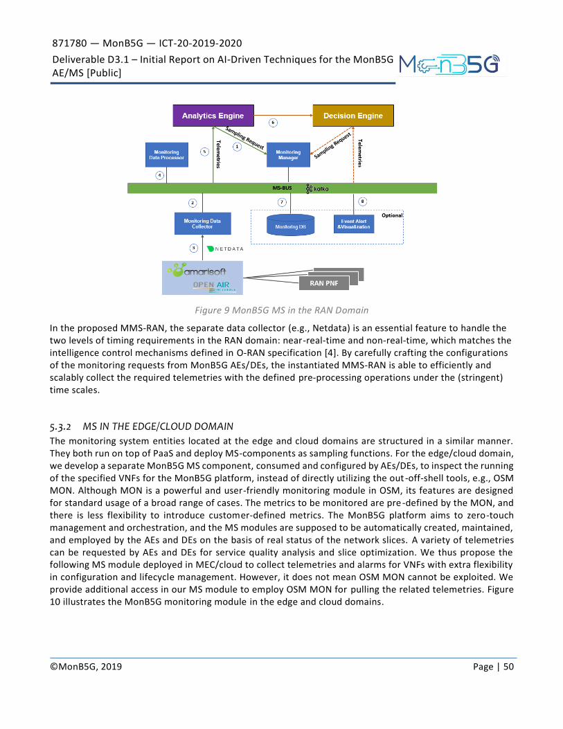
871780 — MonB5G — ICT-20-2019-2020


©MonB5G, 2019 Page | 50

Figure 9 MonB5G MS in the RAN Domain

In the proposed MMS-RAN, the separate data collector (e.g., Netdata) is an essential feature to handle the two levels of timing requirements in the RAN domain: near-real-time and non-real-time, which matches the intelligence control mechanisms defined in O-RAN specification [4]. By carefully crafting the configurations of the monitoring requests from MonB5G AEs/DEs, the instantiated MMS-RAN is able to efficiently and scalably collect the required telemetries with the defined pre-processing operations under the (stringent) time scales.

5.3.2 MS IN THE EDGE/CLOUD DOMAIN

The monitoring system entities located at the edge and cloud domains are structured in a similar manner. They both run on top of PaaS and deploy MS-components as sampling functions. For the edge/cloud domain, we develop a separate MonB5G MS component, consumed and configured by AEs/DEs, to inspect the running of the specified VNFs for the MonB5G platform, instead of directly utilizing the out -off-shell tools, e.g., OSM MON. Although MON is a powerful and user-friendly monitoring module in OSM, its features are designed for standard usage of a broad range of cases. The metrics to be monitored are pre -defined by the MON, and there is less flexibility to introduce customer-defined metrics. The MonB5G platform aims to zero-touch management and orchestration, and the MS modules are supposed to be automatically created, maintained, and employed by the AEs and DEs on the basis of real status of the network slices. A variety of telemetries can be requested by AEs and DEs for service quality analysis and slice optimization. We thus propose the following MS module deployed in MEC/cloud to collect telemetries and alarms for VNFs with extra flexibility in configuration and lifecycle management. However, it does not mean OSM MON cannot be exploited. We provide additional access in our MS module to employ OSM MON for pulling the related telemetries. Figure 10 illustrates the MonB5G monitoring module in the edge and cloud domains.

871780 — MonB5G — ICT-20-2019-2020


©MonB5G, 2019 Page | 51

Figure 10 MonB5G MS in the Edge/Cloud Domain

The essential functions of the MS components, such as monitoring manager and monitoring data processor , are implemented similarly as the ones for the RAN domain. The major differences focus on the component of the monitoring data collector. For the edge/cloud domain, each instantiated VNF is associated with a Netdata instance. When an AE requests telemetries of specific VNFs for analysis, the monitoring data collector activates the corresponding Netdata instances to provide the telemetries based on the configurations defined by the AE. Moreover, the monitoring data collector is also featured to connect OSM MON as well as VIM’s telemetry services (i.e., OpenStack’s Gnocchi in our case) for metrics collection. The MS is structured as a sublayer located in the slice management layer of the MonB5G platform, and all the FCAPS functionalities can be dynamically deployed or updated during slice lifetime using the orchestration capabilities of Inter-Slice Management (ISM), which also support the MS with the resource scaling mechanism.

In a summary, the domain specific MonB5G MS entities follow the concept of Slice Management Layer (SML) as a Service proposed in the MonB5G architecture in Deliverable 2.1. The distributed MonB5G MS collects the operation status at multiple levels of the management hierarchy (node, slice, domain, and inter -domain) as a sublayer of the SML. After triggered and configured by AEs, the programmable MS entities connects the corresponding infrastructure and network functions (VNFs and PNFs) to gather the requested telemetries with the specific granularity defined by the AEs. The distributed MonB5G monitoring system achieves the following advantages. First, the distributed MS agents are designed to manage the tightest metrics sampling loops in the respective technological domain, such that the need for data transfer is largely reduced, and thus communication overhead introduced by the monitoring system itself is minimized. Additionally, an extra MAPE-based embedded element manager is deployed at VNF level to support fine granularity (1s) of telemetry collection. It also permits development of aggregators for specific (e.g., slice -level) AE and DE. More importantly the configurations of MS entities distributed at different technical domains are automatically defined and triggered by the AE/DE components with AI-assisted policy-driven mechanisms, which take a crucial step towards highly automated slice-level monitoring system.

871780 — MonB5G — ICT-20-2019-2020


©MonB5G, 2019 Page | 52

5.4 Cooperation of MS with AE and DE

The traditional centralized network management constitutes a bottleneck and is not scalable in case of a massive number of network slices as expected in beyond 5G and pre-6G cellular systems. While centralized approaches could benefit from a holistic view of the whole network, they provide poor scalability when dealing with realistic scenarios, and introduce a significant monitoring overhead. Therefore, distributed management techniques are mandatory to: i) minimize the exchange of information in the network, ii) guarantee scalability of the overall slice management system and, iii) reduce the latency. As a distributed system, the interfaces between different entities would be more complicated, and need to be defined clearly. The aim of this section is to provide an overview of the communication links and the interactions between the (local/central) MS and the AE and the DE blocks proposed in the context of MonB5G.

Figure 11 shows the way the MS, AE and DE are expected to communicate with each other. This figure also includes the actuators which translate DEs decisions into API calls to different slice components (e.g., VNFs, links, PNFs) in each of the technological domains (RAN, Edge, Cloud) that a slice is supposed to cross.

Figure 11 MS Interfaces

The MS in Figure 11 is the one responsible for gathering a set of different metrics from the systems that the DE is controlling. This information can be passed to the DE and the AE directly, but they are also stored in a common online memory store (COMS), illustrated by the grey cylinder. This COMS is added in order to avoid implementing hard synchronization constraints among the MS, DE, AE whenever information needs to be exchanged. In this way, the DE and AE can be more flexible in terms of the length of their processing without compromising the granularity at which the MS can sample monitoring data from the controlled systems. So, it is the MS (depending on its capabilities and amount of information as well as the granularity set from the External User Interface (EUI)) that somehow defines how fast the data is sampled . It is worth emphasizing that COMS is in line with the ‘Knowledge’ block of the ETSI ZSM functional scheme presented in Figure 5. Furthermore, it should be noticed that the COMS block is controlled by the MS, but this does not mean that

871780 — MonB5G — ICT-20-2019-2020


©MonB5G, 2019 Page | 53

the MS only includes the memory (it includes the bus, the database, etc.). The COMS can be either a Time Series Data Base (TSDB) or an in-memory database.

The AE then reads the monitoring information from the COMS in order to pre-process it (e.g., perform predictions) before making it available to the DE. The AE may also read information directly from the MS, but this is expected to be used in more punctual cases, where synchronization is needed. The prediction interval can also be set from the EUI. Once the AE outputs the pre-processed data, it will proceed to store it in the COMS.

In a similar way, the DE is expected to read its input from the COMS, however it is also possible to receive this information directly from the AE and MS. Once the DE has generated its decisions, it will also store those in the COMS, as well as issue them to the actuator interfaces of the systems to translate them into API calls for slice components lifecycle management (LCM). DE parameters can be fine-tuned in runtime from EUI as well and might take effect in the next DE configuration update interval. The table below provides a description of the different interfaces that link MonB5G DE with the other control blocks.

Table 6 MS Interfaces and the Associated Roles

Interface Type Role

IMD Tensors/Database query

DE reads raw MS measurements (either online or from COMS)/Store AI metrics and DE decisions in COMS

IMA Tensors/Database query

AE reads raw MS metrics/Store AI metrics, predictions in COMS

IUM Database Query EUI reads/changes MS configuration (e.g., granularity)

871780 — MonB5G — ICT-20-2019-2020


©MonB5G, 2019 Page | 54

6 MonB5G AE Vision

6.1 AE Structure and Interfaces

As show in Figure 12 MonB5G Analytics Engine (AE) has been designed to contain two main functions, namely, KPI prediction and fault detection, and exploits MonB5G distributed architecture to push the analysis close to the data collection Monitoring Systems (MS) in each domain (i.e., RAN, Edge and Cloud), minimizing the need to transfer raw slice performance and configuration data across the different network domains and slices. As will be shown in the developed solutions, this will lead to a dramatic reduction in the communication overhead and yields more scalability in managing a massive number of slices.

6.1.1 KPI PREDICTION

This function mainly consists of the following two modules:

Time-series prediction of slice-level metrics such as the traffic and resource usage in order to help the Decision Engine (DE) taking preventive actions against e.g., Service-Level Agreement (SLA) violations. To that end, time-series prediction leverages customized and fine-tuned serial architectures such as Long Short-Term Memories (LSTM) and other advanced variants.

Parameters’ space prediction that aims at establishing accurate models to link certain measured input metrics (e.g., traffic per slice, channel quality, CPU load) with a target output metric (e.g., energy consumption per slice) while ensuring a certain SLA requirement. This type of analysis will guide the DE to fine-tune its action space, where it can know the order of magnitude/interval of the action to achieve e.g., a low SLA violation rate. To that end, AE is intended to adopt a new class of statistical/constrained neural networks/models, among other techniques.

6.1.2 FAULT DETECTION

The role of this function is to detect abnormal events during a slice l ifecycle, by mainly extracting and recognizing changes in data distributions and trends. This relies on advanced techniques of clustering and classification with e.g., novel architectures of neural networks. Since network slices are typically software and virtualization-based, the notion of fault includes but is not limited to the failures of the infrastructure on top of which the slice is running. Specifically, a slice fault could be a logical abnormality where, e.g., the classification of slice traffic (inspired by deep packet inspection) reveals that it does not fit into the slice predefined template, and therefore the isolation is breached.

Figure 12 Local AE Functions

871780 — MonB5G — ICT-20-2019-2020


©MonB5G, 2019 Page | 55

6.1.3 AE INTERFACES WITH MS AND DE

Figure 13 shows the way the AE on one hand and MS, DE on the other hand, are expected to communicate with each other. The figure also includes the interfaces between other MonB5G management components, and the actuators which translate DEs decisions into API calls to different slice components (e.g., VNFs, links, PNFs) in each of the technological domains. (The figure looks the same as Figure 11, as all interfaces are illustrated to give a complete picture of the interactions of the blocks.)

Figure 13 AE Interfaces

The MS is the one responsible for gathering a set of different metrics from the systems that the DE is controlling. The information can be passed to the DE and the AE directly via a messaging bus, e.g., Kafka, but they are also stored in a common online memory store (COMS), illustrated by the grey cylinder. This COMS is added in order to avoid implementing hard synchronization constraints among the MS, DE, AE whenever information needs to be exchanged. In this way, the DE and AE can be more flexible in terms of the length of their processing without compromising the granularity at which the MS can sample monitoring data from the controlled systems. So, it is the MS (depending on its capabilities and amount of information as well as the granularity set from the External User Interface (EUI)) that somehow defines how fast the data is sampled. It is worth emphasizing that COMS is in line with the ‘Knowledge’ block of the ETSI ZSM functional scheme presented in Figure 5.

The AE then reads the monitoring information saved in a common online memory store COMS located inside

the MS block (in order to avoid implementing hard synchronization constraints) to analyze it (e.g., perform

predictions) before making it available to the DE. The AE may also read live measurement information directly

from the MS, but this is expected to be used in more punctual cases, where some synchronization is needed.

The prediction interval can also be set from the EUI . Once the AE outputs the analysis results, e.g.,

predictions of traffic load and resource usage, it will proceed to store it in the COMS as well.

871780 — MonB5G — ICT-20-2019-2020


©MonB5G, 2019 Page | 56

Table 7 provides a description of the different interfaces that link MonB5G AE with other management blocks.

Table 7 AE Interfaces and the Associated Roles

Interface Type Role

IAD Tensors/Database query

DE Reads the predicted KPI from AE (either online or from COMS)

IMA Tensors/Database query

AE reads raw MS measurements, and store AI metrics, predictions in COMS

IUA Database Query EUI reads/changes AE configurations

6.2 AE Cross-Domain Operation

The MonB5G concept is based on taking advantage of local, distributed predictors in building accurate slice -level KPI prediction and fault detection. This concept brings in certain advantages, but also comes with costs that must be taken into consideration.

Training domain-specific distributed predictors may require using all the data collected at each slice.

However, privacy-preservation might impose the constraint of keeping the data private. Decentralized

Optimization techniques provide powerful tools to perform the training in a distributed manner without

sharing the data owned by each slice.

A simple example of such methods is shown in Figure 14. Panel a) shows the data of a 6-node network to fit a linear regression model. The color dots show the data at each node, and the full lines in color the best model parameters that each node would find in isolation. The dash-dot lines show the parameters estimated at each node at the end of the optimization process, and the red dashed line the optimal mode parameters if the problem was solved in a centralized manner (which would require the nodes to send the data to the central location).

In this example, all nodes depart from the optimal model parameters that they would find in isolation , instead, find the model that best fits the totality of the data. The final solutions at each node after a few iterations of the algorithm are extremely close to the analytic solution found considering all the data. The configuration of the network plays a role in the speed at which the error from the optimum decreases, as shown in panel d).

871780 — MonB5G — ICT-20-2019-2020


©MonB5G, 2019 Page | 57

Figure 14 Example Application of Decentralized Model Training. a) Data at Each Node; b) and c) Two Different Network Topologies; d) Difference in the Convergence Speed

The same mechanism can be applied to learn predictors of the state of the entire network using the data

collected at the analytic engines in each domain, and there is no requirement of the individual slices sharing

their (private) data.

The following advanced AI techniques will be explored and extended to instantiate MonB5G architecture, such that the decentralized AEs at different domains and slices are capable of collaborating to yield accurate prediction and detection:

Customized federated learning (FL) approaches, where the local AEs share their models, instead of raw data, with the E2E AE that performs particularly model aggregation and broadcasts it to the local AEs as depicted in Error! Reference source not found..

Distributed models, where the model layers located in different AEs as show in Figure 16.

Both classes of approaches will be further exploited in the proposed solutions reported in the next sections.

871780 — MonB5G — ICT-20-2019-2020


©MonB5G, 2019 Page | 58

Figure 15 Cross-Domain AE Cooperation via Federated Learning

Figure 16 Cross-Domain AE Cooperation via Distributed NN

871780 — MonB5G — ICT-20-2019-2020


©MonB5G, 2019 Page | 59

7 MonB5G Analytics Engine for Slice-Level KPI Prediction

Slice-level KPI prediction is crucial in supporting proactive management of network slicing. Slice-level KPIs can be related to ensuring SLAs or to ensuring that the system works within certain parameters that we require. These predictions are consumed by the decision engine (presented in Deliverable 4.1) to enable correct run-time decisions about dynamic slicing. The slice-level KPIs that will be predicted are presented in Table 5. Please note that we do not aim to predict all slice-level KPIs, but instead will choose the ones that will be directly related to our final use cases.

Our solution will encompass several prediction methods, as described in the following sections, which are part of the AE component. Several relevant issues are investigated through various approaches:

In Section 7.1, we discuss local prediction, the advantages and the cost of using distributed predictors, and we give an example of a case where we use a distributed LSTM algorithm to predict traffic over a set of base stations in the RAN domain.

In Section 7.2, we present a novel method termed statistical federated learning to predict resource usage while ensuring pre-defined SLA violation rate.

In Section 7.3, we present an approach of taking the network context into account during prediction, as seen through the lens of defining the costs associated with under- and over-provisioning. A second approach is described through a split architecture for the predictor between the RAN and MEC domains, with the lightweight RAN predictors giving quick local predictions, while the MEC -based predictions can be used when we need a better accuracy from the predictor.

7.1 Local KPI Prediction

One interesting research direction that we investigated is the idea of collecting traffic load measurements

from all BSs in the RAN domain of the network, and then gathering them in a central AE where we do the

training. Then we send to all BSs the weights of the NN model as exported by the training process. For service

time, each BS can directly use the pre-trained model to make predictions. Importantly, as the inference has

to be carried out in a BS, the model needs to be lightweight, that is fast in terms of inference, and not very

hardware demanding.

To this end, here we explore the application of long-short-term memory (LSTM) NNs for the problem of

predicting the traffic intensity (otherwise called load or demand) measured in MBs in time. Using such

recurrent neural networks is a natural approach for tasks involving time-series data. Essentially, we are

interested in the problem of resource prediction for each BS in the RAN domain of the network. A fitting

dataset for our problem is the Milano dataset, as it includes “Internet traffic in MBs” for a variety of BSs

placed in a geographical area. Please refer to the section 3 for more details of the dataset. Our first attempt

to tackle the problem is, for all BSs in the network, to split the time series dataset in windows of W time

instances, and use this as our input X = [S(t-W), …, S(t)], the input of the LSTM model, and then to require

from the NN model to be as close as possible to the next time instance, i.e., y = S(t+1).

871780 — MonB5G — ICT-20-2019-2020


©MonB5G, 2019 Page | 60

Figure 17 Vanilla LSTM Neural Network. Left: Lag Signals (Inputs). Right: Predicted Signal of the Next Time Instance (Outputs)

We then make batches from various BSs (X, Y) pairs and feed it to the NN. Interestingly, this task proves to

be relatively hard for the LSTM, and LSTMs with low memory size (<10) even failed to converge in terms of

training loss. In the figure below, we can see that the models with large memory size (20, 50, and 100) manage

to converge in terms of training loss.

Figure 18 Training Loss vs Epochs for Vanilla LSTMs with Different Memory Sizes

To this end, we decided to depart from this over simplistic approach of using only the in/out signals, we

augment the input vector with additional information, that is: (a) BS id, (b) day of the week, and (c) time of

the day. This extra information is the so-called “embedding”, which essentially acts as some sort of encoding

that further refines the LSTM’s understanding over the I/O signals we feed it. The new NN is shown as follows:

871780 — MonB5G — ICT-20-2019-2020


©MonB5G, 2019 Page | 61

Figure 19 Enhanced LSTM Neural Network with Traffic and Meta Information as Inputs to Predict the Traffic of the Next Time Instance.

We observed that this NN training loss performance converged well even for very light (low-memory) models.

Below we can see some results from the training process, more specifically the training error along with the

epochs, for different values of memory sizes.

Figure 20 Training Loss vs Epochs for Enhanced LSTMS with Meta Data, Tested with Different Memory Sizes

We then test this enhanced model, and “deploy” (in a simulation environment) it in different BSs. Right

below, we see with blue, the true value of the traffic demand of some BSs, and with orange, we see the

871780 — MonB5G — ICT-20-2019-2020


©MonB5G, 2019 Page | 62

predicted ones. It demonstrates that indeed we can achieve quite high accuracy, by deploying this lightweight

model across many different BSs in the RAN domain.

Figure 21 Traffic Intensity (Prediction and Ground Truth) for 6 Different BSs

7.2 Cross-Domain KPI Prediction

To minimize network overhead at the RAN/edge/cloud domains, dynamic resource usage prediction for network slicing can leverage advanced federated learning (FL) techniques. In this subsection, a new approach termed Statistical Federated Learning (SFL) for low overhead analytic engine (AE) is presented, which can learn resource usage models over a data distribution in an offline fashion while respecting some predefined local service level agreement (SLA) constraints defined in terms of long-term statistics over an observation window. The focus here is on resource cumulative distribution function (CDF)-based SLA---that is also dataset-dependent and nonconvex non-differentiable---and the corresponding SFL local optimization task is formulated using the proxy-Lagrangian framework and solved via a non-zero sum two-player game strategy. Numerical results show that the proposed decentralized AE resource provisioning approach enables SLA enforcement while significantly reducing the communication overhead compared to a centralized setup at the expense of a short delay.

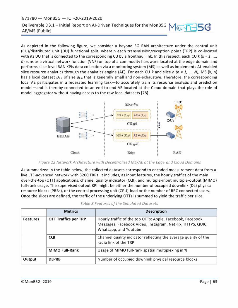
871780 — MonB5G — ICT-20-2019-2020


©MonB5G, 2019 Page | 63

As depicted in the following figure, we consider a beyond 5G RAN architecture under the central unit (CU)/distributed unit (DU) functional split, wherein each transmission/reception point (TRP) is co-located with its DU that is connected to the corresponding CU by a fronthaul link. In this respect, each CU k (k = 1, ..., K) runs as a virtual network function (VNF) on top of a commodity hardware located at the edge domain and performs slice-level RAN KPIs data collection via a monitoring system (MS) as well as implements AI -enabled slice resource analytics through the analytics engine (AE). For each CU k and slice n (n = 1, …, N), MS (k, n) has a local dataset Dk,n of size dk,n that is generally small and non-exhaustive. Therefore, the corresponding local AE participates in a federated learning task—to accurately train its resource analysis and prediction model—and is thereby connected to an end-to-end AE located at the Cloud domain that plays the role of model aggregator without having access to the raw local datasets [78].

Figure 22 Network Architecture with Decentralized MS/AE at the Edge and Cloud Domains

As summarized in the table below, the collected datasets correspond to encoded measurement data from a live LTE-advanced network with 3200 TRPs. It includes, as input features, the hourly traffics of the main over-the-top (OTT) applications, channel quality indicator (CQI), and multiple-input multiple-output (MIMO) full-rank usage. The supervised output KPI might be either the number of occupied downlink (DL) physical resource blocks (PRBs), or the central processing unit (CPU) load or the number of RRC connected users. Once the slices are defined, the traffic of the underlying OTTs is summed to yield the traffic per slice.

Table 8 Features of the Simulated Datasets

Metrics Description

Features OTT Traffics per TRP Hourly traffic of the top OTTs: Apple, Facebook, Facebook Messages, Facebook Video, Instagram, NetFlix, HTTPS, QUIC, Whatsapp, and Youtube

CQI Channel quality indicator reflecting the average quality of the radio link of the TRP

MIMO Full-Rank Usage of MIMO full-rank spatial multiplexing in %

Output DLPRB Number of occupied downlink physical resource blocks

871780 — MonB5G — ICT-20-2019-2020


©MonB5G, 2019 Page | 64

CPU Load CPU resource consumption in %

RRC Connected Users Number of RRC users' licenses consumed per eNB

According to the SLA established between the tenant of the slice n and the physical operator, any assigned resource to the tenant should not exceed a range [αn, βn] with a probability higher than an agreed threshold γn. This translates into learning the resource allocation model under empirical cumulative density functio n constraints, which amounts to solving the following local optimization task at the FL round t (t = 0, ..., T -1),

where ℓ(.) denotes the squared error loss function, 1(.) stands for the indicator function.

The local SFL optimization can be solved using a proxy-Lagrangian approach that consists of two Lagrangians.

The first one, L1, contains the loss function and a smooth approximation of the SLA constraints called proxy

constraints, where the indicators are replaced with smooth sigmoid functions. The second Lagrangian, L2, is composed of the original SLA constraints. The joint optimization of the two Lagrangians turns out to be a

non-zero-sum two-player game wherein the first player wishes to minimize L1 and the second player aims at

maximizing L2. This process ends up reaching a nearly-optimal and nearly-feasible (i.e., nearly satisfying all the constraints) solution to the original constrained problem. The obtained weights are then sent back to the central server (e.g., the central AE) to perform averaging. This process is summarized in Algorithm 1 [79].

871780 — MonB5G — ICT-20-2019-2020


©MonB5G, 2019 Page | 65

PRB resources at the CU level are dynamically allocated to slices according to their traffic patterns and radio conditions (average CQI, MIMO full-rank usage) as shown in Figure 23-(a) and Figure 23-(b) while ensuring a long-term isolation via the constraints imposed to the cumulative distribution function (CDF) of the underlying resources. Indeed, in the baseline unconstrained FL, as depicted in Figure 23-(c), all three slices violate e.g., their upper bounds with a high probability that can be considered as unacceptable by operators and tenants in practice. In contrast, Figure 23-(d) shows that the number of provisioned DL PRBs is confined within their respective bounds α and β with a probability that reaches 99%. This is achieved by the proposed statistical federated learning (SFL) scheme that trains local resource allocation models to respect preset statistical metrics.

871780 — MonB5G — ICT-20-2019-2020


©MonB5G, 2019 Page | 66

Figure 23 DL PRBs Distributions, with α = [0, 0, 0], β= [15, 10, 10] PRBs and γ = [0.01, 0.01, 0.01].

CPU dynamic allocation at edge is also required to ensure efficient utilization of the edge computing capacity and avoid switching-on servers to accommodate VNFs of different slices. The statistical CDF, as a measure of the resource violation rate, can serve to control the long-term CPU load distribution among slices. Indeed, as depicted in Figure 24-(a), the baseline CPU loads follow the trend of the slices traffics without respecting the SLA bounds α and β. This behaviour is further clarified by the corresponding empirical CDF, in Figure 24-(c), where it is shown that e.g., eMBB and Social Media slices are breaching the bounds with high probabilities of about 25% and 12%, respectively. Indeed, the baseline FL models cannot learn statistical properties over an observation interval and operate only at sample level. However, in the constrained scenario of Figure 24-(b), the CPU loads achieve a trade-off between dynamic allocation and long-term statistical SLA. In this case, the eMBB and Social Media CPU loads are confined in the imposed bounds with a high probability of 99% as depicted in Figure 24-(d).

871780 — MonB5G — ICT-20-2019-2020


©MonB5G, 2019 Page | 67

Figure 24 CPU Load Distributions, with α = [0, 0, 0], β = [4, 7, 10], and γ = [0.01, 0.01, 0.01].

In this respect, Figure 25 showcases that the CPU load SLA violation rates of the different slices are dramatically reduced in the constrained case and reach the target threshold, i.e., 1%, which is an acceptable value for operators and slices tenants [78] [79].

Figure 25 CPU Load Average Violation Rates with α = [0, 0, 0], β= [4, 7, 10], and γ = [0.01, 0.01, 0.01].

871780 — MonB5G — ICT-20-2019-2020


©MonB5G, 2019 Page | 68

To highlight the trade-offs of the proposed statistical federated learning (SFL), we conduct extensive experiments where we consider an additional baseline, namely, a centralized constrained learning (CCL) model that is trained on the full dataset composed of the aggregation of the K=200 mini-datasets. The training is done using batches of the same size as the local datasets, i.e., 1000 samples. This means that a communication round in the federated setup is equivalent to 100 epochs over a batch in the centralized one.

From Figure 26, we remark that the proposed SFL scheme requires only 5 communication rounds to achieve a similar loss as the centralized scheme. By considering more rounds, the SFL models of the three slices reach lower loss values compared to CCL. This is justified by the fact that the AEs take K parallel gradient steps over their local datasets compared to a single step in CCL. Besides, the slight increase of loss in CCL after the initial rounds is due to the two-player non-zero-sum game between minimizing the loss and fulfilling the constraints. This behaviour is not perceived in SFL due to model averaging [79].

Figure 26 Convergence of SFL vs. CCL Scheme for CDF SLA with α = [0, 0, 0], β= [15, 10, 10] PRBs

The table below shows the overhead induced by both CCL and SFL where the samples have been coded in 32 bits. Starting from the convergence point of SFL, i.e., round 50, we can achieve more than 10 times overhead reduction at the expense of the short communication delay. Therefore, SFL turns out to be a more efficient scheme especially when the transmission latency is comparable to the CCL processing delay.

Table 9 Communication Overhead Comparison

Overhead (KB)

Rounds 50 60 70 80

Overhead CCL 18750

Overhead SFL 1055 1266 1477 1688

Overhead Reduction

x17.8 x14.8 x12.7 x11.1

871780 — MonB5G — ICT-20-2019-2020


©MonB5G, 2019 Page | 69

7.3 Network Aware KPI Prediction

7.3.1 CONTEXT-AWARE DEMAND PREDICTORS

In order to enhance the capability of traffic predictors and reduce the gap between demand prediction and resource orchestration, it is necessary to make the predictors aware of the problem domain. This can be done in multiple ways, as for example through data augmentation, or adding regularization terms in the loss function. This latter approach is the one that we are describing in this section, for developing a novel traffic predictor within MonB5G.

Context aware traffic prediction (CATP), introduced in Section 4.2.1, is often viewed as a framework to design traffic predictors that exploit knowledge from the resource orchestration problem domain, which is one of the most important problems in 5G networks. In this sense, the prediction becomes network aware and, at the same time, it becomes useful for KPI prediction since there is a close relationship between resource provisioning and QoS guarantees. By ensuring that the proper number of resources are made available to a network slice when they are needed, it reduces the probability of SLA violations significantly, ensuring the users’ perceived QoS.

The starting point for the development of CATP is to consider the loss functions commonly used to solve regression problems where a neural network is used as a function approximator. When doing regression with DNN function approximators, it is common to use the Mean Squared Error (MSE) or Mean Absolute Error (MAE) as the loss functions, shown as the following equations, in which n is the batch of values used in the current iteration, yi is the ground-truth values of the variable being predicted and y i

p are the predicted values.

𝑀𝑆𝐸 =∑ (𝑦𝑖−𝑦𝑖

𝑝)2𝑛

𝑖=1

𝑛 (7.1)

𝑀𝐴𝐸 =∑ |𝑦𝑖−𝑦𝑖

𝑝|𝑛

𝑖=1

𝑛 (7.2)

Using MAE as the basis loss function, we can define a cost model for the MAE function according to the equation below

𝑀𝐴𝐸𝑐𝑜𝑠𝑡 = |𝑦𝑖 − 𝑦𝑖𝑝| (7.3)

We enhance the capability of the predictors by introducing extra regularization terms to the MAE cost model, resulting in a new cost model Cmodel as follows:

𝐶𝑚𝑜𝑑𝑒𝑙 = |𝑦𝑖 − 𝑦𝑖𝑝| + 𝜆ℎ ∗ 𝐻𝑟𝑒𝑔(𝑦𝑖 , 𝑦𝑖

𝑝) (7.4)

The second term of the above equation, Hreg() includes the problem domain knowledge about resource orchestration in 5G networks (the context), that is, it expresses the relationship between traffic prediction values and resource provisioning. This term can be viewed as a constraint on the training process of the predictor. The λh is a weighting factor, which prioritizes the targets of satisfying the constraints Hreg and minimizing the accuracy loss (the first term of the equation). As λh becomes larger, the loss function prioritizes meeting the regularization constraints. In contrast, as λh becomes smaller, the loss function prioritizes the accuracy minimization as given by the MAE cost model.

871780 — MonB5G — ICT-20-2019-2020


©MonB5G, 2019 Page | 70

It is widely known that in 5G networks there are different penalty costs that the infrastructure provider (InP) has to assume when a network slice is under- or over-provisioned of resources. By considering this, the term Hreg() can be defined as:

𝐻𝑟𝑒𝑔(𝑦𝑖 , 𝑦𝑖𝑝) = {

𝐻𝑢−𝑝(𝑦𝑖, 𝑦𝑖𝑝) 𝑖𝑓 𝐶𝑑𝑢−𝑝(𝑦𝑖, 𝑦𝑖

𝑝) = 𝑇𝑟𝑢𝑒

𝐻𝐼(𝑦𝑖, 𝑦𝑖𝑝) 𝑖𝑓 𝐶𝑑𝐼(𝑦𝑖 , 𝑦𝑖


𝐻𝑜−𝑝 (𝑦𝑖, 𝑦𝑖𝑝) 𝑖𝑓 𝐶𝑑𝑜−𝑝(𝑦𝑖, 𝑦𝑖


(7.5)

In the above equation, we have defined a regularization function H reg(yi, yip) with different behavior

depending on the conditionals. If the conditionals are themselves formulated as a function of the domain of the variables yi and yi

p, with associated functions H∗(yi,yip), then the regularization term Hreg(yi,yi

p) becomes an approximation constrained (regularization) function. The conditions in the above equation represents the cases when a network slice would be under-provisioned (Cdup(yi, yi

p)), or ideally provisioned (CdI (yi , yip )), or

over-provisioned (Cdop (yi , yip )). At this point, it is necessary to define the functions H∗(yi, yi

p) and the corresponding conditionals.

7.3.1.1 PROBLEM DOMAIN KNOWLEDGE EMBEDDING AS REGULARIZATION CONSTRAINTS

In 5G networks, there is a significant cost for under- and over-provisioning of physical resources (e.g., bandwidth) to support the traffic load. This cost could be assumed by the InPs, the tenants, the end users or all of them in one way or another. From an InP’s perspective, the cost of under- and over-provisioning resources has different implications.

Penalty for Under-Provisioning

When a network slice is under-provisioned, it will incur in the following penalties:

A penalty proportional to the difference between the needed resource and the given resource. In the context of the RAN domain, this penalty quantifies the amount of traffic dropped, which in turn translates as a degradation of the quality of service as perceived by the end user.

Another penalty associated to the process of re-arranging the resource allocation to meet the demand of the under-provisioned network slice. Making this kind of changes requires hardware (depending on the technological domain, necessary for RAN) and software support, which increases the complexity of the system used to support the infrastructure. This increases the total cost of ownership for the InP.

Considering these two sources of penalty, it is reasonable to define Hu−p (yi , yip ) as the following equation.

Here, TD(yi, yip) represents the penalty of service degradation, and RR(y i, yi

p) represents the penalty of resource reconfiguration.

𝐻𝑢−𝑝(𝑦𝑖 , 𝑦𝑖𝑝) = 𝑇𝐷(𝑦𝑖 , 𝑦𝑖

𝑝) + 𝑅𝑅(𝑦𝑖 , 𝑦𝑖

𝑝) (7.6)

We define RR(yi, yip) as the equation below, where the parameter Cr represents a gain factor that dictates the

sensitivity of Hu−p (yi , yip ) to the cost of re-configuring resources. Notice that in this equation, the difference

yi − yip is larger than zero. The r in Cr stands for reconfiguration.

𝑅𝑅(𝑦𝑖 , 𝑦𝑖𝑝) = 𝐶𝑟 ∗ (𝑦𝑖 − 𝑦𝑖

𝑝) (7.7)

871780 — MonB5G — ICT-20-2019-2020


©MonB5G, 2019 Page | 71

TD(yi, yip) is also defined linearly, where it is expected that Cd > Cr in most cases.

𝑇𝐷(𝑦𝑖 , 𝑦𝑖𝑝) = 𝐶𝑑 ∗ (𝑦𝑖 − 𝑦𝑖

𝑝) (7.8)

Thus, Hu−p(yi, yip) can be expressed as in the following equation.

𝐻𝑢−𝑝(𝑦𝑖, 𝑦𝑖𝑝) = (𝐶𝑑 + 𝐶𝑟) ∗ (𝑦𝑖 − 𝑦𝑖

𝑝) (7.9)

Penalties for Over-provisioning

So far, we have considered the penalty associated with the case where a network slice is under-provisioned of resources. Now we will consider in this part the penalty associated with over-provisioning. When a network slice is over-provisioned of resources, the following penalties are typically incurred:

A penalty related to the wasted allocated resources. When a network slice is over-provisioned, it will have resources that will be idle, reducing revenue potential for the InP.

As it was the case with the under-provisioned case, the InP will also incur operational costs related to re-configuring resource allocation, since it has to reclaim the resources given to the over-provisioned network slice.

Assuming full resource allocation of the infrastructure and resource overbooking, having one or

more network slices taking up resources unnecessarily increases the chances of other network s lices

not having enough resources (traffic being dropped), and of preventing other network slices to be

admitted for execution.

The resource utilization efficiency of the infrastructure gets reduced when one or more network slice s are over-provisioned because resources remain idle while not doing any useful work. This makes it more costly for the InP to maintain its infrastructure, since it is the InP who ultimately assumes the cost for energy consumed by the idle resources, the physical space the resources occupy and the investment of adding them to the infrastructure. When over-provisioning occurs, the InP needs to re-allocate the resources (to another active network slice in need) or just release them (pool idle resources), resulting a reduction of the operational costs.

If a tenant reserves resources that are idle and the InP decides to re-allocate them to a different network slice, then resource overbooking is taking place. An InP might decide to overbook resources once it determines which network slices are over-allocating resources too frequently, and to which degree. If a network-slice is over-provisioned in this scenario, there is a possibility that these idle resources (even though they were allocated) might be needed by another network slice that has an increase on its demand. However, the latter will not be able to get the resources it needs instantaneously, resulting in traffic getting dropped. As a consequence, the chances of other network slices being under-provisioned of resources increase, as well as the associated service degradation.

Considering all of these factors, it is possible to define Ho−p (yi , yip ) as the equation below, in which RS(yi, yi

p) represents the penalty associated to having idle resources in the network slice, RR(y i, yi

p) has the same meaning than in the under-provisioning case (penalty for resource reconfiguration), and OB(yi, yi

p) represents the cost of overbooking.

𝐻𝑜−𝑝(𝑦𝑖, 𝑦𝑖𝑝) = 𝑅𝑆(𝑦𝑖 , 𝑦𝑖

𝑝) + 𝑅𝑅(𝑦𝑖 , 𝑦𝑖

𝑝) + 𝑂𝐵(𝑦𝑖 , 𝑦𝑖

𝑝) (7.10)

871780 — MonB5G — ICT-20-2019-2020


©MonB5G, 2019 Page | 72

Here the term RR(yi, yip) has an identical form to that of Eq. 7.7. On the other hand, RS(y i, yi

p) represents the penalty cost for reserving resources that are idle. For now, we opt for a linear equation for this penalty cost, defined in the following equation. The parameter Cw (the w stands for waste) is a gain factor that determines how sensible is Ho−p(yi, yi

p) to resource idleness.

𝑅𝑆(𝑦𝑖 , 𝑦𝑖𝑝) = 𝐶𝑤(𝑦𝑖

𝑝− 𝑦𝑖) (7.11)

The term OB(yi,yip) represents the penalty cost associated to overbooking, assuming that: 1) overbooking is

enabled, 2) full resource utilization is taking place, and 3) the possibility of sudden under-provisioning if resources are not reclaimed fast enough to provision another network slice that might need it. In this case, OB(yi,yi

p) can be defined as the equation below, in which the parameter Cd has an identical meaning than in Eq. 7.8. The parameter Pr quantifies the probability of other network slices incurring under-provisioning conditioned on the presence of idle resources.

𝑂𝐵(𝑦𝑖 , 𝑦𝑖𝑝) = 𝑃𝑟 ∗ 𝐶𝑑(𝑦𝑖

𝑝− 𝑦𝑖) (7.12)

Thus, Ho−p(yi, yip) can be defined as:

𝐻𝑜−𝑝(𝑦𝑖, 𝑦𝑖𝑝) = (𝐶𝑤 + 𝐶𝑟 + 𝑃𝑟 ∗ 𝐶𝑑) ∗ (𝑦𝑖

𝑝− 𝑦𝑖) (7.13)

Conditionals in Hreg(yi, yip)

In Eq. 7.5, the conditionals Cdu−p, CdI and Cdo−p are defined for Ho−p(yi,yip), HI(yi,yi

p) and Hu−p(yi,yip) respectively.

It is important to note that HI(yi,yip) = 0, since HI(yi,yi

p) denotes the penalty of the optimal resource allocation cases, which should be the smallest penalty value, i.e., zero.

For Cdu−p, it is straightforward to define it as yip−yi < 0, which represents the condition where the predicted

resource demand yip for the current sample i is smaller than the real resource demand y i. In the same manner,

it is possible to define Cdo−p as yip − yi ≥ ys, where the term on the right is introduced as “safety gap” or “slack”

(for which s in ys stands for) between the prediction and the ground-truth value favoring a controlled degree of over-provisioning for the network slice. This value can be defined a-priori, and can be adjusted according to the constraints of the InP.

There are many cases in which it is necessary to provide a small degree of over-provisioning to prevent short-term fluctuations of the load degrading the service. Thus, CdI will be consequently defined as 0 < yi

p −yi < ys


𝐻𝑢−𝑝(𝑦𝑖, 𝑦𝑖𝑝) 𝑦𝑖

𝑝− 𝑦𝑖 < 0

𝐻𝐼(𝑦𝑖, 𝑦𝑖𝑝) 0 ≤ 𝑦𝑖

𝑝− 𝑦𝑖 ≤ 𝑦𝑠

𝐻𝑜−𝑝 (𝑦𝑖, 𝑦𝑖𝑝) 𝑦𝑠 < 𝑦𝑖

𝑝− 𝑦𝑖

(7.14)

Where the slack ys can also be centered around the difference between y ip and yi. Thus, reformulating the

above equation by modifying the conditionals Cdu−p, CdI and Cdo−p, we can obtain the regularization term as below:

𝐻𝑟𝑒𝑔(𝑦𝑖 , 𝑦𝑖𝑝) =

{

𝐻𝑢−𝑝(𝑦𝑖, 𝑦𝑖

𝑝) 𝑦𝑖

𝑝− 𝑦𝑖 < −

𝑦𝑠

2

𝐻𝐼(𝑦𝑖 , 𝑦𝑖𝑝) −

𝑦𝑠

2 ≤ 𝑦𝑖

𝑝− 𝑦𝑖 ≤

𝑦𝑠

2

𝐻𝑜−𝑝 (𝑦𝑖, 𝑦𝑖𝑝)

𝑦𝑠

2< 𝑦𝑖

𝑝− 𝑦𝑖

(7.15)

871780 — MonB5G — ICT-20-2019-2020


©MonB5G, 2019 Page | 73

With the complete mathematical definition of the penalty and the conditionals (under-, over- and ideal provisioning regions), we can then formulate a series of CATP loss functions.

7.3.1.2 LINEAR CATP LOSS WITH A NON-ZERO REGION OF IDEAL PROVISIONING

Now we will put everything together to obtain the loss functions for the CATP method. We consider two variants: safe slack and centered slack.

Linear CATP with Safe Slack

First, we will use the linear variation of Hreg(yi,yip) shown in the following equation with the conditionals

presented in Eq. 7.14.


(𝐶𝑑 + 𝐶𝑟)(𝑦𝑖 − 𝑦𝑖𝑝) 𝑦𝑖

𝑝− 𝑦𝑖 < 0

0 0 ≤ 𝑦𝑖𝑝− 𝑦𝑖 ≤ 𝑦𝑠

(𝐶𝑤 + 𝐶𝑟 + 𝑃𝑟 ∗ 𝐶𝑑 ∗ (𝑦𝑖𝑝− 𝑦𝑖 − 𝑦𝑠) 𝑦𝑠 < 𝑦𝑖

𝑝− 𝑦𝑖

(7.16)

Given this definition for Hreg(yi,yip), the first cost model from CATP, named C01, can be defined as follows:

𝐶01 = |𝑦𝑖 − 𝑦𝑖𝑝| + 𝜆ℎ ∗ 𝐻𝑟𝑒𝑔(𝑦𝑖 , 𝑦𝑖

𝑝) =

{

𝜆ℎ (𝐶𝑑 + 𝐶𝑟 +

1

𝜆ℎ) (𝑦𝑖 − 𝑦𝑖

𝑝) 𝑦𝑖

𝑝− 𝑦𝑖 < 0

0 0 ≤ 𝑦𝑖𝑝− 𝑦𝑖 ≤ 𝑦𝑠

𝜆ℎ (𝐶𝑤 + 𝐶𝑟 + 𝑃𝑟 ∗ 𝐶𝑑 + 1

𝜆ℎ) (𝑦𝑖

𝑝− 𝑦𝑖 − 𝑦𝑠) 𝑦𝑠 < 𝑦𝑖

𝑝− 𝑦𝑖

(7.17)

In the above equation λh =1, and considering that Cd + Cr + 1 ≈ Cd + Cr and Cw + Cr + Pr∗Cw +1≈ Cw + Cr + Pr ∗ Cw, then only Cd, Cr and Cw will define the behavior of the loss function when using the MAE cost model of Eq.7.3. All these considerations result in the following equation for C01.

𝐶01(𝑦𝑖 , 𝑦𝑖𝑝) = {

(𝐶𝑑 + 𝐶𝑟)(𝑦𝑖 − 𝑦𝑖𝑝) 𝑦𝑖

𝑝− 𝑦𝑖 < 0

0 0 ≤ 𝑦𝑖𝑝− 𝑦𝑖 ≤ 𝑦𝑠

(𝐶𝑤 + 𝐶𝑟 + 𝑃𝑟 ∗ 𝐶𝑑)(𝑦𝑖𝑝− 𝑦𝑖 − 𝑦𝑠). 𝑦𝑠 < 𝑦𝑖

𝑝− 𝑦𝑖

(7.18)

In the above equation, ys is included both in the ys < yip − yi and the respective function to make C01 continuous

in its domain in order for it to be differentiable. This is a necessary condition of loss functions to train DNNs. The loss function for C01 (yi , yi

p ) is shown as:

𝐿𝑐𝑎𝑡𝑝01(𝑦𝑖, 𝑦𝑖𝑝) =

1

𝐵∗ ∑ 𝐶01(𝑦𝑖, 𝑦𝑖

𝑝)𝐵

𝑖=1 (7.19)

871780 — MonB5G — ICT-20-2019-2020


©MonB5G, 2019 Page | 74

Linear CATP with Centered Slack

C01 can be modified to define a new cost model C02 that is also linear on RS(y i,yip), RR(yi,yi

p), OB(yi, yip) and

TD(yi, yip) but with the conditionals in Eq. 7.15. C02 will have different approximation constraints. We then

obtain:

𝐶02(𝑦𝑖, 𝑦𝑖𝑝) =

{

(𝐶𝑑 + 𝐶𝑟)(𝑦𝑖 − 𝑦𝑖

𝑝+

𝑦𝑠

2) 𝑦𝑖

𝑝− 𝑦𝑖 < −

𝑦𝑠

2

0 −𝑦𝑠

2≤ 𝑦𝑖

𝑝− 𝑦𝑖 ≤

𝑦𝑠

2

(𝐶𝑤 + 𝐶𝑟 + 𝑃𝑟 ∗ 𝐶𝑑) (𝑦𝑖𝑝− 𝑦𝑖 −

𝑦𝑠

2)

𝑦𝑠

2< 𝑦𝑖

𝑝− 𝑦𝑖

(7.20)

The ys term is added for the same reasons it was added in Eq. 7.18, but in this instance, it is added as ys/2 because the ideal provisioning region is now assumed to be zero-centered, making the loss model more tolerant to under-provisioning within a very small range. Also, it needs to observe the differentiable requirement that was defined for C01. The resulting loss function Lcatp02 is similar to Eq. 7.19, but with C01

replaced by C02, as shown in the following equation:

𝐿𝑐𝑎𝑡𝑝02(𝑦𝑖, 𝑦𝑖𝑝) =

1

𝐵∗ ∑ 𝐶02(𝑦𝑖, 𝑦𝑖

𝑝)𝐵

𝑖=1 (7.21)

Currently, this work is on the experimental phase and the first results will be available soo n. This time series

predictor will be implemented as an AE component within the MonB5G architecture, where it will pre-process

historical traffic information that goes through a monitored element. In the current implementation of this

predictor, the monitored element is a base station in the RAN domain. However, since this predictor is

agnostic to the type of the monitored element and agnostic to technological domains, the predictor could be

used to predict any other elements in the communication infrastructure, such as a MEC load balancer, a

CNF/VNF in the MEC or a Core VNF.

7.3.2 RAN-MEC SPLIT CONVNET ARCHITECTURES FOR NETWORK-AWARE KPI PREDICTION

The setup we are interested in is based on the DDNN [80] framework. The idea behind this setup is that a small (in terms of computing power) neural network (NN) is placed on the radio access network (RAN), and tries to carry out analytics tasks (e.g., KPI prediction). Since the NN is small, it has low model capacity, and is thus expected to perform well only for “easy” examples, for which its prediction confidence levels are high. Furthermore, the small NN can communicate and send its “maps” (the exported knowledge) to some other NN that has more layers and is capable of doing further and more powerful processing. To use the second NN though, the price to pay is the utilization of the communication link between RAN and MEC. This will introduce unexpected communication overhead. Therefore, an interesting trade-off that arises is to try to get satisfactory prediction accuracy by resolving many of the tasks locally (i.e., in the local NN placed on RAN). A variety of architectures are possible along this line. The most basic one is illustrated as the figure below:

871780 — MonB5G — ICT-20-2019-2020


©MonB5G, 2019 Page | 75

Figure 27 DDNN Architecture for Network-Aware KPI Prediction: the Local Part of the NN in the RAN (near the BSs) and the Remote Part in the MEC

In particular, there are mainly the following contributions in the novel distributed DNN approach:

Preprocessing - BS clustering. Before we talk about training, it is important to stress that the use of CNNs which treat the incoming signal as a “picture” will be highly benefited by some reasonable preprocessing of the data [27]. Here we aim to make traffic predictions for the traffic of the next time instance for the number B of base stations, and for each of these BSs, we can use T past traffic samples. We arrange the BSs ids in a 2D matrix of size WxH (WxH should be equal to B); having for each of these BSs T past samples, we can append them, and this leaves us with an input sample being a tensor of size WxHxT. A core part of the preprocessing we make is that we place the BSs in the 2D image in such a way that spatial correlations are exploited. Essentially the core idea behind CNNs is to capture through convolution the correlations between pixels that are closed to each other. This feature is something that happens naturally in 2D images, as near-by pixels are heavily correlated. The preprocessing we make tries to imitate this exact process. To this end, we use kShape [81] which finds the k clusters of the B BSs. Having done that, we can use some algorithm on how to do the placement on the image.

Architecture and Controller. We use a lightweight CNN placed in the RAN, which can communicate with a

CNN with 2 layers placed in the MEC. The two CNNs are connected through a communication link. Deciding

871780 — MonB5G — ICT-20-2019-2020


©MonB5G, 2019 Page | 76

whether the inference will be carried out in the RAN or MEC, is made by some controller which makes

inference in the RAN. Essentially, after the convolutional layer, there is a fully connected layer which outputs

B traffic predictions (see the figure above). The convolutional layer helps as it offers the opportunity to use

random drop out. So, when local inference is made, the CNN runs the inference N times by switching on and

off randomly a number of the NN weights, and measures an output N array of B values, over which we can

estimate prediction uncertainty (e.g., variance), to dictate us how confident is the NN for local prediction.

Training. The success of training relies primarily on constructing an appropriate cost function. A reasonable

definition is to not only take into consideration the prediction error in the MEC, but put also a weight to the

error in the RAN as well. To do so, we construct the NN loss function, which is the sum of two terms:

𝐿(𝑦𝑅𝐴𝑁 , 𝑦𝑀𝐸𝐶 , 𝑦; 𝜃) = 𝑤𝑅𝐴𝑁 ∙ 𝐿(𝑦𝑅𝐴𝑁 , 𝑦; 𝜃) + 𝑤𝑀𝐸𝐶 ∙ 𝐿(𝑦𝑀𝐸𝐶 , 𝑦; 𝜃) (7.22)

The above expression forces the NN to make good decisions early in the architecture; something that

obviously creates some trade-off in the accuracy of the MEC exit. We choose the weights empirically by

keeping some balance through the following condition wMEC +wRAN = 1.

Then, we can empirically try a variety of weight pairs such as [wMEC, wRAN ]=[0.9, 0.1], [wMEC, wRAN ]=[0.5, 0.5]

and [wMEC, wRAN ]=[0.1, 0.9], and train an NN. By putting more weight on the RAN (the weaker, with less layers

NN), we expect its prediction accuracy to be improved, although the MEC’s accuracy might be harmed.

Offloading Policy. After having trained an NN, the logic we need to follow is based on the DDNN approach.

Therefore, we have to find a way to quantify the uncertainty of the NN at the RAN side (the weak one).

However, the original DDNN focused on the task of image classification, whose output is by design some

probability mass function over the classes, which naturally led them to use the entropy to measure the

uncertainty. However, our task is more complicated since we deal with signal, and more specifically with

time-series prediction. To quantify some sort of uncertainty, we leverage the notion of dropout, by doing the

inference (prediction) for the B signals multiple, say N, times. Random drop-out will switch on and off

different weights of the NN, and thus if the output signal remains robust, then the N inferences do not change

too much, this would be highly confident, and consequently signal prediction is performed locally at the RAN-

placed NN. One would need to iterate a loop outside the training, where they should try different predefined

levels of certainty for the RAN-placed NN. Thus, in other words, one should condition on the threshold of

certainty, and if the RAN NN is confident, it would predict, and the local decision would increase, and then

measure the accuracy of the prediction. If the confidence is low, then we offload to the MEC.

Note that this is a three-stage algorithm a): preprocessing the data by clustering, b): training the NN given

the dataset, and c) offloading policy; it could be possible to combine more (two or maybe even three) in the

training of the NN. Currently the work is in progress, and we are verifying the proposed method with

extensive experiments.

In summary, we have proposed some distributed AE modules for slice-level KPIs prediction. These modules

include local prediction for a specific technological domain, and cross-domain prediction with advanced

federated learning and distributed deep neural network models. All these innovations aim to p rovide local

871780 — MonB5G — ICT-20-2019-2020


©MonB5G, 2019 Page | 77

and quick analysis to reduce potential latency and communication costs caused by the standard centralized

analytics approaches, such that the scalability of the slice management system can be enhanced. Some of the

results (e.g., the SFL approach reported in the section 7.2) have been published in the top-tier conferences,

and some on-going work (e.g., the DDNN and the CATP approaches reported in the section 7.3) will be

reported in the next period of the project with the detailed simulation. More experimental results about the

scalability of the proposed modules will be reported with quantified measurements.

871780 — MonB5G — ICT-20-2019-2020


©MonB5G, 2019 Page | 78

8 MonB5G Analytics Engine for Network Fault Management

In this section, a definition of fault management and initial MonB5G approaches to fault management will be presented. Below we will describe local (i.e., slice or single domain) fault identification based on AE with some elements of root cause analysis and the outline of fault detection procedures in the multi-domain case. We will also outline the AI algorithms that can be used for AE-based fault detection.

8.1 Fault management problem description

Fault management in case of the MonB5G architecture should deal with the faults of both the infrastructure (hardware-based part and resource virtualization layer) and network slices. Network slices are typically built using software components therefore, in such case the ‘software’ faults that should be handled e.g., software bugs or improper implementation of functions. In cases when hardware nodes (i.e., PNFs) are also allocated, hardware faults have to be handled. It has to be noticed that in cases when the infrastructure fault is not handled properly, it can be also discovered by analytic engine of a slice. In this section we will focus only on faults identified by anomaly detection approach - the directly signalled faults are therefore ignored. These types of faults are typically detected by observing degradation of the performance over time.

In general, the following faults categories can be identified:

1. Infrastructure faults a. Link degradation b. Storage error c. Data centre issues (overheating, malfunctioning of servers, power supply issues) d. PNF faults (antenna, cabling, hardware issues)

2. Network slicing related faults a. VNF-related, functional faults b. Slice topology related faults

3. Orchestration related faults a. Improper scaling of resources for VNFs (can be detected at slice level) b. Orchestrator functionality related faults c. Orchestrator significant performance degradation leading to faults.

The anomaly-based fault detection has to be combined with root cause analysis that helps to indicate the source of the problem. Such analysis will be linked with the MonB5G architecture and described later on.

8.2 Local Analytics Engine for Fault Management

A good cooperation between the prediction tasks in the AE (covered in Section 7) and the DE will reduce the number of alarms to deal with at fault management level. This is achievable due to usage of proactive methods of management, which should minimise the number of events that could trigger alarms.

However, we are also proposing mechanisms for detecting faulty situations, which might be triggered both by physical and virtualised resources or a combination thereof. The local analytic engine (i.e., the AE of slices or DMO) related to fault management is responsible for identifying patterns of configurations and KPIs that

871780 — MonB5G — ICT-20-2019-2020


©MonB5G, 2019 Page | 79

can lead to future faults. The set of monitored faults is highlighted in Section 8.1 and specific alarms will be generated for these types of faults.

The AE algorithm to detect faults can be based on supervised learning. This is a classification type of algorithm, where different network configurations and KPI values are used as inputs, together with the types of faults. There are many examples in the literature of classification for fault management. One approach is to use a decision tree type of algorithm, which will learn which configuration options and KPI values are associated with the different types of faults. These options and values refer to the local domain of the AE , and include the context (configuration) together with run-time values of KPIs. The training must be done before online usage of the classification algorithm and can be re-done when new types of configurations, KPIs or faults must be taken into account.

The AE fault management engine can periodically query the MS for the inputs it requires to check for existing faults. Alternatively, this process can be triggered by alarms sent by the PNFs/VNFs (through the MS), using thresholds which the classification algorithm found to be relevant. The AE fault management engine uses these values to recognise whether a fault occurred; if this is the case, then it sends to the DE the type of fault and possibly additional information. The DE must decide how to resolve the alarm.

Other classification algorithms, such as LSTM, can be used for classification. In Section 8.3, example of LSTM-based classification is described which discusses its usage in the context of distributed and cross-domain AE for fault management. Nonetheless, the same type of algorithm can be used for the local fault management AE engine.

8.3 Cross-Domain Analytics Engine for Fault Management

In this part, we will briefly explain our approach to distributed fault management for the domains of RAN and MEC. To this end, we initially depict the assumed scenario we try to face below, and explain it right afterwards.

871780 — MonB5G — ICT-20-2019-2020


©MonB5G, 2019 Page | 80

Figure 28 Distributed CNN for Slice State Recognition

In the simplest of its form, this architecture essentially boils down to the following bottom up we have: (a) Incoming slice traffic (time series data) in the RAN enters some NN, this could be a ConvNet, e.g., DeepCog, or an LSTM, and then (b) tries, given a set of measurements to realise much earlier and classify the state of the slice in a category (to be discussed). Then if the decision of the local RAN classifier is confident, it takes its own decision, otherwise it sends its data over the internet in order to use the capacity of a more sophisticated NN at the MEC, which ultimately decides.

In particular, the detailed description of two key subprocesses of the distributed approach is provided here:

State Classification. This is obviously orthogonal to the distributed architecture, as it could be readily done using only one NN. Essentially, we want given some series of signals for some slice, say S(t-W), …, S(t), to classify the state of the slice for every time step SC(t) (state classification). Therefore, this task can be formulated as an object classification problem, where slices at different time steps are viewed as an object, and the corresponding operational states of the slices as class labels, i.e., {Normal, Alarming, Crisis}. This could be carried out using an appropriately labelled dataset, where the states of the signals are decided by experts to train the model.

Distributing the NN. Decomposing the decision in two NNs, one placed in RAN, and one in the MEC, is only an added value to the problem, and it offers for an opportunity to capture the DDNN trade-off. By that we mean the architecture, where decisions/state-classifications are carried out in the RAN, provided that the NN is highly confident, and otherwise the knowledge acquired by the RAN-NN (the maps in the case of ConvNets), is forwarded to a second NN (the MEC one), with additional layers and bigger capacity. Using this, we may lower the accuracy of the decisions, but dramatically reduce the communication overhead between RAN and MEC.

871780 — MonB5G — ICT-20-2019-2020


©MonB5G, 2019 Page | 81

8.4 Interactions with Other MonB5G Management/Orchestration Components

For the local (slice/domain) Fault Management engine, the interactions between AE, DE, and MS are defined as Section 6.1. The MS sends to the AE information on KPI values and alarms from PNFs/VNFs. The AE sends to the DE the type of alarm and possibly additional info on KPIs and configurations. In addition, we must have input information for the AE on existing configurations.

In general, the following interactions can happen in case of fault detection by AE:

1. Fault is detected by AE of a slice, information about that is sent to DMO. 2. The DMO can correlate information obtained from fault management AEs of different slices and from

the fault management AE of the Infrastructure. On that basis it can identify whether the fault was caused by the infrastructure (i.e., resource related) or has been caused by the slice components.

3. Finally, the information about the detected fault (and its potential mitigation) is passed to the IDMO that may decide about termination of the multidomain slice if the fault has not been solved and the KPIs of the impacted slices are degraded.

871780 — MonB5G — ICT-20-2019-2020


©MonB5G, 2019 Page | 82

9 Conclusions

In this deliverable, we presented the initial development of the distributed AI-empowered monitoring system and analytics engine as essential components and sublayers of the innovative MonB5G platform for zero -touch management of massive numbers of network slices. In the current version, we have initially explored and developed a variety of functions, such as distributed MS blocks at different domains, context-aware traffic predictor, feature extractor for native network data, resource estimator with low SLA violation, and slice state recognizer, etc.

We provided a comprehensive analysis of new requirements and opportunities introduced by scalable network slicing together with a thorough review of state of the art in network slice monitoring and analysis. The proposed initial framework of the MonB5G MS and AE addresses the identified technical challenges by enabling a distribution of AI-driven monitoring and analytics functions at all levels of the management hierarchy. The concept of distribution facilitates slice monitoring composed of netwo rk function (VNF/PNF) monitoring, domain monitoring, and further extends to slices created in multiple domains. The complexity of the monitoring system was specially reduced by means of the hierarchical closed-loop controls and the minimised interactions between entities at different management levels and technical domains. The MonB5G AE is also structured hierarchically, and empowered by the advances of distributed AI techniques, which were tailored to build hierarchical KPI prediction and fault management at multiple MonB5G management levels. In order to achieve the goal of scalable analysis, the AI-driven analytics functions perform prediction and detection locally, which allows to dramatically reducing the communication overhead between different management entities and significantly improving the response time for sensitive management tasks. Only if the local analysis is less confident or needs more information from the closely connected network functions and domains, the compressed local information, i.e., the representations of the native data encoded by the leading-edge AI techniques, transfers to the upper levels of the network entities triggered via an autonomic mechanism.

The outcomes of this deliverable are initial achievements of the work package 3 in the MonB5G project, and will be extended and further enhanced in the final deliverable D3.2 in the next stage of the project that will finally be leveraged in the development of the monitoring system and analytics engine of the MonB5G platform. It will enable significant breakthroughs to achieve monitoring and analytics functions in a scalable, intelligent, and resource-efficient manner for massive network slicing with zero-touch management systems. In the next step, we will further refine the development of the MS and AE towards efficient and autonomic interoperation with other MonB5G entities, and further complete the fault management functions of the MonB5G platform, as well as collect experience related to the implementation of the management functions.

871780 — MonB5G — ICT-20-2019-2020


©MonB5G, 2019 Page | 83

References

[1] 5G PPP, “Cloud Native and Verticals services 2019,” [Online]. Available: https://5g -ppp.eu/wp-content/uploads/2019/09/5GPPP-Software-Network-WG-White-Paper-2019_FINAL.pdf, 2019.

[2] 5G PPP, “Cloud Native and 5G Verticals services 2020,” [Online]. Available: https://5g-ppp.eu/wp-content/uploads/2020/02/5G-PPP-SN-WG-5G-and-Cloud-Native.pdf, 2020.

[3] 38.801, “Study of new radio access technology: Radio access architecture and interfaces,” 2016.

[4] O-RAN ALLIANCE, “ORAN Operations and Maintenance Architecture,” Technical Specification O -RAN.WG1.OAM-Architecture-v03.00, 2020.

[5] ETSI, “Open Source MANO,” [Online]. Available: https://osm.etsi.org/.

[6] MonB5G, “Deliverable D2.1: 1st Release do the MonB5G zero touch slice management and orchestration architecture,” 2020.

[7] ONAP, “Open Network Automation Platform,” [Online]. Available: https://www.onap.org/.

[8] J. Turnbull, The Art of Monitoring, ASIN: B01GU387MS, 2019.

[9] ETSI, “Experiential Networked Intelligence System Architecture,” https://www.etsi.org/deliver/etsi_gs/ENI/001_099/005/01.01.01_60/gs_ENI005v010101p.pdf, 2019.

[10] 3GPP, “System architecture for the 5G System (5GC),” 3GPP TS 29.520 v17.1.0, Dec 2020.

[11] 3GPP, “Architecture enhancements for 5G System (5GC) to support network data analytics services,” 3GPP TS 23.288 v16.6.0, Dec 2020.

[12] 3GPP, “5G System; Network Data Analytics Services; Stage 3,” 3GPP TS 29.520 v17.1.0, Dec 2020.

[13] 3GPP, “Policy and charging control framework for the 5G System (5GC); Stage 2,” 3GPP TS 23.503 v16.7.0, Dec 2020.

[14] 3GPP, “Procedures for the 5G System (5GC),” 3GPP 23.502 v16.7.1, Jan 2021.

[15] 3GPP, “Management and orchestration; Architecture framework,” v16.6.0, Dec 2020.

[16] ETSI GS ZSM 009-1, “Zero-Touch Network and Service Management (ZSM); Closed-loop automation; Enablers,” V0.10.5, Jan 2021.

[17] Z. Liu, Y. Yang and Q. Cai, “Neural network as a function approximator and its application in solving differential equations,” Applied Mathematics and Mechanics, vol. 40, p. 237–248, 2019.

[18] S. Sonoda and N. Murata, “Neural network with unbounded activation functions is universal approximator,” Applied and Computational Harmonic Analysis, vol. 43, no. 2, p. 233–268, 2017.

871780 — MonB5G — ICT-20-2019-2020


©MonB5G, 2019 Page | 84

[19] J. Janisch, T. Pevny and V. Lisy, “Classification with costly features using deep reinforcement learning,” Proceedings of the AAAI Conference on Artificial Intelligence, vol. 33, p. 3959–3966, Jul. 2019.

[20] J. Feng, M. Huang, L. Zhao, Y. Yang and X. Zhu, “Reinforcement learning for relation classification from noisy data,” Proceedings of the AAAI Conference on Artificial Intelligence, vol. 32, Apr. 2018.

[21] T. Zhang, M. Huang and L. Zhao, “Learning structured representation for text classification via reinforcement learning,” Proceedings of the AAAI Conference on Artificial Intelligence, vol. 32, Apr. 2018.

[22] R. Sabbadin, “A possibilistic model for qualitative sequential decision problems under uncer - tainty in partially observable environments,” UAI, 1999.

[23] D. Loghin, S. Cai, G. Chen, T. T. A. Dinh, F. Fan, Q. Lin, J. Ng, B. C. Ooi, X. Sun, Q. Ta, W. Wang, X. Xiao, Y. Yang, M. Zhang and Z. Zhang, “The disruptions of 5g on data-driven technologies and applications,” IEEE Transactions on Knowledge and Data Engineering, vol. 32, no. 6, pp. 1179-1198, 2020.

[24] J. X. Salvat, L. Zanzi, A. Garcia-Saavedra, V. Sciancalepore and X. Costa-Perez, “Overbooking network slices through yield-driven end-to-end orchestration,” Proceedings of the 14th International Conference on Emerging Networking Experiments and Technologies, pp. 353-365, 2018.

[25] A. Fendt, S. Lohmuller, L. C. Schmelz and B. Bauer, “A network slice resource allocation and optimization model for end-to-end mobile networks,” 2018 IEEE 5G World Forum (5GWF), p. 262–267, 2018.

[26] B. Khodapanah, A. Awada, I. Viering, D. Oehmann, M. Simsek and G. Fettweis, “Fulfillment of service level agreements via slice-aware radio resource management in 5g networks,” IEEE 87th Vehicular Technology Conference, pp. 1-6, 2018.

[27] D. Bega, M. Gramaglia, M. Fiore, A. Banchs and X. Costa-Perez, “Deepcog: Cognitive network management in sliced 5g networks with deep learning,” IEEE Conference on Computer Communications, p. 280–288, 2019.

[28] U. Paul, J. Liu, S. Troia, O. Falowo and G. Maier, “Traffic profile and machine learning based regional data center design and operation for 5g network,” Journal of Communications and Networks, vol. 21, no. 6, p. 569–583, 2019.

[29] V. Sciancalepore, X. Costa-Perez and A. Banchs, “Rl-nsb: Reinforcement learning-based 5g network slice broker,” IEEE/ACM Transactions on Networking, vol. 27, no. 4, p. 1543–1557, 2019.

[30] D. Clemente, G. Soares, D. Fernandes, R. Cortesao, P. Sebastiao and L. S. Fer reira, “Traffic forecast in mobile networks: Classification system using machine learning,” IEEE 90th Vehicular Technology Conference (VTC2019-Fall), pp. 1-5, 2019.

[31] L. Le, D. Sinh, B. P. Lin and L. Tung, “Applying big data, machine learning, and sdn/nfv to 5g traffic clustering, forecasting, and management,” 4th IEEE Conference on Network Softwarization and Workshops (NetSoft), p. 168–176, 2018.

871780 — MonB5G — ICT-20-2019-2020


©MonB5G, 2019 Page | 85

[32] C. Zhang and P. Patras, “Long-term mobile traffic forecasting using deep spatio-temporal neural networks,” Proceedings of the Eighteenth ACM International Symposium on Mobile Ad Hoc Networking and Computing, p. 231–240, 2018.

[33] A. Dalgkitsis, M. Louta and G. T. Karetsos, “Traffic forecasting in cellular networks using the lstm rnn,” Proceedings of the 22nd Pan-Hellenic Conference on Informatics, p. 28–33, 2018.

[34] S. Xiao and W. Chen, “Dynamic allocation of 5g transport network slice bandwidth based on lstm traffic prediction,” IEEE 9th International Conference on Software Engineering and Service Science (ICSESS), p. 735–739, 2018.

[35] L. Chen, D. Yang, D. Zhang, C. Wang, J. Li and T. Nguyen, “Deep mobile traffic forecast and complementary base station clustering for c-ran optimization,” Journal of Network and Computer Applications, vol. 121, p. 59–69, 2018.

[36] A. Adebiyi, A. Adewumi and C. Ayo, “Comparison of arima and artificial neural networks models for stock price prediction,” J. Appl. Math., pp. 1-7, 2014.

[37] C. Nichiforov, I. Stamatescu, I. Fagarasan and G. Stamatescu, “Energy consumption forecasting using arima and neural network models,” 5th International Symposium on Electrical and Electronics Engineering (ISEEE), pp. 1-4, 2017.

[38] S. Siami-Namini, N. Tavakoli and A. S. Namin, “A comparison of arima and lstm in forecasting time series,” 17th IEEE International Conference on Machine Learning and Applications (ICMLA), p. 1394–1401, 2018.

[39] I. Alawe, A. Ksentini, Y. Hadjadj-Aoul and P. Bertin, “Improvingtrafficforecastingfor5gcore network scalability: A machine learning approach,” IEEE Network, vol. 32, no. 6, pp. 42-49, 2018.

[40] J. Wang, J. Tang, Z. Xu, Y. Wang, G. Xue, X. Zhang and D. Yang, “Spatio temporal modeling and prediction in cellular networks: A big data enabled deep learning approach,” IEEE Conference on Computer Communications, pp. 1-9, 2017.

[41] A. Borghesi, F. Baldo and M. Milano, “Improving deep learning models via constraint -based domain knowledge: a brief survey,” ArXiv, vol. abs/2005.10691, 2020.

[42] L. Li, M. Feng, L. Jin, S. Chen, L. Ma and J. Gao, “Domain knowledge embedding regularization neural networks for workload prediction and analysis in cloud computing,” J. Inf. Technol. Res., vol. 11, p. 137–154, Oct. 2018.

[43] N. Muralidhar, M. R. Islam, M. Marwah, A. Karpatne and N. Ramakrishnan, “Incorporating prior domain knowledge into deep neural networks,” IEEE International Conference on Big Data (Big Data), pp. 36-45, 2018.

[44] T. Zhang and S. Mao, “Machine learning for end-to-end congestion control,” IEEE Communications Magazine, vol. 58, no. 6, pp. 52-57, 2020.

871780 — MonB5G — ICT-20-2019-2020


©MonB5G, 2019 Page | 86

[45] C. Gutterman, E. Grinshpun, S. Sharma and G. Zussman, “RAN resource usage prediction for a 5g slice broker,” Proceedings of the 20th ACM International Symposium on Mobile Ad Hoc Networking and Computing, pp. 231-240, 2019.

[46] S. Irina, S. Irina and M. Anastasiya, “Forecasting 5g network multimedia traffic characteristics,” IEEE 15th International Conference on Advanced Trends in Radioelectronics, Telecommunications and Computer Engineering (TCSET), p. 982–987, 2020.

[47] Y. Zhou, Z. M. Fadlullah, B. Mao and N. Kato, “A deep-learning-based radio resource assignment technique for 5g ultra dense networks,” IEEE Network, vol. 32, no. 6, p. 28–34, 2018.

[48] I. Alawe, Y. Hadjadj-Aoul, A. Ksentinit, P. Bertin, C. Viho and D. Darche, “An efficient and lightweight load forecasting for proactive scaling in 5g mobile networks,” IEEE Conference on Standards for Communications and Networking (CSCN), p. 1–6, 2018.

[49] A. Mozo, J. L. Lopez-Presa and A. FernandezAnta, “A distributed and quiescentmax-minfair algorithm for network congestion control,” Expert Systems with Applications, vol. 91, p. 492–512, 2018.

[50] R. Xie, X. Jia and K. Wu, “Adaptive online decision method for initial congestion window in 5g m obile edge computing using deep reinforcement learning,” IEEE Journal on Selected Areas in Communications, vol. 38, no. 2, p. 389–403, 2020.

[51] I. A. Najm, A. K. Hamoud, J. Lloret and I. Bosch, “Machine learning prediction approach to enhance congestion control in 5g iot environment,” Electronics, vol. 8, no. 6, 2019.

[52] V. Mnih, A. P. Badia, M. Mirza, A. Graves, T. Lillicrap, T. Harley, D. Silver and K. Kavukcuoglu, “Asynchronous methods for deep reinforcement learning,” Proceedings of The 33rd International Conference on Machine Learning, p. 1928–1937, Jun 2016.

[53] B. Peng, X. Li, J. Gao, J. Liu, Y. Chen and K. Wong, “Adversarial advantage actorcritic model for task -completion dialogue policy learning,” IEEE International Conference on Acoustics, Speech and Signal Processing (ICASSP), p. 6149–6153, 2018.

[54] N. Kipf and M. Welling, “Semi-supervised classification with graph convolutional networks,” arXiv:1609.02907. [Online]. Available: http://arxiv.org/abs/1609.02907, 2016.

[55] Z. Yan, “Automatic virtual network embedding: A deep reinforcement learning approach with graph convolutional networks,” IEEE Journal on Selected Areas in Communications, pp. 1040-1057, 2020.

[56] M. Schlichtkrull, “Modeling relational data with graph convolutional networks,” European semantic web conference, 2018.

[57] H. B. McMahan, E. Moore, D. Ramage, S. Hampson and B. A. Arcas, “Communication -efficient learning of deep networks from decentralized data,” Proceeding of the Conference on Artificial Intelligence and Statistics, 2017.

871780 — MonB5G — ICT-20-2019-2020


©MonB5G, 2019 Page | 87

[58] T. Li, A. K. Sahu, A. Talwalkar and V. Smith, “Federated learning: Challenges, methods, and future directions,” IEEE Signal Processing Magazine, vol. 37, no. 3, pp. 50-60, 2020.

[59] J. Konecny, H. B. McMahan, F. X. Yu, P. Richtarik, A. T. Suresh and D. Bacon, “Federated learning: Strategies for improving communication efficiency,” arXiv preprint arXiv:1610.05492, 2016.

[60] T. Li, A. K. Sahu, M. Zaheer, M. Sanjabi, A. Talwalkar and V. Smith, “Federated optimization in heterogeneous networks,” Proceedings of Machine Learning and Systems, pp. 429-450, 2020.

[61] V. Smith, C. K. Chiang, M. Sanjabi and A. S. Talwalkar, “Federated multi-task learning,” Advances in Neural Information Processing Systems, pp. 4424-4434, 2017.

[62] N. Carlini, C. Liu, J. Kos, U. Erlingsson and D. Song, The secret sharer: Measuring unintended neural network memorization & extracting secrets, 2018.

[63] R. S. Sutton and A. G. Barto, Reinforcement learning: An introduction, MIT press, 2018.

[64] K. Arulkumaran, M. P. Deisenroth, M. Brundage and A. A. Bharath, “Deep reinforcement learning: A brief survey,” IEEE Signal Processing Magazine, vol. 34, no. 6, pp. 26-38, 2017.

[65] N. C. Luong, D. T. Hoang, S. Gong, D. Niyato, P. Wang, Y. C. Liang and D. I. Kim, “Applications of deep reinforcement learning in communications and networking: A survey,” IEEE Communications Surveys & Tutorials, vol. 21, no. 4, pp. 3133-3174, 2019.

[66] Z. Yan et al., “Automatic Virtual Network Embedding: A Deep Reinforcement Learning Approach With Graph Convolutional Networks,” IEEE Journal on Selected Areas in Communications, p. 1040– 1057, 2020.

[67] V. Mnih, “Asynchronous Methods for Deep Reinforcement Learning,” arXiv: 1602.01783 , 2016.

[68] M. Dolati et al., “DeepViNE: Virtual Network Embedding with Deep Reinforcement Learning,” IEEE Conference on Computer Communications Workshops, p. 879–885, 2019.

[69] Z. Wang et al., “Dueling Network Architectures for Deep Reinforcement Learning,” Proceedings of the 33rd International Conference on Machine Learning, 2016.

[70] H. Wang et al., “Data-driven dynamic resource scheduling for network slicing: A Deep reinforcement learning approach,” Information Sciences, p. 106 –116, 2019.

[71] S. Ruder, “An overview of gradient descent optimization algorithms,” arXiv: 1609.04747 , 2016.

[72] Y. Xiao et al., “NFVdeep: Adaptive Online Service Function Chain Deployment with Deep Reinforcement Learning,” IEEE/ACM27th International Symposium on Quality of Service, p. 1–10, 2019.

[73] H. Yao et al., “A novel reinforcement learning algorithm for virtual network embedding,” Neuro computing, p. 1–9, 2018.

871780 — MonB5G — ICT-20-2019-2020


©MonB5G, 2019 Page | 88

[74] P. Quang et al., “Multi-domain non-cooperative VNF-FG embedding: A deep reinforcement learning approach,” IEEE Conference on Computer Communications Workshops, p. 886–891, 2019.

[75] S. Silver et al., “Deterministic Policy Gradient Algorithms,” Proceeding of international conference on machine learning, pp. 510-521, 2018.

[76] R. Sutton et al., “Policy Gradient Methods for Reinforcement Learning with Function Approximation,” NIPS, p. 1057–1063, 1999.

[77] MonB5G. [Online]. Available: https://www.monb5g.eu/wp-content/uploads/2020/11/Mon-B-5G_D2-2_Final-NEW.pdf.

[78] H. Chergui, L. Blanco and C. Verikoukis, “CDF-Aware Federated Learning for Low SLA Violations in Beyond 5G Network Slicing,” in IEEE ICC, 2021.

[79] H. Chergui, L. Blanco and C. Verikoukis, “Statistical Federated Learning for Beyond 5G SLA -Constrained RAN Slicing,” Submitted to IEEE TWC, 2021.

[80] T. Surat, B. McDanel and H.-T. Kung, “Distributed deep neural networks over the cloud, the edge and end devices,” IEEE 37th International Conference on Distributed Computing Systems (ICDCS), 2017.

[81] J. Paparrizos and L. Gravano, “k-shape: Efficient and accurate clustering of time series,” Proceedings of the 2015 ACM SIGMOD International Conference on Management of Data, 2015.

[82] M. Defferrard, X. Bresson and P. Vandergheynst, “Convolutional neuralnetworks on graphs with fast localized spectral filtering,” NIPS, p. 3844–3852, 2016.

deliverable d3.1 initial report on ai-driven techniques

Documents