DELTA Version 5.1 Concepts / User’s Guide / Diagrams

Authors

P. Thunis, C. Cuvelier

Contributors

A. Pederzoli, E. Georgieva,

D. Pernigotti, B. Degraeuwe, M. Marioni

Joint Research Centre, Ispra

June 2015

1

Table of Contents

Concepts __________________________________________________________________ 3

1. Introduction _______________________________________________________________ 4

2. Basic principles ____________________________________________________________ 4

3. Overview _________________________________________________________________ 5 3.1. Exploration ____________________________________________________________________ 6 3.2. Benchmarking __________________________________________________________________ 7

4. Model Quality Objective and Performance criteria ________________________________ 7 4.1. Model Quality Objective (MQO) ___________________________________________________ 7 4.2. Performance criteria for Bias, R and SD ______________________________________________ 8 4.3. Performance criteria for high percentile values ______________________________________ 10 4.4. An expression for the measurement uncertainty _____________________________________ 10 4.5. An alternative formulation for the observation uncertainty ____________________________ 13 4.6. The 90% principle ______________________________________________________________ 13

5. Benchmarking report ______________________________________________________ 14 5.1. Hourly frequency ______________________________________________________________ 14 5.2. Yearly frequency _______________________________________________________________ 18

6. References _______________________________________________________________ 20

User’s Guide ______________________________________________________________ 21

1. What’s new ______________________________________________________________ 22 1.1. From version 5.0 to 5.1 __________________________________________________________ 22 1.2. From version 4.0 to 5.0 __________________________________________________________ 22 1.3. From version 3.4 to 4.0 __________________________________________________________ 22

2. Installation and running steps _______________________________________________ 23

3. Preparation of input files ___________________________________________________ 24 3.1. Init.ini _______________________________________________________________________ 25 3.2. Startup.ini ____________________________________________________________________ 25 3.3. Observation file ________________________________________________________________ 28 3.3.1. Hourly Frequency ______________________________________________________________ 28 3.3.2. Yearly Frequency_______________________________________________________________ 29 3.4. Model file ____________________________________________________________________ 30 3.4.1. Hourly Frequency ______________________________________________________________ 30 3.4.2. Yearly Frequency_______________________________________________________________ 33 3.5. Using DELTA with yearly output ___________________________________________________ 33

4. Delta Tool top menu _______________________________________________________ 33

5. Exploration mode _________________________________________________________ 35 5.1. The data selection interface ______________________________________________________ 35 5.2. The analysis interface ___________________________________________________________ 37 5.3. The main graphical interface _____________________________________________________ 39

6. DELTA functionalities and user’s tuning options _________________________________ 40 6.1. “Playing” with uncertainty parameters: the “goals_criteria_oc” input file _________________ 40 6.2. Saving summary statistics information in ASCII _______________________________________ 41 6.3. Mouse-driven recognize functionality ______________________________________________ 41 6.4. Managing multiple datasets: the “MyDeltaInput” option ______________________________ 41

7. Benchmarking mode _______________________________________________________ 42

2

8. Demo Dataset: Po-Valley ___________________________________________________ 43

9. Utility programs __________________________________________________________ 43 9.1. Data-Check Integrity Tool ________________________________________________________ 43 9.2. Interactive format conversion tool ________________________________________________ 44 9.3. Preproc-CDF __________________________________________________________________ 44

DIAGRAMS Overview _______________________________________________________ 45 TEMPLATE: Diagram name (Elaboration name) ______________________________________________ 46 BARPLOT (Mean, Stddev, Exc. Days) _______________________________________________________ 47 BARPLOT (Spatial Correlation) ___________________________________________________________ 48 BARPLOT (R, Mbias, RMSE, IOA, RDE, NMB, RPE, FAC2, NMSD) _________________________________ 49 BARPLOT (CUMUL) ____________________________________________________________________ 50 SCATTER (Mean mod vs. mean obs) _______________________________________________________ 51 SCATTER (One station – All time values) ___________________________________________________ 52 TIME SERIES __________________________________________________________________________ 53 TARGET (8H Max, Daily, Hourly) __________________________________________________________ 54 SUMMARY REPORT (8H Max, Daily, Hourly) ________________________________________________ 55 MPC correlation (8H Max, Daily, Hourly) ___________________________________________________ 56 MPC std. Dev. (8H Max, Daily, Hourly) _____________________________________________________ 57 Taylor _______________________________________________________________________________ 58 Q-Q plot (One station All values) _________________________________________________________ 59 Dynamic evaluation (Day-Night) __________________________________________________________ 60 Dynamic evaluation (Summer-Winter) _____________________________________________________ 61 Dynamic evaluation (Weekdays – Weekends) _______________________________________________ 62 GeoMap (Target) ______________________________________________________________________ 63 Google Earth (Mean, Exc. Days, Bias, NMB, Std. Dev, R, RMSE, RDE, σM/σO, NMSD) ________________ 64

3

Part I

Concepts

4

1. Introduction

This document describes version 5 of the DELTA Tool. This tool is an IDL-based evaluation

software which includes the main assets of the EuroDelta, CityDelta, and POMI tools

(Cuvelier et al. 2007; Thunis et al. 2007). It allows the user to perform rapid diagnostics of air

quality and meteorological model performances. Although DELTA focuses on the air

pollutants mentioned in the Air Quality Directive 2008 (AQD) it can be used for other

variables as well. It works on the comparison of time series at specific locations and therefore

addresses all relevant spatial scales (from local to regional). Some material about DELTA

has been already presented in different documents:

METHOD2012: Performance criteria to evaluate air quality modeling applications,

P. Thunis, A. Pederzoli, D. Pernigotti. Atmospheric Environment, Volume 59, November

2012, Pages 476-482

UNCERT2012: Set of 3 peer-reviewed publications and a working note:

Performance criteria to evaluate air quality modeling applications, P. Thunis, A.

Pederzoli, D. Pernigotti. Atmospheric Environment, Volume 59, November 2012, Pages

476-482

Model quality objectives based on measurement uncertainty: Part 1: Ozone, P. Thunis, D.

Pernigotti and M. Gerboles, 2012, Atmospheric Environment, Volume 79, November

2013, Pages 861-868

Model quality objectives based on measurement uncertainty: Part II:PM10 and NO2. D.

Pernigotti, P. Thunis, M. Gerboles and C. Belis, Atmospheric Environment, Volume 79,

November 2013, Pages 869-878

Modeling quality objectives in the framework of the FAIRMODE project: working

document. D. Pernigotti, M. Gerboles and P. Thunis, April 2014. Available on the

fairmode webpage: http://fairmode.jrc.ec.europa.eu/wg1.html.

PROCBENCH: A procedure for air quality models benchmarking. 2011.

P. Thunis, E. Georgieva, S. Galmarini (document available on DELTA web site)

We will here recall the main concepts and details of the DELTA Tool, as well as the

improvements made in version 4 with respect to previous versions (see what‟s new section).

2. Basic principles

DELTA works with modelled-observed data pairs at surface level, i.e. temporal series of

modelled and monitored data at selected ground level locations (e.g. monitoring stations).

In theory the software works therefore independently of model gridding and spatial scale.

Of course the user must use an appropriate methodology to ensure comparability between

grid-cell averaged model results and punctual measurements.

A minimum data availability is required for statistics to be produced at a given station.

Presently the requested percentage of available data over the selected period is 75% as

defined in the AQD 2008. For other variables than discussed in the AQD the same

percentage threshold applies. Statistics for a single station are only produced in DELTA

5

when data availability of paired modelled and observed data is at least of 75% for the

time period considered. When time averaging operations are performed the same

availability criteria of 75% applies. For example daily averages will be performed only if

data for 18 hours are available. Similarly O3 daily maximum 8-hour means will be

performed only when 6 hourly values are available per set of 8 hours.

Although DELTA focuses mostly on the evaluation of single model results, it allows

analysing multiple model results. This is intended to help in the comparison of the results

from different model versions.

The current statistical diagrams and indicators proposed in DELTA have been selected

based on literature review (see PROCBENCH). Usage of composite diagrams (e.g.

Taylor, Target,…) has been favoured.

Model results are assessed (when possible) with respect to “performance criteria” or

model quality objectives which indicate the level of accuracy considered to be acceptable

for regulatory applications (see METHOD2012 and UNCERT2012 for more details). In

this new version of the DELTA tool uncertainty-based performance criteria have been

inserted for O3, NO2, PM10, PM2.5, WS and TEMP. For the latter two the criteria are

proposed currently for testing purposes only.

Both meteorological (scalars only) and air quality data can be handled by DELTA.

Benchmarking is included in the DELTA software to allow the production of model

performance summary reports by the users (see Concepts Section 5). For this

benchmarking DELTA focuses on the evaluation of modelling applications related to the

AQD. Pollutants and temporal scales are therefore those relevant to the AQD, i.e. O3,

PM10, PM2.5 and NO2 data covering an entire calendar year.

3. Overview

The structure of the software is schematically presented in Figure 1. There are four main

modules:

Input module – refers to air quality and meteorological data, both from modelling and

monitoring, prepared in a specific format. Instructions on how to prepare these input

files are given in the User‟s Guide;

Configuration module - includes configuration files, which link the input to the

desired statistical elaboration. One of these files is the startup.ini file (to be prepared

by the user) which contains details on the monitoring stations and measured variables

(see User‟s Guide). Other important configuration files, embedded in the tool are the

performance and goal criteria file which lists the performance criteria used in

DELTA for the different species and the myDeltaInput file which facilitates the

management of multiple datasets;

Analysis module – is the core of the DELTA where different statistical indicators and

diagrams are produced. This module can be operated in two modes – exploration and

benchmarking

Output module – includes the results of the selected statistical elaborations (graphics

or statistics values). For the benchmarking mode this output follows a predefined

template, not modifiable by the user (see Concepts Section 5).

6

Figure 1. Structure of the DELTA software

Within the analysis two main modes exist: exploration and benchmarking mode. They are

described in the next sections.

3.1. Exploration

This mode allows the user to analyse different statistical metrics and diagrams, using various

time intervals, various stations, various parameters (meteorological variables or pollutants)

from one or more models. Different types of analysis can be performed:

o Temporal analysis can be performed with different options (running averages, daily

min/max/mean, selection of seasons, week days/ week-end, and daylight/ night time

hours.

o Spatial analysis can be performed in two ways: (1) indirectly: based on the

classification of the monitoring stations in different geographical entities (different

colors are then used for each defined geographical entity) or (2) directly: by using the

Google Earth (or GeoMap) option, a functionality which permits to visualise a

statistical parameter at each station as a point on a 2D map

o Multidimensional analysis can be performed. Dimensions here refer to monitoring

parameters, models, scenarios and stations. One or more elements for each of those

dimensions can be chosen and overlaid on a single diagram.

7

3.2. Benchmarking

This mode allows to produce summary reports containing performance criteria for different

statistical indicators related to a given model application in the frame of the AQD. The

reports are obtained through an automatic procedure and follow a pre-defined template

structured around core indicators and diagrams (see Concepts Section 5). Some bounds for

specific statistical indicators (performance criteria and model quality objective) are included,

aiming to help in the assessment of the model performance.

Contrary to the exploration mode described above, the freedom left to the user in

benchmarking mode is minimal, i.e. DELTA automatically produces the performance report.

The template for reporting model performances is application specific (assessment or

planning). In the current prototype version only assessment templates are considered and

have been prepared for O3, NO2 and PM10. In terms of diagrams and indicators, the template

is independent of spatial scale and pollutant but performance criteria and model quality

objectives (see next Section) can be pollutant and/or scale specific. Note that specific

templates are proposed for models delivering annual averages only.

4. Model Quality Objective and Performance criteria

The main statistical indicators referred to in the follow-up analysis are:

Mean Bias OMMB

Root Mean Square

Error

N

i

ii OMN

RMSE1

21

Correlation Coefficient

N

i

i

N

i

ii

N

i

i OOMMOOMMR1

2

1

2

1

Centred Root Mean

Square error

N

i

ii OOMMN

CRMSE1

21

Normalised mean

standard deviation OOMNMSD

Table 1: List of the main statistical indices related to the MQO

4.1. Model Quality Objective (MQO)

As described in METHOD2012 and UNCERT2012 the Model Quality Objective (MQO)

used to test model results for a given application is defined as:

1

MO

2

1

MS2M

2

2

ii

U

iUR

RMSEQO

(1)

8

where RMSU is the quadratic mean of the expanded measurement uncertainty U. With this

formulation for the MQO the error between observed and modelled values (numerator) is

compared to the absolute measured uncertainty (denominator).

1) MQO ≤ 0.5. In this case the RMSE between observed and modeled values is less than

the observation uncertainty. Model results are in average within the range of the

observation uncertainty for that station and it is meaningless to further improve model

performances.

2) 0.5 < MQO ≤ 1. In this case the RMSE between observed and modeled values is in

average larger than the range of observation uncertainty but the model still is in the

fulfillment zone.

3) MQO > 1. In this case differences between observations and model results become

significant and the model is not fulfilling the criteria.

This approach is flexible as it allows introducing more detailed information on observation

uncertainty as they become available. Such an analysis is proposed in UNCERT2012 and is

briefly summarized in Concepts Section 4.4 below. Note also that the MQO threshold

remains always unity regardless of the pollutant or scale considered. Details on these

interpretations are available in METHOD2012.

For annual average values, the MQO expressed in (1) reduces to

1)O2U(

M BIAS

QO (2)

4.2. Performance criteria for Bias, R and SD

As described in METHOD2012 the equation relating some statistical indicators among

themselves:

2

R-1σ2σ

2

σσ

22

RMSE2

MO

2

2

OM

2

2

2

2

UUUU RMSRMSRMS

Bias

RMS

(3)

can be used to derive performance criteria for 3 other indicators: R, NMB NMSD as follows:

Indicator Performance criteria Reference

Bias 12

URMS

Bias (4)

Correlation

2

21

O

URMSR

(5)

Standard deviation UOM RMS2 (6)

Table 2: Model performance criteria for Bias, Correlation and standard deviation

9

It is important to note that the performance criteria for R, NMB and NMSD do not represent

sufficient conditions to ensure that the MQO is fulfilled. They are used here to indicate

which aspects of the modeling application need to be improved. Indicative values for these

indicators as a function of geographic area or station type are provided in METHOD2012.

Since the performance criteria for R, NMSD and NMB are station and time dependent

(through σO and the mean concentration), normalized criteria can also be defined from

Equation (4), (5) and (6) as follows:

Indicator Performance criteria Reference

Bias 12

URMS

Bias (7)

Correlation

1

2

12

2

0

URMS

R

(8)

Standard deviation 12

U

OM

RMS

(9)

Table 3: Normalized model performance criteria for Bias, Correlation and standard deviation

One of the main advantages of this approach is to provide a selection of statistical indicators

with a consistent set of performance criteria based on one single input: the measurement

uncertainty U. The main RMSE-based performance criteria (i.e. the MQO) provides a general

overview of the model performances while the associated Performance criteria for

correlation, standard deviation and Bias can be used to highlight which of the model

performances aspects need to be improved.

In previous DELTA versions (up to 3.4) only conditions (7), (8) and (9) have been used for

visualization purposes. From version 3.5 onwards we differentiate different zones based on

the following criteria:

Zone Bias Standard

deviation

Correlation MQO Ref

1

12

2

2

URMS

Bias

12

2

2

U

OM

RMS

12

)1(2

2

U

O

RMS

R 1MQO (10)

2

12

5.02

2

URMS

Bias

12

5.02

2

U

OM

RMS

12

)1(5.0

2

U

OM

RMS

R (11)

3

5.02

2

2

URMS

Bias

5.02

2

2

U

OM

RMS

5.02

)1(2

U

OM

RMS

R 5.0MQO (12)

Table 4: Criteria used to differentiate the different zones (orange, green and dashed lines limits) in the

MQO and MPC diagrams

Zone 1: This is the fulfillment zone (green in diagrams). For the bias, correlation and

standard deviation the criteria is calculated by assuming a perfect behavior for the two other

statistical indexes (e.g. the criteria for bias is built on the assumption that R=1 and OM ).

For yearly averaged values the bias criteria becomes the MQO.

Zone 2: This zone (orange in diagrams) is built from Equation (11) and checks which of the

three error types is dominating (i.e. which term in Equation (3) could be larger than 0.5).

10

This zone still indicates fulfillment of the MQO but the error is dominated by this particular

indicator.

Zone 3: The error between modeled and observed values lies within the measurement

uncertainty range. This zone is indicated by a dashed line within the green shaded area

4.3. Performance criteria for high percentile values

The model quality objective described above provides insight on the quality of the model

average performances but does not inform on the model capability to reproduce extreme

events (e.g. exceedances). For this purpose a specific MQO indicator is proposed as:

1)(2

perc

percperc

percOU

OMMQO (13)

where “perc” is a selected percentile value and Mperc and Operc are the modelled and observed

values corresponding to the selected percentile. The denominator is directly given as a

function of the measurement uncertainty characterizing the Operc value. The default percentile

value is currently set to 95% excepted for hourly NO2 which is automatically set to 99.8%

(19th

occurrence in 8760 hours), for the 8h daily maximum O3 set to 92.9% (26th

occurrence

in 365 days) and for daily PM10 and PM25 both set to 90.1% (36th

occurrence in 365 days).

Note that this indicator is only used in the summary report.

4.4. An expression for the measurement uncertainty

In equation (1), (2) and (13) the observation uncertainty (normalization factor) appears either

as a quadratic mean RMSU, U( ̅) or Uperc, respectively. The derivation of these uncertainty

expressions, allowing for a simple implementation and calculation in DELTA is detailed in

UNCERT2012 and only the final formulations are provided here. The uncertainty of a single

observation value is expressed as:

22)1()( RVOkuOU RV

r (14)

Where:

represents the estimated relative measurement uncertainty around a reference

value (RV) for a reference time averaging, e.g. the daily/hourly Limit Values of the

AQD.

α is the fraction of the uncertainty around the reference value (RV) which is non-

proportional to the concentration level.

k is the coverage factor. Each value of k gives a particular confidence level that the

true value lies within the interval of confidence consisting in Oi ± U. Most commonly,

the expanded uncertainty is scaled by using the coverage factor k = 2, to give a level

of confidence of approximately 95 percents. Levels of confidence of 90% and 99%

would lead to coverage factors around k=1.40 and k=2.6, respectively. More details

11

are provided in Section 4.6 regarding the link between the confidence levels

associated to the measurements and model results on one hand and the confidence

level associated to the model-to-measure differences as used in the MQO (see Eq. 1).

From Equation (14) it is possible to derive an expression for RMSU as:

22

0

2

))(1( RVOkuRMS RV

rU (15)

where 0 is the standard deviation of the measured time series.

For model producing annual averages, the uncertainty is expressed as:

npp

RV

r

np

o

p

RV

rN

RVO

Nku

N

RVO

NkuOU

22

222

*

)1(

)1(

(16)

where Np and Nnp are used for annual averages only and account for the compensation of

errors (and therefore a smaller uncertainty) due to random noise and other factors like

periodic re-calibration of the instruments. As seen in equation (16) the standard deviation

term is assumed to be linearly related to the observed mean value in the annual average

formulation. The calculation of the Np coefficient accounts for the correction resulting from

this assumption (see Method 2012 and UNCERT2012 (working document) for more details).

For the percentile uncertainty used in equation ( 1)(2

perc

percperc

percOU

OMMQO (13),

equation (14) is used with O=Operc.

The following values are currently proposed (UNCERT2012). Note that the value of alpha

for PM2.5 referred to in the UNCERT2012 – working note has been arbitrarily modified

from 0.018 to 0.050 to avoid larger uncertainties for PM10 than PM2.5 in the lowest range of

concentrations.

k RV α Np Nnp

NO2 2.00 0.120 200 ug/m3 0.040 5.2 5.5

O3 1.40 0.090 120 ug/m3 0.620 NA NA

PM10 2.00 0.140 50 ug/m3 0.018 40 1

PM25 2.00 0.180 25 ug/m3 0.05 40 1

WS (test) 2.00 0.130 5 m/s 0.800 NA NA

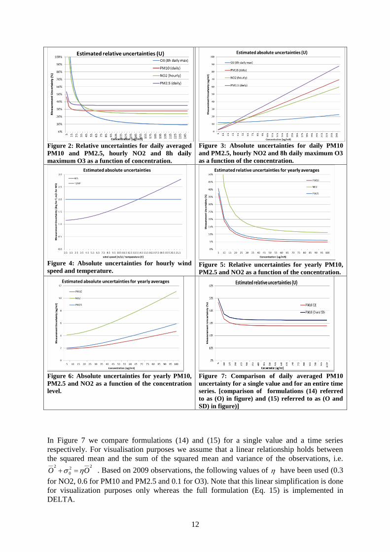
TEMP (test) 2.00 0.025 25 K 1.000 NA NA Table 5: List of the parameters used to calculate the uncertainty (see formulas (15) and (16))

The values reported in this table can be used to produce uncertainty curves for each

compound (see figures below). Parameters for other species than those mentioned in the

above table can be implemented easily in DELTA (see next Concepts Section 6.1 for more

details)

12

Figure 2: Relative uncertainties for daily averaged

PM10 and PM2.5, hourly NO2 and 8h daily

maximum O3 as a function of concentration.

Figure 3: Absolute uncertainties for daily PM10

and PM2.5, hourly NO2 and 8h daily maximum O3

as a function of the concentration.

Figure 4: Absolute uncertainties for hourly wind

speed and temperature.

Figure 5: Relative uncertainties for yearly PM10,

PM2.5 and NO2 as a function of the concentration.

Figure 6: Absolute uncertainties for yearly PM10,

PM2.5 and NO2 as a function of the concentration

level.

Figure 7: Comparison of daily averaged PM10

uncertainty for a single value and for an entire time

series. [comparison of formulations (14) referred

to as (O) in figure) and (15) referred to as (O and

SD) in figure)]

In Figure 7 we compare formulations (14) and (15) for a single value and a time series

respectively. For visualisation purposes we assume that a linear relationship holds between

the squared mean and the sum of the squared mean and variance of the observations, i.e.

22

0

2

OO . Based on 2009 observations, the following values of have been used (0.3

for NO2, 0.6 for PM10 and PM2.5 and 0.1 for O3). Note that this linear simplification is done

for visualization purposes only whereas the full formulation (Eq. 15) is implemented in

DELTA.

13

4.5. An alternative formulation for the observation uncertainty

The uncertainty formulation (14) requires two parameters to be defined: the proportionality

coefficient and the relative expanded uncertainty RV

rkuRV

rU , around an arbitrarily fixed

reference concentration (RV). Because the first of these two parameters is not always

straightforward to establish, we propose here an alternative formulation.

Equation (14) can be re-written as a linear relationship between the squared uncertainty (U2)

and the squared concentration (O2):

2

2

22222 )1()1( ORV

UURVOUU

RVRVRV

r

But this linear relationship can also be simply expressed as:

2

22

2222 O

LRV

UUUU

LRVL

where L is a low range concentration value (i..e close to zero) and UL its associated absolute

expanded uncertainty. Comparing the two formulations we get:

(18) 1

(17)

22

2

22

2

LRVRV

UUU

U

U

RVRVL

RV

L

The two above relations (17) and (18) allow switching easily from one formulation to the

other. The first formulation requires defining values for both and RV

rkuRV

rU , around an

arbitrarily fixed reference value (RV), while the second formulation requires defining

uncertainties around two arbitrarily fixed concentrations (RV and L). An equivalent to Table

5 for the second methodology is provided below with L=0.

RV Np Nnp

NO2 200 ug/m3 48 ug/m3 9.6 ug/m3 5.2 5.5

O3 120 ug/m3 15.1 ug/m3 11.9 ug/m3 NA NA

PM10 50 ug/m3 14 ug/m3 1.87 ug/m3 40 1

PM25 25 ug/m3 9 ug/m3 2.01 ug/m3 40 1

WS (test) 5 m/s 1.3 m/s 1.16 m/s NA NA

TEMP (test) 25 K 1.25 K 1.25 K NA NA

A practical example of introduction of the uncertainty parameters using the second

methodology is provided in User‟s Guide section 6.1

4.6. The 90% principle

For all statistical indicators used in DELTA for benchmarking purposes the approach

currently used in the AQD has been followed. This means that the model quality objective

14

must be fulfilled for at least 90% of the available stations. Given the integer nature of the

station number this criteria sometimes means a larger than 90% of the available stations to

fulfil the criteria. For example all stations will need to fulfil the criteria if the number of

stations is lower than 10. This point is also relevant when considering group of stations (see

User‟s Guide Section 5.1) when the 90% option is selected; the number of stations which can

be discarded and the effective percentage of stations kept within a given group depends on

the number of stations composing this group.

5. Benchmarking report

These reports are currently available for the hourly NO2, the 8h daily maximum O3 and daily

PM10 and PM2.5.

5.1. Hourly frequency

Target Diagram (Fig9 Upper diagram)

The MQO as described by Equation (1) is used as main indicator. In the normalised Target

diagram, it represents the distance between the origin and a given station point. As mentioned

above the performance criterion for the target indicator is set to unity (circle limit) regardless

of spatial scale and pollutant and it is expected to be fulfilled by at least 90% of the

available stations. The normalised bias (first term on the right hand side of Equation [3]) is

use for the vertical axis while the centred root mean square error (CRMSE) (sum of the two

last terms on the right hand side of Equation [3]) ius used to define the X axis.

The percentage of stations fulfilling the target criterion is indicated in the upper left corner

and is meant to be used as the main indicator in the benchmarking procedure. As mentioned

above, values higher than 90% must be reached. The uncertainty parameters ( RV and ,,RV

rU

) used to produce the diagram are listed on the top right-hand side.

The four quadrants in the Target diagram correspond to the following conditions, all based on

Equation (3):

Condition I Condition II Position in target

diagram

2

R-1σ2σ

2

σσ

22

MO

2

2

OM

2

2

UUU RMSRMSRMS

NMB

0NMB Top quadrant

2

R-1σ2σ

2

σσ

22

MO

2

2

OM

2

2

UUU RMSRMSRMS

NMB

0NMB

Bottom quadrant

2

2

2

MO

2

2

OM

2

2

R-1σ2σ

2

σσ

UUU RMS

NMB

RMSRMS

2

MO

2

2

OM

2

R-1σ2σ

2

σσ

UU RMSRMS

Right quadrant

2

2

2

MO

2

2

OM

2

2

R-1σ2σ

2

σσ

UUU RMS

NMB

RMSRMS

2

MO

2

2

OM

2

R-1σ2σ

2

σσ

UU RMSRMS

Left quadrant

The equation used to distinguish the right (SD) from the left quadrants (R) (condition II) can

be rewritten as:

15

)1(2

1σ

R-12σ

σ

σσ

2

R-1σ2σ

2

σσ 2

O

M

2

o

2

OM

2

MO

2

2

OM

NMSD

NMSDR

RMSRMS UU

Or in graphical terms:

Figure 8: Split between R- and SD-dominated errors in the Target diagram. (R,SD) indices couples falling

in the blue shaded area will be located on the left quadrant, others on the right quadrant.

It is straightforward from this diagram to identify which couples of SD and R indices will

lead the station to be within the left or right quadrants

In addition the Target diagram also allows distinguishing easily the performances for single

stations or group of stations (e.g. different geographical regions in this example) by the use of

different symbols and/or colours.

More details on this adapted Target diagram can be found in METHOD2012.

Summary Report (Fig.9 Lower diagram)

The summary statistics table provides information on model performances. It is meant as a

complementary source of information to the MQO (upper diagram) to identify model

strengths and weaknesses. The summary report is structured as follows:

o ROWS 1-2 (OBS) provide the measured observed means and number of exceedances for

the selected stations. In benchmarking mode, the threshold values for calculating the

exceedances are set automatically to 50, 120 and 200 for the daily PM10, the hourly NO2

and the 8h daily O3 maximum, respectively. For other variables (PM25, WS…) for which

no threshold exists, the value is set to 1000 so that no exceedance will be shown.

o ROWS 3-6 (TIME) provide an overview of the temporal statistics for bias, correlation

and standard deviation as well as information on the ability of the model to capture the

highest range of concentration values. Each point represents a specific station. Values for

these four parameters are estimated via equations (7), (8), (9) and (13) respectively. The

green shaded area represents criteria fulfilment. The orange shaded area (for the three first

16

indicators) represents fulfilment but the error associated to the particular statistical

indicator is dominant (see Concepts Section 4.2 and Table 4 in particular for more

details). Note again that fulfilment of the bias, correlation, standard deviation and

high percentile related indicators does not guarantee that the overall MQO based on

RMSE is fulfilled. o ROWS 7-8 (SPACE) provide an overview of spatial statistics for correlation and standard

deviation. Average values over the selected time period are first calculated for each

station and these values are then used to compute the spatial correlation and standard

deviation. Fulfilment of the performance criteria (8) and (9) is then checked for these

values. As a result only one point representing the spatial correlation of all selected

stations is plotted. Colour shading follows the same rules as for rows 3-5.

Note that for indicators in rows 3 to 8, values beyond the proposed scale will be represented

by the station symbol being plotted in the middle of the dashed zone on the right/left side of

the proposed scale

For all indicators, the third column provides information on the number of stations fulfilling

the performance criteria (green beyond 90% of the stations fulfilling, red below 90%).

17

Figure 9: Example of benchmarking performance summary report

18

5.2. Yearly frequency

Scatter Diagram (Fig.10 Upper diagram)

The MQO described in Concepts Section 4.1 for yearly averaged results (i.e. based on the

bias) is used as main indicator. In the scatter plot, it is used to represent the distance from the

1:1 line. As mentioned above it is expected to be fulfilled by at least 90% of the available

stations. The uncertainty parameters ( npp N and N RV, ,,RV

rU ) used to produce the diagram

are listed on the top right-hand side

The Scatter diagram also provides information on performances for single stations or group

of stations (e.g. different geographical regions in this example below) by the use of symbols

and colours.

More details on the scatter diagram and possible options can be found in METHOD2012.

Summary Report (Fig.10 Lower diagram)

The summary statistics table provides information on model performances. It is meant as a

complementary source of information to the bias-based MQO to identify model strengths

and weaknesses. It is structured as follows:

o ROW 1 (OBS) provides the measured observed means for the selected stations.

o ROW 2 (TIME) provides information on the fulfilment of the bias-based MQO for each

selected stations. Note that this information is redundant with the scatter diagram but kept

if the summary report is used independently from the scatter diagram.

o ROWS 3-4 (SPACE) provide an overview of spatial statistics for correlation and standard

deviation. Annual values are used to calculate the spatial correlation and standard

deviation. Criteria (8) and (9) are here used to check fulfilment of the performance

criteria. The same explanation for the green and orange shaded areas as for the hourly

report holds.

Note that for indicators in rows 2 to 4, values beyond the proposed scale will be represented

by the station symbol being plotted in the middle of the dashed zone on the right/left side of

the proposed scale

The third column provides information on the number of stations fulfilling the performance

criteria, Green beyond 90% of the stations fulfilling and red below.

19

Figure 10: Example of benchmarking performance summary report

20

6. References

Cuvelier C., P. Thunis, R. Vautard, M. Amann, B. Bessagnet, M. Bedogni, R. Berkowicz, J. Brandt,

F. Brocheton, P. Builtjes, C. Carnavale, A. Coppalle, B. Denby, J. Douros, A. Graf, O. Hellmuth, A.

Hodzic, C. Honoré, J. Jonson, A. Kerschbaumer, et al., 2007: CityDelta: A model intercomparison

study to explore the impact of emission reductions in European cities in 2010. Atmospheric

Environment, Volume 41, Issue 1, Pages 189-207

Thunis P., L. Rouil, C. Cuvelier, R. Stern, A. Kerschbaumer, B. Bessagnet, M. Schaap, P. Builtjes, L.

Tarrason, J. Douros, N. Moussiopoulos, G. Pirovano, M. Bedogni, 2007, Analysis of model responses

to emission-reduction scenarios within the CityDelta project, Atmospheric Environment, Volume 41,

Issue 1, January 2007, Pages 208-220

Thunis P., E. Georgieva, S. Galmarini, 2010: A procedure for air quality models benchmarking.

(http://fairmode.ew.eea.europa.eu/fol568175/work-groups)

P. Thunis, A. Pederzoli, D. Pernigotti, 2010: Performance criteria to evaluate air quality modeling

applications, Atmospheric Environment, Volume 59, November 2012, Pages 476-482

Thunis P., D. Pernigotti and M. Gerboles, 2012: Model quality objectives based on measurement

uncertainty: Part 1: Ozone. 2012 Atmospheric Environment, Volume 79, November 2013, Pages 861-

868

Pernigotti D., P. Thunis, M. Gerboles and C. Belis.2012. Model quality objectives based on

measurement uncertainty: Part II: PM10 and NO2. Atmospheric Environment, Volume 79, November

2013, Pages 869-878

21

Part II

User’s Guide

22

1. What’s new

1.1. From version 5.0 to 5.1

All benchmarking summary performance report are now produced in jpg format (in place of

postscript previously)

Fonts are optimized for (1) better display and (2) compatibility with Linux operating systems

A correction to the implementation of formula (8) [MQO correlation] has been made

1.2. From version 4.0 to 5.0

An installer is now provided for DELTA under Windows environment. No prior installation of

the IDL virtual machine is any more requested. A demo dataset is provided within this

installer. See installation instruction in the next section.

A Linux version is available for download. See installation instruction in the next section.

The utility function “Data-Check Integrity Tool” is automatically run by default with new

datasets to check the consistency of the input data files. This run is performed once only.

Note that at first application, this function will also convert automatically the observation

data from csv to cdf format to speed-up future use with DELTA.

Modelling data entered in “csv” format can be converted to “cdf” format through a

convertion functionality incorporated in the DELTA tool (old csv2cdf).

Percentiles value for O3 and PM10/PM2.5 used to calculate the high percentile indicator

included in the summary report have been set to correct values (from 90.4 to 92.9% for O3

and from 93.1 to 90.1% for PM2.5 and PM10). Values have been corrected in the first part of

this guide accordingly.

Paths to existing applications (Word, Excel, Google Earth…) need to be set in the init.ini file

in the resource directory. This operation can now be done automatically through the “Find

external application paths” in the help menu. Note that this operation requires a substantial

amount of time but will be performed once only.

Some minor bugs in the formula of Tables 2, 3 and 4 in the first Section have been corrected.

For yearly models:

o The mouse recognize functionality has been re-activated for the summary report

(bug fix)

o Monitoring data can be formatted in one single “csv” file

1.3. From version 3.4 to 4.0

Inclusion of a new diagram “geomap” for hourly/daily model results.

The X-axis of the target diagram is positive in both directions.

Uncertainty parameters are now indicated on the target diagram and on the scatter

diagram

Addition of new MQO for PM2.5, WS and TEMP. Parameters for the PM2.5 MQO

have been revised to avoid uncertainties smaller than PM10 in the lower

concentrations range.

23

Update of uncertainty parameters for NO2 and PM10 (yearly and hourly)

Inclusion of the myDeltaInput option to facilitate the management of multiple

datasets. Note that DELTA can run in absence of this new input file.

Inclusion of MQO for SO4, NH4, NO3, EC and TOM for testing purposes.

Uncertainty parameters are available in the “goalscriteria_oc.dat” configuration file.

Correction of geomap SD and R error symbol types: switch to be consistent with

Target.

Correction of the counting of valid station in the yearly scatter diagram

Modifications of the hourly/daily summary report: the RDE indicator has been

suppressed and substituted by a threshold indicator

The bug in the summary report (calculation of the spatial correlation and spatial

standard deviation – no point appearing) has been fixed.

The legend of the summary report has been re-designed

Modification of the yearly summary report: RDE has been dropped.

Correction of Target diagram: SD and R related errors were assigned the wrong side

of the diagram (left vs. right)

Uncertainty values for PM10 TEOM and beta-ray measurement techniques have been

included in the “goalsandcriteria_oc” configuration file. See here for more details.

Addition of a “save main statistical indices” option. This option runs automatically

when the summary report diagram is selected. See here for more details.

Correction: The generation of performance reports in pdf format did not work

properly in version 3.6.

The MQO for 3h average NO2 has been removed

2. Installation and running steps

The current version of the Delta Tool is available for Windows and Linux environments.

Installation and running steps under WINDOWS

Download and run the setup.exe file available on the Delta web page. This will create

a “Delta Tool” icon on the desktop as well a “JRC_DELTA” menu in the Windows

start menu (lower left icon on your desktop). You can launch the application by

double-clicking on the icon.

After the first installation the software is configured to operate with a demo dataset. If

you wish to re-use data you produced with an earlier version of the software, please

follow the below steps:

o Access the $home$ directory through the JRC_DELTA menu.

o Create a sub-directory under data/monitoring, e.g. “Mydata” (parallel to demo)

and include in it your monitoring data.

o Create a sub-directory under data/modeling, e.g. “Mydata” (parallel to demo)

and include in it your modeling data

o Include your startup.ini file and rename it into startup_MyData.ini in the

resource sub-directory

24

o Adapt the names and paths in the MyDeltaInput file (change demo into

Mydata). The MyDeltaInput is placed on the resource subdirectory but is also

accessible through the start menu.

o Re-start the Delta application

A “JRC-DELTA” program item in the start menu gives you access to 1) the home

installation directory, 2) the MyDeltaInput configuration file, 3) the user‟s guide and

4) the web-site.

Installation and running steps under LINUX

Download and uncompress the setup_linux.tar.gz file available on the Delta web page

in a new directory (e.g. DeltaTool). This will create a DeltaTool.exe as well as a sub-

directory structure (resource, configuration, data...). You will need to do the following

operations:

1) Edit the “app.folder.ini file and modify the absolute path (e.g.

/home/…/DeltaToolV51/). Do not forget the final “/” at path end.

2) Allow execution permission to the file DeltaTool (chmod +x deltaTool)

3) If permission error persist, change all permission of folders and subfolders to

allow execution mode (chmod -R 777)

You can then launch the application by running the DeltaTool executable

(./DeltaTool). Note that some screen applications (e.g. putty) generate problems.

After the first installation the software is configured to operate with a demo dataset. If

you wish to re-use data you produced with an earlier version of the software, please

follow the below steps:

o Create a sub-directory under data/monitoring, e.g. “Mydata” (parallel to demo)

and include in it your monitoring data.

o Create a sub-directory under data/modeling, e.g. “Mydata” (parallel to demo)

and include in it your modeling data

o Include your startup.ini file and rename it into startup_MyData.ini in the

resource sub-directory

o Adapt the names and paths in the MyDeltaInput file (change demo into

Mydata). The MyDeltaInput is placed in the resource subdirectory.

o Re-start the Delta application

o Paths will need to be updated in the init.ini file (under the resource sub-

directory) to allow some external applications to run (Word, pdf reader…).

The user‟s guide is available in the help sub-directory

3. Preparation of input files

In order to run the Tool, the following files have to be prepared by the user

The configuration file <startup.ini>. This file is located in folder ...\resource. For

handling different data (obs – mod) sets, see Users Guide Section 6.4

Files with observed data (one file for each monitoring station). These files should be

in ”csv” or “cdf” format and be placed in folder ...\data\monitoring

25

Files with modeled data at the locations of the stations (one file per model and

scenario). Such files should be in “csv” or “cdf” format. If only “csv” files are

available, DELTA will automatically create a “cdf” version at first use. Each .cdf file

may contain model results for several locations (stations). The .cdf files should be

placed in folder ...\data\modeling. If results from more than one model are used, the

utility to create cdf files from csv files should be used (available from help menu, see

Section 9.2).

The file “MyDeltaInput” in the resource directory should then be adapted to the paths

and file names selected by the user.

3.1. Init.ini

The resource folder contains an ASCII file named init.ini where specific software (WORD,

ADOBE...) location information should be provided. The user should modify the paths

according to his personal installation settings. This is needed, e.g, to be able to use the help in

the Delta Tool. The right hand side of the following lines (end of the init.ini file) should be

adapted. This updating operation can be done manually or automatically through the help

menu (“find external application paths”). Note that this operation might require a

substantial amount of time but will be performed once only on a given computer.

BROWSER_LOCATION=C:\Program Files\Mozilla Firefox\firefox.exe

WORKSHEET_LOCATION=C:\Program Files\Microsoft Office\OFFICE11\EXCEL.EXE

DOCUMENTSREADER_LOCATION=C:\Program Files\Microsoft Office\OFFICE11\WINWORD.EXE

NOTEPAD_LOCATION=notepad.exe

PDFREADER_LOCATION=C:\Program Files\Adobe\Acrobat 7.0\Acrobat\Acrobat.exe

GOOGLEEARTH_LOCATION=C:\Program Files\Google\Google Earth\client\googleearth.exe

3.2. Startup.ini

The configuration file (startup.ini) is common to both inputs with hourly and yearly

frequencies. It is located in ...\resource. The file is in ASCII format and contains some

general information about the spatial scale, the parameters selected for evaluation and the

characteristics of the monitoring stations. The file has three main sections:

MODEL – includes information about the year, spatial scale and input frequency.

PARAMETERS - includes variable names and measurement units

MONITORING – includes list of all stations with their siting characteristics and

parameters measured.

The following conventions apply:

Each blank row or each line beginning with "[", ";" or "#" will be discarded

No blanks between fields are permitted

Line breaks are not allowed.

The three section headers: “[MODEL]”, “[PARAMETERS]” and “[MONITORING]”

are compulsory,

Station codes and abbreviation codes must be unique.

The station names should not include blanks and special characters such as “.”,” ‟ ”,

“;”,”-“

26

Only the symbol “_” is allowed.

Variables must be separated by an asterisk.

The station names must be EXACTLY (including case sensitivity) the same used in

the observation data files and modeled data files.

Example:

[MODEL]

;Year

;frequency

;Scale

2009 hour

urban

[PARAMETERS]

;Species;type;measure unit

SO2;POL;gm-3

NO2;POL; gm-3

PM25;POL; gm-3

PM10;POL; gm-3

WS;MET; m/s

TEMP;MET; C

[MONITORING] Stat_Code;Stat_Name;Stat_Abbreviation;Altitude;Lon;Lat;GMTlag;Region;Stat_Type;Area_Type;Siting; listOfvariables

IT00000;station0;STAT0;681.;8.931;44.31;GMT+1;Lombardia;Background;Urban;Plane;TEMP*PM10*O3;

IT00001;station1;STAT1;962.;10.03;44.97;GMT+1;Veneto;Traffic;SubUrban;Hilly;TEMP*O3;

IT00002;station2;STAT2;851.;11.34;44.18;GMT+1;Piemonte;traffic;urban;Mountain;WS*PM10*O3*SO2;

IT00003;station3;STAT3;806.;7.597;46.02;GMT+1;Emilia-Romagna;Industrial;Rural;Valley;WS;

IT00004;station4;STAT4;769.;8.222;44.29;GMT+1;Lombardia;Background;Urban;Plane;TEMP*O3;

IT00005;station5;STAT5;163.;9.193;45.85;GMT+1;Friuli Venezia Giulia;Unknown;Unknown;Coastal;PM10;

...

<EOF>

Description:

[MODEL] section:

The first three lines are just comments

Year: year of interest

Frequency (lowercase): Either hour or year. This parameter should be set to “hour”

for models delivering outputs with an hourly or daily frequency and set to “year‟ for

models delivering outputs as annual averages (see User‟s Guide Section 3.5).

Scale (lowercase): Either local (traffic), urban or regional. But not used currently

[PARAMETERS] section:

The first line is a comment which gives a hint of the contents of the following lines:

Species: name of the variable (lower or upper case but should be consistent with

observation and modeling files)

Type: “POL” and “MET” indicate air quality and meteorological variables

respectively. These categories are created to facilitate filtering during the selection

phase and can be defined by the user at his convenience.

27

Measure units: the units MUST be μgm-3 for concentrations. For the other variables,

see the notes below.

Notes:

Each line contains the name of a parameter, the type and the measurement unit,

separated by semicolons. The parameters are those available in the observation

dataset. It is permitted to have lines with parameters not present in the dataset. The

sequence of parameters is irrelevant.

Some parameter names and units are pre-assigned and should be obligatory followed

(since they are used in the benchmarking procedure): O3 [μgm-3], NO2 [μgm-3],

PM10 [μgm-3], WS [ms-1] (wind speed), TEMP [degC] - temperature, SH [g/kg]

(specific humidity)

[MONITORING] section

The first row contains the labels. The labels currently referred to as: region, station type, area

type and siting can be modified by the user and will appear as modified in the data selection

window. Each subsequent row refers to a given station, where:

Stat_Code: national identification of the station e.g. AT0001ST, or VEN00356, or

user‟s assigned code (e.g. STAT001)

Stat_Name (case sensitive): combination of letters and/or numbers ; only the symbol

“_” is allowed blanks and special characters are not allowed

Stat_Abbreviation: station name abbreviation (4 letters). The abbreviation will be the

one identifying the station on the DELTA output graphs and statistics

Altitude: height above sea level (in meters)

Lon, Lat: Longitude and Latitude (in decimal degrees)

GMTlag: Time zone (currently not used)

Region: Name of the administrative region to which the station belongs. In alternative

– a user defined region (Naming rules similar to “Stat_Name”)

Stat_Type: background, traffic, industrial

Area_Type: urban, suburban, rural

Siting: Categories are proposed: mountain, hilly, plane, valley or coastal. They will be

used eventually to group stations and calculate average statistics for each group; If

other categories suit better user‟s stations, they can be defined here.

listOfvariables..: The variables measured at each station , (PM10, O3, WS etc). The

variables are separated by an asterisk.

Note: It is left to the user to assign appropriate fields to classify stations. In our example,

REGION, STAT_type, Area_Type and Siting are selected but other choices could have

been made. These choices will configure the widget menus to help with the selection of

stations according to the chosen fields.

28

3.3. Observation file

3.3.1. Hourly Frequency

Monitoring stations to be used with the Tool may have either air quality data, either

meteorological data or both.

csv format

Files names and type:

Each station must have an associated file containing the data in comma separated

format and with extension .csv, e.g. “station1.csv”

The file names should be consistent (including case sensitivity) with the naming rules

used in the configuration file (startup.ini).

Files location:

….\data\monitoring

Files structure:

The first row must contain the labels of the columns: year (4 digits), month (1-12), hour

(0-23) and the names of the observed parameters at each station. Following lines should

include the observed values on an hourly basis (8760 rows (or 8784 for leap year) if entire

year is available). If for a given hour data are missing for all parameters, the line can be

omitted. Data are recognized by their associated date and time.

Example: filename <station1.csv>

year;month;day;hour;O3;PM10;WS;WD;TEMP;

2005;1;1;0;40.1;55.4;0.75;310;15.6;

2005;1;1;1; 40.1;55.4;0.75;310;15.6;

2005;1;1;2; 40.1;55.4;0.75;310;15.6;

…

2005;12;31;23; 40.1;55.4;0.75;310;15.6;

<EOF>

Particular requirements:

The station names used in startup.ini must be used for each one of these files.

For non-annual average values each file must contain observation values on an hourly

basis. For leap years, data for February 29th

may be included in the files.

Data will be read by dates. Missing dates (i.e. lines) will automatically be treated by

DELTA as -999.

If data are monitored on a daily basis (e.g PM10), please put the daily value at all

hours from 0 to 23 for this day.

29

Remark: Daily deposition observations (for example rain) should be distributed over the

24 hours of the particular day.

If both air quality and meteorological measurements are available for the same site,

the data must be included in the same file (as in the example above)

Each blank row or beginning with "[", ";" or "#" will be discarded

Spaces are not permitted between the fields.

Line breaks are not allowed.

The semi-column ending each lines is not mandatory

cdf format

The “cdf” format is identical to the one specified for modeling result data (option 2). If

provided as “csv”, the conversion from to “cdf” will be performed automatically when

running DELTA if your set of data is new. If not done automatically, you can always perform

this operation by running the “check integrity tool” available under the help menu.

3.3.2. Yearly Frequency

Option 1: Each station monitoring data is assigned a specific file

Files names and type:

Each station must have an associated file containing the data in comma separated

format and with extension .csv, e.g. “station1.csv”

The file names should be consistent with the naming rules used in the configuration

file <startup.ini> (see Section 3.2).

Files location:

….\data\monitoring

Files structure:

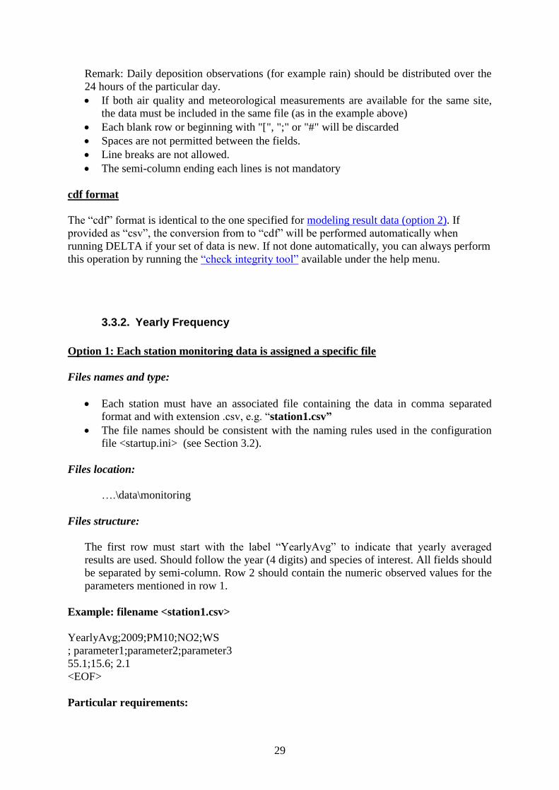
The first row must start with the label “YearlyAvg” to indicate that yearly averaged

results are used. Should follow the year (4 digits) and species of interest. All fields should

be separated by semi-column. Row 2 should contain the numeric observed values for the

parameters mentioned in row 1.

Example: filename <station1.csv>

YearlyAvg;2009;PM10;NO2;WS

; parameter1;parameter2;parameter3

55.1;15.6; 2.1

<EOF>

Particular requirements:

30

The station names used in startup.ini must be used for each one of these files.

If data are missing the gaps should be filled by -999.

If both air quality and meteorological measurements are available for the same site,

the data must be included in the same file (as in the example above)

Each blank row or beginning with "[", ";" or "#" will be discarded

Spaces are not permitted between the fields.

Line breaks are not allowed.

Option 2: All station monitoring data are assigned to a single file

This “csv” format should be identical to the one specified for yearly modeling result data.

Important: the name of the file is mandatory: “OBS_Yearly.csv”

3.4. Model file

3.4.1. Hourly Frequency

Modeled data can be prepared in one of the following formats:

netcdf (option 1) format (one single file for a given model and time period. A ncdf-

variable must be generated for each station/species combination

netcdf (option 2) format (one single file for a given model and time period. A ncdf-

variable must be generated for each station.

csv format (similar to the one described for the observations). Such files can then be

converted to “cdf” format through the conversion utility functionality available under

the help menu.

Description of the netcdf (option 1) format

One single netcdf file should be provided for a given model. It must contain a time

series for each station and variable listed in <startup.ini >.

The names of the parameters should be the same as in the configuration file

<startup.ini>.

The units in the netcdf file should be the same as specified in startup.ini

Files location:

….\data\modeling

Files structure:

31

Each data block inside the netCDF file should be named as “StatName_Parameter” (see

examples below) where “StatName” is the name of the station corresponding to the one set

in the <startup.ini >, and “Parameter” refers to the modeled pollutants and meteorological

variables, as indicated in the <startup.ini >

Each data block should contain either (a) 1 year of hourly data for each station and parameter

(1dimensional array with 8760 [8784 for leap years] hourly data) or (b) a specific time period

smaller than the entire year. In the latter case an additional attribute should be included in the

netCDF file to set the initial starting time (in hours) as follows (global attributes: StartHour =

1320 indicating that the period of interest starts at hour=1320). Within the specific time

period data should be continuous, i.e. include missing values as “-999”.

In the case of a leap year model results for February 29th should be included (or set to -999)

if the period contains this day.

Modeled data at a given station may contain either air quality fields, meteorological fields or

both.

Example: <2008_WRFCHIM_TIME.cdf>

netcdf 2008_WRFCHIM_TIME.cdf {

dimensions:

T = 8760 ;

variables:

float station0_CO2(T);

float station1_NO2(T);

float station1_WS(T);

float station1_WD(T);

float station2_CO2(T);

float station2_NO2(T);

float station2_WS(T);

float station2_WD(T);

}

Example: <2008_WRFCHIM_TIME.cdf> with time period less than entire year

netcdf 2008_WRFCHIM_TIME.cdf {

dimensions:

T = 744 ;

global attributes: StartHour = 1320s ; variables: float station0_CO2(T);

float station1_NO2(T);

float station1_WS(T);

float station1_WD(T);

float station2_CO2(T);

float station2_NO2(T);

float station2_WS(T);

float station2_WD(T);

}

Particular requirements: If a parameter is entirely missing (i.e. not provided by the model)

for a station, but the same parameter is present in the monitoring dataset for the same station,

the user must include that parameter in the *.cdf file as an hourly series of “-999”.

32

Description of the netcdf (option 2) format

One single netcdf file should be provided for a given model. For each station it must

contain a time series for each variable listed in the <startup.ini> file.

All parameters (i.e. variables, e.g. NO2, PM10...) should be defined in byte format in

a systematic order defined in a global attribute.

The names of the parameters should be the same as in the configuration file

<startup.ini> (see Section 2.2).

Files location:

….\data\modeling

Files structure:

Each data block inside the netCDF file should be named as “StatName_Parameter” (see

examples below) where “StatName” is the name of the station corresponding to the one set

in the <startup.ini >

Each data block should contain either (a) 1 year of hourly data for each station and parameter

(2 dimensional array with 8760 [or 8784 for leap years] hourly data). Or (b) a specific time

period smaller than the entire year. In the latter case an additional attribute should be included

in the netCDF file to set the initial starting time (in hours) as follows (global attributes: StartHour = 1320 indicating that the period of interest starts at hour=1320). Within the specific time period data should be continuous, i.e. include missing values as “-999”.

Modelled data at a given station may contain either air quality fields, meteorological fields or

both.

Example: <2008_CHIM_TIME.cdf>

netcdf 2008_CHIM_TIME.cdf {

dimensions:

V = 3 ;

T = 8760 ;

variables:

float station0 (T,V);

float station1 (T,V);

float station2 (T,V);

// global attributes :

: Parameters = 78b, 79b, 50b, 32b, 80b, 77b, 49b, 48b, 32b, 79b, 51b ;

}

Here ‘78b, 79b, 50b, 32b, 80b, 77b, 49b, 48b, 32b, 79b, 51b’ is the byte

format of ‘NO2 PM10 O3’.

Example: <2008_CHIM_TIME.cdf> with given time period (less than entire year)

netcdf 2008_CHIM_TIME.cdf {

dimensions:

V = 3 ;

T = 744 ;

33

global attributes: StartHour = 1320s ; variables:

float station0 (T,V);

float station1 (T,V);

float station2 (T,V);

// global attributes :

: Parameters = 78b, 79b, 50b, 32b, 80b, 77b, 49b, 48b, 32b, 79b, 51b ;

}

Here ‘78b, 79b, 50b, 32b, 80b, 77b, 49b, 48b, 32b, 79b, 51b’ is the byte

format of ‘NO2 PM10 O3’.

Particular requirements: If a parameter is entirely missing (i.e. not provided by the model)

for a station, but the same parameter is present in the monitoring dataset for the same station,

the user must include that parameter in the *.cdf file as an hourly series of “-999”.

3.4.2. Yearly Frequency

Modeled data should be prepared in ASCII (csv) format. One single file should be provided

for a given model. It must contain annual average values for each station listed in

<startup.ini>.

File name: <YEAR_MODELNAME_TIME.csv>

Files location: .\data\modeling

Files structure:

YearlyAvg;2009;O3;PM10...

;Station;ValueParam1;ValueParam2...

Illmitz;40.3;45.34

Pillers;78;54.54

...

3.5. Using DELTA with yearly output

By default the input files are configured for hourly frequency models but for models

delivering annual averages it is possible to tune all configuration files to keep only relevant

diagrams and elaborations within the selection menus (e.g. all diagrams using correlation will

be discarded). For doing this, go in your startup.ini file and set the frequency parameter to

“year”.

4. Delta Tool top menu

34

When starting Delta Tool the upper right-hand corner contains a menu that allows you, e.g. to

run a Benchmark, and to save and retrieve selections you have made.

File

o Save image: Save main window diagram in various format (jpeg, tif...).

Images are saved in the subdirectory “save”

o Exit

Benchmark (see Section 4)

o Assessment

daily 8h maximum O3

Daily averaged PM10

Daily averaged PM25

Hourly NO2

Yearly PM10

Yearly NO2

o Planning (not available yet)

Mode

o Select mode (inactive)

o Hide/Show Recognize Info: Mouse recognize window is turned on/off

Data selection

o Select data: Opens the “Data selection” window (similar to “data selection”).

o Save data: Save current “data selection”

o Restore data: Restore “data selection” from existing ones.

Analysis

o Select Analysis: Opens the “Analysis” window (similar to “Analysis”).

o Save Analysis: Save current analysis choices.

o Restore Analysis: Restore “analysis” from existing ones

Help

o Help file: Open the current DELTA version User‟s guide (pdf format). The

correct directory in which “acrobat.exe” is located should be specified in the

“init.ini” file in the “resource” directory (but this can be performed

automatically – see option below).

o Data check Integrity Tool: Open an independent window with the Check-IO

processor to check consistency of the input data (see User‟s Guide Section

9.1)

35

o Delta WWW: Open the DELTA WWW homepage. The correct directory in

which the browser executable is located should be specified in the “init.ini”

file in the “resource” directory.

o About: Version information

o Find external application paths: Automatically update the paths to external

applications (Word, Excel…). This operation might require a substantial

amount of time but only needs to be performed once.

o Licence: End user licence agreement

5. Exploration mode

In order to calculate a given statistical indicator and visualize it by a diagram the user has

first to make selections in two interface windows – “data selection” and “analysis window”

(activated through the starting window, see User‟s Guide Section 5). The data selection and

analysis interfaces are described in User‟s Guide Sections 5.1 and 5.2 respectively. Finally

the main DELTA graphical interface, which reflects the options previously selected by the

user in the two interface windows, is described in User‟s Guide Section 5.3.

Figure 11 The DELTA main interface (starting window)

5.1. The data selection interface

36

A selection has to be made by the user in terms of

o a model/scenario (year) pair

o a parameter (e.g. NO2)

o a monitoring station

An example is given in Figure 12.

In brief, the selections are made in the following way:

Model selection: In the left pane select one or more models + scenarios.

Parameter selection: In the right pane first select Type, then Parameters (you may

select several elements by Ctrl + Click).

Station selection: The panels Region, Station Type, Area Type and Siting indicate

some filters, which may help you in selection of stations. Apply relevant filters, so the

panel Available becomes populated with some stations. Use Ctrl + Click on those you

wish to select. Finally, click the Add button to make the selection effective.

Optionally save: You may save the list of stations by clicking the ‟Save Obs‟ button

(the „Load Obs‟ button allows you to retrieve a previously saved list).

Some more details follow.

Various filters are available to facilitate the selection of the appropriate monitoring stations in

terms of regions, types. These filters are defined in the configuration file <startup.ini>, where

the user can make the station classification categories case specific.

Note: When a user selects a parameter (e.g. O3) in the "data selection" window, all stations

measuring that parameter automatically appear in the "available" section. The user can then

make his selection among these available stations and add them in the “selected” section. At

this stage the user can still change his mind and select another parameter (e.g. PM10). The

list of selected stations will be updated after warning the user.

The user has the possibility to save his choices and to reload them at a later time. Two

modalities exist which can be useful to avoid repeating frequently used selections.

Modality (1): In order to save the selections in the data selection window, choose “save data”

from the top “data selection” pop up menu. A new window appears with the request to put a

file name. File extension must be *.elb. By default the file is saved in the dir…. \save. To

reload the saved selections, -choose “restore data” from the top “data selection” pop up menu.

Modality (2): In order to save the station selection only, press the button „save obs‟ in the

lower right corner of the data selection window. A new window appears with the request to

put a file name. File extension will be *.obl. By default the file is saved in the dir…. \save. To

reload the saved selections, -press the button “Load Obs”.

A set of stations can either be treated as a number of single entities or as a group. In the case

of groups the user will be asked to select between “mean” and “90% percentile” options. In

the first case the mean of the stations statistical indicators will be represented as a single

dot/symbol in the diagram whereas in the second option the worst statistical indicator among

90% of the available stations (rejecting 10%) is selected. This latter choice must be used

37

with diagrams in which performance criteria are present and indicate whether this

criterion is fulfilled for the selected group of stations.

Figure 12: DELTA data selection interface.

5.2. The analysis interface

The analysis interface (Figure 13) allows the user to select the type of statistics and diagram,

as well as the desired temporal operations to be performed on the original data (“Time Avg”

and “Daily Stats”). Available diagrams are described in the Diagram overview Section (Part

III).

Each of these plot types can be selected to illustrate different statistical metrics (statistics

column). This is especially true for the barplots which is the common way to visualise single

statistical metrics (Mean, RMSE, bias, IOA, Exceedance days...). Some of these statistics

require threshold values which can be included (e.g. SOMO, Exceedance days…) on the

same window. The field for threshold values should contain numbers separated by an #.

38

Figure 13: DELTA analysis selection interface

The lower left part of the analysis selection interface (“multiple choice info”) gives

information on the different possibilities offered to the user in terms of combination of

parameters, stations, and models to generate the diagram. These possibilities give the degree

of freedom in selecting items of the four main entities: scenario (year); model; parameter;

monitoring stations. The allowed multiple choices for a given diagram are pre-defined in the

tool and are described in the Diagram overview Section.

On the right side of the analysis selection interface, time operations can be chosen to be

performed on the selected modelled-observed data pairs, i.e.:

Time Avg.: Time series kept as originally formatted (preserve or 1h) or 8h running

average

Daily Stats: Statistical operation applied for each day: mean, max or min.

Season: choice between summer, winter and entire year

Day: Selection between night time hours, daylight hours, entire 24h day, week-ends

and week days.

Note that for some statistics and pollutant choices, these flags will be automatically filled to

the adequate values.

This feature can be useful if you repeatedly use the same set of selections. In order to save the

selections in the analysis window, use the top menu in Delta Tool: click the item “Analysis”

and choose “Save Analysis” in the drop-down menu. A new window appears with the request

to put a file name. File extension must be *.elb. By default the file is saved in the dir…. \save.

To reload the saved selections, click the item “Analysis” on the top menu and choose

“Restore Analysis”.

39

5.3. The main graphical interface

When the user has made his selections in the data selection window and the analysis window

the „Execute‟ tab can be pressed. The Delta Tool‟s main graphical interface will then pop-up

(unless you have made selections that the tool does not support).

The screen is divided into two main areas:

The left side recapitulates the choices made by the user in the previous interfaces which

lead to the generation of a given diagram.

The right side hosts the diagram and accompanying legend (which also summarizes the

options selected by the user). Only one diagram is shown at a time (i.e. no multiple

windows).

Figure 14: DELTA main graphical window.

40

6. DELTA functionalities and user’s tuning options

6.1. “Playing” with uncertainty parameters: the “goals_criteria_oc” input file

In the configuration file “goals_criteria_oc.dat” the user can find lines of the type:

3;PM10;ALL;OU;PMEAN;28*0.018*40*1*50*;Descr of: GC 56

Lines with “OU” as fourth parameter contain all information required to calculate the value

of the observation uncertainty used to derive the model quality objectives for one particular

species and time average. The numbers separated by asterisks can be modified by the user to

test alternative uncertainty estimates. By order, these numbers represent (see equation 16 for

details):

RV

rku (28 in our example) expressed in percentage. This is the expanded

relative uncertainty ( RV

r

RV

r kuU )

(0.018 in our example)

Np and Nnp (40 and 1 in our example)

RL the reference value (50 in our example)

Testing different PM10 measurement uncertainties

Different experimental methodologies exist to measure PM, each characterized by a different

level of uncertainty. The user can test the impact of switching between different uncertainty

estimates, corresponding to values representative of the gravimetric (default reference), beta-

ray and teom techniques. In the “goals_criteria_oc.dat” configuration file, the following lines

are visible:

26;PM10g;ALL;OU;PMEAN;28*0.018*40*1*50

27;PM10t;ALL;OU;PMEAN;38*0.027*40*1*50

28;PM10b;ALL;OU;PMEAN;38*0.009*40*1*50

To switch among the different PM uncertainty estimates it is necessary to copy the number in

between asterisks for the selected uncertainty estimate (PM10g for gravimetric, PM10t for

TEOM and PM10b for beta-ray) and use them in the PM10 line used by DELTA.

Introducing uncertainties for new variables

Two methodologies have been described in Sections 4.4 and 4.5. In the first case the user

knows all required parameters and can introduce a new line at the end of the

“goals_criteria_oc.dat” file as follows:

35;NEWSPEC;ALL;OU;PMEAN;28*0.018*40*1*50*;Descr of: GC 56

The first field is an index number which should increment the index of the previous line by 1.

The second field should contain the name of the new species. Note that the same name should

be kept in all monitoring, modeling and startup files for consistency. The third and fourth

fields should be kept as is (i.e. ALL;OU). The fifth field (PMEAN) is a contraction of the

time average (Preserve, 8H running) and daily stat (Preserve, MEAN, MAX and MIN)

41

options. The fifth field should concatenate the bold identified letters of the two options

according to the choices made. For example O3 8h daily max would lead to “8HMAX” for

the fifth field while daily PM10 would lead to “PMEAN”. The following five fields have

been described above while the last field is a comment to be used at convenience by the user.

In section 4.5 an alternative methodology is described to set these uncertainty parameters. We

provide here an example: assuming that we can estimate that the PM10 uncertainties around 0

and 50 ug/m3 would be 1.88 and 14 ug/m3, respectively. We can calculate easily the

following numbers needed within DELTA.

018.014

88.1

14.0 that implies 2k if which 28.050

14

2

RV

r

RV

r uU

6.2. Saving summary statistics information in ASCII

Delta saves by default all information contained in each diagram in ASCII format by

generating a file named “dumpFile.txt” which can be found in the dump directory. This file

will be overwritten at each new generated diagram

Frequently used statistical indicators (e.g. correlation, bias…) can be automatically created by

selecting the “summary report & print” analysis diagram option. DELTA will then generate

the summary report in the graphical window but also create an ASCII file in the dump

directory using the selected model and species to create the name.

Note that both options will create information relative to the selected time period.

6.3. Mouse-driven recognize functionality

For most graphics a small additional window appears with the title “Info on data points

(click!)”. This allows the user to click on the diagram and retrieve information about the

quantitative values of the different points/stations represented. This feature can be switched

on and off through the top menu in Delta Tool: click the item “Mode” and choose

“Hide/Show Recognizer info”.

6.4. Managing multiple datasets: the “MyDeltaInput” option

As mentioned before there are three different types of input information required to run the

DELTA tool:

The startup.ini file located in the ./resource directory

The YEAR_MODEL_TIME.cdf file located in the ./data/modeling directory

The station.csv files located in the ./data/monitoring directory

When dealing with different statup.ini files, different sets of modelling results, and different

sets of monitoring stations, it may be useful to be able to overwrite the defaults locations of

these three inputs.

42

The file MyDeltaInput.dat in the resource directory contains three lines:

1 - First line contains the name of the startup.ini file in the ./resource directory

2 - Second line contains the location of the model data in the ./data directory

3 - Third line contains the location of the monitoring data in the ./data directory

Example:

startupED2007.ini ; the startup.ini file

modelling_ED2007 ; subdirectory in ,/data

monitoring_ED2007 ; subdirectory in ./data

The default (if the MyDeltaInput.dat file is not found) is: startup.ini

modeling

monitoring

After completion of „Execute‟ the name of the used startup.ini file, the modelling data

location, and the monitoring data location are mentioned beneath the plot.

Note that DELTA can run with/without this new configuration input file.

7. Benchmarking mode

From the Delta Tool top menu select the item “Benchmarking” (this is only possible when

the “Data Selection” window and the “Analysis” window are closed).

At present the automatic production of performance reports is available for the following

pollutant concentrations and time frequencies:

daily maximum 8h mean O3

Daily averaged PM10

Daily averaged PM25

Hourly NO2

Yearly PM10

Yearly NO2

Reports are produced similar to those presented in Section 5 of the “Concepts” part of this

document.

Important:

Currently the performance report is produced automatically for one single model. This single

model is selected by default and corresponds to the top-of-the-list model when opening the

data-selection interface. For applying the procedure to other models the user is requested to

play with the model data files in the ../ data/modeling directory and leave in this directory

only the model on which the performance report should be produced.

43

8. Demo Dataset: Po-Valley

This dataset contains the results from a model inter-comparison exercise performed by two

air quality models for year 2005. The model domain covers the Po Valley (Italy) with at 6 x6

km2 resolution (95x65 cells) grid. Pollutant concentrations have been simulated by 5

transport chemical (CHIMERE, TCAM, CAMX, RCG, MINNI ) of which two are made

available in this demonstration dataset.

Observations from 63 monitoring sites located in the Po Valley are also provided. Sites have

been classified in regions and station types (suburban, urban and rural).

9. Utility programs

9.1. Data-Check Integrity Tool

Aim:

Checking the consistency among the modeling results file (cdf, csv), the observation files

(csv, cdf) and the main configuration file (startup.ini).

Important: The data check integrity step will be performed automatically each time a new

startup.ini is used. If modifications are made in the monitoring or modelling data without

affecting the startup.ini file, please perform this data-check integrity manually to identify

potential consistency issues.

How to use:

From the Delta Tool top menu select the item “Help” > “ Data-Check Integrity Tool” (this

is only possible when the “Data Selection” window and the “Analysis” window are closed).

There are currently 19 steps included in this consistency check:

1) Checking existence of relevant directories

2) Checking existence of “startup.ini” file

3) Checking existence of appropriate sections within startup.ini

4) Checking correctness of “PARAMETERS” section within Startup.ini

5) Checking correctness of “MONITORING” section within Startup.ini

6) Checking for possible redundancy in station names in startup.ini

7) Checking consistency of the number of stations between startup.ini and obs files

8) Checking consistency of the station names between startup.ini and obs files

9) Checking consistency of the species names between startup.ini and obs files

10) Checking number of lines in obs files

11) Conversion of observations files from csv to cdf

12) Checking for extreme values in obs files

13) Checking for zero values (information check only)

14) Checking for existence of model file

15) Checking for correct attribute in model netCdf file

16) Checking correctness of time dimension in model file

17) Checking model extreme values

44

18) Checking consistency between species available in startup.ini and model file

19) Producing statistic report

Check_IO produces a log report, as well as a summary report with details concerning the

various checks. The reports are located in the main directory where Delta Tool is installed.

9.2. Interactive format conversion tool

This tool available under the help menu allows to produce a model file in “cdf” format from

files in csv format similar to the one described for monitoring data. This program works only

for data produced with an hourly frequency. If more than one model is used, this conversion

operation will need to be performed for all models. The user needs to specify the input

directory (where the csv are located), the output directory (where the cdf file will be created)

and the startup.ini file which is used as reference.

Important: User‟s modifications in the widget input lines will only be considered if you type

the “return” key after changes.

9.3. Preproc-CDF

The Deltapreprocessor is an idl-based tool for the extraction of time series at observational

locations from meteorological or air quality model output for use in the DELTA Tool. Input

to the PreProcessor is the configuration file 'startup.ini' containing the variables

(meteorological variables , and pollutants) to be treated, as well as geographical information

about the observational stations. Model output (i.e. input to the pre-processor) should be in

netCDF format with all the variables defined on longitude-latitude coordinates at ground

level and hourly frequency. Three interpolation techniques are available for producing the

modeled time series at the observational stations:

(i) NN (Nearest Neighbour) where the values at a station are taken from the nearest lon-lat

grid point.

(ii) BIL (Bilinear) where a bilinear interpolation is performed on the grid cell in which the

station is located; for this the gridcell is first transformed into a square using a bilinear

mapping.

(iii) DW (Distance Weighted) where a weighted mean value is calculation in the station grid-

cell. The weights are the inverse of the distance from the station to the 4 gridpoints.

Output of the PreProcessor is written to a netCDF file.

During the PreProcessing a number of checks are performed to guarantee the conformity with

the DELTA Tool conventions.

45

Part III

DIAGRAMS Overview

46

In this section all diagrams/elaborations available in DELTA are detailed according to the

following template:

TEMPLATE: Diagram name (Elaboration name)

Elaboration

numbers (internal

use)

DIAGRAM example

X axis

Y axis

Parameters Possible

choice

Time Avg Possible

options in the

DELTA

menu

Daily Stats

Season

Day

Threshold Required or

not

Des

crip

tio

n

Brief description of diagram

M

QO

If Model quality objective and/or model performance criteria are available for the

diagram/elaboration a description of the criteria used is provided here. The list of

parameters together with specific requirements (time averaging…) is also provided. If

groups are allowed to be selected, this will as well be mentioned.

O

pti

ons

OBS MOD PAR SCEN Other Single

mode

Group

mode

Possible options in terms of multiple

choices. A cross in OBS means that

more than one station can be selected

(similar for MOD, PAR and SCEN). If

other options are available these will be

mentioned under the “other” column.

Foe example, O-M means that more

than one model and more than one

station can be selected at the same time.

Can single

stations be

selected?

Can station

groups be

selected?

47

BARPLOT (Mean, Stddev, Exc. Days) 0,1,9

X axis Stations

Y axis Value

Parameters FREE

Time Avg FREE

Daily Stats FREE

Season FREE

Day FREE

Threshold Limit Value

for Exc. days

Des

crip

tio

n

Bar-plots with observed values represented with grey filled bars. Modeled values are

indicated with colored circles. In case of multiple choices involving three entities

(e.g. models, observations and parameters), multiple bars will appear.

M

QO

N\A

O

pti

ons

OBS MOD PAR SCEN Other Single

mode

Group

mode

X X X X

P-O

P-M

P-S

M-S

M-O

S-O

P-M-O

P-S-O

M-S-O

YES YES

48

BARPLOT (Spatial Correlation) 14

X axis Station

Groups

Y axis Value

Parameters FREE

Time Avg FREE

Daily Stats FREE

Season FREE

Day FREE

Threshold N\A

Des

crip

tio

n

For all stations included in a selected group (Note that this diagram only works with

groups!) a time average value is calculated for the time period selected. All observed

and modeled values within a given group are then correlated to each other to provide

a single value per selected group of stations.

M

QO

N\A

O

pti

ons OBS MOD PAR SCEN Other Single

mode

Group

mode

X X X X P-O

M-O NO YES

49

BARPLOT (R, Mbias, RMSE, IOA, RDE, NMB, RPE, FAC2, NMSD)

2, 3, 4, 7, 8, 23, 30,

33, 54

X axis Stations

Y axis Values

Parameters FREE

Time Avg FREE

Daily Stats FREE

Season FREE

Day FREE

Threshold N|A

Des

crip

tio

n

For all stations the selected characteristic is plotted as a colored circle. In case of

multiple choice involving two entities (e.g. models and observations) two colored

circles will appear while for multiple choice involving three entities (e.g. models,

parameters and observations) multiple bars will appear.

M

QO

N|A

O

pti

ons

OBS MOD PAR SCEN Other Single

mode

Group

mode

X X X X

P-O

P-M

P-S

M-S

M-O

S-O

P-M-O

P-S-O

M-S-O

YES YES

50

BARPLOT (CUMUL) 38

X axis Stations

Y axis Values

Parameters FREE

Time Avg FREE

Daily Stats FREE

Season FREE

Day FREE

Threshold Offset value

Des

crip

tio

n

For all stations the cumulative total of the selected variable is plotted. This option is

useful for deposition variables like rain or deposited pollutants. The total is the sum

of the hourly values over the selected period of time, In case of multiple choice

involving two entities (e.g. models and observations) two colored circles will appear

while for multiple choice involving three entities (e.g. models, parameters and

observations) multiple bars will appear.

Take offset value equal to 0.

Example gives quantity of rain at some Spanish stations in 1000*mm/m2 over the

period 25/02/2009 – 26/03/2009

M

QO

N|A

O

pti

ons

OBS MOD PAR SCEN Other Single

mode

Group

mode

X X X X

P-O

P-M

P-S

M-S

M-O

S-O

P-M-O

P-S-O

M-S-O

YES YES

51

SCATTER (Mean mod vs. mean obs) 6

X axis Mean

Observations

Y axis Mean Model

values

Parameters FREE

Time Avg FREE

Daily Stats FREE

Season FREE

Day FREE

Threshold N/A

Des

crip

tio

n

The scatter diagram plots mean modeled values against mean measurements. If only

one model, one parameter and one scenario selected, different symbols and colors are

used to represent the different stations. Otherwise dots are used for each station (or

group of stations) with colors depending on scenario, model or parameter (see

example).

M

QO

Dashed and solid lines indicate NMB/2RMSU ratios of 0.5 and 1, respectively. The

orange region (only for hourly/daily) delimited by ratio sqrt(0.5)=0.71 (see Concepts

equations (10 to (12))

MQO are valid for the following parameters/ time statistic choices

Parameter Time Avg Daily Stats Season Day Group

PM10 preserve Mean Free N/A NO

PM25 preserve Mean Free N/A NO

O3 8H Max Free N/A NO

NO2 preserve preserve Free Free NO

WS Preserve Preserve Free Free NO

TEMP Preserve Preserve Free Free NO

O

pti

ons OBS MOD PAR SCEN Other Single

mode

Group

mode

X X X X O-M

O-P YES YES

52

SCATTER (One station – All time values) 13

X axis Observations

Y axis Model values

Parameters FREE

Time Avg N/A

Daily Stats N/A

Season FREE

Day N/A

Threshold N/A

Des

crip

tio

n

The scatter diagram plots all time modeled values against measurements for one single

station/group selected. If a group is selected, the average of all station values at each

time are averaged and plotted against the corresponding modeled value.

M

QO

Dashed and solid lines indicate NMB/2RMSU ratios of 0.5 and 1, respectively. The

orange region (only for hourly/daily) delimited by ratio sqrt(0.5)=0.71 (see Concepts

equations (10 to (12))

MQO are valid for the following parameters/ time statistic choices

Parameter Time Avg Daily

Stats

Season Day Group

PM10 preserve Mean Free N/A NO

PM25 preserve Mean Free N/A NO

O3 8H Max Free N/A NO

NO2 preserve preserve Free Free NO

WS Preserve Preserve Free Free NO

TEMP Preserve Preserve Free Free NO

O

pti

ons OBS MOD PA

R

SCEN Other Single

mode

Group

Mode

X X X X O-M

O-P YES NO

53

TIME SERIES 12

X axis Time

Y axis Values

Parameters FREE

Time Avg FREE

Daily Stats FREE

Season FREE

Day FREE

Threshold N\A

Des

crip

tio

n Plot of the time series for observations and model results at 1 station for 1 or more

models and scenarios. The 75% minimum coverage of the data is not taken into

account here, all values are plotted.

M

QO

N/A

O

pti

ons OBS MOD PAR SCEN Other Single

Mode

Group

mode

X X YES NO

54

TARGET (8H Max, Daily, Hourly) 21,52,81

X axis CRMSE /

2RMSU

Y axis BIAS / 2RMSU

Parameters NO2, O3,

PM10

Time Avg

See MQO

below

Daily Stats

Season

Day

Threshold N/A

Des

crip

tio

n

The Target diagram plots for each station the normalized CRMSE against the

normalized BIAS. The distance from the origin represents the normalized RMSE.

The screen is divided into four areas distinguishing the main source of error type for

each station (Negative and positive bias, correlation (R), and standard deviation

(SD). Different symbols and colors are used to represent the different stations.

The CRMSE related error is examined to see whether it is dominated by R or by SD.

The following ratio is used to assign a given station either to the left or right side of

the target diagram (see METHOD2012 for more details)

(left) SDon dominates R 1

(right) Ron dominates SD 1

R)(12 OM

OM

M

QO

Dashed and solid lines indicate RMSE/2RMSU ratios of 0.5 and 1, respectively. The

number of stations fulfilling RMSE/2RMSU < 1 is indicated in the upper left part of

the diagram and should be larger than 90%. The Target diagram is only available

with associated MQO (see below). This diagram is not available for yearly average

values. More details can be found in Concepts Section 5.1. MQO are valid for the following parameters/ time statistic choices

Parameter Time Avg Daily Stats Season Day Group

O3 8H Max Free N/A 90%

NO2 Preserve Preserve Free Free 90%

PM10 Preserve Mean Free N/A 90%

PM25 Preserve Mean Free N/A 90%

WS Preserve Preserve Free Free 90%

TEMP Preserve Preserve Free Free 90%

O

p

tio

ns OBS MOD PAR SCEN Other Single

Mode

Group

mode

55

X X O-M Yes Only 90%

option

SUMMARY REPORT (8H Max, Daily, Hourly) 31,83,84

X axis N/A

Y axis N/A

Parameters O3,

PM10,NO2

Time Avg

See MQO

below

Daily Stats

Season

Day

Threshold Used for

exceedance

calculation

Des

crip

tio

n

The summary report is available for both hourly and yearly frequency (in this case a

simplified version is produced). All details can be found in Section 5.1and 5.2

M

QO

For details on how green and orange areas are defined, see Section 4.2.

MQO are valid for the following parameters/ time statistic choices

Parameter Time Avg Daily Stats Season Day Group

O3 8H Max Free N/A NO

NO2 Preserve Preserve Free Free NO

PM10 Preserve Mean Free N/A NO

PM25 Preserve Mean Free N/A NO

WS Preserve Preserve Free Free NO

TEMP Preserve Preserve Free Free NO

O

pti

ons OBS MOD PAR SCEN Other Single

mode

Group

mode

X YES NO

56

MPC correlation (8H Max, Daily, Hourly) 15,16,78

X axis RMSU/σO

Y axis R

Parameters O3, PM10,

NO2

Time Avg

See MQO

below

Daily Stats

Season

Day

Threshold N\A

Des

crip

tio

n This diagram plots correlation as function of the quadratic mean of the uncertainty

divided by the station observed standard deviation. It provides for each station

(represented by a symbol) an indication of whether the time correlation fulfills a

minimum level of quality (green/orange area)

M

QO

For details on how green and orange areas are defined, see Concepts equations (10 to

12).

MQO are valid for the following parameters/ time statistic choices

Parameter Time Avg Daily

Stats

Season Day Group

O3 8H Max Free N/A 90%

NO2 Preserve Preserve Free Free 90%

PM10 Preserve Mean Free N/A 90%

PM25 Preserve Mean Free N/A 90%

WS Preserve Preserve Free Free 90%

TEMP Preserve Preserve Free Free 90%

O

pti

ons OBS MOD PAR SCEN Other Single

mode

Group

mode

X X M-O YES YES

57

MPC std. Dev. (8H Max, Daily, Hourly) 25,32,79

X axis RMSU/σO

Y axis NMSD

Parameters O3, PM10,

NO2

Time Avg

See MQO

below

Daily Stats

Season

Day

Threshold N\A

Des

crip

tio

n

This diagram plots NMSD as function of the quadratic mean of the uncertainty

divided by the station observed standard deviation. It provides for each station

(represented by a symbol) an indication of whether the normalized standard

deviation (NMSD) fulfills a minimum level of quality.

M

QO

For details on how green and orange areas are defined, see Concepts equations (10 to

12).

MQO are valid for the following parameters/ time statistic choices

Parameter Time Avg Daily Stats Season Day Group

O3 8H Max Free N/A 90%

NO2 Preserve Preserve Free N/A 90%

PM10 Preserve Mean Free Free 90%

PM25 Preserve Mean Free Free 90%

WS Preserve Preserve Free Free 90%

TEMP Preserve Preserve Free Free 90%

O

pti

ons OBS MOD PAR SCEN Other Single

mode

Group

mode

X X M-O YES YES

58

Taylor 19

X axis σM/σO

Y axis σM/σO

Parameters FREE

Time Avg FREE

Daily Stats FREE

Season FREE

Day FREE

Threshold N\A

Des

crip

tio

n

The Taylor diagram provides for each station an indication on Correlation (angular

distance), standard deviation (model standard deviation larger than observed one

when the station symbol lies beyond the dashed line) and CRMSE (distance between

the station symbol and the black asterisk on the X axis.

M

QO

N/A

O

pti

ons OBS MOD PAR SCEN Other Single

mode

Group

mode

X X X P-O

M-O YES YES

59

Q-Q plot (One station All values) 29

X axis Observed

Y axis Modelled

Parameters FREE

Time Avg FREE

Daily Stats FREE

Season FREE

Day FREE

Threshold N/A

Des

crip

tio

n

Same as scatter but both observed and modeled values are independently sorted.

M

QO

N\A

O

pti

ons OBS MOD PAR SCEN Other Single

mode

Group

mode

X X YES NO

60

Dynamic evaluation (Day-Night) 71

X axis Observed day/

night difference

Y axis Modeled day/

night difference

Parameters FREE

Time Avg FREE

Daily Stats FREE

Season FREE

Day FREE

Threshold N/A

Des

crip

tio

n

Scatter plots of modeled vs. observed day-night mean differences. Well behaving

results should lie along the 1 to 1 line. Lower right and upper left part of the graphs

indicate poor results.

M

QO

N\A

O

pti

ons OBS MOD PAR SCEN Other Single

mode

Group

mode

X X X YES YES

61

Dynamic evaluation (Summer-Winter) 72

X axis Observed day/

night difference

Y axis Modeled day/

night difference

Parameters FREE

Time Avg. FREE

Daily Stats FREE

Season FREE

Day FREE

Threshold FREE

Des

crip

tio

n

Scatter plots of modeled vs. observed day-night mean differences. Well behaving

results should lie along the 1 to 1 line. Lower right and upper left part of the graphs

indicate poor results.

M

QO

N/A

O

pti

ons OBS MOD PAR SCEN Other Single

mode

Group

mode

X X X YES YES

62

Dynamic evaluation (Weekdays – Weekends) 73

X axis Observed

weekdays/

week-end

difference

Y axis Modeled

weekdays/

week-end

difference

Parameters FREE

Time Avg FREE

Daily Stats FREE

Season FREE

Day FREE

Threshold N\A

Des

crip

tio

n

Scatter plots of modeled vs. observed day-night mean differences. Well behaving

results should lie along the 1 to 1 line. Lower right and upper left part of the graphs

indicate poor results.

M

QO

N/A

O

pti

ons OBS MOD PAR SCEN Other Single

mode

Group

mode

X X X YES YES

63

GeoMap (Target) 35,36,37

X axis N\A

Y axis N\A

Parameters O3, NO2,

PM10

Time Avg FREE

Daily Stats FREE

Season FREE

Day FREE

Threshold

Des

crip

tio

n GeoMap map showing the locations of the selected stations, together with the Target

value for O3 (8hr mean), hourly NO2, daily PM10, hourly WS and TEMP. Colors

indicate whether or not the uncertainty criterium is satisfied yes or no; and if not

satisfied the location in the target (Bias >0, Bias <0, Correlation dominated or

NMSD dominated

M

QO

For details, see Section 4.2.

O

pti

ons OBS MOD PAR SCEN Other Single

Mode

Group

mode

X X YES NO

64

Google Earth (Mean, Exc. Days, Bias, NMB, Std. Dev, R, RMSE, RDE, σM/σO, NMSD)

58,59,60,61,62,

63, 64,67,68,69

X axis N\A

Y axis N\A

Param

eters

FREE

Time

Avg

FREE

Daily

Stats

FREE

Season FREE

Day FREE

Thresh

old

See

explanations

in Analysis

window

Des

crip

tio

n Google Earth map showing the locations of the selected stations, as well as all

requested observational and model results in pop-up windows. The location of the GE

application must be inserted in the init.ini file in the resource directory

M

QO

O

pti

on

s OBS MOD PAR SCEN Other Single

Mode

Group

mode

X X X X YES NO