demand forecasting information
TRANSCRIPT

8/11/2019 Demand Forecasting Information
http://slidepdf.com/reader/full/demand-forecasting-information 1/66
1
Demand Est imat ion and Forecast ing
8/11/2019 Demand Forecasting Information
http://slidepdf.com/reader/full/demand-forecasting-information 2/66
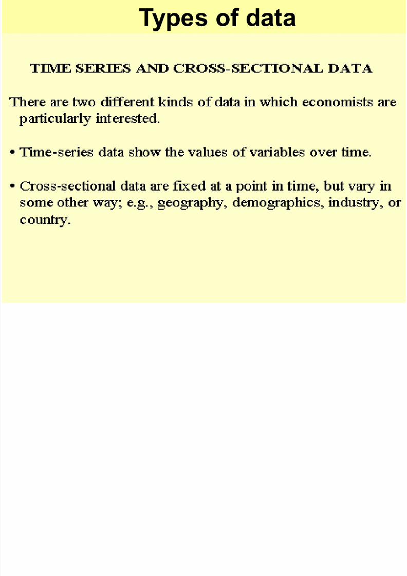
Types of data
8/11/2019 Demand Forecasting Information
http://slidepdf.com/reader/full/demand-forecasting-information 3/66
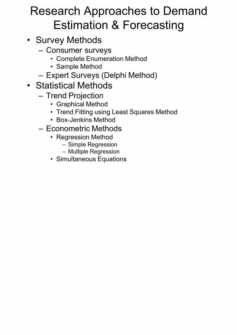
Research Approaches to Demand
Estimation & Forecasting
• Survey Methods – Consumer surveys
• Complete Enumeration Method
• Sample Method
– Expert Surveys (Delphi Method)
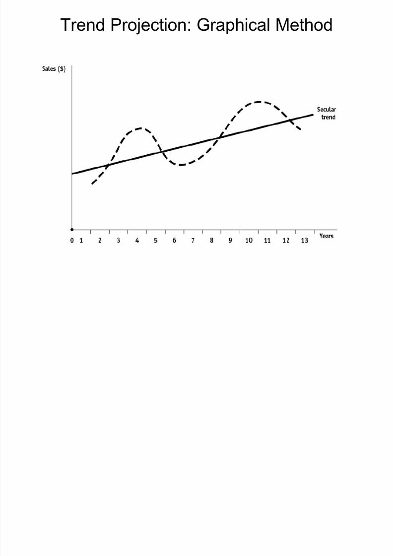
• Statistical Methods – Trend Projection
• Graphical Method
• Trend Fitting using Least Squares Method
• Box-Jenkins Method
– Econometric Methods• Regression Method
– Simple Regression
– Multiple Regression
• Simultaneous Equations

8/11/2019 Demand Forecasting Information
http://slidepdf.com/reader/full/demand-forecasting-information 4/66
Complete Enumeration Method
• Potential users are contacted and asked about their
future plan of purchasing the product.
If n out f m households in a city report the quantity
(d) they are willing to purchase of a commodity,
then total probable demand (Dp) will be
Dp = d1+d2+d3+….+dn
8/11/2019 Demand Forecasting Information
http://slidepdf.com/reader/full/demand-forecasting-information 5/66
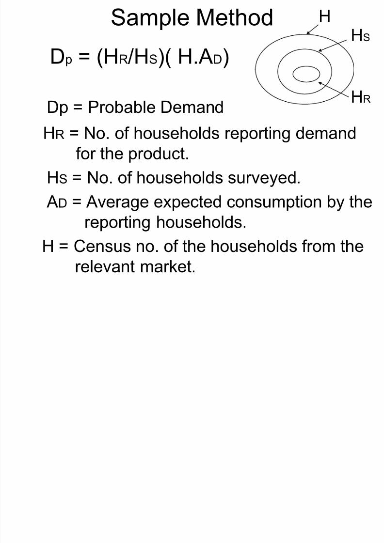
Sample Method
Dp
= (HR
/HS
)( H.AD
)
Dp = Probable Demand
HR = No. of households reporting demandfor the product.
HS = No. of households surveyed.
AD = Average expected consumption by thereporting households.
H = Census no. of the households from the
relevant market.
HHS
HR
8/11/2019 Demand Forecasting Information
http://slidepdf.com/reader/full/demand-forecasting-information 6/66
Delphi Method
Delphi method uses expert opinion about futuredevelopments. It was developed for long-range economicalpredictions by scientists of the Rand Corporation (1950s). It isan iterative process to collect and refine the anonymous
judgments of experts using a series of data collection andanalysis techniques interspersed with feedback.
The Delphi method is well suited as a research instrumentwhen there is incomplete knowledge about a problem orphenomenon. Feedback of results follows each step of
questioning. The process continues until no furtherconvergence of the experts' opinion is to be expected.
8/11/2019 Demand Forecasting Information
http://slidepdf.com/reader/full/demand-forecasting-information 7/66
Trend Projection: Graphical Method
8/11/2019 Demand Forecasting Information
http://slidepdf.com/reader/full/demand-forecasting-information 8/66
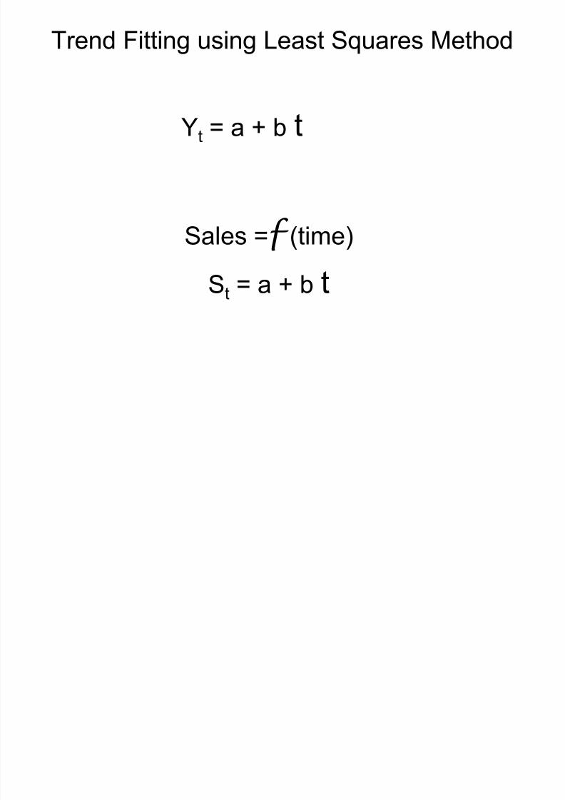
Trend Fitting using Least Squares Method
Yt = a + b t
Sales =f (time)
St = a + b t
8/11/2019 Demand Forecasting Information
http://slidepdf.com/reader/full/demand-forecasting-information 9/66
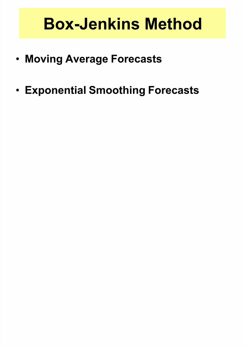
Box-Jenkins Method
• Moving Average Forecasts
• Exponential Smoothing Forecasts

8/11/2019 Demand Forecasting Information
http://slidepdf.com/reader/full/demand-forecasting-information 10/66
Moving Average Forecasts
Forecast is the average of data from w
periods prior to the forecast data point.
1
w
t i
t
i
A F
w

8/11/2019 Demand Forecasting Information
http://slidepdf.com/reader/full/demand-forecasting-information 11/66
Accuracy of a Forecasting Method
2( )t t A F
RMSE n
Root Mean Square Error (RMSE):
(Measures the accuracy of a forecasting Method)

8/11/2019 Demand Forecasting Information
http://slidepdf.com/reader/full/demand-forecasting-information 12/66
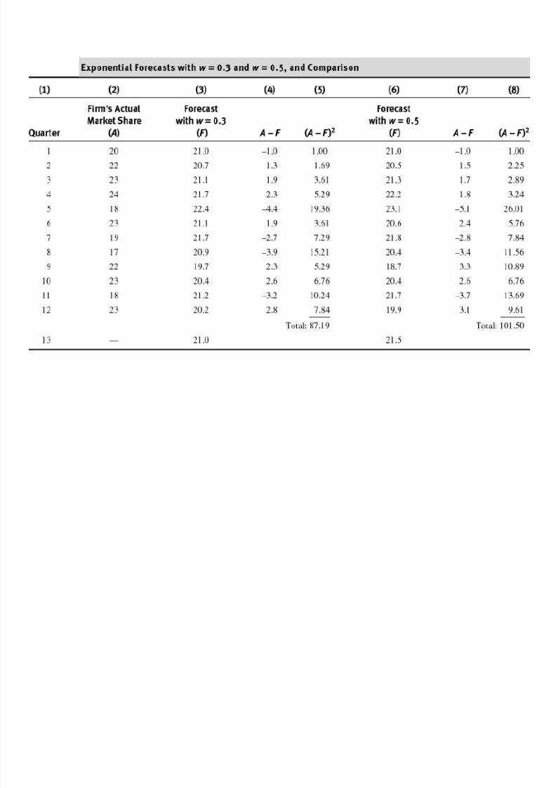
Three-quarter and Five-quarter Moving Average Forecast
?

8/11/2019 Demand Forecasting Information
http://slidepdf.com/reader/full/demand-forecasting-information 13/66
8/11/2019 Demand Forecasting Information
http://slidepdf.com/reader/full/demand-forecasting-information 14/66
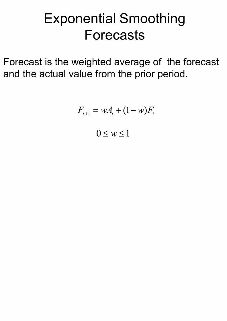
Exponential Smoothing
Forecasts
1 (1 )t t t F wA w F
Forecast is the weighted average of the forecast
and the actual value from the prior period.
0 1w

8/11/2019 Demand Forecasting Information
http://slidepdf.com/reader/full/demand-forecasting-information 15/66
Root Mean Square Error
2( )t t A F RMSE
n
To measure the accuracy of the forecast
8/11/2019 Demand Forecasting Information
http://slidepdf.com/reader/full/demand-forecasting-information 16/66

8/11/2019 Demand Forecasting Information
http://slidepdf.com/reader/full/demand-forecasting-information 17/66
Regression Analysis
8/11/2019 Demand Forecasting Information
http://slidepdf.com/reader/full/demand-forecasting-information 18/66
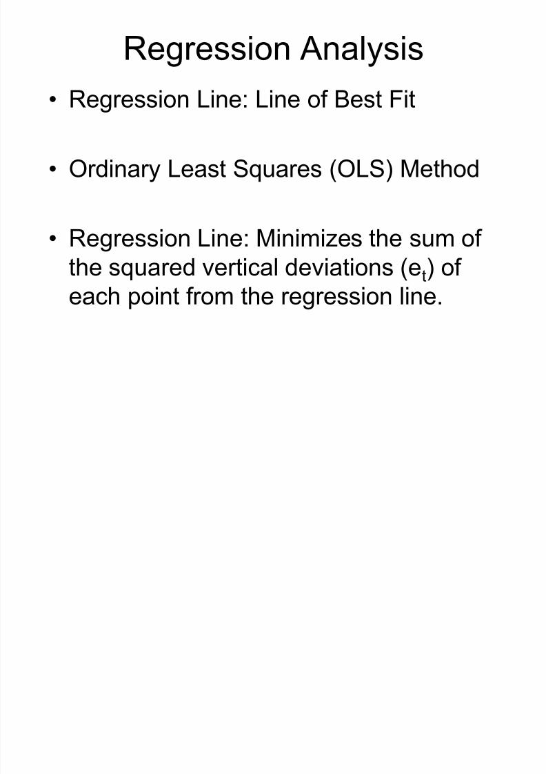
Regression Analysis
• Regression Line: Line of Best Fit
• Ordinary Least Squares (OLS) Method
• Regression Line: Minimizes the sum of
the squared vertical deviations (et) of
each point from the regression line.

8/11/2019 Demand Forecasting Information
http://slidepdf.com/reader/full/demand-forecasting-information 19/66
8/11/2019 Demand Forecasting Information
http://slidepdf.com/reader/full/demand-forecasting-information 20/66
8/11/2019 Demand Forecasting Information
http://slidepdf.com/reader/full/demand-forecasting-information 21/66
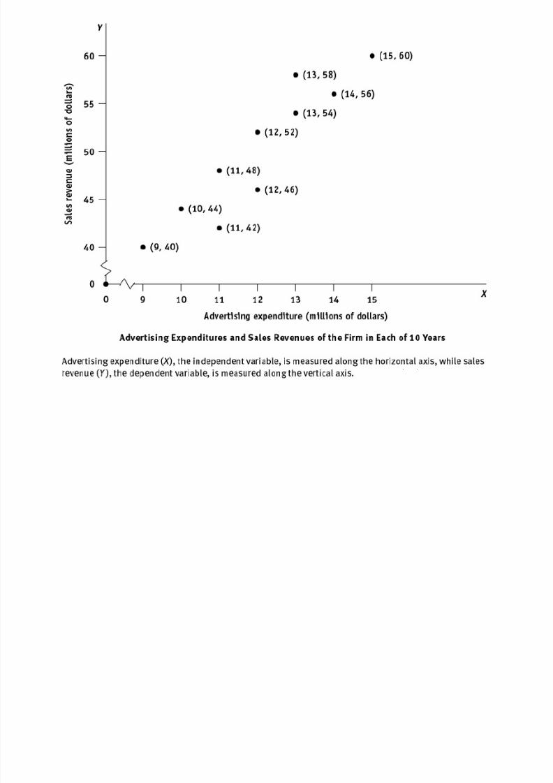
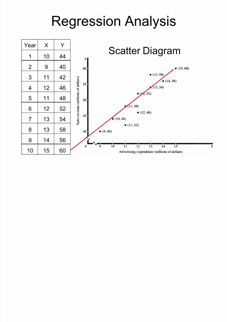
Scatter Diagram
Regression Analysis
Year X Y
1 10 44
2 9 40
3 11 42
4 12 46
5 11 48
6 12 52
7 13 54
8 13 58
9 14 56
10 15 60

8/11/2019 Demand Forecasting Information
http://slidepdf.com/reader/full/demand-forecasting-information 22/66

8/11/2019 Demand Forecasting Information
http://slidepdf.com/reader/full/demand-forecasting-information 23/66
Ordinary Least Squares (OLS)
Model: t t t Y a bX e
ˆˆ ˆt t Y a bX
ˆ
t t t
e Y Y
Properties:
(i) = 0
(ii) is minimum.

8/11/2019 Demand Forecasting Information
http://slidepdf.com/reader/full/demand-forecasting-information 24/66
Ordinary Least Squares (OLS)
Objective: Determine the slope and intercept
that minimize the sum of the squared errors.
2 2 2
1 1 1
ˆˆ ˆ( ) ( )n n n
t t t t t
t t t
e Y Y Y a bX
Method used for this: Maxima Minima
8/11/2019 Demand Forecasting Information
http://slidepdf.com/reader/full/demand-forecasting-information 25/66
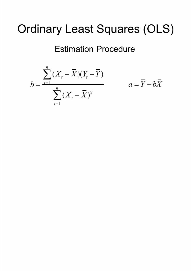
Ordinary Least Squares (OLS)Estimation Procedure
1
2
1
( )( )ˆ
( )
n
t t
t
n
t
t
X X Y Y
b
X X
ˆa Y bX
f

8/11/2019 Demand Forecasting Information
http://slidepdf.com/reader/full/demand-forecasting-information 26/66
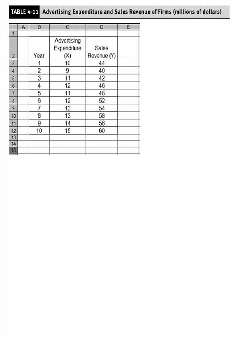
Data on sales and Advertising expenditure for 10
years for a firm.
Year Ad. Expenses Sales 1 10 44
2 9 40
3 11 42
4 12 46 5 11 48
6 12 52
7 13 54
8 13 58 9 14 56
10 15 60
8/11/2019 Demand Forecasting Information
http://slidepdf.com/reader/full/demand-forecasting-information 27/66
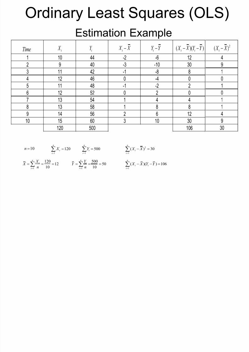
Ordinary Least Squares (OLS)
Estimation Example
1 10 44 -2 -6 12
2 9 40 -3 -10 30
3 11 42 -1 -8 8
4 12 46 0 -4 0
5 11 48 -1 -2 2
6 12 52 0 2 0
7 13 54 1 4 4
8 13 58 1 8 8
9 14 56 2 6 12
10 15 60 3 10 30
120 500 106
4
9
1
0
1
0
1
1
4
9
30
Time t X
t Y
t X X
t Y Y ( )( )
t t X X Y Y
2( )
t X X
10n
1
12012
10
nt
t
X X
n
1
50050
10
nt
t
Y Y
n
1
120n
t
t
X
1
500n
t
t
Y
2
1
( ) 30n
t
t
X X
1
( )( ) 106n
t t
t
X X Y Y
8/11/2019 Demand Forecasting Information
http://slidepdf.com/reader/full/demand-forecasting-information 28/66
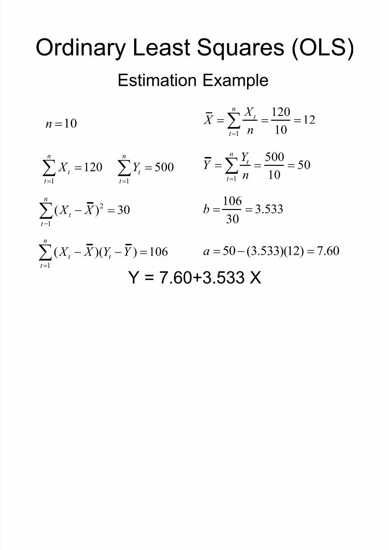
Ordinary Least Squares (OLS)
Estimation Example
10n 1
12012
10
nt
t
X X
n
1
50050
10
nt
t
Y Y
n
1
120n
t
t
X
1
500n
t
t
Y
2
1
( ) 30n
t
t
X X
1
( )( ) 106n
t t
t
X X Y Y
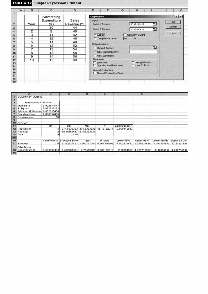
106ˆ 3.53330
b
ˆ 50 (3.533)(12) 7.60a
Y = 7.60+3.533 X

8/11/2019 Demand Forecasting Information
http://slidepdf.com/reader/full/demand-forecasting-information 29/66
Y = 7.60+3.533 X
Tests of significance?
8/11/2019 Demand Forecasting Information
http://slidepdf.com/reader/full/demand-forecasting-information 30/66

8/11/2019 Demand Forecasting Information
http://slidepdf.com/reader/full/demand-forecasting-information 31/66
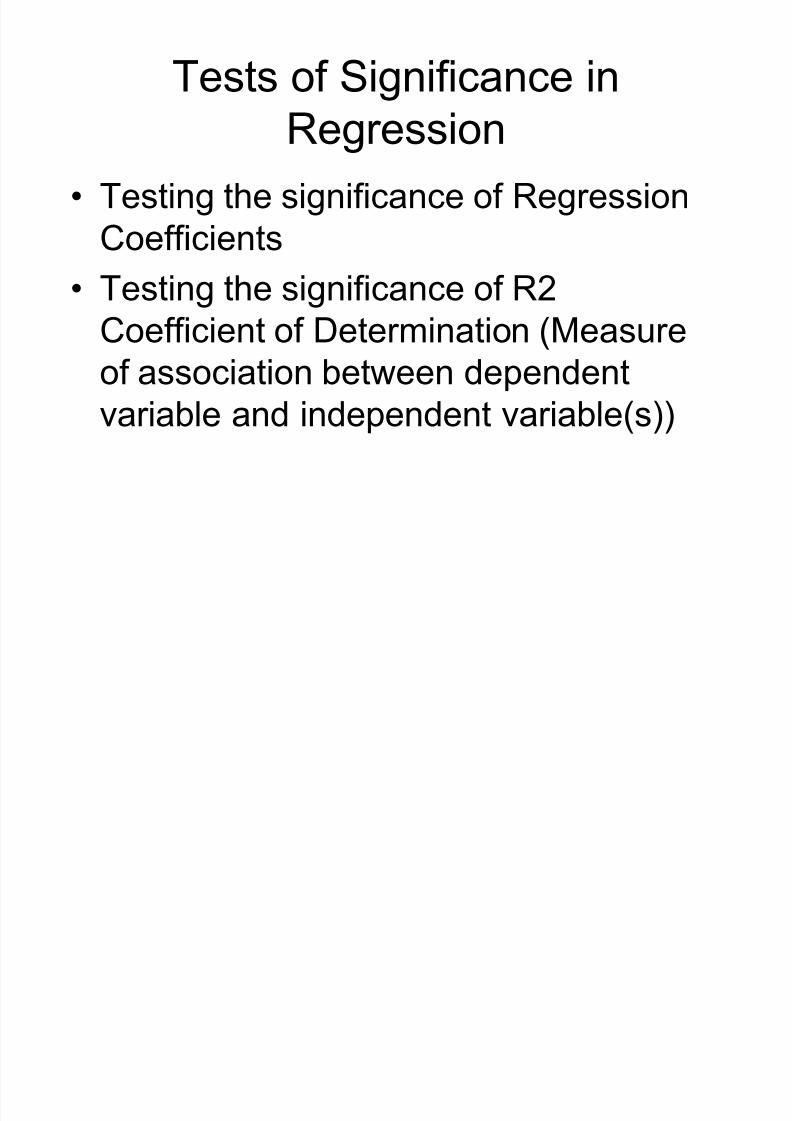
Test for Significance
Under the validity of H 0 , t statistic will be used,
where
SE b denotes the standard deviation of b and
is called the standard error .
H0: 1 = 0H1: 1 0
t = b
SE b
α = 0.05
With d.f. = n-2

8/11/2019 Demand Forecasting Information
http://slidepdf.com/reader/full/demand-forecasting-information 32/66
Standard Error of the Slope Estimate (b)
2 2
ˆ 2 2
ˆ
( )( ) ( ) ( ) ( )
t t
b
t t
Y Y e s
n k X X n k X X
(k -1) (k -1)

8/11/2019 Demand Forecasting Information
http://slidepdf.com/reader/full/demand-forecasting-information 33/66
Tests of Significance
2 2
1 1
ˆ( ) 65.4830n n
t t t
t t
e Y Y
2
1
( ) 30n
t
t
X X
2
ˆ 2
ˆ( ) 65.48300.52
( ) ( ) (10 2)(30)
t
bt
Y Y s
n k X X
1 10 44 42.90
2 9 40 39.37
3 11 42 46.43
4 12 46 49.96
5 11 48 46.43
6 12 52 49.96
7 13 54 53.49
8 13 58 53.49
9 14 56 57.02
10 15 60 60.55
1.10 1.2100 4
0.63 0.3969 9
-4.43 19.6249 1
-3.96 15.6816 0
1.57 2.4649 1
2.04 4.1616 0
0.51 0.2601 1
4.51 20.3401 1
-1.02 1.0404 4
-0.55 0.3025 9
65.4830 30
Time t
X t
Y ˆt
Y ˆt t t
e Y Y 2 2ˆ
( )t t t e Y Y
2
( )t X X
8/11/2019 Demand Forecasting Information
http://slidepdf.com/reader/full/demand-forecasting-information 34/66
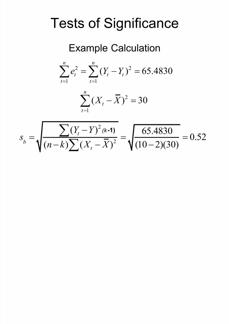
Tests of Significance
Example Calculation
2
ˆ 2
ˆ( ) 65.48300.52
( ) ( ) (10 2)(30)
t
bt
Y Y s
n k X X
2
1
( ) 30n
t
t
X X
2 2
1 1
ˆ( ) 65.4830n n
t t t
t t
e Y Y
(k -1)
T t f Si ifi
8/11/2019 Demand Forecasting Information
http://slidepdf.com/reader/full/demand-forecasting-information 35/66
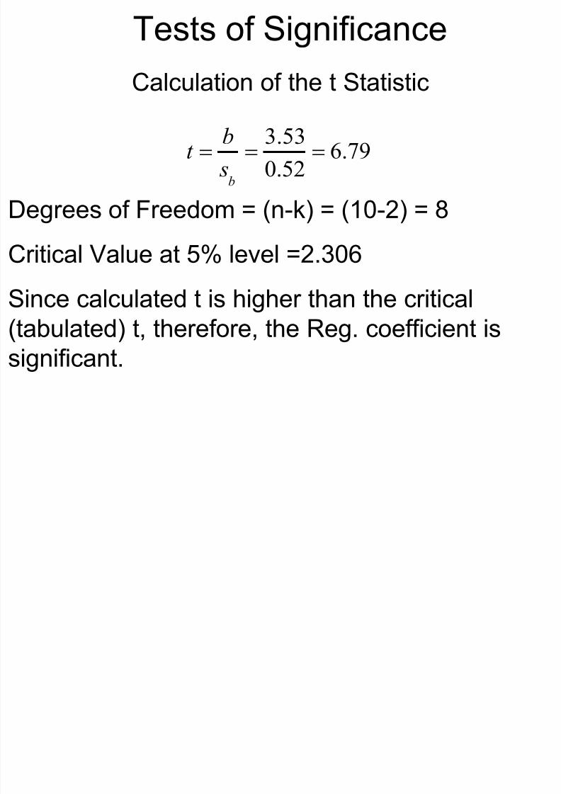
Tests of Significance
Calculation of the t Statistic
ˆ
ˆ 3.536.79
0.52b
bt
s
Degrees of Freedom = (n-k) = (10-2) = 8
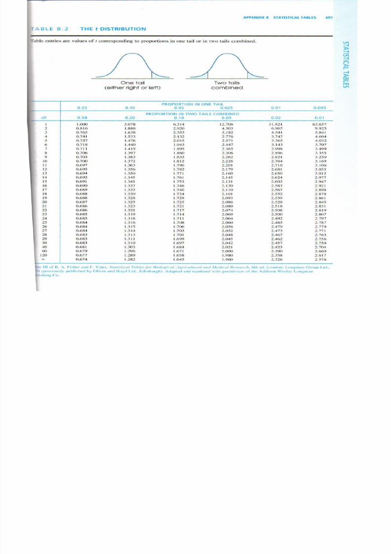
Critical Value at 5% level =2.306
Since calculated t is higher than the critical(tabulated) t, therefore, the Reg. coefficient is
significant.

8/11/2019 Demand Forecasting Information
http://slidepdf.com/reader/full/demand-forecasting-information 36/66
Y = 7.60+3.533 X
Hence we can say that b is a significant
regression coefficient which infers thatX is a significant explanatory variable
for Y.
8/11/2019 Demand Forecasting Information
http://slidepdf.com/reader/full/demand-forecasting-information 37/66
8/11/2019 Demand Forecasting Information
http://slidepdf.com/reader/full/demand-forecasting-information 38/66
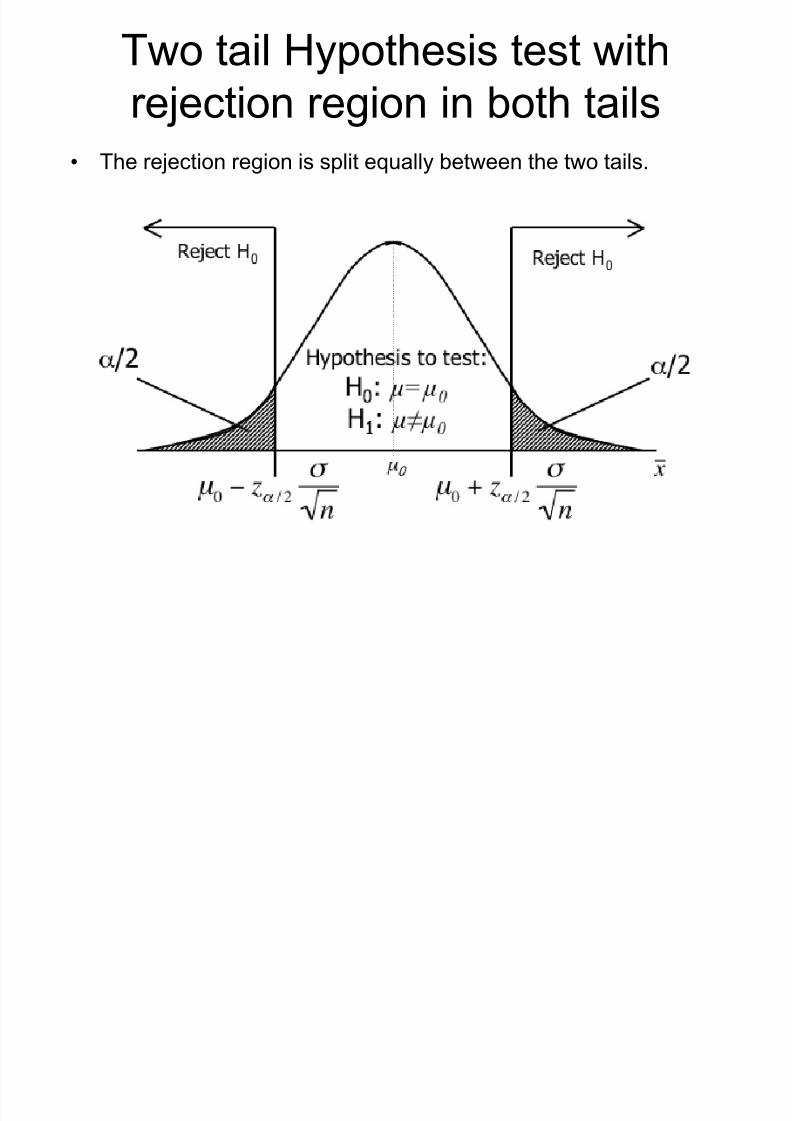
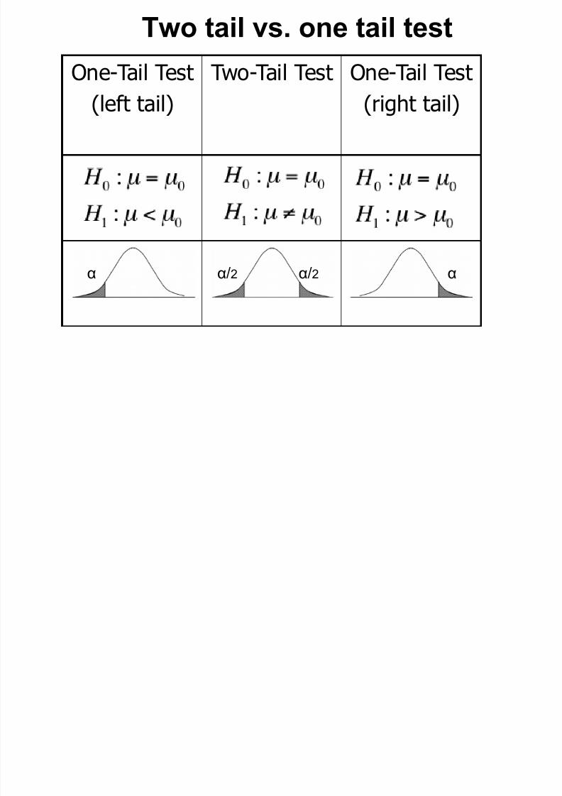
Two tail Hypothesis test with
rejection region in both tails
• The rejection region is split equally between the two tails.
T t il t il t t
8/11/2019 Demand Forecasting Information
http://slidepdf.com/reader/full/demand-forecasting-information 39/66
One-Tail Test
(left tail)
Two-Tail Test One-Tail Test
(right tail)
Two tail vs. one tail test
α α α/2 α/2

8/11/2019 Demand Forecasting Information
http://slidepdf.com/reader/full/demand-forecasting-information 40/66
Test of Significance of R2

8/11/2019 Demand Forecasting Information
http://slidepdf.com/reader/full/demand-forecasting-information 41/66
Decomposition of Variation in Dependent
Variable
2 2 2ˆ ˆ( ) ( ) ( )t t t Y Y Y Y Y Y
Total Variation = Explained Variation + Unexplained
Variation
n-1 = k-1 + n-k

8/11/2019 Demand Forecasting Information
http://slidepdf.com/reader/full/demand-forecasting-information 42/66

8/11/2019 Demand Forecasting Information
http://slidepdf.com/reader/full/demand-forecasting-information 43/66
Test of Significance
Coefficient of Determination
2
22
ˆ( )
( )t
Y Y Explained Variation R Total Variation Y Y
2 373.84
0.85440.00 R

8/11/2019 Demand Forecasting Information
http://slidepdf.com/reader/full/demand-forecasting-information 44/66
Significance of Coefficient of Determination

8/11/2019 Demand Forecasting Information
http://slidepdf.com/reader/full/demand-forecasting-information 45/66
Significance of Coefficient of Determination
H0: R 2 = 0
H1: R 2 > 0
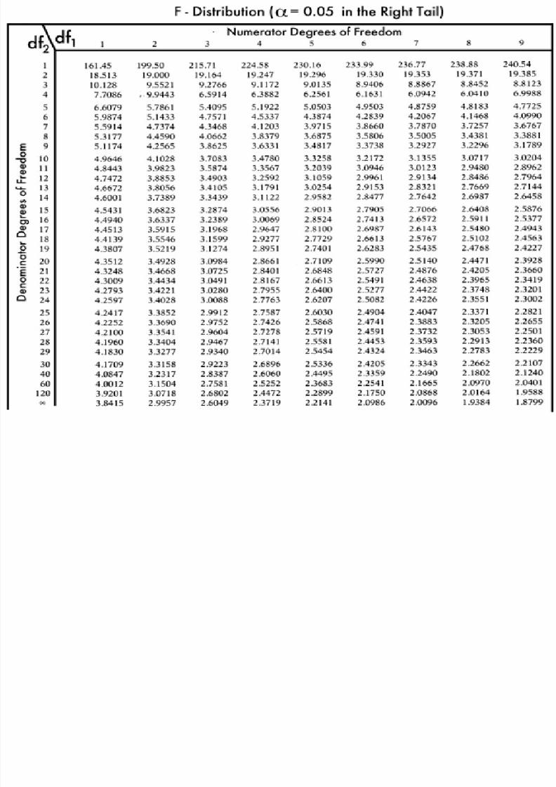
Under the validity of H0, the appropriate test statistic is the F statistic:
which has an F distribution with 1 and n - 2 degrees of freedom.
F = S SR /(k-1)
S SE / ( n -k )
05.0

8/11/2019 Demand Forecasting Information
http://slidepdf.com/reader/full/demand-forecasting-information 46/66
Source Sum of Squares D.F. Mean Square F
Regression SSR k-1
Error SSE n-k
Total SST n-1
If is accepted,
otherwise significant regression.
1
k
SSR MSR
k n
SSE MSE
MSE
MSR F
k nk
F F
,1
ANOVA Table

8/11/2019 Demand Forecasting Information
http://slidepdf.com/reader/full/demand-forecasting-information 47/66
8/11/2019 Demand Forecasting Information
http://slidepdf.com/reader/full/demand-forecasting-information 48/66
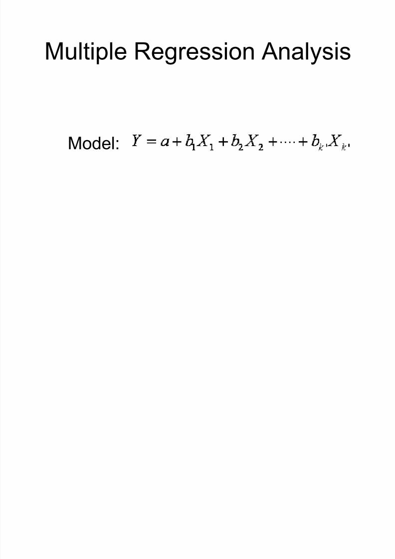
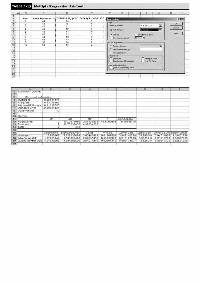
Multiple Regression Analysis
Model:

8/11/2019 Demand Forecasting Information
http://slidepdf.com/reader/full/demand-forecasting-information 49/66

8/11/2019 Demand Forecasting Information
http://slidepdf.com/reader/full/demand-forecasting-information 50/66
Multiple Regression Analysis
Analysis of Variance and F Statistic
/( 1)
/( )
Explained Variation k F
Unexplained Variation n k
2
2
/( 1)
(1 ) /( )
R k F
R n k
Significance Testing of Overall

8/11/2019 Demand Forecasting Information
http://slidepdf.com/reader/full/demand-forecasting-information 51/66
Significance Testing of Overall
Regression
H0 : R 2 = 0
This is equivalent to the following null hypothesis:
H0: 1 = 2 = 3 = . . . = k = 0
The overall test can be conducted by using an F statistic:
R 2 / K-1 ( 1 - R 2 ) / ( n - k)
which has an F distribution with k-1 and (n - k ) degrees of freedom.
F =
8/11/2019 Demand Forecasting Information
http://slidepdf.com/reader/full/demand-forecasting-information 52/66

8/11/2019 Demand Forecasting Information
http://slidepdf.com/reader/full/demand-forecasting-information 53/66
Problems in Regression Analysis
• Multicollinearity: Two or more
explanatory variables are highly
correlated.• Heteroscedasticity: Variance of error
term is not independent of the Y
variable.• Autocorrelation: Consecutive error
terms are correlated.

8/11/2019 Demand Forecasting Information
http://slidepdf.com/reader/full/demand-forecasting-information 54/66
Multicollinearity (MC)
8/11/2019 Demand Forecasting Information
http://slidepdf.com/reader/full/demand-forecasting-information 55/66
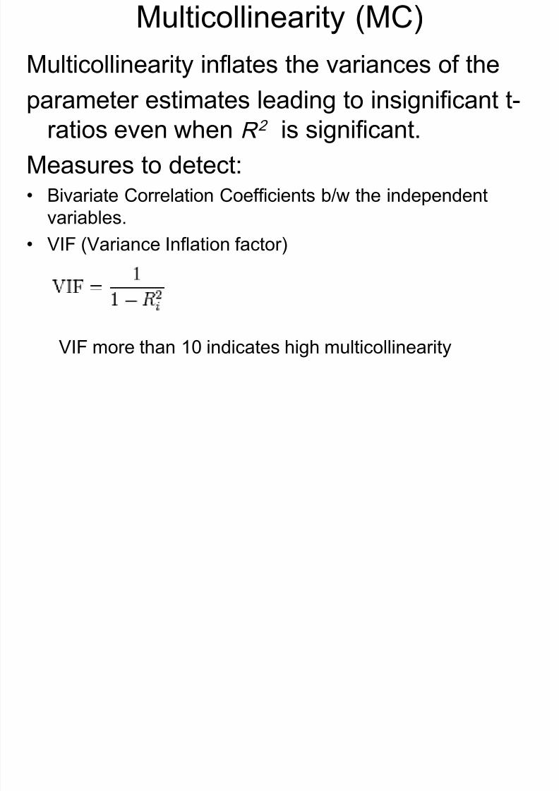
Multicollinearity (MC)
Multicollinearity inflates the variances of the
parameter estimates leading to insignificant t-ratios even when R 2 is significant.
Measures to detect:
• Bivariate Correlation Coefficients b/w the independentvariables.
• VIF (Variance Inflation factor)
VIF more than 10 indicates high multicollinearity
Remedial Measures for MC
8/11/2019 Demand Forecasting Information
http://slidepdf.com/reader/full/demand-forecasting-information 56/66
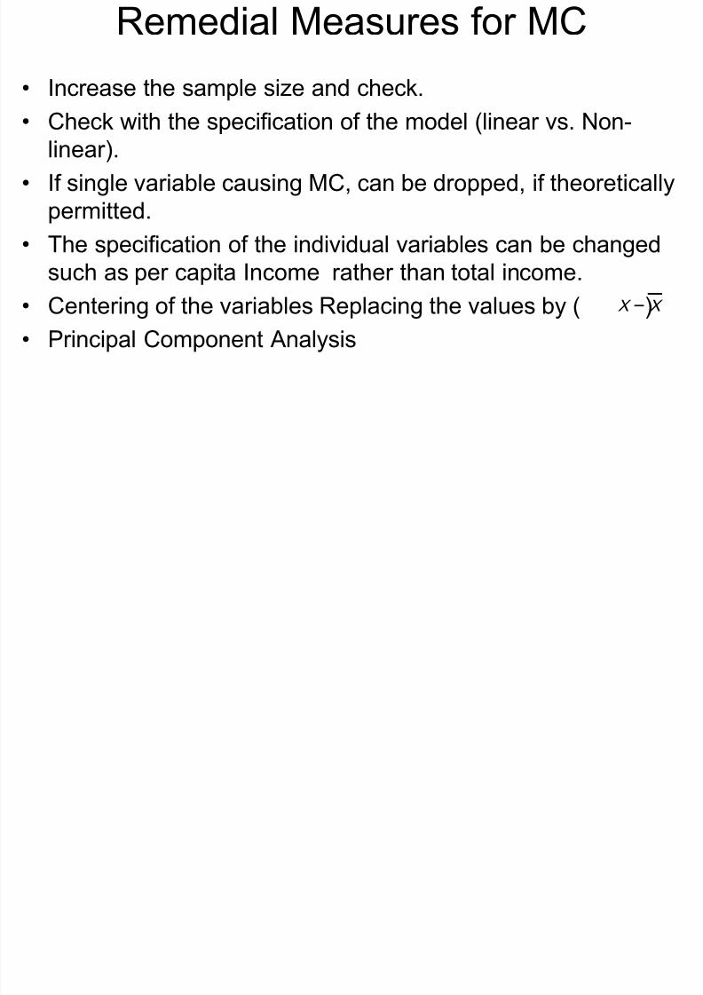
Remedial Measures for MC
• Increase the sample size and check.
• Check with the specification of the model (linear vs. Non-linear).
• If single variable causing MC, can be dropped, if theoretically
permitted.
• The specification of the individual variables can be changedsuch as per capita Income rather than total income.
• Centering of the variables Replacing the values by ( )
• Principal Component Analysis
X X
Durbin Watson Statistic
8/11/2019 Demand Forecasting Information
http://slidepdf.com/reader/full/demand-forecasting-information 57/66
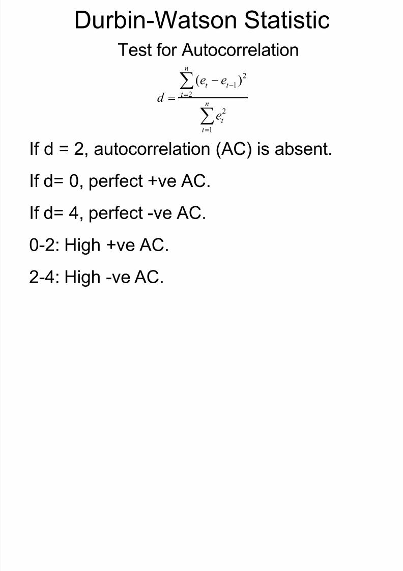
Durbin-Watson StatisticTest for Autocorrelation
21
2
2
1
( )n
t t
t
n
t
t
e e
d
e
If d = 2, autocorrelation (AC) is absent.
If d= 0, perfect +ve AC.
If d= 4, perfect -ve AC.
0-2: High +ve AC.
2-4: High -ve AC.

8/11/2019 Demand Forecasting Information
http://slidepdf.com/reader/full/demand-forecasting-information 58/66
H0: R= 0
8/11/2019 Demand Forecasting Information
http://slidepdf.com/reader/full/demand-forecasting-information 59/66
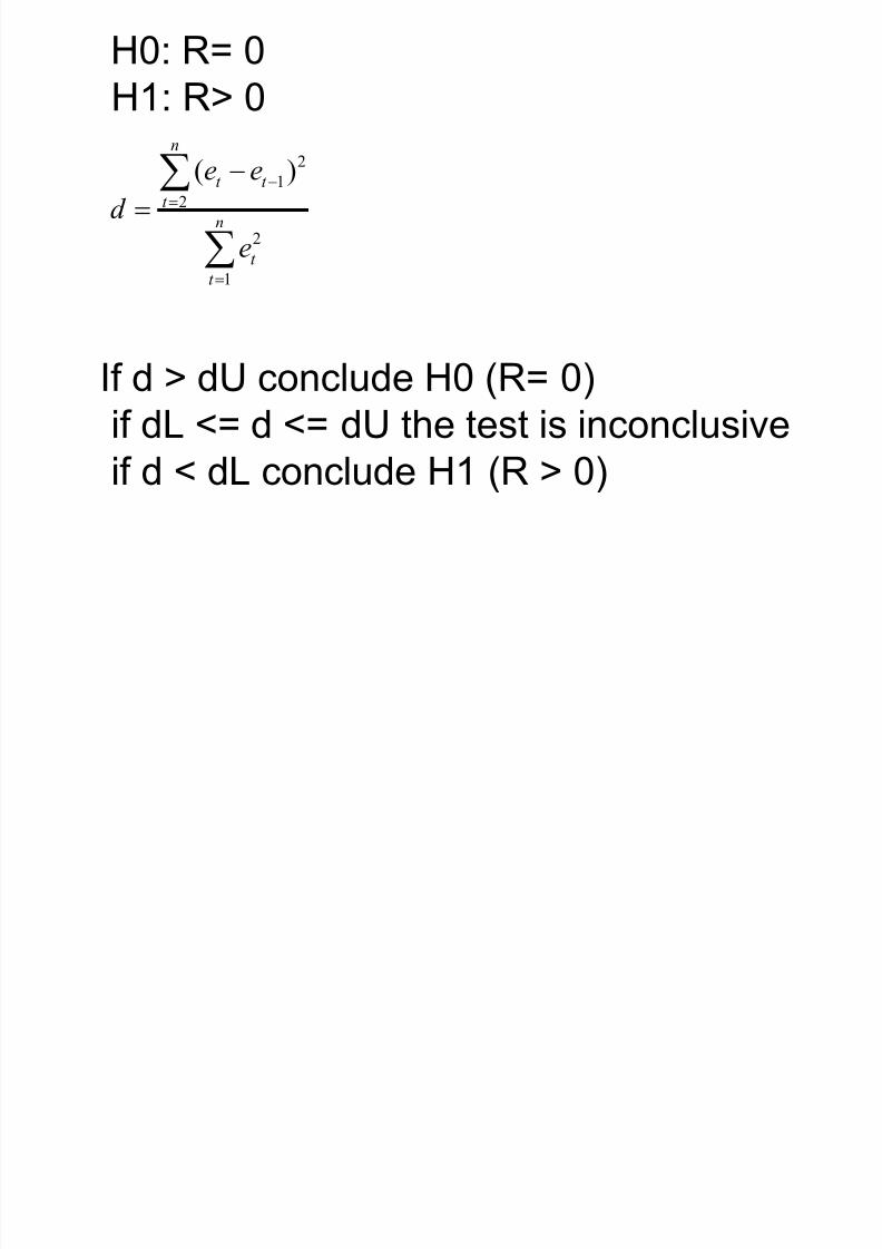
H0: R= 0
H1: R> 0
If d > dU conclude H0 (R= 0)
if dL <= d <= dU the test is inconclusive
if d < dL conclude H1 (R > 0)
21
2
2
1
( )
n
t t
t
n
t
t
e e
d
e
8/11/2019 Demand Forecasting Information
http://slidepdf.com/reader/full/demand-forecasting-information 60/66
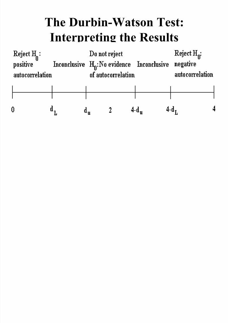
The Durbin-Watson Test:
Interpreting the Results
D-W Statistic Table

8/11/2019 Demand Forecasting Information
http://slidepdf.com/reader/full/demand-forecasting-information 61/66
No. of independent variables

8/11/2019 Demand Forecasting Information
http://slidepdf.com/reader/full/demand-forecasting-information 62/66
Steps in Demand Estimation
• Model Specification: Identify Variables
• Collect Data
• Specify Functional Form
• Estimate Function
• Test the Results
F ti l F S ifi ti
8/11/2019 Demand Forecasting Information
http://slidepdf.com/reader/full/demand-forecasting-information 63/66
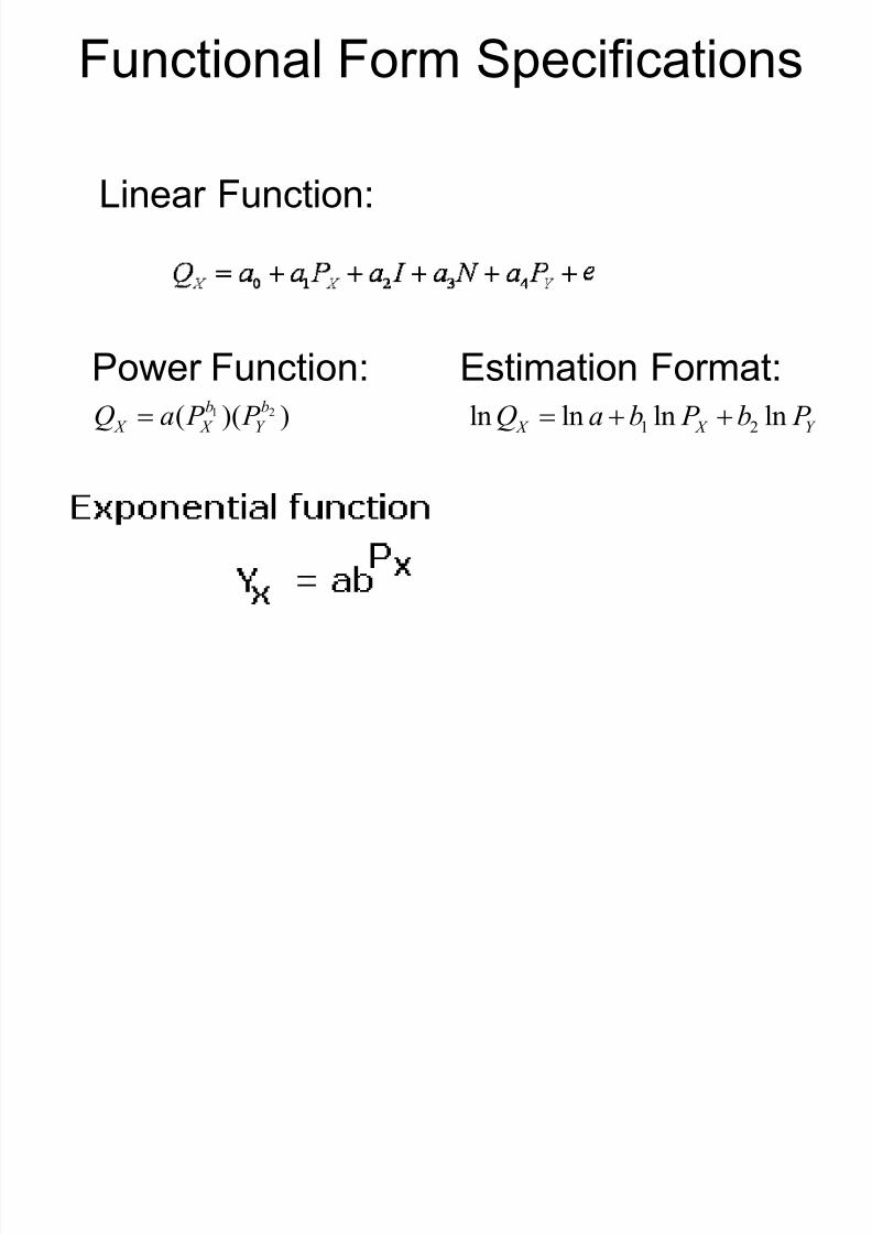
Functional Form Specifications
Linear Function:
Power Function:1 2( )( )b b
X X Y Q a P P
Estimation Format:
1 2ln ln ln ln X X Y Q a b P b P
8/11/2019 Demand Forecasting Information
http://slidepdf.com/reader/full/demand-forecasting-information 64/66
8/11/2019 Demand Forecasting Information
http://slidepdf.com/reader/full/demand-forecasting-information 65/66
8/11/2019 Demand Forecasting Information
http://slidepdf.com/reader/full/demand-forecasting-information 66/66