DEMAND RESPONSE FOR RESIDENTIALUSES: A DATA ANALYTICS APPROACH*

Abdelkareem Jaradat, Hanan Lutfiyya, Anwar HaqueDepartment of Computer ScienceThe University of Western Ontario

London, Canada{ajarada3, hlutfiyy, ahaque32}@uwo.ca

Abstract—In the Smart Grid environment, the advent ofintelligent measuring devices facilitates monitoring applianceelectricity consumption. This data can be used in applying De-mand Response (DR) in residential houses through data analytics,and developing data mining techniques. In this research, weintroduce a smart system foundation that is applied to user’sdisaggregated power consumption data. This system encouragesthe users to apply DR by changing their behaviour of usingheavier operation modes to lighter modes, and by encouragingusers to shift their usages to off-peak hours. First, we applyCross Correlation (XCORR) to detect times of the occurrenceswhen an appliance is being used. We then use The Dynamic TimeWarping (DTW) [13] algorithm to recognize the operation modeused.

Index Terms—Dynamic Time Warping (DTW), Smart Systems,Time-Series Analysis, Smart Grid, Disaggregated Power Con-sumption, Demand Response, IoT

I. INTRODUCTION

Demand Response (DR) is used to lower the demand onpower systems by having consumers reduce or shift theirpower usage [17]. Demand response may be used to increasedemand during periods of high supply and low demand. DRis considered a more cost-effective option than building morepower stations [3]. Demand response is not a new concept,but in most countries it still plays a limited role [16]. Onechallenge is that although power consumption for residentialpurposes accounts for 40% or more of overall power consump-tion, DR techniques have been ineffective [11]. One reason isthat most of the programs for residential demand responsefocus on a single value of power consumption representingthe total power consumption [6]. However, overall residentialpower consumption is generated by a diverse set of powerconsuming devices that includes cooling and heating units,washing machines, dryers, refrigerators, lighting, etc. Theusage of many of the individual appliances can be adjusted.The diverse nature of devices that consume power suggeststhat a single value of power consumption representing theaggregation of the values of different devices that consumepower is unsuitable. There has been relatively little work thatconsiders disaggregated demand.

* We would like to thank the Natural Sciences and Engineering ResearchCouncil of Canada (NSERC) for their support through the Strategic GrantsProgram.

With smart meters and sensors that can measure powerconsumption per appliance it has become much easier tomonitor power consumption per device. In the work presentedin this paper, we are particularly interested in being able todetect the start and end time of an appliance usage as wellas the operation mode being used. Each operation mode ischaracterized by its running time and different cycles thatthe appliance can run in. Activating an appliance in a certainoperation mode consumes energy differently than other modes.Therefore, DR could be applied based on the outcomes of thisanalysis by first, finding the activation times of appliances.The power consumption data is processed in order to find theturn on times for the appliance. We obtain the time when thehigh load starts. Consequently, a recommendation could besent to the consumer if the detected time falls within the on-peak time advising the consumer to shift the load either beforeor after the current time to avoid higher energy prices. Second,recognizing the operation mode of each appliance activation.Most of modern appliances have the option to run in differentoperation modes. For example, a washing machine could beprogrammed with three or four different operation modes.Each of these modes runs the inner components of the washingmachine differently. Also, every mode has its own timing andcycles activated in different power levels during the runningtime. By determining these cycles, a model could be formedfor each operation mode. This has the potential to serve as thefoundation for a smart recommendation system that appliesDR to provide consumers with recommendations about theirconsumption for different appliances. These recommendationscome into place after applying the detection of appliance acti-vation and the recognition of operation modes in such way toencourage the residents to shift their usages to off-peak periodsof the day, when power is cheaper. Also the recommendationscould advise consumers to change their behaviour of usinglighter operation modes with less consumption.

The rest of the paper is organized as the following: Insection II we discuss previous work that addresses eventdetection and classification. Section III discusses the dataanalysis of the power consumption. In section IV we presenta detection algorithm. Section V discusses the algorithm toclassify appliances operation modes. Section VI discussesthe process of simulating power consumption. Section VIIdiscusses the results and section VIII concludes the paper.

arX

iv:2

008.

0290

8v1

[ee

ss.S

P] 7

Aug

202

0

II. RELATED WORK

The literature describes many techniques used to analyzethe electricity consumption data so that end user applicationscould be built on top of these approaches. These techniquesprimarily concerned with event detection and event classifica-tion in time series data. Typically the event is the activationand deactivation of appliances during its operation with thepower distribution over time. This serves in defining attributesto target customers for appliance specific application with DR.

A. Event Detection

Event detection algorithms are used to detect load profiles.A load profile is the power distribution in a form of cycles overa single run for an appliance. Event detection is concerned withfinding transition states for loads/appliances from aggregatedpower consumption data. Each transition state is characterizedby a sudden change in the power value, which indicatesactivating an appliance or a change in the running cycle.Based on the determined timing for the transitions, load profileare extracted separately. This is what is referred to as Non-Intrusive Load Monitoring (NILM) [19].

Matched Filters methods involve a known signal (templatesignal) to be correlated with an unknown signal to detect theoccurrence of the template in the unknown signal. Rueda et.al.[14] proposed a matched filter detection approach by convolv-ing the appliance consumption signal with a conjugated time-reversed version of a manually extracted template. Baets et.al.[2] presented an event detection method that uses CepstrumAnalysis in the frequency domain. Alcala et.al. [1] proposedan approach using Hilbert Transform to extract the envelope ofthe current signal. Then, by using Average Filters, DerivationFilters, and thresholding to cut off the signal, transition eventsare detected.

B. Event Classification

Different approaches are concerned with classifying loadsignature extracted from aggregated power consumption datainto the individual appliance/load. Liao et.al. [4] proposed anapproach for appliance load classification using Dynamic TimeWarping (DTW). Tang et.al. [15] designed the Sparse HumanAction Recovery with Knowledge of appliances (SHARK)framework. It is an occupancy detection framework that is non-intrusive and requires no training process. Liu et.al. [5] used aNearest Neighbor Transient Identification method to identifythe appliance creating the Transient Power Waveform (TPW)sample time-series, then the DTW-based integrated distanceis utilized to calculate the similarity of TPW signatures anda template time series for an appliance. Wang et.al. [18]describes an approach which uses Iterative Disaggregationbased on Appliance Consumption Pattern (ILDACP). Thisapproach combines Fuzzy C-means clustering algorithm todetect appliance operating status, and DTW search that identi-fies single energy consumption based on the appliance typicalpower consumption pattern (a template pattern).

Sep 14 Sep 19 Sep 24 Sep 29 Oct 4 Oct 9 Oct 14 Oct 19 Oct 24 Oct 29 Nov 3 Nov 8 Nov 13 Time [2017]

0

100

200

300

400

500

Pow

er (W

)

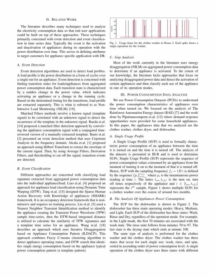
Fig. 1. Usage times for the clothes washer in House 2. Each spike shows asingle operation for the washer.

C. Gap Analysis

Most of the work currently in the literature uses energydisaggregation (NILM) on aggregated power consumption datato determine if an appliance is activated. To the extent ofour knowledge, the literature lacks approaches that focus onanalyzing disaggregated power data and detect the activation ofcertain appliances and then classify each use of the appliancein one of its operation modes.

III. POWER CONSUMPTION DATA ANALYSIS

We use Power Consumption Datasets (PCDs) to understandthe power consumption characteristics of appliances overtime when turned on. We focused on the analysis of TheRainforest Automation Energy dataset (RAE) [7] and the workdone by Pipattanasomporn et.al. [12] where demand responseopportunities were provided for some household appliances.In this paper, the appliances data that we analyzed are theclothes washer, clothes dryer, and dishwasher.

A. Single Usage Profile

A Single Usage Profile (SUP) is used to formally charac-terize power consumption of an appliance between the timeit is turned on and the time it is turned off. The analysis ofthe datasets is presented in III-B and is used to determineSUPs. Single Usage Profile (SUP) represents the sequence ofpower consumption values consumed by an appliance from themoment of turning it on to the moment of that it is turned off.Hence, SUP with the sampling frequency fs = 1Hz is definedby the sequence {pi}

toff

i=tonwhere pi is the instantaneous power

reading at time i. The times ton, toff is the turn on, turnoff times respectively of the appliance and i ∈ [ton, toff ]represents the ith sample. Figure 1 shows multiple SUPs fora clothes washer over the course of around two months.

B. The Analysis Of Appliances Power Consumption

The SUP for the dishwasher is shown in Figure 2. Thedishwasher has three main operating modes: Heavy, Medium,and Light. Each SUP of the dishwasher has three states: Wash,Rinse and Dry, regardless of the operation mode. For example,in the Light mode, the first 70 minutes are associated with thewash state. The rinse state follows from minutes 70 to 97. Thelast state is the drying state which ends at minute 108.

The same type of analysis is performed for the clotheswasher and the clothes dryer. The clothes washer has threestates that occur for each single use: wash, rinse, and spin,sorted in ascending order of power consumption level. A singleoperation of the clothes dryer uses three states with different

Time

0

1000

0

1000

Pow

er (W

)

1000

(a) Heavy

(b) Medium

(c) LightDryRinseWash

12:00AM 12:20AM 12:40AM 1:00AM 1:20AM 1:40AM 2:00AM 2:20AM 2:40AM 3:00AM

Fig. 2. Single Usage Profile (SUP) for the dishwasher showing three operationmodes: (a) Heavy, (b) Medium, (c) Light.

temperatures: Maximum Heat, Medium Heat, No Heat. Duringthe Maximum Heat state the dryer drum is heated to themaximum temperature in the dryer setting, and so on for theother states.

By analyzing appliances data, we found similar patterns.Each activation with certain operation mode has a specificpattern of consumption based on the states of the appliance.These states are preconfigured by the manufacturer in termsof timing and power consumption levels.

IV. SINGLE USE PROFILE DETECTION

With Demand Response, consumers are encouraged to useappliances in off peak hours. This requires the need to detectwhen appliances are activated. Hence, we can advice the userto shift the load or not based on the detected time. Thisserves as a basis for further analysis in determining applianceoperation modes.

A. The Reference Pattern

We use a Reference Pattern (RP) which represents the startof a SUP. RP is a sequence of data points represented as S(t)which returns the data point that represents the power valueassociated with t. We focus on matching RP to a subsequenceof the daily time series which is represented by D(t). RPis derived from a generated SUP by taking a slice of thegenerated SUP corresponding to turning on the appliance.

B. Cross Correlation

In time series analysis, Cross Correlation (XCORR) [8] isa measure of similarity of two series as a function of thedisplacement of one series relative to the other series. Assumetwo time series represented by f(t) where t ∈ [1, n] and g(t)where t ∈ [1,m] and n < m. Assuming that the number ofmoving windows is finite, the XCORR function, X(t), forf(t) with g(t) is defined as follows:

X(t) = (f ? g)(t) =

n∑k=1

f(k)g(t+ k) (1)

To avoid calculations with large numbers, we use another op-tion by using the absolute difference instead of multiplication.

20:45:00 21:00:00 21:15:00 21:30:00 21:45:00

Time

0

2000

4000

6000

y

D(t)S(t)X(t)

Fig. 3. The reference pattern represented by the function S(t). The crosscorrelation plot X(t) and the day consumption function D(t) over the daytime.

If we use the absolute difference, the XCORR function X(t)between S(t) and D(t) is the following:

X(t) = (S?D)(t) =

n∑k=1

∣∣∣S(k)−D(t+k)∣∣∣ , t ∈ [1,m−n]

(2)where m represents the number of daily samples in D(t) andn is the number of samples used in S(t).

A normalization step takes place to invert X(t) over they-axis by subtracting all correlation values from the averageof the maximum power value for both S(t) and D(t). Thisnormalization makes the similarity between the two functionsrelative to their maximum values. Therefore, the two functionsare more similar when the normalized correlation value iscloser to the average of maximum values found in the se-quences represented by S(t) and D(t). The normalized crosscorrelation function X(t) is the following:

X(t) =Max(S(t)) +Max(D(t))

2− 1

n

n∑k=1

∣∣∣S(k)−D(t+k)∣∣∣ ,

(3)t ∈ [1,m− n]

Figure.3 shows a graphical depiction of the XCORR functionX(t) = (S ? D)(t). S(t) is shown in Figure.3. RP shows600 samples in this case. X(t) is shown in Figure.3 . Thefluctuation in the value of X(t) starts around 8:50 PM asillustrated in Figure.3 (b) which depicts a zoomed in view forthe period 8:45 PM to 9:45 PM. These fluctuations representthe overlap between the two correlated functions. Highervalues of X(t) means that there is more overlap presentbetween the functions and therefore, higher similarity. X(t)shows its maximum value at approximately 9:00 PM, whichmeans that the potential SUP starts at this time. The turn ontime of the appliance in D(t) is observed at 9:00 PM as seenin Figure.3 (b) representing the maximum value of X(t).

C. Determining Turn On Times

We use X(t) to determine the potential turn on times. It is notfeasible to consider all times at the local maximums of X(t)as potential turn on times since D(t) could contain multipleperiods where there is not a considerable level of similaritywith the reference pattern. Also, the noise contained within thecorrelation function may cause local maximums even after a

Time(a)

(b)

p

X(t

)

Time

X(t

)

start

1

Xmax

2

Xmax

1

pend

1pmax

1pend

2pstart

2pmax

2

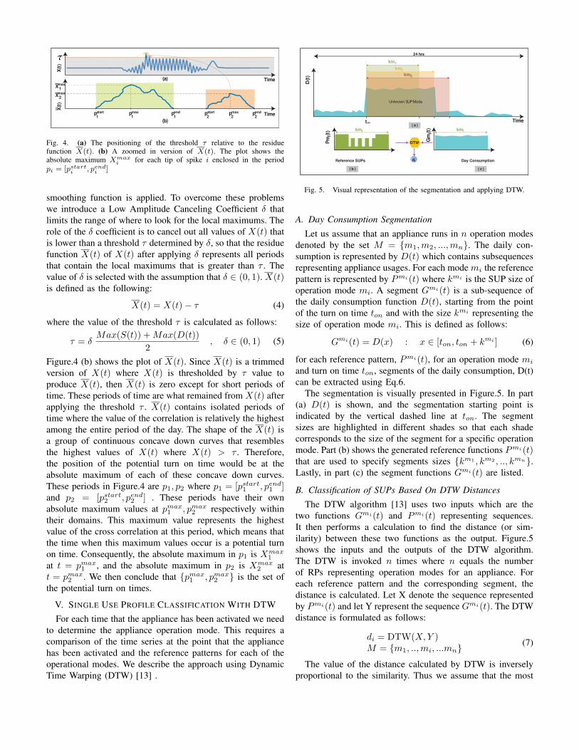
Fig. 4. (a) The positioning of the threshold τ relative to the residuefunction X(t). (b) A zoomed in version of X(t). The plot shows theabsolute maximum Xmax

i for each tip of spike i enclosed in the periodpi = [pstarti , pend

i ]

smoothing function is applied. To overcome these problemswe introduce a Low Amplitude Canceling Coefficient δ thatlimits the range of where to look for the local maximums. Therole of the δ coefficient is to cancel out all values of X(t) thatis lower than a threshold τ determined by δ, so that the residuefunction X(t) of X(t) after applying δ represents all periodsthat contain the local maximums that is greater than τ . Thevalue of δ is selected with the assumption that δ ∈ (0, 1). X(t)is defined as the following:

X(t) = X(t)− τ (4)

where the value of the threshold τ is calculated as follows:

τ = δMax(S(t)) +Max(D(t))

2, δ ∈ (0, 1) (5)

Figure.4 (b) shows the plot of X(t). Since X(t) is a trimmedversion of X(t) where X(t) is thresholded by τ value toproduce X(t), then X(t) is zero except for short periods oftime. These periods of time are what remained from X(t) afterapplying the threshold τ . X(t) contains isolated periods oftime where the value of the correlation is relatively the highestamong the entire period of the day. The shape of the X(t) isa group of continuous concave down curves that resemblesthe highest values of X(t) where X(t) > τ . Therefore,the position of the potential turn on time would be at theabsolute maximum of each of these concave down curves.These periods in Figure.4 are p1, p2 where p1 = [pstart1 , pend1 ]and p2 = [pstart2 , pend2 ] . These periods have their ownabsolute maximum values at pmax

1 , pmax2 respectively within

their domains. This maximum value represents the highestvalue of the cross correlation at this period, which means thatthe time when this maximum values occur is a potential turnon time. Consequently, the absolute maximum in p1 is Xmax

1

at t = pmax1 , and the absolute maximum in p2 is Xmax

2 att = pmax

2 . We then conclude that {pmax1 , pmax

2 } is the set ofthe potential turn on times.

V. SINGLE USE PROFILE CLASSIFICATION WITH DTWFor each time that the appliance has been activated we need

to determine the appliance operation mode. This requires acomparison of the time series at the point that the appliancehas been activated and the reference patterns for each of theoperational modes. We describe the approach using DynamicTime Warping (DTW) [13] .

Day Consumption

Time

D(t

)

Pm

(t)

i

km

km

km

24 hrs

( a )

( b ) ( c )

ton

DTW

Reference SUPs d

Unknown SUP Mode

kmikm

i

i

Gm

(t)

i

3

2

1

Fig. 5. Visual representation of the segmentation and applying DTW.

A. Day Consumption Segmentation

Let us assume that an appliance runs in n operation modesdenoted by the set M = {m1,m2, ...,mn}. The daily con-sumption is represented by D(t) which contains subsequencesrepresenting appliance usages. For each mode mi the referencepattern is represented by Pmi(t) where kmi is the SUP size ofoperation mode mi. A segment Gmi(t) is a sub-sequence ofthe daily consumption function D(t), starting from the pointof the turn on time ton and with the size kmi representing thesize of operation mode mi. This is defined as follows:

Gmi(t) = D(x) : x ∈ [ton, ton + kmi ] (6)

for each reference pattern, Pmi(t), for an operation mode mi

and turn on time ton, segments of the daily consumption, D(t)can be extracted using Eq.6.

The segmentation is visually presented in Figure.5. In part(a) D(t) is shown, and the segmentation starting point isindicated by the vertical dashed line at ton. The segmentsizes are highlighted in different shades so that each shadecorresponds to the size of the segment for a specific operationmode. Part (b) shows the generated reference functions Pmi(t)that are used to specify segments sizes {km1 , km2 , .., kmn}.Lastly, in part (c) the segment functions Gmi(t) are listed.

B. Classification of SUPs Based On DTW Distances

The DTW algorithm [13] uses two inputs which are thetwo functions Gmi(t) and Pmi(t) representing sequences.It then performs a calculation to find the distance (or sim-ilarity) between these two functions as the output. Figure.5shows the inputs and the outputs of the DTW algorithm.The DTW is invoked n times where n equals the numberof RPs representing operation modes for an appliance. Foreach reference pattern and the corresponding segment, thedistance is calculated. Let X denote the sequence representedby Pmi(t) and let Y represent the sequence Gmi(t). The DTWdistance is formulated as follows:

di = DTW(X,Y )M = {m1, ..,mi, ...mn}

(7)

The value of the distance calculated by DTW is inverselyproportional to the similarity. Thus we assume that the most

0 200 400 600 800 1000 1200 1400Reference Pattern Size n (Samples)

0

1

2800

10001200

Num

ber o

f d

etec

ted

SUPs Dishwasher

Clothes washerClothes dryer

Fig. 6. The impact of changing the reference pattern size n on the numberof detected SUPs in the day consumption date for a dishwasher, a clotheswasher, and a clothes dryer.

similar reference pattern is the reference pattern with theminimum distance. This means that the mode m∗ with theminimum distance d∗ that is the operation mode of theappliance at the SUP detected at ton as:

d∗ = min(d1, d2, ..., dmi)

VI. POWER CONSUMPTION SIMULATION

It is necessary to create simulated data when it is impracticalto obtain real data that there is an insufficient amount of certaintype data such as our case when there is no such PCD thatcontains disaggregated data with different operation modes foran appliance. Our Power Consumption Simulator (PCS) mainpurpose is to simulate appliances consumption with differentoperation modes by generating daily usage data that has SUPsfor different operation modes.

PCS has three configuration parameters: Turn On Timeton, Household Usage Intensity (Ih), and SUP RepresentationObject (SUPRO). ton refers to the time when an appliance,a, is activated by the user during the day. We use the InverseTransform Sampling (ITS) [9] method to sample values of tonProbability Density Function (PDF) that is extracted from aPCD. Household Usage Intensity (Iah) refers to the distributionof operation modes that a household, h, uses for an appliance,a, over time. We assume that the selection of an applianceoperation mode for a household is based on a multinomialdistribution function. The frequencies of this distribution is20% for operation modes used fewer number of times and 60%for the operation modes used more. Single Usage Profile Representation Object (SUPRO) is a representational model of aSUP for an appliance in a particular operation mode. It definesCycles which are periods of time when the power consumptionis stable around fixed wattage. Each cycle is defined by theduration and the wattage it has. Also, SUPRO defines Phaseswhich are groups of cycles in certain repetition bounded bylower and upper bounds.

VII. RESULTS AND DISCUSSION

This section discusses the results of applying SUP detectiontechnique using XCORR and SUP classification using DTWon a test data.

A. Single Usage Profile Detection

The evaluation metric we use is the number of detectedSUPs for certain appliance. This corresponds to the numberof reported turn on times for certain appliance by the SUP

Fig. 7. The precision, recall and F1-score for each operation mode usingDTW.

detection algorithm. We assume that a single SUP presentsdaily for an appliance. We generated reference patterns ofdifferent sizes n based on a SUP generated with a randomlyselected operation mode (see VI). We assume that the valueof the Low Amplitude Canceling Coefficient δ is equal to 90and the sampling frequency used is fs = 1Hz.

Figure.6 shows the results for a dishwasher, a clotheswasher, and a clothes dryer. For the dishwasher, it shows avery large number of detected SUPs found in the day whenn is between 50 and 400. This is because of the shape ofthe SUP of the dishwasher. When the reference pattern sizeis between 50 and 400, there is a high number of SUPsdetected despite the existence of only one SUP. However,the number of detected SUP settles down to one when thereference pattern size typically increases within the range 400and 1400 samples. When the reference pattern size exceeds1400 samples, the number of detected SUPs is zero. For theclothes washer. When the reference pattern size is between100 and 1100 samples, the number of detected potential SUPsis always one. That is probably because the repetition in thewasher consumption curve is minimal, thus, a unique one highvalue of cross correlation in every test. For the clothes dryer,it shows that the value of n that gives best results is when n isbetween 600 and 1100 samples where it shows the number ofdetected SUPs equals to one. Nevertheless, the results showsome choppiness in the number of detected SUPs. This is acommon problem for all appliances. It is most likely due to thevariations in cycles duration where cycle duration is generatedwith variation factor that affects XCORR by reducing theoverlapping between the cycles in the reference pattern andthe detected SUP.

The number of matching SUPs is higher for shorter refer-ence pattern than a longer reference pattern. This is becausethere is higher chance that small reference pattern occursmore frequently within the consumption function than a longerreference pattern. The reason is that a SUP has repetitions ofcycles that have similar shape. This shape could be similar tothe reference pattern. This leads to reporting multiple potentialSUPs even where is only one SUP. Thus, as the size ofreference pattern decreases, the probability of reporting theserepetitions within a SUP is higher. Therefore, the accuracyincreases as the reference pattern size increases.

B. Single Usage Profile Classification

To test the performance of the DTW classifier, we generatepower consumption data for three different households usingthe simulator. These datasets are distinct in appliance usagein terms of Ih. We assume that for each appliance, there arethree different levels of Ih: High, Medium, and Low.

We use three metrics to measure the performance of theclassifiers we use. The metrics are the following: Precision,Recall, F1-score. Figure.7 shows that for the DTW the metricsvalues are averaged around 82% for the light and heavy op-eration modes. Otherwise, the metrics value is approximately79%.

The breakdown of the operation modes performance foreach appliance is shown in Figure.8. The chart is dividedinto three main lanes, each lane corresponds to an appliance.Within each lane, it shows the different metric values for DTWclassification results over the operation modes. Generally, thechart shows higher performance for the light and heavy oper-ation modes. In the clothes washer lane, there is a variation inthe metrics values from operation mode to another. However,in the clothes dryer and the dishwasher lanes,it shows higherperformance for heavy and light modes more noticeably in theclothes dryer.

VIII. CONCLUSION AND FUTURE WORK

Our work is focused on providing techniques built on topof residential power consumption for certain appliances. Thesetechniques serve as the foundation that can built upon to bettersupport DR. We analyzed PCD [7] by applying statisticalanalysis to find out statistical distributions about consumptionfor the households in the dataset. Furthermore we used someof the analysis in the literature [12] to understand operationmodes for appliances and extract their characteristics. A sim-ulation engine then processes the statistical models resultedfrom the data analysis and generates power consumptiondata to simulate households use their appliances in differentoperation modes. This simulated data is used to test ourmodels. An SUP detection algorithm is proposed using crosscorrelation between reference patterns and daily usage datato detect the activation times of appliances. These activationtimes are used by the recognition algorithm (DTW) to classifySUPs into their operation modes. A future improvement tothe current work is to utilize other versions of DTW such asAWrap [10] for sparse time series that is faster the originalDTW. This provides opportunities to apply this work on onlinepower consumption data streams collected by smart meters andsensors.

REFERENCES

[1] Jose M Alcala, Jesus Urena, and Alvaro Hernandez. Event-baseddetector for non-intrusive load monitoring based on the hilbert transform.In Proceedings of the 2014 IEEE Emerging Technology and FactoryAutomation (ETFA), pages 1–4. IEEE, 2014.

[2] Leen De Baets, Joeri Ruyssinck, Dirk Deschrijver, and Tom Dhaene.Event detection in nilm using cepstrum smoothing. In 3rd InternationalWorkshop on Non-Intrusive Load Monitoring, pages 1–4, 2016.

Heavy Light Medium Heavy Light Medium Heavy Light Medium

1.0

F1 S

core

0.5

1.0

Prec

isio

n

0.5

1.0

Reca

ll

0.5

Appliance / Algor ithm / M deo

Clothes Dryer Clothes W as her Dis hW as her

Fig. 8. The breakdown of the operation modes performance for each applianceusing DTW and KNN algorithms.

[3] Sebastian Golz. Does feedback usage lead to electricity savings? analysisof goals for usage, feedback seeking, and consumption behavior. EnergyEfficiency, 10(6):1453–1473, 2017.

[4] Jing Liao, Georgia Elafoudi, Lina Stankovic, and Vladimir Stankovic.Power disaggregation for low-sampling rate data. In 2nd InternationalNon-intrusive Appliance Load Monitoring Workshop, Austin, TX, 2014.

[5] Bo Liu, Wenpeng Luan, and Yixin Yu. Dynamic time warping basednon-intrusive load transient identification. Applied energy, 195:634–645,2017.

[6] J. M. G. Lpez, E. Pouresmaeil, C. A. Caizares, K. Bhattacharya,A. Mosaddegh, and B. V. Solanki. Smart residential load simulatorfor energy management in smart grids. IEEE Transactions on IndustrialElectronics, 66(2):1443–1452, Feb 2019.

[7] Stephen Makonin, Z. Jane Wang, and Chris Tumpach. RAE: TheRainforest Automation Energy Dataset for Smart Grid Meter DataAnalysis. pages 1–9, 2017.

[8] William Menke and Joshua Menke. Ch9 - detecting correlations amongdata. In William Menke and Joshua Menke, editors, Environmental DataAnalysis with Matlab (Second Edition), pages 187 – 221. AcademicPress, second edition edition, 2016.

[9] F.P. Miller, A.F. Vandome, and M.B. John. Inverse Transform Sampling.VDM Publishing, 2010.

[10] Abdullah Mueen, Nikan Chavoshi, Noor Abu-El-Rub, HosseinHamooni, Amanda Minnich, and Jonathan MacCarthy. Speeding updynamic time warping distance for sparse time series data. Knowledgeand Information Systems, 54(1):237–263, Jan 2018.

[11] Natural Resources Canada. Energy facts, 2019. [Online athttps://bit.ly/2WAgjq5; accessed 1-November-2019].

[12] Manisa Pipattanasomporn, Murat Kuzlu, Saifur Rahman, and YonaelTeklu. Load Profiles of Selected Major Household Appliances and TheirDemand Response Opportunities. IEEE Transactions on Smart Grid,5(2):742–750, mar 2014.

[13] Chotirat Ann Ratanamahatana and Eamonn Keogh. Everything youknow about dynamic time warping is wrong. In Third workshop onmining temporal and sequential data, volume 32. Citeseer, 2004.

[14] Luis Rueda, Alben Cardenas, Sousso Kelouwani, and Kodjo Agbossou.Transient event classification based on wavelet neuronal network andmatched filters. In IECON 2018-44th Annual Conference of the IEEEIndustrial Electronics Society, pages 832–837. IEEE, 2018.

[15] Guoming Tang, Kui Wu, Jingsheng Lei, and Weidong Xiao. Themeter tells you are at home! non-intrusive occupancy detection via loadcurve data. In 2015 IEEE International Conference on Smart GridCommunications (SmartGridComm), pages 897–902. IEEE, 2015.

[16] The International Energy Agency. Demand response: Tracking cleanenergy progress, 2019. [Online at https://bit.ly/2PrWcZJ; accessed 27-October-2019].

[17] U.S. Energy Information Administration (EIA). Demand responsesaves electricity during times of high demand, 2016. [Online athttps://bit.ly/2MTfuW4; accessed 27-October-2019].

[18] Huijuan Wang and Wenrong Yang. An iterative load disaggregationapproach based on appliance consumption pattern. Applied Sciences,8(4):542, 2018.

[19] Yi Wang, Qixin Chen, Tao Hong, and Chongqing Kang. Review of smartmeter data analytics: Applications, methodologies, and challenges. IEEETransactions on Smart Grid, 10(3):3125–3148, 2018.