Demand Side Energy Management via Multiagent Coordination inConsumer Cooperatives

Andreas Veit? Ying Xu† Ronghuo Zheng† Nilanjan Chakraborty‡ Katia Sycara‡

?Karlsruhe Institute of Technology †Tepper School of BusinessKaiserstrasse 12 Carnegie Mellon University

76131 Karlsruhe, Germany. Pittsburgh, PA 15213

‡Robotics Institute, School of Computer ScienceCarnegie Mellon University

Pittsburgh, PA 15213

Abstract

A key challenge in creating a sustainable and energy-efficient society is to make consumer demandadaptive to the supply of energy, especially to renewable supply. In this paper, we propose a partially-centralized organization of consumers (or agents), namely, a consumer cooperative for purchasing elec-tricity from the market. We propose a novel multiagent coordination algorithm, to shape the energyconsumption of the cooperative. In the cooperative, a central coordinator buys the electricity for thewhole group and consumers make their own consumption decisions, based on their private consumptionconstraints and preferences. To coordinate individual consumers under incomplete information, we pro-pose an iterative algorithm, in which a virtual price signal is sent by the coordinator to induce consumersto shift their demands when required. This algorithm provably converges to the central optimal solutionand minimizes the electric energy cost of the cooperative. Additionally, we perform simulations basedon real world consumption data to characterize (a) the convergence properties of our algorithm and (b)understand the effect of different parameters that characterize the electricity consumption profile on thepotential cost reduction through coordination by our algorithm. The results show that as the participants’flexibility of shifting their demands increases, cost reduction increases. We also observe that the cost re-duction is not very sensitive to the variation in consumption patterns of the consumers (e.g., whether theconsumers use more electricity during the evening or during the day). Finally, our simulations indicatethat the convergence time of the algorithm scales linearly with the agent population size.

1 Introduction

According to the US Department of Energy, the creation of a sustainable and energy-efficient society is oneof the greatest challenges of this century, as traditional non-renewable sources of energy are depleting andadverse effects of carbon emissions are being felt (DOE, 2003). Two key issues in creating a sustainableand energy-efficient society are reducing peak energy demands and increasing the penetration of renewableenergy sources. In order to achieve a reliable operation of the electricity distribution system, supply andthe load have to be balanced within a tight tolerance in real time. One way, which is most commonly used,to achieve the demand supply balance is to supply all the required demand whenever it occurs. However,

1

attempting to achieve demand supply balance by adjusting only the supply side leads to the use of flexible(usually diesel operated) power plants that can be expensive, inefficient, and emit large amount of carbon.An alternative to adjusting the supply side only is to also adjust the demand of the consumers, so thatflexible power plants required to operate for meeting peak demands are used as little as possible (Palensky &Dietrich, 2011). Managing the demand side becomes more critical when the uncertainty in the energy supplyincreases as is the case with increasing penetration of renewable energy in the electricity market (Medina,Muller, & Roytelman, 2010). In order to adjust consumer demands, various demand response programshave been introduced. Demand Response (DR) can be defined as ”the changes in electricity consumptionby end users from their normal consumption patterns in response to changes in the price of electricity overtime” (Albadi & El-Saadany, 2007).

Several different forms of demand response programs have been developed (for an overview see (Albadi& El-Saadany, 2007)). The first type of programs are incentive based programs (IBP), where customersreceive payments for their participation in the programs. A typical example of an IBP are Direct LoadControl (DLC) programs, in which utilities have the ability to remotely control the power consumption ofconsumers’ appliances by switching them on/off. In small scale pilot studies, DLC has been successful inreducing peak energy consumption. However, the biggest drawback of DLC is that consumers may not becomfortable with utility companies having direct control over their appliances (Rahimi & Ipakchi, 2010;Medina et al., 2010).

The second type of programs are price based programs (PBP), which are based on variable pricing rates,so that energy rates follow the real cost of electricity. The objective of this indirect method is to controlthe overall demand by incentivizing consumers to flatten the demand curve by shifting energy from peakto off-peak times. The basic example of PBP are TOU programs, in which the rate during peak times ishigher than the rate during other off-peak times. Recent technological advances in smart meters and smartappliances have enabled direct and real time participation (RTP) of an individual consumer in the energymarket through the use of software agents. This allows price based systems with hourly prices dependingon the actual cost of generation. A key feature of RTP programs is that each customer communicates withthe utility companies individually. However, there are two key problems in realizing this potential. First,despite the presence of small pilot programs, the end users are usually not of sufficient size for the utilities tobe considered for demand response services. Second, if end users participate in the market directly, withoutcontrol by the utility companies, the stability of the system may be compromised, due to uncontrolleddistributed interactions (Ramchurn, Vytelingum, Rogers, & Jennings, 2012).

In (Mohsenian-Rad, Wong, Jatskevich, Schober, & Leon-Garcia, 2010) it is argued that a good de-mand side management program should focus on controlling the aggregate load (which is also importantfor economic load dispatching (Wood & Wollenberg, 1996)) of a group of consumers instead of individualconsumers. Therefore, in this paper the problem of coordinating a group of consumers called consumercooperatives is introduced and studied. A consumer cooperative allows partial centralization of consumersrepresented by a group coordinator (mediator) agent, who purchases electricity from utilities or the marketon their behalf. Such consumer configurations can potentially increase energy efficiency via aggregation ofdemand to reduce peak power consumption, and direct participation in the energy markets. The coordinatoris neither a market maker nor a traditional demand response aggregator (Jellings & Chamberlin, 1993), sinceit does not set energy prices or aims to incur profits by selling to the market. Rather, its role is akin to asocial planner’s, in the sense that it manages the demand of its associated consumer group for cost effectiveelectricity allocation. It has to ensure that the demand goals and constraints of the group members (con-sumers) are fulfilled, while also enabling to flatten out peak demands for the group. The consumers espousethe goals of the group, but they are not willing to completely disclose their demand goals and constraints to

2

either other firms or the coordinator. Moreover, the members autonomously decide how to shift their loadsto help the group flatten peak demands. Real world consumer groups coordinated in the above manner canbe formed naturally in many application scenarios, especially when they are geographically co-located, e.g.,industrial parks/technology parks, commercial estates or large residential complexes.

Consumer cooperatives offer advantages to both energy utility companies and consumers. From theutility’s perspective, the consumer groups are large enough to be useful in demand response programs andhave more predictable demand shifts compared to individual consumers. The partially centralized modeloffers several advantages to the stakeholders: For individual consumers, participation in such energy groupsallows them to retain control of their own appliances. In addition, the consumers can obtain electricity atbetter prices than they would have if they had purchased electricity individually. The price advantage is dueto three reasons. First, the group’s size is of importance, since the mediated participation of the consumergroup in the market allows the group to enter into more flexible purchase contracts, so that the price paid bythe consumers reflects the actual cost of production more accurately (which is not the case in current longterm fixed contract structures (Kirschen, 2003)). Second, by buying collectively, the group can benefit fromvolume discounts. The situation here is analogous to group insurance programs in companies. Third, innegotiated electricity contracts, the price usually consists of two components, one coming from the actualenergy production cost and the other as a premium against volatility in the energy demand and/or supply.Buying as a group can help in reducing the premium against volatility, provided the demands of the groupmembers are coordinated, so that their total demand is more stable and lower during demand peaks. Thus,in this paper, we study the problem of coordinating the electricity demand of agents who are purchasingelectricity as a consumer cooperative.

The objective of this coordination is to minimize the cost function of the total cost of procuring elec-tricity. The technical challenge in designing a coordinated demand management for a consumer cooperativeis the fact that the central coordinator does not know the constraints of the individual consumers, and thuscannot compute the optimal demand schedule on its own. Furthermore, the actual cost of electricity con-sumption will depend on the aggregate consumption profile of all agents. However, the agents may notwant to share their consumption patterns or consumption constraints with other agents. Therefore, in thispaper, an algorithm is designed that enables the central agent to coordinate the consumers to achieve theoptimal centralized consumption load, while the individual agents retain their private knowledge about theirconsumption constraints.

We first consider the simple but practically relevant problem with a planning horizon of only two timeslots with different electricity prices, where agents have demand constraints that have to be satisfied, but theydo not have any cost for shifting demands between different time slots. This will be called the basic setting.We design a simple iterative algorithm, where in each iteration the coordinator computes virtual price signalsand sends them to the consumers, who then compute their optimal consumption profiles based on this pricesignal and send it back to the coordinator. This will be called the basic coordination algorithm. We showthat in the problem setting with only two time slots and no cost for shifting demand, this iterative algorithmconverges to the optimal schedule. We then consider settings with a planning horizon of more than two timeslots with different electricity prices and with individual costs for the agents to shift demand. This will becalled the general setting. Since the basic algorithm does not guarantee the optimal solution for generalsetting, we design an iterative algorithm that includes an additional phase. This general algorithm first runsthe basic algorithm until it converges and then the additional phase if necessary. In that additional phase, ineach iteration, the agents compute their marginal valuation for their electricity demand in addition to theiroptimal consumption profiles and send them back to the coordinator. The coordinator uses the additionalinformation to adapt the virtual price signals. We show that this general iterative algorithm converges to the

3

optimal schedule in the general setting. These provably optimal demand scheduling algorithms for consumercooperatives are the primary contribution of this paper. We also conduct simulation studies to characterize(a) the convergence properties of our algorithm and (b) understand the effect of different parameters thatcharacterize the electricity consumption profile on the potential cost reduction through coordination bythe algorithm. The results show that as the participants’ flexibility of shifting their demands increases,cost reduction increases. We also observe that the cost reduction is not very sensitive to the variation inconsumption patterns of the consumers (e.g., whether the consumers use more electricity during the eveningor during the day). Finally, our simulations indicate that the convergence time of the algorithm scaleslinearly with the agent population size. A preliminary version of this work appeared in (Veit, Xu, Zheng,Chakraborty, & Sycara, 2013).

This paper is organized as follows: In Section 2 we give an overview of the related work and pointout the differences to the approach in this paper. In Section 3 we formulate the cost optimization problemof the consumer cooperative. Then in Section 4 we introduce the demand scheduling algorithms for theconsumer cooperative. In particular, in Section 4.1 we introduce the basic iterative algorithm for which weprove in Section 4.2 that it converges to the optimal solution in basic settings with only two time slots andno cost of shifting demand. In Section 5 we introduce the general iterative algorithm for which we provein Section 5.3 that it converges to the optimal solution in general settings. Subsequently, in Section 6 weevaluate the coordination algorithms using simulations based on ral world consumption data. In particular,in Section 6.1 we describe the data sets used for the simulations and explain the parameterization of thesimulation scenarios. In Section 6.2 we discuss the results of the simulations, regarding the potential costreduction through coordination as well as the convergence properties of the algorithm. Finally in Section 7we summarize the main contributions of this paper and give an outlook on future work.

2 Related Work

The literature on demand management and demand response is extensive. As mentioned in the introduction,the demand response programs vary from classical direct load control (DLC) to price based programs withreal time prices (RTP). In this paper we introduce an algorithm that uses variable price signals to coordi-nate the energy consumption of a consumer cooperative. Therefore we restrict this discussion to demandmanagement using variable price signals.

The initial pricing schemes utilizing variable price signals in order to influence consumer demand usedprices for electricity that varied according to the time of the day or day of the year. These traditionaltime of use (TOU) pricing schemes penalize certain periods of time with a higher electricity price, so thatcustomers respond to these signals by adjusting their consumption to reduce their own cost. Thereby, theelectricity price is set to be high at times having typically high consumption so that demand during peakload times can be reduced. However, TOU does not necessarily reduce the overall energy demand, but onlythe consumption patterns are influenced (Rahimi & Ipakchi, 2010; Kirschen, 2003; Medina et al., 2010;Albadi & El-Saadany, 2007; Palensky & Dietrich, 2011). Most of the literature looking at price baseddemand response programs considers the case of deterministic prices, in which the electricity prices of alltime slots are known before consumption. This case can be applied to all long-term contract markets andday-ahead markets if the planning horizon is sufficiently short (see (Vytelingum, Ramchurn, Rogers, &Jennings, 2010) and (Ramchurn, Vytelingum, Rogers, & Jennings, 2011)). Known electricity prices areused so that a central manager can deliver the information to consumers to incentivize consumers to shiftdemand to times with low-prices.

Current literature on demand shaping mostly operates in the paradigm that it is desirable to have a

4

system where the consumer can set its preferences and constraints about the timing of the operation ofthe appliances (or loads), and have an automated (or autonomous) system that ensures the electricity costis minimized while the user preferences are met. It is (implicitly or explicitly) assumed that the utilitycompanies can send a price signal to software agents at those systems (or smart meters) that respond to thisprice and schedule the appliances for the future.

The different approaches for demand scheduling proposed in the literature differ in some central char-acteristics. First they differ in the objective of the demand scheduling and secondly they differ in the level atwhich the problem is solved. Different objectives include minimizing the cost of a single consumer, mini-mizing the total cost of power generation, reducing the peak-to-average ratio in demand and optimizing gridstability. The different levels at which the problem has been studied include the level of the single user, themarket maker, as well as the grid operator.

When the demand scheduling problem is studied at the grid operator level, the grid stability (not theenergy cost) is the main objective. In particular, objectives include the minimization of power flow fluc-tuations (Tanaka, Uchida, Ogimi, Goya, Yona, Senjy, Funabashi, & Kim, 2011), integration of greenenergy (Wu, Mohsenian-Rad, & Huang, 2012) and the minimization of power losses and voltage devia-tions (Clement-Nyns, Haesen, & Driesen, 2010).

Most work on demand scheduling focuses at the level of the end users. An important characteristic ofthe end user is that it cannot influence the electricity prices, i.e., the end user is a price taker. In demandscheduling for end users the usual objective is to minimize the cost of electricity consumption of a residentialor commercial end user by optimally scheduling the demand. However, the studies differ in some key char-acteristics. Differences include the particular problem they solve, the assumption on the knowledge aboutthe prices and demand and whether an optimal solution to the optimization problem is guaranteed. In (Chu& Jong, 2008) the authors assume known electricity prices and demand for their cost optimization. Howeverthey restrict the considered loads to air conditioning systems and in contrast to this paper the authors focuson load shedding and not load shifting. The authors in (Pedrasa, Spooner, & MacGill, 2010) also assumeknown prices and demand, but for their optimization they use Particle Swarm Optimization. In (Philpott &Pettersen, 2006) and (Samadi, Mohsenian-Rad, Wong, & Schober, 2013) the prices for electricity are known, but no central knowledge of the demand is assumed, only an estimate. In (Philpott & Pettersen, 2006) theauthors study how to optimally bid in the day ahead electricity market, if the actual demand is uncertain andthe difference to the bid has to be bought from the real time market. In (Samadi et al., 2013) the authorsformulate an optimization problem for the real time residential load management that only requires somestatistical estimates of the future load demand.

The next studies focus on a setting where the demand is assumed to be known but there is price uncer-tainty. In (Conejo, Morales, & Baringo, 2010) the authors present a procedure to adjust the hourly load levelof a household in response to real-time electricity prices, where only the price for the next hour is known.In (Kim & Poor, 2011) the scheduler only has statistical knowledge about the future prices and the schedul-ing problem is thus modeled as a Markov decision process. In (Mohsenian-Rad & Leon-Garcia, 2010) theenergy consumption of a household is also scheduled in response to time-varying prices. In addition theauthors claim that the use of an inclining block rate as pricing scheme can prevent load synchronization.However they only consider one consumer that has perfect knowledge about the load of all appliances.

In practice, it may be difficult for utility companies or grid operators to deal with individual end usersin such demand response programs. The demand shift of an individual end user might be too small inmagnitude compared to the aggregated necessary shift. Thus, it is unclear whether such a scheme will inducea shift of sufficient size. Moreover there have been concerns voiced that the stability of the system may becompromised with such uncontrolled distributed interactions (Kirschen, 2003). In our work the demand

5

scheduling problem is solved at the level of a consumer cooperative where the objective is to minimizethe electricity procurement cost for the cooperative. The demand constraints and preferences are privateknowledge to the consumers and not known to the coordinator. The cooperative is also a price taker, becausethe cooperative buys the electricity from a utility company. From the utility’s perspective, the consumercooperative is large enough to be useful in demand response programs.

There are also studies in the extant literature that focus on the demand scheduling at the level of themarket maker. In contrast to the previous approaches this means that the coordinator can set the prices forelectricity. The objective in these studies is mostly to minimize the total cost of power generation. In (Diet-rich, Latorre, Olmos, & Ramos, 2012) an electric system with high wind penetration is modeled in order tocompare different demand response programs. They compare demand shifting vs. peak shaving as well ascentralized vs. decentralized approaches. They conclude that the centralized approach reaches higher over-all cost savings, but has the disadvantage that central knowledge of consumers’ constraints and preferencesis necessary. The authors in (Parvania & Fotuhi-Firuzabad, 2010) present a stochastic model to schedulereserves provided by demand response in the wholesale electricity markets. In order to create consumersthat are of sufficient size for demand response programs they introduce demand response providers that ag-gregate end consumers. Some other studies use game theoretic approaches to model the consumer behavior.In (Atzeni, Ordonez, Scutari, Palomar, & Fonollosa, 2013) the authors formulate the day-ahead grid opti-mization problem, whereby each user on the demand-side minimizes its individual cost. In (Vytelingum,Voice, Ramchurn, Rogers, & Jennings, 2011) the authors look at the challenges of the adoption of micro-storage devices for the energy system. The authors characterize the competition equilibrium of the amountof storage that will be adopted by the population. In (Wu, Mohsenian-Rad, Huang, & Wang, 2011) theauthors propose a demand side management method to tackle the temporal variations in wind power gen-eration. Using game theory, they analyze the interactions among users to efficiently utilize the availablerenewable and conventional energy. Some studies consider further objectives. In (Nguyen, Song, & Han,2012) the authors focus on reducing the peak-to-average ratio (PAR) of consumption. In order to reduce thePAR, users request their energy demands to an energy provider, who dynamically updates the energy pricesbased on the loads of the users. Another objective is used by the authors in (Baharlouei, Hashemi, Narimani,& Mohsenian-Rad, 2013). They develop an electricity billing mechanism that focuses on both reducing costand ensuring fairness. A key feature of many of those works is that the agents communicate directly with theutilities and hence, the focus is on controlling the overall load by interacting directly with each consumer.There is no interaction among the consumers. However (Ramchurn et al., 2011) mentions that such variableprice signals can only work for a small number of houses whereas in a large scale with many customersthere is a possibility it may not reduce demand peak and even cause instabilities like herding phenomenon.Thereby agents synchronize their load, because they move their consumptions towards the low price timesand thus cause a spike in demand, leading to increasing energy cost (Ramchurn et al., 2012). Althoughsome heuristics have been proposed to address this issue, there is no algorithm with provable guarantees tosolve this problem. In order to stabilize the system in (Voice, Vytelingum, Ramchurn, Rogers, & Jennings,2011) agents are charged an additional fee based on how much they change their storage profile from oneperiod to the next. In (Ramchurn et al., 2011) the authors introduce an adaptive mechanism controlling therate and frequency at which the agents are allowed to adapt their loads and to readjust their heating profile.In (Vytelingum et al., 2010) a compensation signal is sent to the agents providing an estimate of how muchthey should aim to change their behavior.

Another approach is proposed by (Mohsenian-Rad et al., 2010) focusing on a utility or a generator con-trolling the load of a group of consumers. The authors accomplish this by allowing the individual consumersto interact with one another. The problem is formulated in a game-theoretic framework and the consumers

6

coordinate in an iterative manner and exchange their demand profiles (but not their consumption constraintswith each other). In our paper, consumers interact as a coordinated group with the utility in order to preventload synchronization, but the consumer architecture is different. The consumers form a cooperative with acentral coordinator and the agents do not share their consumption profiles with other agents.

3 Problem Formulation

In this paper we consider a setting in which a central coordinator purchases electricity from a supplier tosupport the demands of a consumer group. Figure 1a shows an example of such a consumer group. Thegroup consists of several commercial consumers that use one central coordinator to purchase the necessaryelectricity from a supplier or from the electricity market. The flow of money is illustrated by the green dottedarrows. The yellow dashed arrows show the flow of electricity. For the coordination there is an exchangeof information between the coordinator and the individual agents. This flow of information is illustrated bythe blue arrows. We assume that the price of electricity is known over the whole planning horizon. This istrue when the agent group has a long-term electricity contract (say yearly) and the agents planning horizonis shorter (say 1 day). The contract is not a flat-rate contract, since in this case there would be no economicincentive for the agents to shift their demands.

We consider the consumer group to consist of N members with the planning period divided into Mdiscrete time slots. The amount of discrete time slots depends on the market price structure, which can bedifferent in practice, based on the utility companies. Figure 1b shows the logical schema of such a consumergroup. The Figure illustrates how the coordinator aggregates the demands of the N agents of the planninghorizon of M discrete time slots. Note that M = 2 for time-of-use pricing with different prices during dayand night, whereas M = 24 in an hourly pricing scheme. Let R be an N ×M matrix where each row of thematrix, ri is the electricity demand of the agent i, i ∈ {1, 2, . . . , N}. We call ri the demand profile of agenti. Each entry rij is the electricity demand of agent i for time slot j. The total aggregated demand in timeslot j is ρj =

∑Ni=1 rij . The average market price of a unit of electricity for the consumer group at time slot

j is defined as pj(ρj).We assume a typical market price function where the prices are different in each time slot and the price

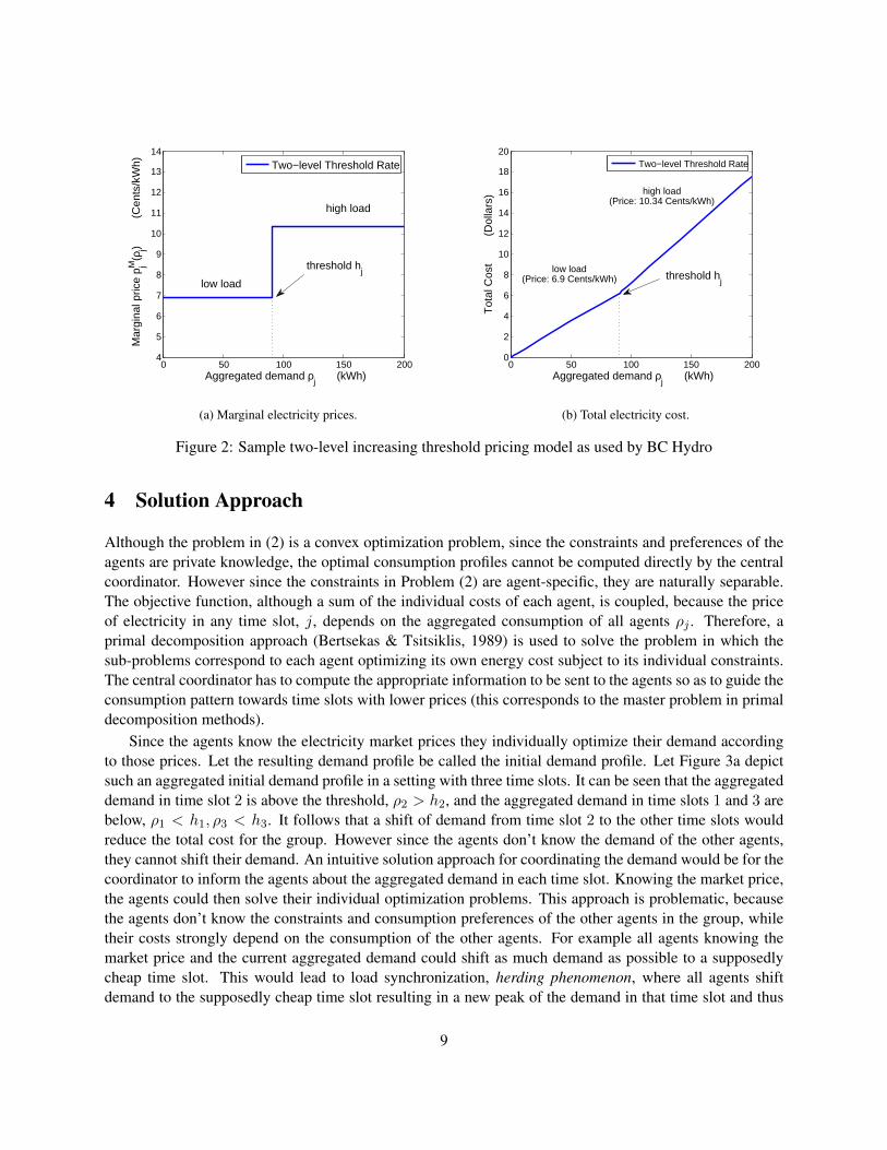
has a threshold structure. This means that the marginal electricity prices differ among different consumptionlevels. For each time slot, every unit of electricity consumed below a specified threshold is charged at alower price, while any additional unit exceeding that threshold is charged at a higher price. This is anexample of a non-flat electricity pricing rate, which has also been called a ”two-level inclining block rate”by (Mohsenian-Rad & Leon-Garcia, 2010). Thus, the marginal electricity price in a time slot, denoted bypmj (ρj), is a non-decreasing function of the total demand. The marginal price at a given consumption level

is the payment increment (decrement) for adding (reducing) one unit of electricity. Figure (2a) shows anexample of a two-level increasing threshold pricing model adopted from BC Hydro.1 The marginal price

of a two-level threshold structure can formally be written as follows: pmj (ρj) =

{pHj ρj > hj

pLj ρj ≤ hjwith

pHj > pLj , where hj is the threshold for consumption in time slot j. We further assume that the high pricein any time slot is greater than the low price in any other time slot, i.e., pHj > pLk , ∀j, k. Let for the furtheranalysis x+ = max {0, x} and x− = min {0, x}. The total energy cost for time slot j is thus the integralof the marginal prices. Figure (2b) shows the total electricity cost for the aggregated demand based on the

1BC Hydro is a Canadian utility company. This pricing model is obtained from www.bchydro.com.

7

money

electricity

coordinationinformation

(a) Example setup of real world cooperative.

Coordinator

N agents . . .

Supplier

. . .M time slots

electricity contract

(b) Logical schema of a cooperative.

Figure 1: System overview of the architecture as considered in this paper including the cooperative andsupply.

two-level level threshold pricing model. The total electricity cost can be computed as:

pj (ρj) ρj = pHj (ρj − hj)+ + pLj (ρj − hj)− + pLj hj (1)

The demand profile of each agent ri must satisfy its individual constraints. We assume that the totaldemand of each agent during the whole planning period is fixed, i.e.,

∑Mj=1 rij = τi, where τi is the

total demand for agent i. The overall demand can come from two types of loads, shiftable loads and non-shiftable loads. We will consider loads where the consumption constraints are given by a constraint set Xi

which is private knowledge of the agent i. An agent does not share this constraint set Xi; neither with otherfirms nor with the coordinator. Unless otherwise specified this constraint set is assumed to be a convexpolytope. In some application scenarios, when an agent determines its energy consumption profile, it has toconsider additional costs associated with the consumption schedule. For example, in any given factory theenergy is most commonly used for production. Changing the energy consumption schedule, therefore, maymean changing the production process and, thereby, the production cost. For agent i, this cost is denotedby gi(ri). We assume this cost function to be convex. The overall cost function of each agent is then∑M

j=1 pj (ρj) rij + gi(ri). With the objective to minimize the sum of all agents costs, the central energyallocation problem can be written as:

min C (R) :=∑N

i=1

∑Mj=1 pj(ρj)rij +

∑Ni=1 gi(ri)

s.t. ri ∈ Xi,∑M

j=1 rij = τi.(2)

where the energy allocations rij are the optimization variables. Note that the above problem is defined ona convex set Xi. Although the objective function is non-linear, it is convex because of the following. First,∑N

i=1

∑Mj=1 pj (ρj) rij =

∑Mj=1 pj (ρj) ρj is convex and non-decreasing in ρj as indicated by Equation

(1). Together with ρj =∑N

i=1 rij , we can conclude that∑M

j=1 pj (ρj) ρj is convex in rij , ∀i, j, (Boyd &Vandenberghe, 2004). Since gi(ri) is also convex, the total cost function C (R) is a summation of convexfunctions and so also convex. Thus, Problem (2) is a convex minimization problem.

8

0 50 100 150 2004

5

6

7

8

9

10

11

12

13

14

Aggregated demand ρj (kWh)

Mar

gina

l pric

e p jM

(ρj)

(C

ents

/kW

h)

Two−level Threshold Rate

high load

threshold hj

low load

(a) Marginal electricity prices.

0 50 100 150 2000

2

4

6

8

10

12

14

16

18

20

Aggregated demand ρj (kWh)

Tot

al C

ost

(D

olla

rs)

Two−level Threshold Rate

threshold hj

high load(Price: 10.34 Cents/kWh)

low load(Price: 6.9 Cents/kWh)

(b) Total electricity cost.

Figure 2: Sample two-level increasing threshold pricing model as used by BC Hydro

4 Solution Approach

Although the problem in (2) is a convex optimization problem, since the constraints and preferences of theagents are private knowledge, the optimal consumption profiles cannot be computed directly by the centralcoordinator. However since the constraints in Problem (2) are agent-specific, they are naturally separable.The objective function, although a sum of the individual costs of each agent, is coupled, because the priceof electricity in any time slot, j, depends on the aggregated consumption of all agents ρj . Therefore, aprimal decomposition approach (Bertsekas & Tsitsiklis, 1989) is used to solve the problem in which thesub-problems correspond to each agent optimizing its own energy cost subject to its individual constraints.The central coordinator has to compute the appropriate information to be sent to the agents so as to guide theconsumption pattern towards time slots with lower prices (this corresponds to the master problem in primaldecomposition methods).

Since the agents know the electricity market prices they individually optimize their demand accordingto those prices. Let the resulting demand profile be called the initial demand profile. Let Figure 3a depictsuch an aggregated initial demand profile in a setting with three time slots. It can be seen that the aggregateddemand in time slot 2 is above the threshold, ρ2 > h2, and the aggregated demand in time slots 1 and 3 arebelow, ρ1 < h1, ρ3 < h3. It follows that a shift of demand from time slot 2 to the other time slots wouldreduce the total cost for the group. However since the agents don’t know the demand of the other agents,they cannot shift their demand. An intuitive solution approach for coordinating the demand would be for thecoordinator to inform the agents about the aggregated demand in each time slot. Knowing the market price,the agents could then solve their individual optimization problems. This approach is problematic, becausethe agents don’t know the constraints and consumption preferences of the other agents in the group, whiletheir costs strongly depend on the consumption of the other agents. For example all agents knowing themarket price and the current aggregated demand could shift as much demand as possible to a supposedlycheap time slot. This would lead to load synchronization, herding phenomenon, where all agents shiftdemand to the supposedly cheap time slot resulting in a new peak of the demand in that time slot and thus

9

1 2 30

0.5

1

1.5

2

2.5

3

3.5

4

Time slot j

Agg

rega

ted

dem

and

ρ j(a) Initial Scenario

h2

ρ2

∆2

∆3 ρ

3

h3

Threshold

h1

ρ1

∆1

Low price

High price

Aggregated demand

1 2 30

0.5

1

1.5

2

2.5

3

3.5

4

Time slot j

Agg

rega

ted

dem

and

ρ j

(b) Herding Scenario

High price

Low priceh

2

Threshold

h3

ρ3

ρ2

h1

ρ1

Aggregated demand

1 2 30

0.5

1

1.5

2

2.5

3

3.5

4

Time slot j

Agg

rega

ted

dem

and

ρ j

(c) Coordinated Scenario

Threshold

ρ1

h1

High price ρ3

h3

ρ2

h2

Low price

Aggregated demand

Figure 3: A comparison of demand profiles in Initial, Herding and Coordinated scenarios.

increasing the total cost. The effect of this herding phenomenon is shown in Figure 3b, where too muchdemand was shifted from time slot 2 resulting in demand above the threshold in time slots 1 and 3. Thus,the key challenge is to design the price signal which the coordinator sends to the agents.

In this section we propose a novel virtual price signal that the coordinator uses to guide the agents’demand profiles. A virtual price signal is not the final price the agents have to pay, but information aboutwhat they would have to pay, given the current aggregated demand. The goal of designing the virtual pricesignal is to enable the agents to foresee the possible price increment/reduction caused by their demandshifting. Therefore, the virtual price signal for agent i in time slot j, svij (rij |R), is a function of the variablerij , denoting the new demand of agent i in time slot j. The price signal is computed based on the previousdemand profile R, which is therefore added into the price function. For ease of readability the aspect oftime is not made explicit in this notation and will only be used in the proofs. The superscript v indicates thevirtual price, in contrast to the real market prices pj(ρj). To design the virtual price signal the coordinatorfirst computes the amount of demand that should be ideally shifted in each time slot. As shown in Figure(3a), this amount, denoted by ∆j , j = 1, 2, 3, is the difference between the total aggregated demand andthe threshold in each time slot. To avoid herding the amount ∆j needs to be divided among the agentsand a threshold price signal needs to be designed for each agent, so that the price below the threshold islower than the price above the threshold. This serves to penalize the total demand in a time slot goingabove the threshold. Thus, the agents know how much demand they can shift at what prices and can solvetheir individual optimization problem. The exact calculation of the price signal svij (rij |R) is shown inSection 4.1.2. Given the price signal, the virtual cost optimization problem each agent solves is

min Cvi (ri|R) := min

∑Mj=1 svij (rij |R) rij + gi(ri)

s.t. ri ∈ Xi,∑M

j=1 rij = τi.(3)

Note that the above problem, like the central problem, is a convex optimization problem and is thus solvable.However, because of their individual constraints and cost functions, some agents might not be able to

shift as much demand as was assigned to them by means of the virtual price signal. This implies that theaggregated demand shift can be less than the amount that could have been achieved. Figure 3c shows thiscase, where the total demand in the second time slot remains above the threshold, because the whole ∆2

could not be shifted. In order to shift the remaining demand, another price signal dividing the remainingamount would be necessary. This motivates us to design an iterative algorithm for the coordinator to updatethe virtual price signal based on the consumers’ feedback and thus gradually adjust the individual demandsto the central optimal solution.

The rest of the section is structured as follows: In the first subsection, we introduce an iterative algorithmfor coordinating the agents for the simplified setting of two time slots and no shifting cost. In the subsequent

10

discussion, this will be called the ”basic setting” and the algorithm will be called the ”basic coordinationalgorithm”. Then we prove that the basic coordination algorithm converges for any setting. However,it converges to the optimal solution for the basic setting. Therefore we introduce an iterative algorithmfor general settings. In particular, we state the conditions under which it is necessary to extend the basicalgorithm with an additional phase. We also present a detailed description of the additional phase and finallyprove that the general algorithm converges to the optimal solution.

4.1 Basic Coordination Algorithm

We will now present the basic coordination algorithm and the details of virtual price signal design for theenergy allocation in the setting with a planning horizon of only two time slots, M = 2, and no cost forshifting demand, g(·) = 0. Although called basic setting in this paper, this setting has practical relevance,because it represents the commonly used time of use pricing schemes that divide the planning horizon in twotime slots (Albadi & El-Saadany, 2007). One time slot with typically high load has high prices and one timeslot with typically low load has low prices for electricity. The algorithm is designed as an iterative algorithmwhere the coordinator updates the virtual price signals based on the consumers’ feedback and thus graduallyadjusts the individual demands so that the central optimal solution can be reached. Each iteration consistsof two steps: First, the central coordinator aggregates the demand submitted by the agents and computesvirtual price signals for each agent. Second, the individual agents use the virtual price signal to solve theirindividual cost optimization problem and report their new demand profile to the coordinator.

4.1.1 Overview of algorithm

Recall that ri denotes the demand profile of agent i and that R is the matrix of the demand profiles of allagents. Let r′i be the updated demand profile of agent i after an iteration and R′ be the new demand profileof all agents.Initialization: All agents compute an initial energy consumption profile ri by solving Problem (3) based onthe market prices and send it to the coordinator.

1. The coordinator adds up the individual demands to determine the aggregated demand ρj and thencalculates the amount of demand to be shifted in or out of each time slot ∆j . Finally the coordinatordivides that demand among all agents and computes the virtual price signals svij (rij |R).

2. The coordinator sends the virtual price signals to all agents.

3. After receiving the virtual price signal, all agents individually calculate their new demand profiles r′iaccording to their optimization Problem (3).

4. The agents send their new demand profiles back to the coordinator.

5. The coordinator compares the new demand profiles to the old profiles. If no agent changed its demandprofile, i.e., R = R′, the coordinator stops. Otherwise, it sets R = R′ and goes to step (1).

4.1.2 Coordination with virtual price signal

In this section we explain how the central coordinator coordinates the firms in demand shifting via virtualprice signals. The key idea is to use the marginal electricity cost in each time slot to create the virtualprice signals for the agents. Shifting demand from time slots with high marginal cost to those with low

11

1 20

0.25

0.5

0.75

1

1.25

1.5

1.75Agent 1 demand before local optimization

Time slot j

Age

nt 1

dem

and

r1j

∆11r

11

h11

h12

∆12

r12

1 20

0.25

0.5

0.75

1

1.25

1.5

1.75Agent 2 demand before local optimization

Time slot j

Age

nt 2

dem

and

r2j

r21

∆21

h21

h22

r22

∆22

1 20

0.5

1

1.5

2

2.5

3

3.5

4

Time slot j

Agg

rega

ted

dem

and

ρ jAggregated demand before iteration

ρ1

h1

ρ2

h2

∆1

∆2

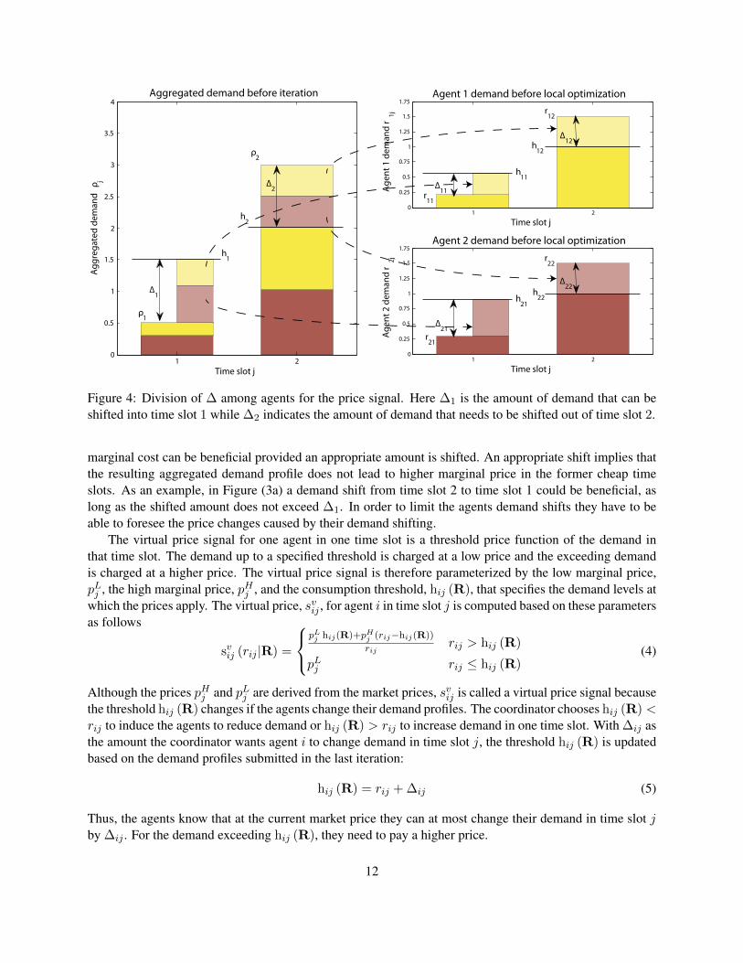
Figure 4: Division of ∆ among agents for the price signal. Here ∆1 is the amount of demand that can beshifted into time slot 1 while ∆2 indicates the amount of demand that needs to be shifted out of time slot 2.

marginal cost can be beneficial provided an appropriate amount is shifted. An appropriate shift implies thatthe resulting aggregated demand profile does not lead to higher marginal price in the former cheap timeslots. As an example, in Figure (3a) a demand shift from time slot 2 to time slot 1 could be beneficial, aslong as the shifted amount does not exceed ∆1. In order to limit the agents demand shifts they have to beable to foresee the price changes caused by their demand shifting.

The virtual price signal for one agent in one time slot is a threshold price function of the demand inthat time slot. The demand up to a specified threshold is charged at a low price and the exceeding demandis charged at a higher price. The virtual price signal is therefore parameterized by the low marginal price,pLj , the high marginal price, pHj , and the consumption threshold, hij (R), that specifies the demand levels atwhich the prices apply. The virtual price, svij , for agent i in time slot j is computed based on these parametersas follows

svij (rij |R) =

pLj hij(R)+pHj (rij−hij(R))

rijrij > hij (R)

pLj rij ≤ hij (R)(4)

Although the prices pHj and pLj are derived from the market prices, svij is called a virtual price signal becausethe threshold hij (R) changes if the agents change their demand profiles. The coordinator chooses hij (R) <rij to induce the agents to reduce demand or hij (R) > rij to increase demand in one time slot. With ∆ij asthe amount the coordinator wants agent i to change demand in time slot j, the threshold hij (R) is updatedbased on the demand profiles submitted in the last iteration:

hij (R) = rij + ∆ij (5)

Thus, the agents know that at the current market price they can at most change their demand in time slot jby ∆ij . For the demand exceeding hij (R), they need to pay a higher price.

12

1 20

0.5

1

1.5

2

2.5

3

3.5

4

Time slot j

Agg

rega

ted

dem

and

ρ j‚

Aggregated demand after iteration

1 20

0.25

0.5

0.75

1

1.25

1.5

1.75Agent 1 demand after local optimization

Time slot j

Age

nt 1

dem

and

r1j‚

h11

h12

r12‚

r11‚

1 20

0.25

0.5

0.75

1

1.25

1.5

1.75Agent 2 demand after local optimization

Time slot j

Age

nt 2

dem

and

r2j‚

h22h

21

r22‚

r21‚

h2

h1

ρ2‚

ρ1‚

Figure 5: Demand after agent’s local optimization. Agent 1 cannot reduce its entire demand from time slot2 (i.e., r12 > h12 because of its own consumption constraints (left top plot). Thus the aggregated load intime slot 1 is still below the threshold (i.e., ρ′1 < h1). Thus the central coordinator again sends a modifiedprice signal to the agents and the process continues until agents stop shifting their demands.

The demand, ∆j , the coordinator wants to change in time slot j is calculated as the difference betweenthe current aggregated demand and the threshold of the market price:

∆j = hj − ρj (6)

Since the coordinator wants the total load change of the agents to be less than ∆j the coordinator has toensure that

∑i ∆ij ≤ ∆j . The allowable shift for an agent is proportional to the agent’s share of the total

demand in that time slot, i.e., ∆ij =∆jrij∑

i rij. Figure 4 shows how the total load change is divided among the

agents in order to create the individual virtual price signals. The left side shows the initial aggregated loadsof two agents. The yellow load belongs to agent 1 and the red load to agent 2. Since the aggregated demandis below the threshold in time slot 1 (i.e., ρ1 < h1) and above the threshold in time slot 2 (i.e., ρ2 > h2),the coordinator wants the agents to shift demand from time slot 2 to time slot 1. The amount of demand thatcan be shifted into time slot 1 is ∆1 while ∆2 is the amount of demand that needs to be shifted out of timeslot 2. The right side shows the individual thresholds of the agents as determined by the central coordinatorusing the procedure described above. The allocation of the load change to the agents is illustrated by thedashed arrows. The current demand of agent 1 in time slot 1 is r11 and its threshold for time slot 1 is h11

(the other notations can be interpreted similarly).

4.1.3 The agent’s response to the virtual price signal

Having received the virtual price signal the firms will independently optimize their demand profiles in orderto minimize their cost according to Problem (3). Together with the virtual price signal the agents’ objective

13

function Cvi (ri|R) =

∑Mj=1 svij (rij |R) rij + gi(ri) can be written as:

Cvi (ri|R) =

M∑j=1

[pHj (rij − hij (R))+ + pLj (rij − hij (R))− + pLj hij (R)

]+ gi(ri) (7)

Since the virtual price signal divides the amounts to be shifted among the agents so that the agents have topay the high price pHj for demand exceeding their individual threshold, no agent will shift too much demand,based on a false impression of possible cost reduction. Figure 5 shows the agents’ demand profiles after theirindividual optimization. The left side shows the individual problems of the agents, after they have optimizedtheir demand profile according to their virtual price signal. In comparison to Figure 4 on the right side it canbe seen that agent 2 shifted the whole amount as was allocated, but agent 1 only shifted some part of it, dueto its constraints. The right side shows the central problem after the agents’ individual optimization. It canbe seen that there is still demand left to be shifted from time slot 2 to time slot 1. This remaining demandwould again be divided among the agents in the subsequent iteration.

4.2 Convergence of the basic algorithm

In this section we prove that the basic iterative procedure always converges to an optimal solution in thebasic setting with M = 2 and gi(·) = 0. In Lemma 1, it is shown that the algorithm strictly reduces costin every iteration. This fact will be used in Theorem 1 to show that the algorithm always converges. Thenin Theorem 2 it is shown that, when M = 2 and gi(·) = 0, the converged solution is an optimal solution.Subsequently it is shown that the algorithm can get stuck in a suboptimal solution in general settings ifM > 2 (Lemma 2) or if gi(·) 6= 0 (Lemma 3).

Lemma 1. The algorithm strictly reduces the total cost in every iteration: C (R′) < C (R).

Proof. Let’s first introduce some notation that will be used throughout this proof. Let R be the demandprofile at the end of iteration round t and R′ be the demand profile at the end of round t + 1. Similarly,let C(R) be the electricity cost at the end of iteration round t and C(R′) be the electricity cost at the endof round t + 1. The virtual prices for round t + 1 are computed by the central manager using R. LetCvi (ri|R) be the cost of electricity for agent i computed according to the virtual price signal for demands at

the beginning of round t+ 1 and Cvi (r′i|R) at the end of round t+ 1.

At the beginning of each iteration the total cost (given by the objective function in Problem (2)) for theconsumer group based on market prices is equal to the sum of the individual cost of the agents (give by the

14

objective function in Problem (3)) based on the virtual price signals∑N

i=1 Cvi (ri|R) = C (R):

N∑i=1

M∑j=1

svij (rij |R) rij +

N∑i=1

gi(ri)

=N∑i=1

M∑j=1

[pHj

(rij −

(rij +

(hj − ρj) rij∑i rij

))+

+ pLj

(rij −

(rij +

(hj − ρj) rij∑i rij

))−+ pLj

(rij +

(hj − ρj) rij∑i rij

)]+

N∑i=1

gi(ri)

=

M∑j=1

[pHj (ρj − hj)+ + pLj (ρj − hj)− + pLj hj

]+

N∑i=1

gi(ri)

=N∑i=1

M∑j=1

pj (ρj) rij +N∑i=1

gi(ri)

(8)

If the algorithm has not stopped, at least one agent has changed its demand profile, i.e., ∃i with r′i 6= ri.According to Problem (3) agents only change their demand profile, if that reduces their cost. Thus, giventhe virtual price signal for agent i the cost of the new demand profile r′i is strictly lower than of its previousdemand profile ri:

Cvi

(r′i|R

)< Cv

i (ri|R) (9)

After all agents have submitted their new demand profile the new aggregated demand is computed as: ρ′j =∑Ni=1 r

′ij . Next we show that the sum of the agents’ individual cost according to the virtual price signals

is an upper bound on the total central cost at market prices. Thus, the total cost given the new aggregateddemand is also lower or equal to the sum of the agents’ individual cost given their new demand. This fact isvery important, because it prevents the herding behavior: No solution that reduces the cost for the agents’individual problems can lead to a worse solution in the central problem. This is proved by showing withEquations (1) and (7) that for every time slot j the difference between the total cost for the aggregateddemand and the sum of the agents’ individual cost is less than or equal to 0. The following is a sketch of theproof omitting some algebraic steps for the ease of readability. Please consult Appendix A for the completeproof. For any time slot, j, we have

N∑i=1

pj

(ρ′j)r′ij −

N∑i=1

svij(r′ij |R

)r′ij

=

∑N

i: r′ij≤hij

(pHj − pLj

)(r′ij − hij (R)

)ρ′j > hj∑N

i: r′ij>hij

(pLj − pHj

)(r′ij − hij (R)

)ρ′j ≤ hj

=

[∑N

i=1

(pHj − pLj

)(r′ij − hij (R)

)−]≤ 0 ρ′j > hj[∑N

i=1

(pLj − pHj

)(r′ij − hij (R)

)+]≤ 0 ρ′j ≤ hj

(10)

15

Since∑N

i=1 pj

(ρ′j

)r′ij ≤

∑Ni=1 svij

(r′ij |R

)r′ij ∀j, it also holds for the sum of all time slots: C (R′) ≤∑N

i=1 Cvi (r′i|R). From Equations 8, 9 and 10 we can conclude that:

C(R′)≤

N∑i=1

Cvi

(r′i|R

)<

N∑i=1

Cvi (ri|R) = C (R) (11)

Thus, the total cost is strictly reduced in each iteration.

Theorem 1. The basic iterative algorithm for solving problem (2) always converges for any value of M .

Proof. From the definition we have that Problem (2) is convex and a lower bound on the total cost can beobtained by the sum of the individual initial demand profile costs at market prices. From Lemma 1 wehave that the algorithm reduces the total cost in each iteration. Thus, it can be concluded that the algorithmconverges.

Theorem 2. Assuming the basic setting with M = 2 and gi(·) = 0, the converged solution of the basicalgorithm R is optimal.

Proof. We now prove by contradiction that when the algorithm has converged to the solution R, then thereis no other solution, R′, with lower cost. Assume there exists a solution R′ with C(R′) < C(R). Let the 2time slots be {j, k}, where ρ′j < ρj and ρ′k > ρk (without loss of generality). Note that pm

j (ρj) > pmk (ρk),

because otherwise the new cost would not be lower. In the proof below, three cases are considered.First, if ρj 6= hj , ρk 6= hk we get that all agents have active constraints such that a shift from j to k

would be infeasible for the agents, because otherwise a shift from j to k would be beneficial for at leastone agent and the algorithm would not have stopped. Since there is no feasible shift from j to k it followsρ′j ≥ ρj and ρ′k ≤ ρk. With C(R′) < C(R) it follows that pm

j (ρj) < pmk (ρk), which leads to a contradiction

since our assumption implies that pmj (ρj) > pmk (ρk).If ρj = hj , ρk = hk then pm

j (ρj) = pLj (as ρj decreases) and pmk (ρk) = pHk (as ρk increases). From the

market price structure we have pHk > pLj . It follows pmj (ρj) < pm

k (ρk), which leads to a contradiction.If ρj 6= hj , ρk = hk and if ρj < hj then pm

j (ρj) = pLj and pmk (ρk) = pHk thus pm

j (ρj) < pmk (ρk).

If ρj > hj then pmj (ρj) = pHj and pm

k (ρk) = pHk . We have pHk > pHj , because otherwise a shift fromj to k would be beneficial for at least one agent and the algorithm would not have stopped. It followspmj (ρj) < pm

k (ρk), which again leads to a contradiction. The case of ρj = hj , ρk 6= hk works similarly.It follows that R is the optimal solution, as no solution with lower cost exists. Thus, the proposed

iterative algorithm converges to the optimal solution. Since the problem is convex that solution is also theglobal optimal solution (Boyd & Vandenberghe, 2004).

Lemma 2. The basic algorithm can converge to a suboptimal solution in settings with M > 2.

Proof. We now prove by presenting a counterexample that the basic algorithm can converge to a suboptimalsolution in general settings with M > 2. Consider a population of 2 agents, N = 2, and a planning horizonof 3 time slots,M = 3. The agents’ constraints are in a form so that in the converged solution the aggregateddemand is below the threshold in one time slot, directly at the threshold in another time slot and in one timeslot above the threshold. Let the price function for the three time slots be given as:

(pL1 , pH1 ) = (3, 6), h1 = 10

(pL2 , pH2 ) = (2, 5), h2 = 10

(pL3 , pH3 ) = (1, 4), h3 = 10

16

The individual constraints on the agents’ consumption are: (a) upper and lower bounds on the demand ineach time slot and (b) the total consumption over all time slots is constant. Specifically,

r11 ∈ [0, 3], r12 ∈ [0, 10], r13 ∈ [0, 10], r11 + r12 + r13 = τ1 = 17

r21 ∈ [0, 10], r22 ∈ [0, 10], r23 ∈ [9, 15], r21 + r22 + r23 = τ2 = 17

Let R(t) denote the demand profile of the agents in the tth iteration and let t = 1 be the initial iterationand t = T be the final iteration at convergence. At the beginning the agents compute their initial demandprofiles based on the market prices r(1)

1 = (0, 7, 10), r(1)2 = (0, 2, 15). The cost based on the initial demand

profiles is C(R(1)

)= 88.

At convergence the final profiles of the two agents are r(T )1 = (3, 7 + 7

9 , 6 + 29), r(T )

2 = (5 + 79 , 2 + 2

9 , 9)

(see Figure 6a for a graphical representation). The cost based on these demand profiles is C(R(T )

)= 77+2

9 .However a different demand profile of the agents exists with r′1 = (3, 10, 4), r′2 = (7, 0, 10) (see

Figure 6b for a graphical representation). This profile is feasible and leads to lower total cost C (R′) = 76.It follows that the algorithm has stopped in a suboptimal solution.

Lemma 3. The basic algorithm can converge to a suboptimal solution in settings with gi(·) 6= 0.

Proof. In Appendix B a counterexample is presented, to prove that the basic algorithm can converge to asuboptimal solution in general settings with gi(·) 6= 0.

5 General Coordination Algorithm

In the previous sections we introduced a basic iterative coordination algorithm for optimal energy allocationin the basic setting with a planning horizon of only two time slots, M = 2, and no cost for shifting demand,g(·) = 0. Moreover we presented counter examples which show that in general settings with M > 2 org(·) 6= 0 the algorithm can get stuck in a suboptimal solution. In this section we will present a generalcoordination algorithm, for the energy allocation in general settings with more than two time slots and non-zero individual costs, g(·) 6= 0, for shifting demand. First, using an example, we explain the reason forthe basic algorithm to get stuck at a sub-optimal solution in the general settings. Then we introduce anadditional phase to the basic algorithm and state the general algorithm. Subsequently in Theorem 3 weprove that the converged solution of the general algorithm is optimal in general settings.

5.1 The additional phase

The reason for convergence to a suboptimal solution is that the coordinator cannot determine the agents’marginal valuation for their demand, if the aggregated demand is at a threshold. The coordinator onlyknows that their marginal valuations are somewhere in between the low price below the threshold pLj andthe high price above the threshold pHj . However the agents might have different valuations so that a shiftfrom an agent with a lower valuation in that time slot to an agent with a higher valuation might be beneficial.The following examples illustrate the statements made above.

In the counterexample for proving Lemma 2 the aggregated demand in the final demand profile R(T )

is at the threshold in time slot 2. The demand profile in the converged profile is shown in Figure 6a. Thevaluation for one additional unit of energy in time slot 2 for the agents is given by the cost savings generatedby the possible reduction in the other time slots. The demand constraints of the agents for each time slotare indicated in Figure 6 by the dashed lines. In any time slot, the lower horizontal dashed line indicates

17

1 2 30

2

4

6

8

10

12

time slot

dem

and

agen

t 2

(KW

h)

1 2 30

2

4

6

8

10

12

time slot

dem

and

agen

t 1

(KW

h)

p1L=3 p2

L=2 p3L=1

p1H=6

p2H=5

p3H=4

(a) Converged Solution R(T )

1 2 30

2

4

6

8

10

12

time slotde

man

d ag

ent 2

(K

Wh)

1 2 30

2

4

6

8

10

12

time slot

dem

and

agen

t 1

(KW

h)

time slot

(b) Optimal Solution R′

Figure 6: Converged and Optimal solution for the example in Lemma 2. The top row shows the demand ofagent 1 and the bottom row the demand of agent 2. The dashed lines indicate the upper and lower bounds ofthe demands of the agents in a time slot.

the lower bound and the upper horizontal dashed line indicates the upper bound of the electricity demandof the agent. In order to increase demand in time slot 2 agent 1 could decrease demand in either time slot 1or 3. Since the marginal price for electricity is higher in time slot 3, agent 1’s valuation is 4. Because ofits constraints agent 2 can only decrease demand in time slot 1 so that its valuation is 3. Both valuationsare between the low price pL2 = 2 and the high price pH2 = 5, but agent 1’s valuation is higher thanagent 2’s. A shift from agent 2 to agent 1 would therefore reduce the total cost. However the coordinatordoes not know which agent has a higher valuation, because it does not know the agents’ constraints and thuscannot adjust the thresholds to induce the shift that would decrease the cost. The algorithm thus stops in asuboptimal solution. Similar reasoning can be used with the counterexample given for proving Lemma 3to understand why the basic algorithm may converge to a suboptimal solution when the individual costs forshifting demand is non-zero.

In order to resolve the problem arising when in the converged solution the aggregated demand is at athreshold in some time slots, let’s now introduce an additional phase to the algorithm. The basic idea of thisadditional phase is that the coordinator queries the agents for their individual valuation for an additional unitof energy in those time slots. The coordinator then uses this information to adjust the virtual price signals.

When the original algorithm has converged, the coordinator checks whether the aggregated demand is atthe threshold for at least one time slot. If that is not the case, the algorithm stops and the solution is optimal.However if the demand is at the threshold in some time slot, the coordinator initiates another iteration. Inthis iteration the coordinator sends an additional query to the agents besides the virtual price signal. Thecoordinator requests the agents’ marginal valuation for an increase and for a decrease of energy in all timeslots that are at the threshold.

18

Having received the virtual price signal and the additional request from the coordinator the agents com-pute their optimal demand profile r′i, based on the virtual price signal. In addition the agents compute thevectors v+

i and v−i . The vector v+i consists of a v+

ij(R) for every time slot at the threshold, ρj = hj ,indicating the change in cost that would occur to agent i if the coordinator would increase the threshold inthat time slot by ε. The vector v−i consists of a v−ij(R) for every time slot at the threshold indicating thechange in cost that would occur to agent i if the coordinator would decrease the threshold in that time slotby ε. After this computation the agents send ri, v+

i and v−i back to the coordinator.For the following analysis let Rij+ be the demand profile from which in the resulting individual cost

minimization problem of agent i the threshold in time slot j is increased by ε, hij(Rij+) = hij(R) + ε.Similarly let Rij− be the demand profile from which in the resulting individual cost minimization problemof agent i the threshold in j is decreased by ε, hij(Rij−) = hij(R) − ε. With that v+

ij(R) and v−ij(R) arecomputed as follows:

v+ij = Cv

i

(rj+i |R

ij+)− Ci(r

′i)

v−ij = Cvi

(rj−i |R

ij−)− Ci(r

′i)

(12)

Having received the demand profiles and marginal valuations of the agents the coordinator computesthe virtual price signals for the next iteration. If the aggregated demand is at the threshold, ρj = hj , the

coordinator finds the agent with the lowest cost for an ε raise of the threshold: l = arg mini

{v+ij

}and the

agent with the lowest cost for an ε reduction of the threshold: k = arg mini

{v−ij

}. If the combined change

in cost is negative v−kj + v+lj < 0, meaning a beneficial shift exists from agent l to agent k, the coordinator

updates the thresholds of agents l, k based on

∆lj = ε

∆kj = −ε

The algorithm stops when the demand is not at the threshold in any time slot or if for all time slots at thethresholds no such pair l, k exists with v−kj + v+

lj < 0. It follows that, when the algorithm converges, inevery time slot j with the aggregated demand at the threshold ρj = hj for all agents the cost reduction ofan increase of the threshold is less than the additional cost arising from a reduction of the threshold for allother agents

v+lj ≥ −v

−kj , ∀l, k ∈ {1, ..., N} and ∀j s.t. ρj = hj (13)

because otherwise the coordinator would change the price signals and the algorithm would not stop.

5.2 General algorithm

The general algorithm is designed as an iterative algorithm where the coordinator updates the virtual pricesignals based on the consumers’ feedback and thus gradually adjusts the individual demands to the centraloptimal solution. The overall algorithm is shown in Algorithm 1. Each iteration consists of two steps: First,the central coordinator aggregates the demand submitted by the agents and computes virtual price signalsfor each agent. The virtual price signals are computed in CalculateVirtualPriceSignals (Algorithm 2).Second, the individual agents use the virtual price signal to solve their individual cost optimization problemand compute their marginal valuation for their electricity demand and report them to the coordinator. Theagents’ response is computed in CalculateDemandProfileAndValuation (Algorithm 3).

19

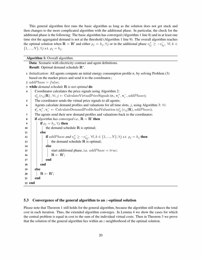
This general algorithm first runs the basic algorithm as long as the solution does not get stuck andthen changes to the more complicated algorithm with the additional phase. In particular, the check for theadditional phase is the following: The basic algorithm has converged (Algorithm 1 line 8) and in at least onetime slot the aggregated demand is not at the threshold (Algorithm 1 line 9). The overall algorithm reachesthe optimal solution when R = R′ and either ρj = hj ,∀j or in the additional phase v+

lj ≥ −v−kj , ∀l, k ∈

{1, ..., N},∀j s.t. ρj = hj .

Algorithm 1: Overall algorithm.Data: Scenario with electricity contract and agent definitions.Result: Optimal demand schedule R∗.

1 Initialization: All agents compute an initial energy consumption profile ri by solving Problem (3)based on the market prices and send it to the coordinator.;

2 addPhase = false;3 while demand schedule R is not optimal do4 Coordinator calculates the price signals using Algorithm 2:

svij (rij |R) ,∀i, j ← CalculateVirtualPriceSignals (ri,v+i ,v

−i , addPhase);

5 The coordinator sends the virtual price signals to all agents;6 Agents calculate demand profiles and valuations for all time slots, j, using Algorithm 3: ∀i:

r′i,v+i ,v

−i ← CalculateDemandProfileAndValuation (svij (rij |R), addPhase);

7 The agents send their new demand profiles and valuations back to the coordinator;8 if algorithm has converged i.e., R = R′ then9 if ρj = hj ,∀j then

10 the demand schedule R is optimal;11 else12 if addPhase and v+

lj ≥ −v−kj , ∀l, k ∈ {1, ..., N}, ∀j s.t. ρj = hj then

13 the demand schedule R is optimal;14 else15 start additional phase, i.e. addPhase = true;16 R← R′;17 end18 end19 else20 R← R′;21 end22 end

5.3 Convergence of the general algorithm to an ε-optimal solution

Please note that Theorem 1 still holds for the general algorithm, because the algorithm still reduces the totalcost in each iteration. Thus, the extended algorithm converges. In Lemma 4 we show the cases for whichthe central problem is equal in cost to the sum of the individual virtual costs. Then in Theorem 3 we provethat the solution of the general algorithm lies within an ε-neighborhood of the optimal solution.

20

Algorithm 2: Calculation of the virtual price signal by the coordinator.

1 CalculateVirtualPriceSignals (ri,v+i ,v

−i , addPhase);

Data: demand profiles and valuations of all agents, riv+i ,v

−i , ∀i.

Result: virtual price signals for all agents, svij (rij |R) ,∀i, j.

2 Compute the aggregated demand: ρj ←∑N

i=1 rij ;3 Compute demand to be shifted in each time slot: ∆j ← hj − ρj ;4 Divide that demand among all agents: ∆ij ← ∆jrij∑

i rij;

5 if addPhase then6 Find time slot j and agents l, k s.t. min

{v+lj − v

−kj

};

7 Adapt demand to be shifted for agent l: ∆lj ← ε;8 Adapt demand to be shifted for agent k: ∆kj ← −ε;9 end

10 Compute thresholds based on demands to be shifted: hij ← rij + ∆ij ;

Algorithm 3: Calculation of the individual demand profiles and marginal valuation of energy for agenti.1 CalculateDemandProfileAndValuation (svij (rij |R), addPhase);

Data: virtual price signal svij (rij |R), j = 1, . . . ,M .Result: new demand profile r′i and valuations v+

i ,v−i .

2 Compute new demand profile r′i according to virtual price signal: ri = arg minxi∈Xi Cvi (xi|R);

3 if addPhase then4 foreach time slot j at the threshold, rij = hij do5 Compute valuation of increased threshold: v+

ij ← Cvi

(rj+i |Rij+

)− Cv

i (r′i|R);

6 Compute valuation of decreased threshold: v−ij ← Cvi

(rj−i |Rij−

)− Cv

i (r′i|R);

7 end8 end

Lemma 4. Given a virtual price signal svij (·|R) and a consumption profile {x1j , x2j , ...xNj} in a time slotj, the real market cost,

∑Ni=1 pj

(ΣNi=1xij

)xij , equals the virtual cost

∑Ni=1 svij (xij |R)xij , if either ∀i,

xij ≥ hij (R) or ∀i, xij ≤ hij (R).

Proof. We will prove this by simple algebraic calculations. Assume that either ∀i, xij ≥ hij (R) or ∀i,xij ≤ hij (R). From Equation (10) we get that the difference between the market cost and the virtual cost,∑N

i=1 pj

(ΣNi=1xij

)xij −

∑Ni=1 svij (xij |R)xij , is given by either

N∑i: xij≤hij

(pHj − pLj

)(xij − hij (R)) , if

N∑i=1

xij > hj

N∑i: xij>hij

(pLj − pHj

)(xij − hij (R)) , if

N∑i=1

xij ≤ hj

21

If∑N

i=1 xij > hj then by our assumption ∀i, xij ≥ hij (R) so that the two cost are equal. If∑N

i=1 xij ≤ hjthen by our assumption ∀i, xij ≤ hij (R) so that the two cost are equal. It follows that the market costequals the virtual cost.

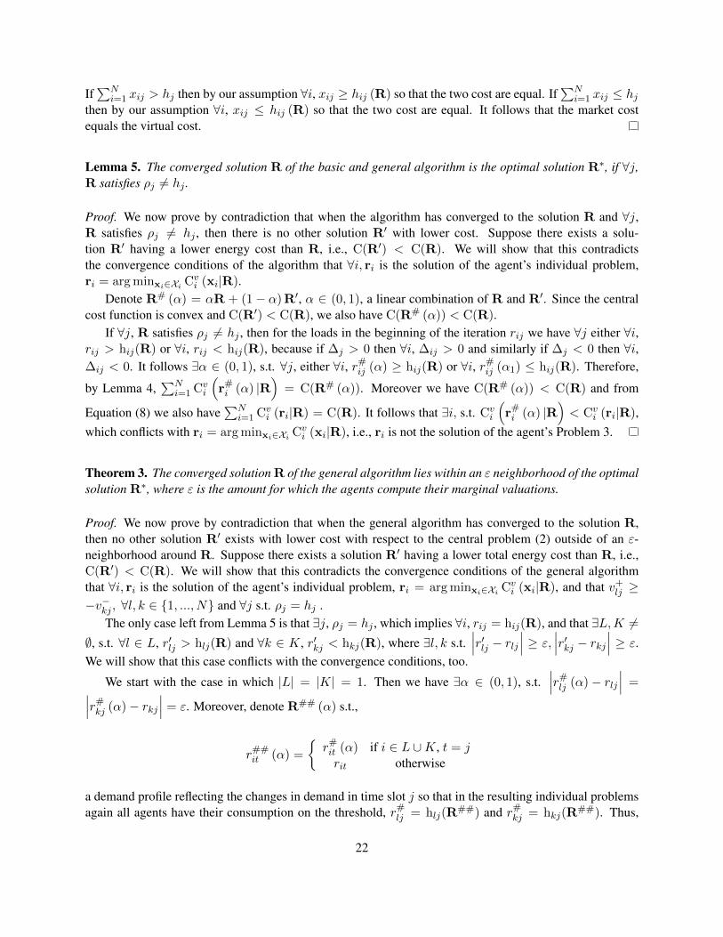
Lemma 5. The converged solution R of the basic and general algorithm is the optimal solution R∗, if ∀j,R satisfies ρj 6= hj .

Proof. We now prove by contradiction that when the algorithm has converged to the solution R and ∀j,R satisfies ρj 6= hj , then there is no other solution R′ with lower cost. Suppose there exists a solu-tion R′ having a lower energy cost than R, i.e., C(R′) < C(R). We will show that this contradictsthe convergence conditions of the algorithm that ∀i, ri is the solution of the agent’s individual problem,ri = arg minxi∈Xi Cv

i (xi|R).Denote R# (α) = αR + (1− α)R′, α ∈ (0, 1), a linear combination of R and R′. Since the central

cost function is convex and C(R′) < C(R), we also have C(R# (α)) < C(R).If ∀j, R satisfies ρj 6= hj , then for the loads in the beginning of the iteration rij we have ∀j either ∀i,

rij > hij(R) or ∀i, rij < hij(R), because if ∆j > 0 then ∀i, ∆ij > 0 and similarly if ∆j < 0 then ∀i,∆ij < 0. It follows ∃α ∈ (0, 1), s.t. ∀j, either ∀i, r#

ij (α) ≥ hij(R) or ∀i, r#ij (α1) ≤ hij(R). Therefore,

by Lemma 4,∑N

i=1 Cvi

(r#i (α) |R

)= C(R# (α)). Moreover we have C(R# (α)) < C(R) and from

Equation (8) we also have∑N

i=1 Cvi (ri|R) = C(R). It follows that ∃i, s.t. Cv

i

(r#i (α) |R

)< Cv

i (ri|R),which conflicts with ri = arg minxi∈Xi Cv

i (xi|R), i.e., ri is not the solution of the agent’s Problem 3.

Theorem 3. The converged solution R of the general algorithm lies within an ε neighborhood of the optimalsolution R∗, where ε is the amount for which the agents compute their marginal valuations.

Proof. We now prove by contradiction that when the general algorithm has converged to the solution R,then no other solution R′ exists with lower cost with respect to the central problem (2) outside of an ε-neighborhood around R. Suppose there exists a solution R′ having a lower total energy cost than R, i.e.,C(R′) < C(R). We will show that this contradicts the convergence conditions of the general algorithmthat ∀i, ri is the solution of the agent’s individual problem, ri = arg minxi∈Xi Cv

i (xi|R), and that v+lj ≥

−v−kj , ∀l, k ∈ {1, ..., N} and ∀j s.t. ρj = hj .The only case left from Lemma 5 is that ∃j, ρj = hj , which implies ∀i, rij = hij(R), and that ∃L,K 6=

∅, s.t. ∀l ∈ L, r′lj > hlj(R) and ∀k ∈ K, r′kj < hkj(R), where ∃l, k s.t.∣∣∣r′lj − rlj∣∣∣ ≥ ε,

∣∣∣r′kj − rkj∣∣∣ ≥ ε.We will show that this case conflicts with the convergence conditions, too.

We start with the case in which |L| = |K| = 1. Then we have ∃α ∈ (0, 1), s.t.∣∣∣r#

lj (α)− rlj∣∣∣ =∣∣∣r#

kj (α)− rkj∣∣∣ = ε. Moreover, denote R## (α) s.t.,

r##it (α) =

{r#it (α) if i ∈ L ∪K, t = jrit otherwise

a demand profile reflecting the changes in demand in time slot j so that in the resulting individual problemsagain all agents have their consumption on the threshold, r#

lj = hlj(R##) and r#

kj = hkj(R##). Thus,

22

with Lemma 4 we get that the sum of the virtual cost is equal to the central cost.

N∑i=1,i 6=l,k

Cvi

(r#i (α) |R

)+ Cv

l

(r#l (α) |R## (α)

)+ Cv

k

(r#k (α) |R## (α)

)= C(R# (α))

< C(R) =

N∑i=1

Cvi (ri|R)

which implies either

N∑i=1,i 6=l,k

Cvi

(r#i (α) |R

)<

N∑i=1,i 6=l,k

Cvi (ri|R)

⇒ ∃i, s.t.Cvi

(r#i (α) |R

)< Cv

i (ri|R)

which conflicts with the convergence condition ri = arg minxi∈Xi Cvi (xi|R);

or

Cvl

(r#l (α) |R## (α)

)+ Cv

k

(r#k (α) |R## (α)

)< Cv

l (rl|R) + Cvk (rk|R)

⇒ Cvl

(r#l (α) |R## (α)

)− Cv

l (rl|R) < −[Cvk

(r#k (α) |R## (α)

)− Cv

k (rk|R)]

For∣∣∣r#

kj (α)− rkj∣∣∣ = εwe get that Cv

l

(r#l (α) |R## (α)

)is equal to Cv

l

(rj+l |R

ij+)

and Cvk

(r#k (α) |R## (α)

)is equal to Cv

k

(rj−k |R

ij−)

. Thus, with Equation (12) follows

v+lj (R) < −v−kj (R)

which conflicts with the convergence condition, ∀l, k ∈ {1, 2, · · · , N}, v+lj (R) ≥ −v−kj (R).

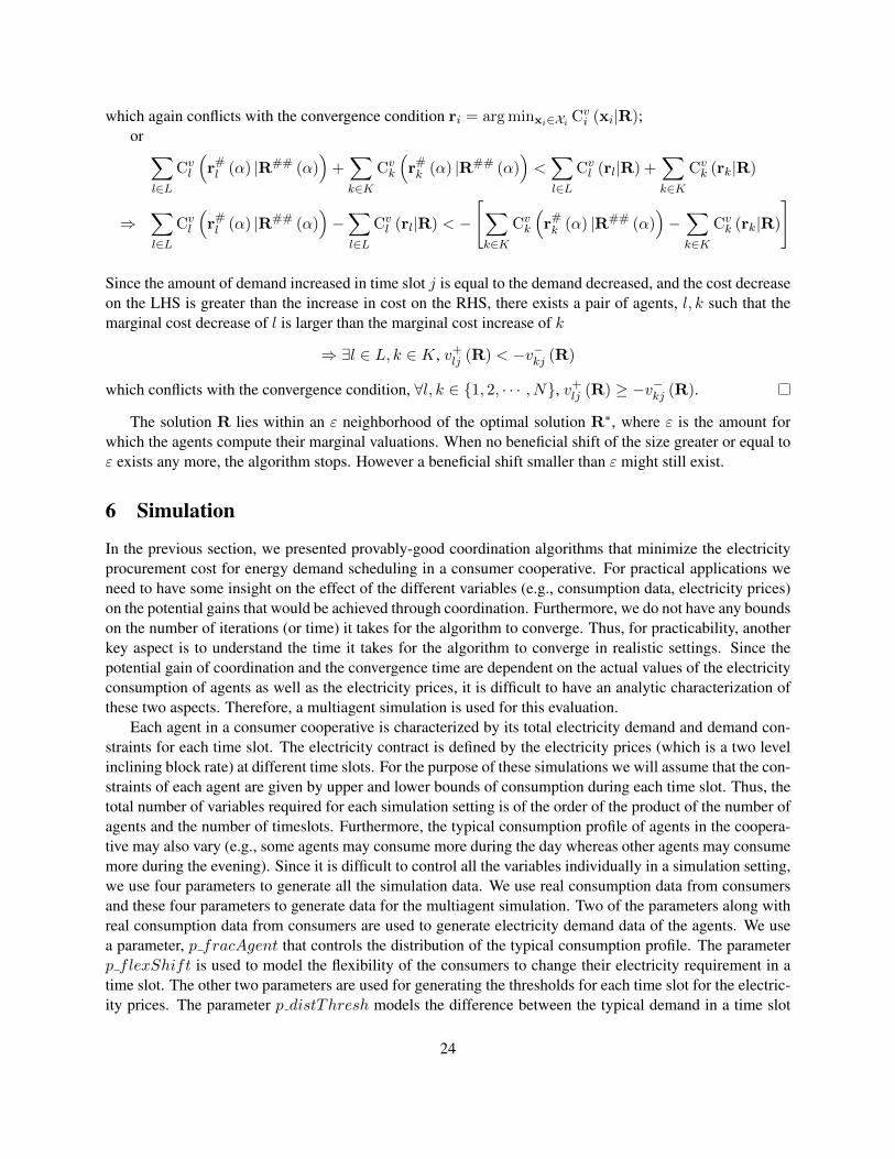
For the general case of |L| , |K| ≥ 1, we can get

N∑i=1,i/∈L∪K

Cvi

(r#i (α) |R

)+∑l∈L

Cvl

(r#l (α) |R## (α)

)+∑k∈K

Cvk

(r#k (α) |R## (α)

)= C(R# (α))

< C(R) =

N∑i=1

Cvi (ri|R)

which implies either

N∑i=1,i/∈L∪K

Cvi

(r#i (α) |R

)<

N∑i=1,i/∈L∪K

Cvi (ri|R)

⇒ ∃i, s.t.Cvi

(r#i (α) |R

)< Cv

i (ri|R)

23

which again conflicts with the convergence condition ri = arg minxi∈Xi Cvi (xi|R);

or ∑l∈L

Cvl

(r#l (α) |R## (α)

)+∑k∈K

Cvk

(r#k (α) |R## (α)

)<∑l∈L

Cvl (rl|R) +

∑k∈K

Cvk (rk|R)

⇒∑l∈L

Cvl

(r#l (α) |R## (α)

)−∑l∈L

Cvl (rl|R) < −

[∑k∈K

Cvk

(r#k (α) |R## (α)

)−∑k∈K

Cvk (rk|R)

]

Since the amount of demand increased in time slot j is equal to the demand decreased, and the cost decreaseon the LHS is greater than the increase in cost on the RHS, there exists a pair of agents, l, k such that themarginal cost decrease of l is larger than the marginal cost increase of k

⇒ ∃l ∈ L, k ∈ K, v+lj (R) < −v−kj (R)

which conflicts with the convergence condition, ∀l, k ∈ {1, 2, · · · , N}, v+lj (R) ≥ −v−kj (R).

The solution R lies within an ε neighborhood of the optimal solution R∗, where ε is the amount forwhich the agents compute their marginal valuations. When no beneficial shift of the size greater or equal toε exists any more, the algorithm stops. However a beneficial shift smaller than ε might still exist.

6 Simulation

In the previous section, we presented provably-good coordination algorithms that minimize the electricityprocurement cost for energy demand scheduling in a consumer cooperative. For practical applications weneed to have some insight on the effect of the different variables (e.g., consumption data, electricity prices)on the potential gains that would be achieved through coordination. Furthermore, we do not have any boundson the number of iterations (or time) it takes for the algorithm to converge. Thus, for practicability, anotherkey aspect is to understand the time it takes for the algorithm to converge in realistic settings. Since thepotential gain of coordination and the convergence time are dependent on the actual values of the electricityconsumption of agents as well as the electricity prices, it is difficult to have an analytic characterization ofthese two aspects. Therefore, a multiagent simulation is used for this evaluation.

Each agent in a consumer cooperative is characterized by its total electricity demand and demand con-straints for each time slot. The electricity contract is defined by the electricity prices (which is a two levelinclining block rate) at different time slots. For the purpose of these simulations we will assume that the con-straints of each agent are given by upper and lower bounds of consumption during each time slot. Thus, thetotal number of variables required for each simulation setting is of the order of the product of the number ofagents and the number of timeslots. Furthermore, the typical consumption profile of agents in the coopera-tive may also vary (e.g., some agents may consume more during the day whereas other agents may consumemore during the evening). Since it is difficult to control all the variables individually in a simulation setting,we use four parameters to generate all the simulation data. We use real consumption data from consumersand these four parameters to generate data for the multiagent simulation. Two of the parameters along withreal consumption data from consumers are used to generate electricity demand data of the agents. We usea parameter, p fracAgent that controls the distribution of the typical consumption profile. The parameterp flexShift is used to model the flexibility of the consumers to change their electricity requirement in atime slot. The other two parameters are used for generating the thresholds for each time slot for the electric-ity prices. The parameter p distThresh models the difference between the typical demand in a time slot

24

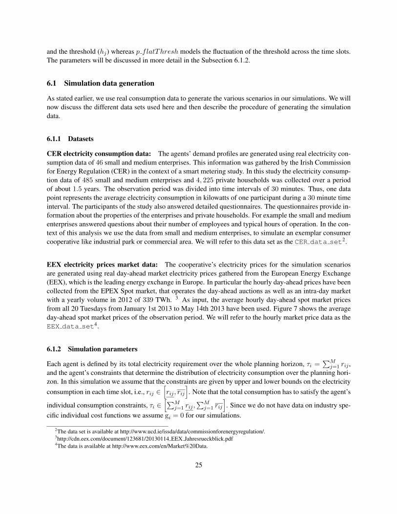
and the threshold (hj) whereas p flatThresh models the fluctuation of the threshold across the time slots.The parameters will be discussed in more detail in the Subsection 6.1.2.

6.1 Simulation data generation

As stated earlier, we use real consumption data to generate the various scenarios in our simulations. We willnow discuss the different data sets used here and then describe the procedure of generating the simulationdata.

6.1.1 Datasets

CER electricity consumption data: The agents’ demand profiles are generated using real electricity con-sumption data of 46 small and medium enterprises. This information was gathered by the Irish Commissionfor Energy Regulation (CER) in the context of a smart metering study. In this study the electricity consump-tion data of 485 small and medium enterprises and 4, 225 private households was collected over a periodof about 1.5 years. The observation period was divided into time intervals of 30 minutes. Thus, one datapoint represents the average electricity consumption in kilowatts of one participant during a 30 minute timeinterval. The participants of the study also answered detailed questionnaires. The questionnaires provide in-formation about the properties of the enterprises and private households. For example the small and mediumenterprises answered questions about their number of employees and typical hours of operation. In the con-text of this analysis we use the data from small and medium enterprises, to simulate an exemplar consumercooperative like industrial park or commercial area. We will refer to this data set as the CER data set2.

EEX electricity prices market data: The cooperative’s electricity prices for the simulation scenariosare generated using real day-ahead market electricity prices gathered from the European Energy Exchange(EEX), which is the leading energy exchange in Europe. In particular the hourly day-ahead prices have beencollected from the EPEX Spot market, that operates the day-ahead auctions as well as an intra-day marketwith a yearly volume in 2012 of 339 TWh. 3 As input, the average hourly day-ahead spot market pricesfrom all 20 Tuesdays from January 1st 2013 to May 14th 2013 have been used. Figure 7 shows the averageday-ahead spot market prices of the observation period. We will refer to the hourly market price data as theEEX data set4.

6.1.2 Simulation parameters

Each agent is defined by its total electricity requirement over the whole planning horizon, τi =∑M

j=1 rij ,and the agent’s constraints that determine the distribution of electricity consumption over the planning hori-zon. In this simulation we assume that the constraints are given by upper and lower bounds on the electricityconsumption in each time slot, i.e., rij ∈

[rij , rij

]. Note that the total consumption has to satisfy the agent’s

individual consumption constraints, τi ∈[∑M

j=1 rij ,∑M

j=1 rij

]. Since we do not have data on industry spe-

cific individual cost functions we assume gi = 0 for our simulations.

2The data set is available at http://www.ucd.ie/issda/data/commissionforenergyregulation/.3http://cdn.eex.com/document/123681/20130114 EEX Jahresrueckblick.pdf4The data is available at http://www.eex.com/en/Market%20Data.

25

1 2 3 4 5 6 7 8 9 10 11 12 13 14 15 16 17 18 19 20 21 22 23 242

2.5

3

3.5

4

4.5

5

5.5

6

6.5

7

time (hour of the day)

pric

e

(Eur

o ce

nts/

kWh)

day−ahead spot market price

Figure 7: Day-ahead spot market prices from EPEX Spot for an average Tuesday in 2013

Modeling the diversity of cooperatives: There are a variety of possible individual demand characteristicsof agents in a cooperative. However the consumption patterns of some customers may be more similar thanothers. To reflect this diversity of the agents within the simulations, we used the CER data set to identifytwo important classes of consumers with shared characteristics. Here, Class 1 represents consumers thatconsume most of their electricity during the day and have a low load at night, whereas Class 2 representsconsumers that have a stable consumption during the day, but have a higher consumption at night. With theseclasses different scenarios with varying compositions for the consumer cooperatives can be simulated. Thefraction of agent in Class 1 is defined by p fracAgent ∈ (0, 1). Thus, the fraction of agents from Class 2 is1−p fracAgent. The parameter p fracAgent allows us to vary the composition of the cooperative acrossthe different simulations.

To find the classes of consumers with similar characteristics the participants of the CER study wereclustered using a semi-automatic approach. In a first step the participants were clustered using k-meansclustering based on the information from the questionnaires and the electricity consumption data. From thequestionnaires the area of business, number of employees, approximate hours of operation and whether thepremises also operate during the weekends were taken into account for the clustering. From the electricityconsumption data the consumption profiles of Tuesdays were used, since the planning horizon in the scopeof this paper is one day and Tuesday is the most average work day with no effects like businesses whichdo not operate on Mondays. Note that the intention of the clustering was not to find a model that fits allparticipants into classes, but only to identify important classes of consumers to populate the simulations.Thus, in a second step the two classes were separated manually. The separation was based on the clusteringresults showing that a group of participants exists with a significant consumption profile during the day andanother group exists with participants mainly consuming during the night (see Figure 8).

Modeling the flexibility of consumers: Given the class of an agent, we generate the demand profile ofthe agent based on the real consumption data. Although the consumption data in the CER data set is

26

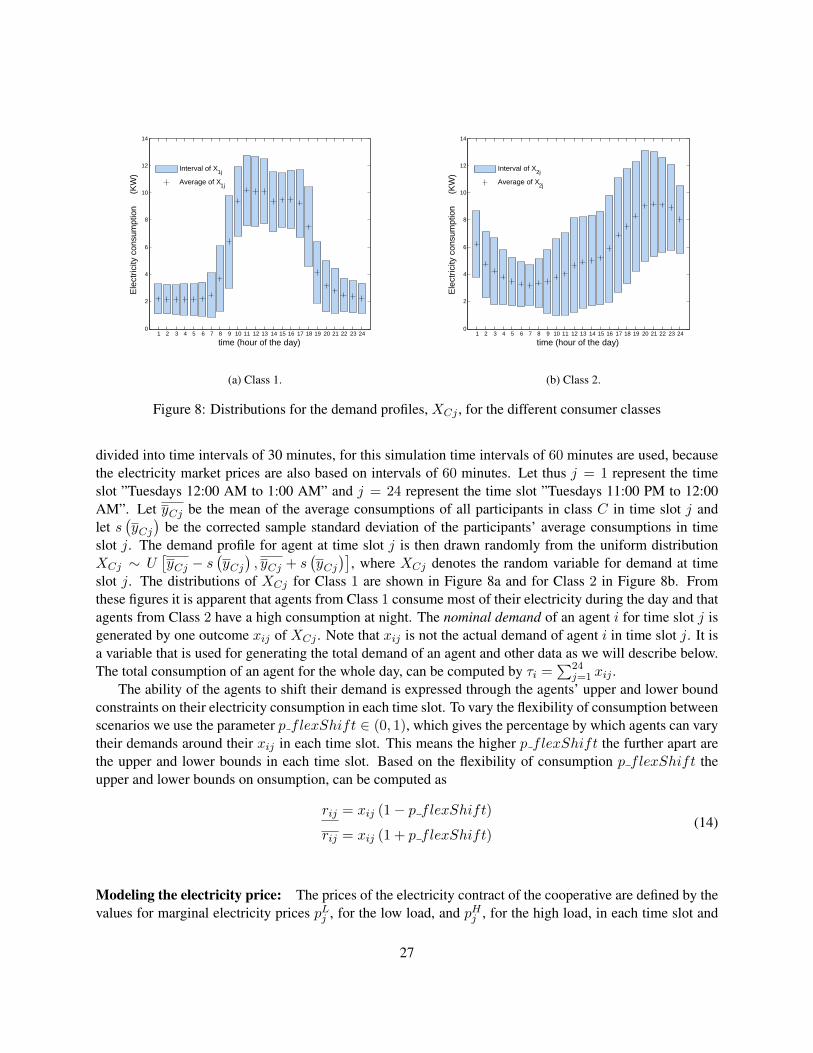
1 2 3 4 5 6 7 8 9 10 11 12 13 14 15 16 17 18 19 20 21 22 23 240

2

4

6

8

10

12

14

time (hour of the day)

Ele

ctric

ity c

onsu

mpt

ion

(

KW

)

Interval of X1j

Average of X1j

(a) Class 1.

1 2 3 4 5 6 7 8 9 10 11 12 13 14 15 16 17 18 19 20 21 22 23 240

2

4

6

8

10

12

14

time (hour of the day)

Ele

ctric

ity c

onsu

mpt

ion

(

KW

)

Interval of X2j

Average of X2j

(b) Class 2.

Figure 8: Distributions for the demand profiles, XCj , for the different consumer classes

divided into time intervals of 30 minutes, for this simulation time intervals of 60 minutes are used, becausethe electricity market prices are also based on intervals of 60 minutes. Let thus j = 1 represent the timeslot ”Tuesdays 12:00 AM to 1:00 AM” and j = 24 represent the time slot ”Tuesdays 11:00 PM to 12:00AM”. Let yCj be the mean of the average consumptions of all participants in class C in time slot j andlet s

(yCj

)be the corrected sample standard deviation of the participants’ average consumptions in time

slot j. The demand profile for agent at time slot j is then drawn randomly from the uniform distributionXCj ∼ U

[yCj − s

(yCj

), yCj + s

(yCj

)], where XCj denotes the random variable for demand at time

slot j. The distributions of XCj for Class 1 are shown in Figure 8a and for Class 2 in Figure 8b. Fromthese figures it is apparent that agents from Class 1 consume most of their electricity during the day and thatagents from Class 2 have a high consumption at night. The nominal demand of an agent i for time slot j isgenerated by one outcome xij of XCj . Note that xij is not the actual demand of agent i in time slot j. It isa variable that is used for generating the total demand of an agent and other data as we will describe below.The total consumption of an agent for the whole day, can be computed by τi =

∑24j=1 xij .

The ability of the agents to shift their demand is expressed through the agents’ upper and lower boundconstraints on their electricity consumption in each time slot. To vary the flexibility of consumption betweenscenarios we use the parameter p flexShift ∈ (0, 1), which gives the percentage by which agents can varytheir demands around their xij in each time slot. This means the higher p flexShift the further apart arethe upper and lower bounds in each time slot. Based on the flexibility of consumption p flexShift theupper and lower bounds on onsumption, can be computed as

rij = xij (1− p flexShift)

rij = xij (1 + p flexShift)(14)

Modeling the electricity price: The prices of the electricity contract of the cooperative are defined by thevalues for marginal electricity prices pLj , for the low load, and pHj , for the high load, in each time slot and

27

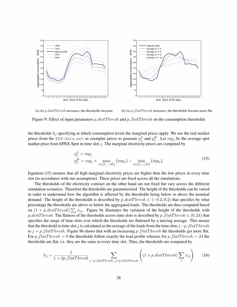
1 2 3 4 5 6 7 8 9 10 11 12 13 14 15 16 17 18 19 20 21 22 23 240

50

100

150

200

250

300

350

400

450

500

time (hour of the day)

aggr

eaga

ted

cons

umpt

ion

(K

W)

−20%−10%original profile+10%+20%

(a) As p distThresh increases, the thresholds increase.

1 2 3 4 5 6 7 8 9 10 11 12 13 14 15 16 17 18 19 20 21 22 23 240

50

100

150

200

250

300

350

400

450

500

time (hour of the day)

aggr

eaga

ted

cons

umpt

ion

(K

W)

original profileaverage of +/−3average of +/−6average of +/−9average of +/−12

(b) As p flatThresh increases, the thresholds become more flat.

Figure 9: Effect of input parameters p distThresh and p flatThresh on the consumption thresholds

the thresholds hj specifying at which consumption levels the marginal prices apply. We use the real marketprices from the EEX data set as exemplar prices to generate pLj and pHj . Let mpj be the average spotmarket price from EPEX Spot in time slot j. The marginal electricity prices are computed by

pLj = mpj

pHj = mpj + maxx∈{1,...,M}

{mpx} − minx∈{1,...,M}

{mpx}(15)

Equation (15) ensures that all high marginal electricity prices are higher than the low prices in every timeslot (in accordance with our assumption). These prices are fixed across all the simulations.

The thresholds of the electricity contract on the other hand are not fixed but vary across the differentsimulation scenarios. Therefore the thresholds are parameterized. The height of the thresholds can be variedin order to understand how the algorithm is affected by the thresholds being below or above the nominaldemand. The height of the thresholds is described by p distThresh ∈ (−0.2, 0.2) that specifies by whatpercentage the thresholds are above or below the aggregated loads. The thresholds are thus computed basedon (1 + p distThresh)

∑i xij . Figure 9a illustrates the variation of the height of the thresholds with

p distThresh. The flatness of the thresholds across time slots is described by p flatThresh ∈ (0, 24) thatspecifies the range of time slots over which the thresholds are flattened by a moving average. This meansthat the threshold in time slot j is calculated as the average of the loads from the time slots j−p flatThreshto j + p flatThresh. Figure 9b shows that with an increasing p flatThresh the thresholds get more flat.For p flatThresh = 0 the thresholds follow exactly the load profile whereas for p flatThresh = 24 thethresholds are flat, i.e. they are the same in every time slot. Thus, the thresholds are computed by

hj =1

1 + 2p flatThresh

∑j−p flatThresh, j+p flatThresh

((1 + p distThresh)

∑i

xij

)(16)

28

Simulation scenarios: To create different consumer cooperative scenarios, the input parameters were var-ied as follows: p fracAgent ∈ {0, 0.25, 0.5, 0.75, 1}, p flexShift ∈ {0.1, 0.2, 0.3}, p distThresh ∈{−0.2,−0.1, 0, 0.1, 0.2} and p flatThresh ∈ {0, 12, 24}. This resulted in a total of 225 different sce-narios. To reduce the variance in the results the simulations were repeated 4 times with different randomseeds. Our observations are based on the mean over the 4 repetitions. Additionally, in order to analyzethe convergence rate, the parameter ε was varied as ε ∈ {0.5, 1, 2} and the population size was varied as#agents ∈ {20, 40, 60, 80, 100}. The simulations were stopped at convergence of the algorithm, which forthis simulations was defined to be reached, when the cost reduction in one iteration got less than 0.00001%,C (R) /C (R′) < 1.0000001.

6.2 Simulation results

We will first present the effects of the different simulation parameters on the potential gain through coordi-nation and subsequently discuss the results on convergence time. The main purpose of this analysis of thepotential gains of coordination is that a coordinator of a real consumer cooperative can decide whether theimplementation of the coordination algorithm is beneficial for its cooperative. In addition, an indication ofthe potential gain can also help to decide on the composition of the cooperative.

For the evaluation we sampled a total of 225 scenarios. A subset of the results for p fracAgent =0, 0.5, 1 are shown in Figure 10. The x-axis represents the flexibility of shifting demand, the y-axis the flat-ness of the thresholds and the z-axis the height of the thresholds. In Figure 10a the results from cooperativesconsisting of consumers mainly consuming electricity at night are shown. In Figure 10b the results from thecooperatives that consist of both consumer classes in equal proportions are shown. Finally in Figure 10c theresults from the cooperatives consisting of only consumers with their main consumption during the day areshown. In all the figures there are scenarios with high cost reduction (white) and scenarios with less costreduction (dark red). Over all 225 scenarios a mean cost reduction of 2.62% was observed, with the resultsvarying from 0% to 7.06% cost reduction. The figures also allow a first guess on the effect of the differentparameters. First it can be seen that as the flexibility of shifting demand increases, i.e. p flexShift↗, thecost reduction increases. Second it can be seen that as the absolute distance from the thresholds to the loadprofile decreases, i.e. |p distThresh| ↘, cost reduction increases. From the composition of the coopera-tive, i.e. p fracAgent, as well as from the flatness of the thresholds, i.e. p flatThresh, no linear effectcan be observed. However there seems to be an effect of p fracAgent and p flatThresh together. Thisabsence of linear effect but presence of interaction effect is plausible, because when the thresholds followthe demand curve, the main difference of demand profiles between the agent populations get neutralized. Inorder to analyze these effects in detail a sensitivity analysis is performed.

6.2.1 Sensitivity analysis

The purpose of this sensitivity analysis is to understand the effect of the different input parameters on thepotential gain of coordination with the aim of developing trends that allow understanding the behavior ofthe system in scenarios that are not simulated. For the sensitivity analysis a multiple linear regression wasperformed to check the main effects of the input parameters and the cost reduction through coordination.The cost reduction as fraction of the initial cost was the dependent variable (criterion), the input param-eters p fracAgent, p flatThresh, p flexShift, the absolute value of the parameter p distThresh, i.e.|p distThresh|, and the interaction terms p distThresh∗p flexShift and p fracAgent∗p flatThreshwere included as independent variables (predictors) in the calculation. The input parameter p distThreshwas included as absolute values, because looking at the absolute distance is similar to separately looking at

29

0.10.2

0.3 012

24

−0.2

−0.1

0

0.1

0.2

p_flatThreshp_flexShift

p_di

stT

hres

h

0

0.01

0.02

0.03

0.04

0.05

0.06

0.07

(a) Only consumers who mainly consume at night,p fracAgent = 0.

0.10.2

0.3 012

24

−0.2

−0.1

0

0.1

0.2

p_flatThreshp_flexShift

p_di

stT

hres

h

0

0.01

0.02

0.03

0.04

0.05

0.06

0.07

(b) Consumers from both classes have equal fractions,p fracAgent = 0.5

0.10.2

0.3 012

24

−0.2

−0.1

0

0.1

0.2

p_flatThreshp_flexShift

p_di

stT

hres

h

0

0.01

0.02

0.03

0.04

0.05

0.06

0.07

(c) Only consumers who mainly consume during day,p fracAgent = 1.

Figure 10: The cost reduction through the coordination algorithm as a function of the four input parametersp fracAgent, p flatThresh, p distThresh and p flexShift

30

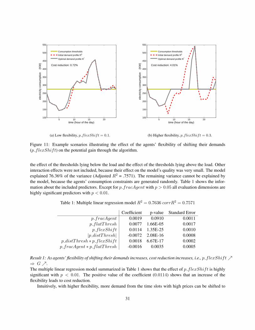
5 10 15 20100

150

200

250

300

350

400

450

500

550

time (hour of the day)

elec

tric

ity c

onsu

mpt

ion

(K

W)

Consumption thresholds

Initial demand profile R1

Optimal demand profile R*

Cost reduction: 0.72%

(a) Low flexibility, p flexShift = 0.1.

5 10 15 20100

150

200

250

300

350

400

450

500

550

time (hour of the day)

elec

tric

ity c

onsu

mpt

ion

(K

W)

Consumption thresholds

Initial demand profile R1

Optimal demand profile R*

Cost reduction: 4.01%

(b) Higher flexibility, p flexShift = 0.3.

Figure 11: Example scenarios illustrating the effect of the agents’ flexibility of shifting their demands(p flexShift) on the potential gain through the algorithm.

the effect of the thresholds lying below the load and the effect of the thresholds lying above the load. Otherinteraction effects were not included, because their effect on the model’s quality was very small. The modelexplained 76.36% of the variance (Adjusted R2 = .7571). The remaining variance cannot be explained bythe model, because the agents’ consumption constraints are generated randomly. Table 1 shows the infor-mation about the included predictors. Except for p fracAgent with p > 0.05 all evaluation dimensions arehighly significant predictors with p < 0.01.

Table 1: Multiple linear regression model R2 = 0.7636 corrR2 = 0.7571

Coefficient p-value Standard Errorp fracAgent 0.0019 0.0910 0.0011p flatThresh 0.0077 1.66E-05 0.0017p flexShift 0.0114 1.35E-25 0.0010

|p distThresh| -0.0072 2.08E-16 0.0008p distThresh ∗ p flexShift 0.0018 6.67E-17 0.0002p fracAgent ∗ p flatThresh -0.0016 0.0035 0.0005

Result 1: As agents’ flexibility of shifting their demands increases, cost reduction increases, i.e., p flexShift↗⇒ G↗.The multiple linear regression model summarized in Table 1 shows that the effect of p flexShift is highlysignificant with p < 0.01. The positive value of the coefficient (0.0114) shows that an increase of theflexibility leads to cost reduction.

Intuitively, with higher flexibility, more demand from the time slots with high prices can be shifted to

31

those time slots with lower prices and consequently a higher cost reduction can be achieved. For exampleif the flexibility is p flexShift = 0, no demand can be shifted and thus it is impossible to reduce thecost. While higher flexibility allows for more possibilities to coordinate the demand, there is another reasonfor the cost reduction. Recall that the gain of coordination is the difference between the cost resultingfrom the uncoordinated demand profile of the cooperative R1 and the coordinated demand profile R∗. Forcomputing R1 the agents optimize their demand according to the hourly market prices. Consequently, themore the agents’ flexibility of shifting demand increases the more the agents adapt their demand schedulesto the hourly prices. However, since the agents are not coordinated every agent shifts as much demand aspossible to cheap time slots. These demand shifts lead to load synchronization, where the total consumptionin the cheap slots exceeds the thresholds leading to higher consumption costs (herding behavior). Thus, highflexibility leads not only to more possibilities to coordinate the demand, but also to an uncoordinated profilewith highly synchronized demand. Figure 11 illustrates this effect in settings with low (p flexShift = 0.1)and higher (p flexShift = 0.3) flexibility. The figure shows clearly that the consumption peak is higherin the scenario with more flexibility. The area between the red dashed curve of the initial demand profileR1 and the optimal demand profile R∗ in gray multiplied by the respective marginal prices shows the costreduction through coordination. With the increasing freedom in Figure 11b it can be seen that the areabetween the two curves increases. Note that in the optimal demand profile the height of the peak is still thesame. The reason for this is that in the time slots below the thresholds the demand is at the upper bounds ofthe agents. Thus, there is a need for consumption above the thresholds. According to the hourly prices asdepicted in Figure 7 the cheapest remaining time slot is 17. Since the freedom allows demanding most ofthe remaining electricity in that time slot the height of the peak does not change.

Result 2: As the absolute distance of the consumption thresholds to the aggregated load profile decreases,cost reduction increases, i.e., |p distThresh| ↘ ⇒ G↗.The multiple linear regression model summarized in Table 1 shows that the effect of |p distThresh| ishighly significant with p < 0.01. The negative value of the coefficient (−0.0072) shows that the furtheraway the thresholds are to the load profile of the cooperative the less cost reduction can be achieved throughcoordination.

The group of consumers reduces its cost when they shift demand from time slots with the aggregateddemand above the threshold to time slots with the aggregated demand below the threshold. The maximumdemand that can possibly be shifted from the high consumption levels to the low consumption levels isgiven by the minimum of the demand above the thresholds and the unused demand below the thresholds.Intuitively, with the thresholds being above the load profile, the demand that can be shifted gets smaller,because the demand above the thresholds is smaller than the unused demand below the thresholds. Forexample in the extreme case where the thresholds are above the aggregated demand in every time slot, nobeneficial shift exists. Similarly, with the thresholds being below the load profile fewer possibilities to shiftexist, because the unused demand below the thresholds is smaller than the demand above the thresholds.Again, if the thresholds are below the aggregated demand in every time slot, no beneficial shift is possible.Consequently, the further away the thresholds are from the load profile the lower is the cost reduction thatcan be achieved. Figure 12 illustrates this effect in settings with low (p distThresh = −0.2), normal(p distThresh = 0) and high (p distThresh = 0.2) thresholds. The demand above the thresholds isrepresented by the area between the initial demand profile (red dashed line) and the thresholds (yellow flatline) above the thresholds, and the unused demand below the thresholds by the area between the two linesbelow the thresholds. This result is also effected by the flatness of the thresholds, i.e. p flatThresh,because the flatter the thresholds get, the larger the two described areas become. This would mean that withflatter thresholds the cost reduction increases as well. The multiple linear regression model summarized in

32

5 10 15 20100

150

200

250

300

350

400

450

500

550

time (hour of the day)

elec

tric

ity c

onsu

mpt

ion

(K

W)

Consumption thresholds

Initial demand pro�le R 1

Optimal demand pro�le R *

Cost reduction: 1.28%

(a) Thresholds below the load,p distThresh = −0.2.

5 10 15 20100

150

200

250

300

350

400

450

500

550

time (hour of the day)el

ectr

icity

con

sum

ptio

n

(KW

)

Consumption thresholds

Initial demand pro�le R 1

Optimal demand pro�le R *

Cost reduction: 4.01%

(b) Thresholds at load, p distThresh = 0.

5 10 15 20100

150

200

250

300

350

400

450

500

550

time (hour of the day)

elec

tric

ity c

onsu

mpt

ion

(K

W)

Consumption thresholds

Initial demand pro�le R 1

Optimal demand pro�le R *

Cost reduction: 5.83%

(c) Thresholds above the load,p distThresh = 0.2.

Figure 12: Example scenarios illustrating the effect of the distance of the thresholds to the load profiles(p distThresh) on the algorithm’s performance.

Table 1 supports this result, because it shows that the effect of p flatThresh is has a positive coefficient(0.0077) and is highly significant with p < 0.01.

However, the cost reduction in the scenario with high thresholds (p distThresh = 0.2) in Figure 12cis greater than in the case of thresholds with normal height (p distThresh = 0) in Figure 12b. Thisindicates that in addition to the decreased cost reduction caused by the absolute distance from the demandprofile there seems to be an effect that increases the cost reduction towards higher thresholds. In order tounderstand the positive effect towards higher thresholds, the flexibility of shifting demand has to be takeninto account. The regression model summarized in Table 1 shows that the effect of the interaction termp distThresh ∗ p flexShift is highly significant with p < 0.01. When the flexibility is low, it mighthappen that not the whole intended demand can be shifted. That is because the agents hit their lowerconsumption bounds in the time slots above the thresholds or their upper consumption bounds in time slotsbelow the thresholds. Since the absolute distance between the upper and lower bounds on consumption issmaller in time slots with low demand, the consumption hits the upper bounds in those time slots before itreaches the lower bounds in the time slots with high demand. In this situation an increment of the thresholdsleads to more time slots that are below the thresholds. Thus, more possibilities for shifting demand arecreated. Consequently, if the flexibility of shifting demand is a limiting factor, the potential cost reductionincreases when the thresholds are slightly increased towards the peaks.Result 3: We observe similar cost reductions in groups with mostly consumers from one class and groupswith agents from both classes in similar fractions.The multiple linear regression model summarized in Table 1 shows that the parameter p fracAgent is nota significant predictor for the cost reduction with p > 0.05. This result supports the observation that wecan see cost reductions from the coordinated behavior in each of the two classes (the day consumers and thenight consumers) as well as mixed groups. Figure 13 illustrates the effect of coordination in settings withonly night consumers (p fracAgent = 0), a mixed group (p fracAgent = 0.5), and only day consumers(p fracAgent = 1). However, in these examples a relatively large difference in cost reduction can beobserved between cooperatives with different compositions. With an increasing fraction of day consumersthe cost reduction decreases much stronger than indicated by the parameter p fracAgent in the regression

33

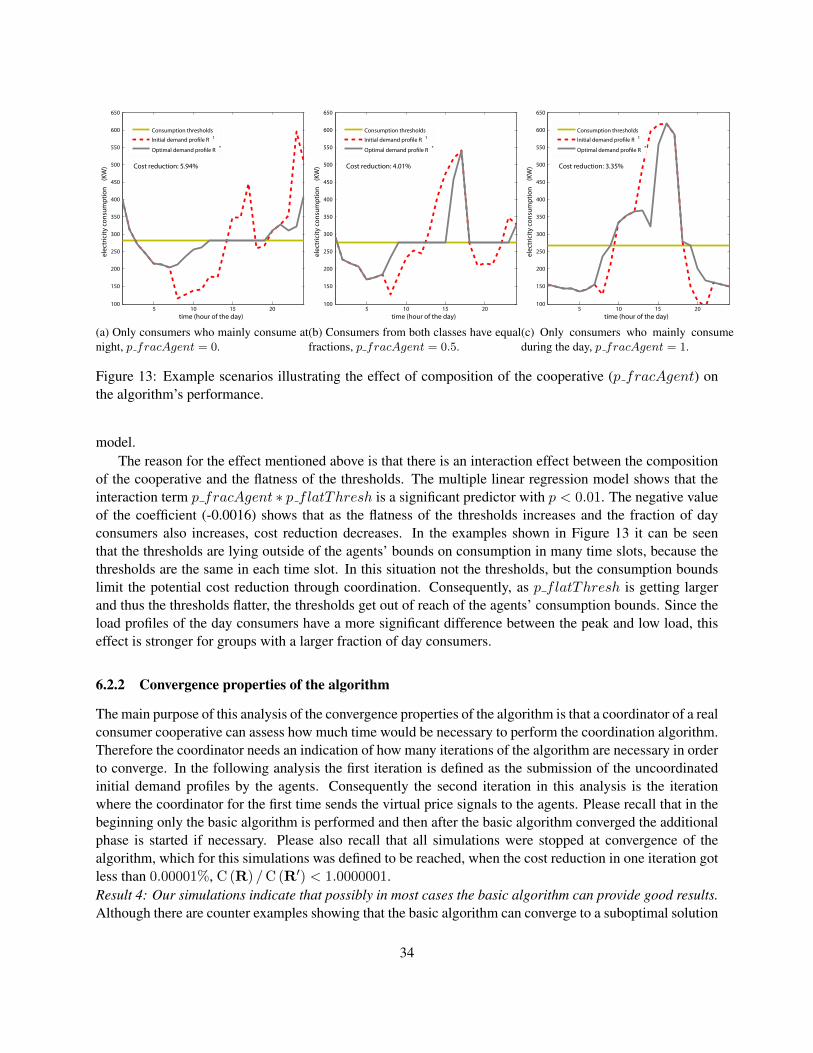
5 10 15 20100

150

200

250

300

350

400

450

500

550

600

650

time (hour of the day)

elec

tric

ity c

onsu

mpt

ion

(K

W)

Consumption thresholds

Initial demand pro�le R 1

Optimal demand pro�le R *

Cost reduction: 5.94%

(a) Only consumers who mainly consume atnight, p fracAgent = 0.

5 10 15 20100

150

200

250

300

350

400

450

500

550

600

650

time (hour of the day)el

ectr

icity

con

sum

ptio

n

(KW

)

Consumption thresholds

Initial demand pro�le R 1

Optimal demand pro�le R *

Cost reduction: 4.01%

(b) Consumers from both classes have equalfractions, p fracAgent = 0.5.

5 10 15 20100

150

200

250

300

350

400

450

500

550

600

650

time (hour of the day)

elec

tric

ity c

onsu

mpt

ion

(K

W)

Consumption thresholds

Initial demand pro�le R 1

Optimal demand pro�le R *

Cost reduction: 3.35%

(c) Only consumers who mainly consumeduring the day, p fracAgent = 1.

Figure 13: Example scenarios illustrating the effect of composition of the cooperative (p fracAgent) onthe algorithm’s performance.

model.The reason for the effect mentioned above is that there is an interaction effect between the composition

of the cooperative and the flatness of the thresholds. The multiple linear regression model shows that theinteraction term p fracAgent ∗ p flatThresh is a significant predictor with p < 0.01. The negative valueof the coefficient (-0.0016) shows that as the flatness of the thresholds increases and the fraction of dayconsumers also increases, cost reduction decreases. In the examples shown in Figure 13 it can be seenthat the thresholds are lying outside of the agents’ bounds on consumption in many time slots, because thethresholds are the same in each time slot. In this situation not the thresholds, but the consumption boundslimit the potential cost reduction through coordination. Consequently, as p flatThresh is getting largerand thus the thresholds flatter, the thresholds get out of reach of the agents’ consumption bounds. Since theload profiles of the day consumers have a more significant difference between the peak and low load, thiseffect is stronger for groups with a larger fraction of day consumers.

6.2.2 Convergence properties of the algorithm

The main purpose of this analysis of the convergence properties of the algorithm is that a coordinator of a realconsumer cooperative can assess how much time would be necessary to perform the coordination algorithm.Therefore the coordinator needs an indication of how many iterations of the algorithm are necessary in orderto converge. In the following analysis the first iteration is defined as the submission of the uncoordinatedinitial demand profiles by the agents. Consequently the second iteration in this analysis is the iterationwhere the coordinator for the first time sends the virtual price signals to the agents. Please recall that in thebeginning only the basic algorithm is performed and then after the basic algorithm converged the additionalphase is started if necessary. Please also recall that all simulations were stopped at convergence of thealgorithm, which for this simulations was defined to be reached, when the cost reduction in one iteration gotless than 0.00001%, C (R) /C (R′) < 1.0000001.Result 4: Our simulations indicate that possibly in most cases the basic algorithm can provide good results.Although there are counter examples showing that the basic algorithm can converge to a suboptimal solution

34

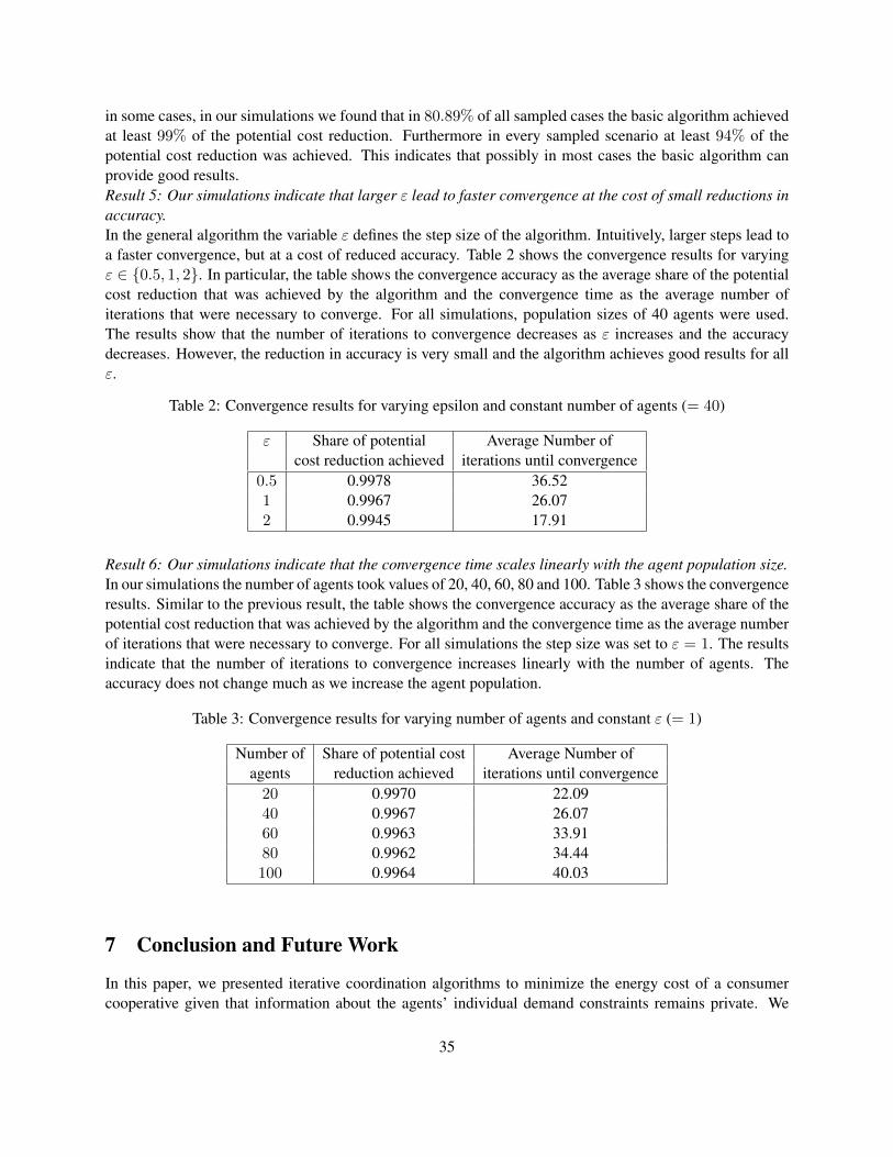
in some cases, in our simulations we found that in 80.89% of all sampled cases the basic algorithm achievedat least 99% of the potential cost reduction. Furthermore in every sampled scenario at least 94% of thepotential cost reduction was achieved. This indicates that possibly in most cases the basic algorithm canprovide good results.Result 5: Our simulations indicate that larger ε lead to faster convergence at the cost of small reductions inaccuracy.In the general algorithm the variable ε defines the step size of the algorithm. Intuitively, larger steps lead toa faster convergence, but at a cost of reduced accuracy. Table 2 shows the convergence results for varyingε ∈ {0.5, 1, 2}. In particular, the table shows the convergence accuracy as the average share of the potentialcost reduction that was achieved by the algorithm and the convergence time as the average number ofiterations that were necessary to converge. For all simulations, population sizes of 40 agents were used.The results show that the number of iterations to convergence decreases as ε increases and the accuracydecreases. However, the reduction in accuracy is very small and the algorithm achieves good results for allε.

Table 2: Convergence results for varying epsilon and constant number of agents (= 40)

ε Share of potential Average Number ofcost reduction achieved iterations until convergence

0.5 0.9978 36.521 0.9967 26.072 0.9945 17.91

Result 6: Our simulations indicate that the convergence time scales linearly with the agent population size.In our simulations the number of agents took values of 20, 40, 60, 80 and 100. Table 3 shows the convergenceresults. Similar to the previous result, the table shows the convergence accuracy as the average share of thepotential cost reduction that was achieved by the algorithm and the convergence time as the average numberof iterations that were necessary to converge. For all simulations the step size was set to ε = 1. The resultsindicate that the number of iterations to convergence increases linearly with the number of agents. Theaccuracy does not change much as we increase the agent population.

Table 3: Convergence results for varying number of agents and constant ε (= 1)

Number of Share of potential cost Average Number ofagents reduction achieved iterations until convergence

20 0.9970 22.0940 0.9967 26.0760 0.9963 33.9180 0.9962 34.44100 0.9964 40.03

7 Conclusion and Future Work

In this paper, we presented iterative coordination algorithms to minimize the energy cost of a consumercooperative given that information about the agents’ individual demand constraints remains private. We

35

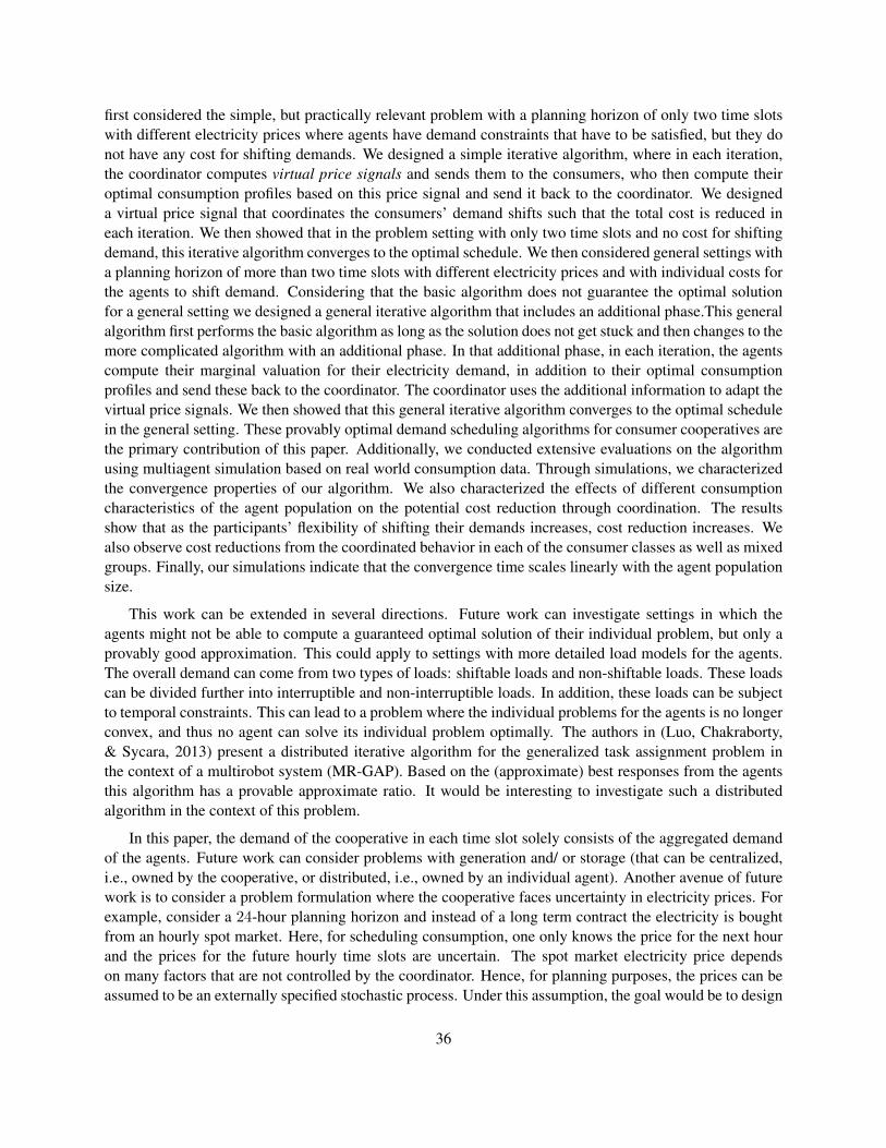
first considered the simple, but practically relevant problem with a planning horizon of only two time slotswith different electricity prices where agents have demand constraints that have to be satisfied, but they donot have any cost for shifting demands. We designed a simple iterative algorithm, where in each iteration,the coordinator computes virtual price signals and sends them to the consumers, who then compute theiroptimal consumption profiles based on this price signal and send it back to the coordinator. We designeda virtual price signal that coordinates the consumers’ demand shifts such that the total cost is reduced ineach iteration. We then showed that in the problem setting with only two time slots and no cost for shiftingdemand, this iterative algorithm converges to the optimal schedule. We then considered general settings witha planning horizon of more than two time slots with different electricity prices and with individual costs forthe agents to shift demand. Considering that the basic algorithm does not guarantee the optimal solutionfor a general setting we designed a general iterative algorithm that includes an additional phase.This generalalgorithm first performs the basic algorithm as long as the solution does not get stuck and then changes to themore complicated algorithm with an additional phase. In that additional phase, in each iteration, the agentscompute their marginal valuation for their electricity demand, in addition to their optimal consumptionprofiles and send these back to the coordinator. The coordinator uses the additional information to adapt thevirtual price signals. We then showed that this general iterative algorithm converges to the optimal schedulein the general setting. These provably optimal demand scheduling algorithms for consumer cooperatives arethe primary contribution of this paper. Additionally, we conducted extensive evaluations on the algorithmusing multiagent simulation based on real world consumption data. Through simulations, we characterizedthe convergence properties of our algorithm. We also characterized the effects of different consumptioncharacteristics of the agent population on the potential cost reduction through coordination. The resultsshow that as the participants’ flexibility of shifting their demands increases, cost reduction increases. Wealso observe cost reductions from the coordinated behavior in each of the consumer classes as well as mixedgroups. Finally, our simulations indicate that the convergence time scales linearly with the agent populationsize.

This work can be extended in several directions. Future work can investigate settings in which theagents might not be able to compute a guaranteed optimal solution of their individual problem, but only aprovably good approximation. This could apply to settings with more detailed load models for the agents.The overall demand can come from two types of loads: shiftable loads and non-shiftable loads. These loadscan be divided further into interruptible and non-interruptible loads. In addition, these loads can be subjectto temporal constraints. This can lead to a problem where the individual problems for the agents is no longerconvex, and thus no agent can solve its individual problem optimally. The authors in (Luo, Chakraborty,& Sycara, 2013) present a distributed iterative algorithm for the generalized task assignment problem inthe context of a multirobot system (MR-GAP). Based on the (approximate) best responses from the agentsthis algorithm has a provable approximate ratio. It would be interesting to investigate such a distributedalgorithm in the context of this problem.

In this paper, the demand of the cooperative in each time slot solely consists of the aggregated demandof the agents. Future work can consider problems with generation and/ or storage (that can be centralized,i.e., owned by the cooperative, or distributed, i.e., owned by an individual agent). Another avenue of futurework is to consider a problem formulation where the cooperative faces uncertainty in electricity prices. Forexample, consider a 24-hour planning horizon and instead of a long term contract the electricity is boughtfrom an hourly spot market. Here, for scheduling consumption, one only knows the price for the next hourand the prices for the future hourly time slots are uncertain. The spot market electricity price dependson many factors that are not controlled by the coordinator. Hence, for planning purposes, the prices can beassumed to be an externally specified stochastic process. Under this assumption, the goal would be to design

36

algorithms for (1) determining policies (for generation, storage, and price signals to be sent to the firms) forthe central coordinator and (2) determine the schedules for the individual firms, such that the expected costof buying electricity is minimized.

Acknowledgements

This work was partially supported by NSF award IIS-1218542.

References

Albadi, M., & El-Saadany, E. (2007). Demand response in electricity markets: An overview. In PowerEngineering Society General Meeting, 2007. IEEE, pp. 1–5. IEEE.

Atzeni, I., Ordonez, L., Scutari, G., Palomar, D., & Fonollosa, J. (2013). Demand-side management viadistributed energy generation and storage optimization. Smart Grid, IEEE Transactions on, 4(2),866–876.

Baharlouei, Z., Hashemi, M., Narimani, H., & Mohsenian-Rad, H. (2013). Achieving optimality and fairnessin autonomous demand response: Benchmarks and billing mechanisms. Smart Grid, IEEE Transac-tions on, 4(2), 968–975.

Bertsekas, D. P., & Tsitsiklis, J. N. (1989). Parallel and distributed computation: numerical methods.Prentice-Hall, Inc., Upper Saddle River, NJ, USA.

Boyd, S., & Vandenberghe, L. (2004). Convex optimization. Cambridge university press.

Chu, C., & Jong, T. (2008). A novel direct air-conditioning load control method. Power Systems, IEEETransactions on, 23(3), 1356–1363.

Clement-Nyns, K., Haesen, E., & Driesen, J. (2010). The impact of charging plug-in hybrid electric vehicleson a residential distribution grid. Power Systems, IEEE Transactions on, 25(1), 371–380.

Conejo, A., Morales, J., & Baringo, L. (2010). Real-time demand response model. Smart Grid, IEEETransactions on, 1(3), 236–242.

Dietrich, K., Latorre, J., Olmos, L., & Ramos, A. (2012). Demand response in an isolated system with highwind integration. Power Systems, IEEE Transactions on, 27(1), 20–29.

DOE, U. (2003). Grid 2030: A national vision for electricity’s second 100 years..

Jellings, C. W., & Chamberlin, J. H. (1993). Demand Side Management: Concepts and Methods. PennWellBooks, Tulsa, OK.

Kim, T., & Poor, H. (2011). Scheduling power consumption with price uncertainty. Smart Grid, IEEETransactions on, 2(3), 519–527.

Kirschen, D. (2003). Demand-side view of electricity markets. Power Systems, IEEE Transactions on,18(2), 520–527.

Luo, L., Chakraborty, N., & Sycara, K. (2013). Distributed algorithm design for multi-robot generalized taskassignment. In Proceedings of IEEE International Conference on Intelligent Robots and Systems.

Medina, J., Muller, N., & Roytelman, I. (2010). Demand response and distribution grid operations: Oppor-tunities and challenges. Smart Grid, IEEE Transactions on, 1(2), 193–198.

37

Mohsenian-Rad, A., Wong, V., Jatskevich, J., Schober, R., & Leon-Garcia, A. (2010). Autonomous demand-side management based on game-theoretic energy consumption scheduling for the future smart grid.Smart Grid, IEEE Transactions on, 1(3), 320–331.

Mohsenian-Rad, A., & Leon-Garcia, A. (2010). Optimal residential load control with price prediction inreal-time electricity pricing environments. Smart Grid, IEEE Transactions on, 1(2), 120–133.

Nguyen, H. K., Song, J. B., & Han, Z. (2012). Demand side management to reduce peak-to-average ratiousing game theory in smart grid. In Computer Communications Workshops (INFOCOM WKSHPS),2012 IEEE Conference on, pp. 91–96. IEEE.

Palensky, P., & Dietrich, D. (2011). Demand side management: Demand response, intelligent energy sys-tems, and smart loads. Industrial Informatics, IEEE Transactions on, 7(3), 381–388.

Parvania, M., & Fotuhi-Firuzabad, M. (2010). Demand response scheduling by stochastic scuc. Smart Grid,IEEE Transactions on, 1(1), 89–98.

Pedrasa, M., Spooner, T., & MacGill, I. (2010). Coordinated scheduling of residential distributed energyresources to optimize smart home energy services. Smart Grid, IEEE Transactions on, 1(2), 134–143.

Philpott, A., & Pettersen, E. (2006). Optimizing demand-side bids in day-ahead electricity markets. PowerSystems, IEEE Transactions on, 21(2), 488–498.

Rahimi, F., & Ipakchi, A. (2010). Demand response as a market resource under the smart grid paradigm.IEEE Transactions on Smart Grid, 1(1), 82–88.

Ramchurn, S., Vytelingum, P., Rogers, A., & Jennings, N. (2012). Putting the ’smarts’ into the smart grid:A grand challenge for artificial intelligence. Communications of the ACM, 55(4), 86–97.

Ramchurn, S. D., Vytelingum, P., Rogers, A., & Jennings, N. (2011). Agent-based control for decentraliseddemand side management in the smart grid. In The 10th International Conference on AutonomousAgents and Multiagent Systems-Volume 1, pp. 5–12.

Samadi, P., Mohsenian-Rad, H., Wong, V., & Schober, R. (2013). Tackling the load uncertainty challengesfor energy consumption scheduling in smart grid. Smart Grid, IEEE Transactions on, 4(2), 1007–1016.

Tanaka, K., Uchida, K., Ogimi, K., Goya, T., Yona, A., Senjy, T., Funabashi, T., & Kim, C. (2011). Optimaloperation by controllable loads based on smart grid topology considering insolation forecasted error.Smart Grid, IEEE Transactions on, 2(3), 438–444.

Veit, A., Xu, Y., Zheng, R., Chakraborty, N., & Sycara, K. (2013). Multiagent coordination for energy con-sumption scheduling in consumer cooperatives. In Proceedings of 27th AAAI Conference on ArtificialIntelligence.

Voice, T., Vytelingum, P., Ramchurn, S., Rogers, A., & Jennings, N. (2011). Decentralised control of micro-storage in the smart grid. In AAAI Conference on Artificial Intelligence.

Vytelingum, P., Ramchurn, S., Rogers, A., & Jennings, N. (2010). Agent-based homeostatic control forgreen energy in the smart grid. In First International Workshop on Agent Technologies for EnergySystems (ATES 2010).

Vytelingum, P., Voice, T., Ramchurn, S., Rogers, A., & Jennings, N. (2011). Theoretical and practical foun-dations of large-scale agent-based micro-storage in the smart grid. Journal of Artificial IntelligenceResearch, 42(1), 765–813.

38

Wood, A., & Wollenberg, B. (1996). Power Generation Operation and Control. John Wiley & Sons.

Wu, C., Mohsenian-Rad, H., & Huang, J. (2012). Wind power integration via aggregator-consumer coordi-nation: A game theoretic approach. In Innovative Smart Grid Technologies (ISGT), 2012 IEEE PES,pp. 1–6. IEEE.

Wu, C., Mohsenian-Rad, H., Huang, J., & Wang, A. Y. (2011). Demand side management for wind powerintegration in microgrid using dynamic potential game theory. In GLOBECOM Workshops (GC Wk-shps), 2011 IEEE, pp. 1199–1204. IEEE.

Appendix

A Proof: Virtual cost is an upper bound on the total cost

Proof. Here we give the full algebraic proof showing that the sum of the agents’ individual cost accordingto their virtual price signals is an upper bound on the total central cost at market prices. We prove this byshowing with Equations (1) and (7) that for every time slot j the difference between the total cost for theaggregated demand and the sum of the agents’ individual cost is lower or equal to 0. Since it is true for everytime slot it is also true for the sum over all time slots.

The central cost for the aggregated demand is given in Equation (1) as

N∑i=1

pj

(ρ′j)r′ij , ∀j

= pHj(ρ′j − hj

)++ pLj

(ρ′j − hj

)−+ pLj hj

=

pHj

(ρ′j − hj

)+ pLj hj ρ′j > hj

pLj

(ρ′j − hj

)+ pLj hj ρ′j ≤ hj

=

∑N

i=1

(pHj

(r′ij − hij

))+∑N

i=1

(pLj hij

)ρ′j > hj∑N

i=1

(pLj

(r′ij − hij

))+∑N

i=1

(pLj hij

)ρ′j ≤ hj

The sum of the agents’ individual cost is given in Equation (7) as

N∑i=1

sij(r′ij)r′ij , ∀j

=N∑i=1

[pHj(r′ij − hij

)++ pLj

(r′ij − hij

)−+ pLj hij

]For the difference of the two costs we get:

N∑i=1

pj

(ρ′j)r′ij −

N∑i=1

sij(r′ij)r′ij , ∀j

=

∑N

i=1

[pHj

(r′ij − hij

)+ pLj hij − pHj

(r′ij − hij

)+− pLj

(r′ij − hij

)−− pLj hij

]ρ′j > hj∑N

i=1

[pLj

(r′ij − hij

)+ pLj hij − pHj

(r′ij − hij

)+− pLj

(r′ij − hij

)−− pLj hij

]ρ′j ≤ hj

39

Since∑N

i=1

(pLj hij

)and −

∑Ni=1

(pLj hij

)equal each other out they and can be removed.

=

∑N

i=1

[pHj

(r′ij − hij

)− pHj

(r′ij − hij

)+− pLj

(r′ij − hij

)−]ρ′j > hj∑N

i=1

[pLj

(r′ij − hij

)− pHj

(r′ij − hij

)+− pLj

(r′ij − hij

)−]ρ′j ≤ hj

Lets now write∑N

i=1 pHj

(r′ij − hij

)+as∑N

i: r′ij>hijpHj

(r′ij − hij

)and

∑Ni=1 p

Lj

(r′ij − hij

)−analog as∑N

i: r′ij≤hijpHj

(r′ij − hij

). Lets also write

∑Ni=1 as

∑Ni: r′ij>hij

+∑N

i: r′ij≤hij.

=

{∑Ni: r′ij>hij

[pHj(r′ij − hij

)− pHj

(r′ij − hij

)]+∑N

i: r′ij≤hij

[pHj(r′ij − hij

)− pLj

(r′ij − hij

)]ρ′j > hj∑N

i: r′ij>hij

[pLj(r′ij − hij

)− pHj

(r′ij − hij

)]+∑N

i: r′ij≤hij

[pLj(r′ij − hij

)− pLj

(r′ij − hij

)]ρ′j ≤ hj

For ρ′j > hj the terms∑N

i: r′ij>hijpHj

(r′ij − hij

)and −

∑Ni: r′ij>hij

pHj

(r′ij − hij

)equal each other out

and can be removed. For ρ′j ≤ hj remove∑N

i: r′ij≤hijpLj

(r′ij − hij

)respectively.

=

∑N

i: r′ij≤hij

[pHj

(r′ij − hij

)− pLj

(r′ij − hij

)]ρ′j > hj∑N

i: r′ij>hij

[pLj

(r′ij − hij

)− pHj

(r′ij − hij

)]ρ′j ≤ hj

Factor(pHj − pLj

)and

(pLj − pHj

)out.

=

∑N

i: r′ij≤hij

(pHj − pLj

)(r′ij − hij

)ρ′j > hj∑N

i: r′ij>hij

(pLj − pHj

)(r′ij − hij

)ρ′j ≤ hj

=

∑N

i=1

(pHj − pLj

)(r′ij − hij

)−ρ′j > hj∑N

i=1

(pLj − pHj

)(r′ij − hij

)+ρ′j ≤ hj

=

[∑N

i=1

(pHj − pLj

)(r′ij − hij

)−]≤ 0 ρ′j > hj[∑N

i=1

(pLj − pHj

)(r′ij − hij

)+]≤ 0 ρ′j ≤ hj

Since this inequality is true for every time slot, it also holds for the sum over all time slots. It follows thatthe sum of the agents’ individual cost according to their virtual price signals is an upper bound on the totalcentral cost at market prices, C (R′) ≤

∑Ni=1 Ci (r′i):

N∑i=1

M∑j=1

pj

(ρ′j)r′ij + gi(r

′i) ≤

N∑i=1

M∑j=1

sij(r′ij)r′ij + gi(r

′i)

40

B Proof by counterexample: Basic algorithm can converge to a suboptimalsolution in case of gi(·) 6= 0

We present a counterexample to prove that the basic algorithm can converge to a suboptimal solution ingeneral settings with gi(·) 6= 0. Consider a population of 2 agents, N = 2, and a planning horizon of 2 timeslots, M = 2. The agents’ constraints are such that in the converged solution, the aggregated demand isequal to the threshold in one time slot. Let the price function for the two time slots be given as:

(pL1 , pH1 ) = (3, 8), h1 = 9

(pL2 , pH2 ) = (3, 8), h2 = 11

The individual constraints on the agents’ consumption are:

r11 ∈ [1, 3], r12 ∈ [4, 6], r11 + r12 = τ1 = 7

r21 ∈ [4, 6], r22 ∈ [4, 6], r21 + r22 = τ2 = 10

In addition to the electricity cost the two agents have to consider additional cost associated with the demandschedule. This additional cost for is given as:

g1 (r1) = r1

[51

], g2 (r2) = r2

[63

]Let R(t) denote the demand profile of the agents in the tth iteration and let t = 1 be the initial demandprofile. At the beginning the agents compute their initial demand profiles based on the market prices r(1)

1 =

(1, 6), r(1)2 = (4, 6). The cost based on the initial demand profiles is C

(R(1)

)= 109. Subsequently, the

coordinator computes the thresholds for the virtual price signals by comparing the initial demand profiles tothe thresholds of the price function. The thresholds for the virtual price signals are

h11(R(1)) = 1.8, h12(R(1)) = 5.5

h21(R(1)) = 7.2, h22(R(1)) = 5.5

Based on the virtual price signals the agents compute their next demand profiles r(2)1 = (1.5, 5.5), r(2)

2 =(4.5, 5.5). The cost based on this next demand profiles is C

(R(2)

)= 107.5. Subsequently the coordinator

computes the thresholds for the new virtual price signals

h11(R(2)) = 2.25, h12(R(2)) = 5.5

h21(R(2)) = 6.75, h22(R(2)) = 5.5

Since no agent can improve its cost given this virtual price signal the demand profiles keep unchanged sothat R(T ) = R(2). Thus, the algorithm ends. However a different demand profile of the agents, r′1 = (1, 6),r′2 = (5, 5), is feasible and leads to lower total cost C (R′) = 107. It follows that the algorithm has stoppedin a suboptimal solution.

41