Demand Side Management Concept, Options and Program Design

Rangan Banerjee

Forbes Marshall Chair Professor

Department of Energy Science and Engineering

Indian Institute of Technology Bombay

Presentation at DSM Workshop 4th April 2014 Lucknow

Demand Side Management

Indian utilities – energy shortage and peak power shortage.

Supply Focussed- Build New Power Plants.

Capital & Fuel Scarcity, Environmental Impacts, Gestation Period.

Need for Options – Demand Side Management (DSM) & Load Management

DSM Concept

Demand Side Management (DSM) - co-operative action by the customer & the utility(SEB) to modify the customer load

DSM benefits utility, consumer & society

Energy Conservation

Fuel Switching

Peak Clipping/Valley Filling/Load Shifting

Electric Utility Role

Provision of Electricity to customers in the service area- supply customers with power they wish at whatever time

Planning under uncertainty of demand

Daily, Weekly & Seasonal Load Variation

Conventional power planning -Demand – exogenous, uncontrollable – build new supply to meet demand

Redefining Role

Capacity additions costly – Shortages of peak power and energy

Low capacity utilisation of power plants – increased costs – high tariffs

Gestation Period

Provision of energy services(using electricity) to customers in the service area (lighting, cooling, motive power…)

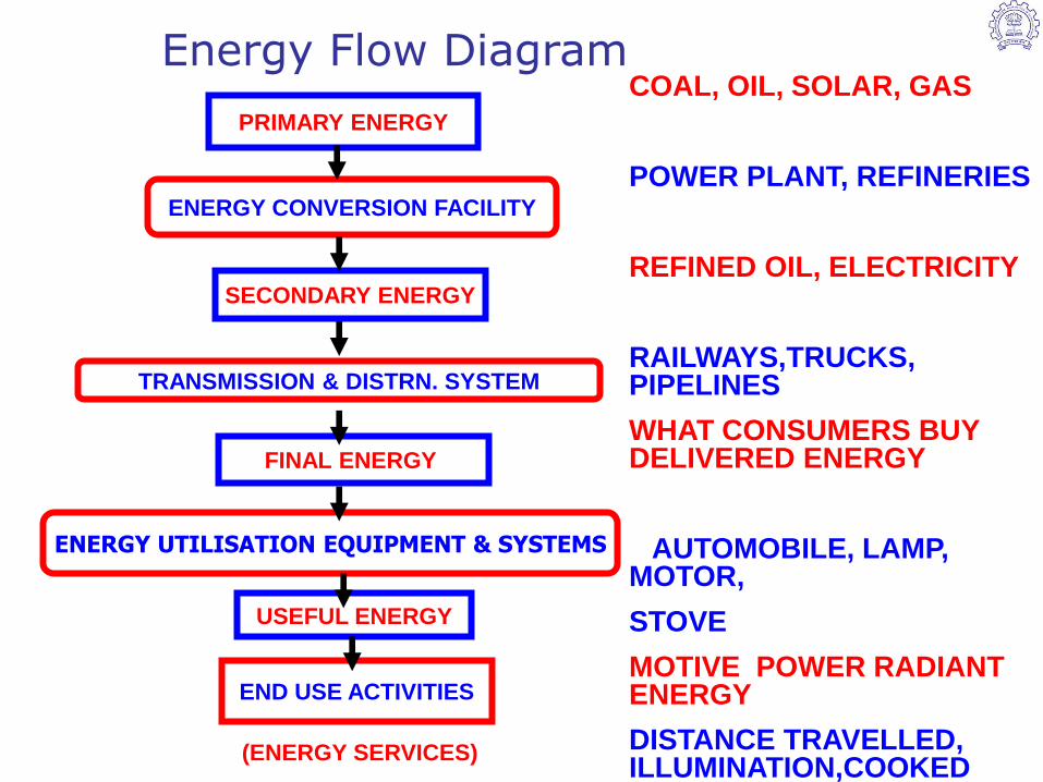
Energy Flow Diagram

PRIMARY ENERGY

ENERGY CONVERSION FACILITY

SECONDARY ENERGY

TRANSMISSION & DISTRN. SYSTEM

FINAL ENERGY

ENERGY UTILISATION EQUIPMENT & SYSTEMS

USEFUL ENERGY

END USE ACTIVITIES

(ENERGY SERVICES)

COAL, OIL, SOLAR, GAS

POWER PLANT, REFINERIES

REFINED OIL, ELECTRICITY

RAILWAYS,TRUCKS, PIPELINES

WHAT CONSUMERS BUY DELIVERED ENERGY

AUTOMOBILE, LAMP, MOTOR,

STOVE

MOTIVE POWER RADIANT ENERGY

DISTANCE TRAVELLED, ILLUMINATION,COOKED FOOD etc..

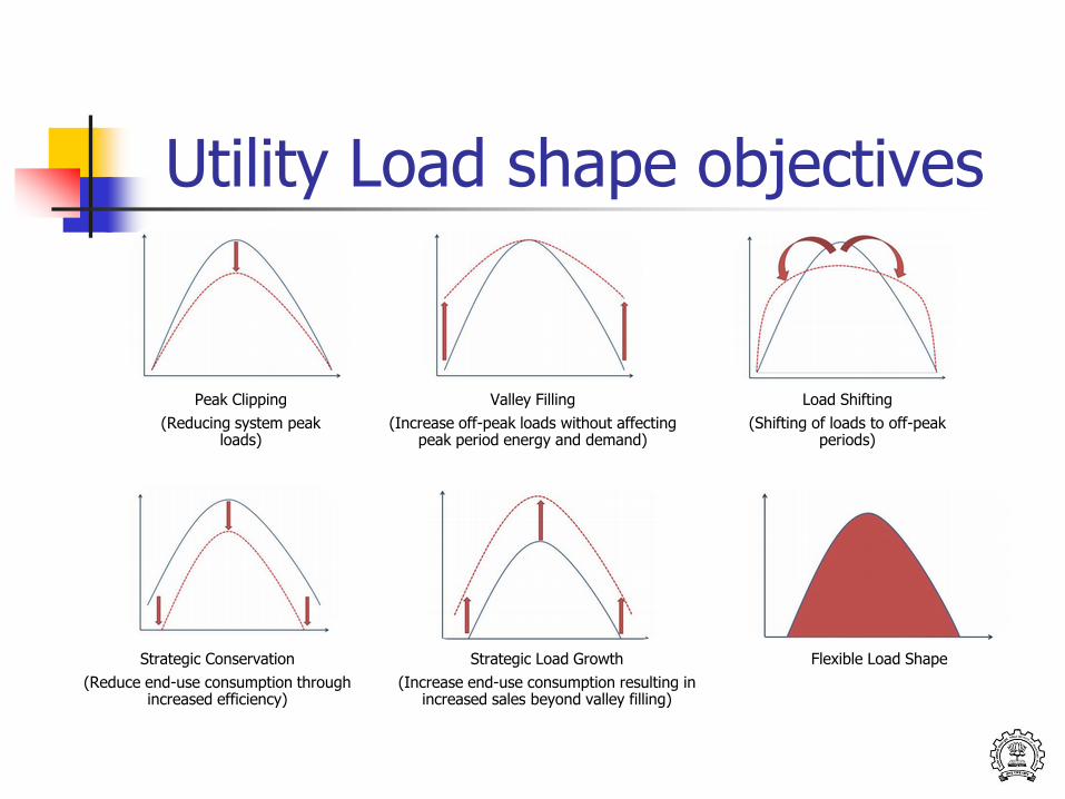
Utility Load shape objectives

Peak Clipping

(Reducing system peak loads)

Valley Filling

(Increase off-peak loads without affecting peak period energy and demand)

Load Shifting

(Shifting of loads to off-peak periods)

Strategic Conservation

(Reduce end-use consumption through increased efficiency)

Strategic Load Growth

(Increase end-use consumption resulting in increased sales beyond valley filling)

Flexible Load Shape

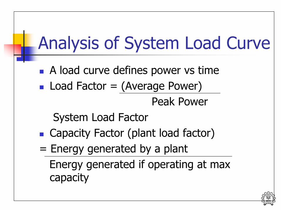
Analysis of System Load Curve

A load curve defines power vs time

Load Factor = (Average Power)

Peak Power

System Load Factor

Capacity Factor (plant load factor)

= Energy generated by a plant

Energy generated if operating at max capacity

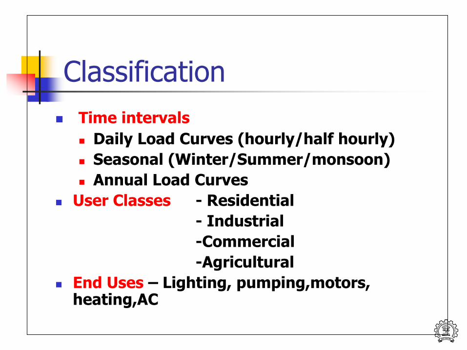
Classification

Time intervals

Daily Load Curves (hourly/half hourly)

Seasonal (Winter/Summer/monsoon)

Annual Load Curves

User Classes - Residential

- Industrial

-Commercial

-Agricultural

End Uses – Lighting, pumping,motors, heating,AC

Load Duration Curve

Frequency Distribution of loads

Re-arrange data to obtain cumulative number of hours where demand specified value

Plot – Load Duration curve

Highest load period -15-20% of the hours- designated as peak

Base Load – present for 70-80% of time

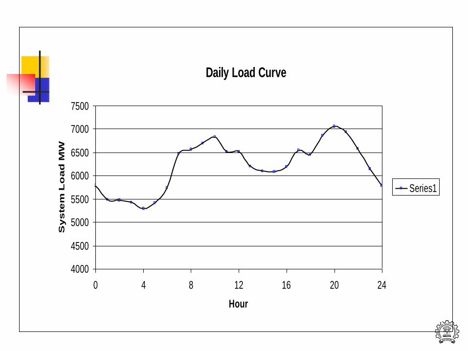
Daily Load Curve

4000

4500

5000

5500

6000

6500

7000

7500

0 4 8 12 16 20 24

Hour

Sy

ste

m L

oa

d M

W

Series1

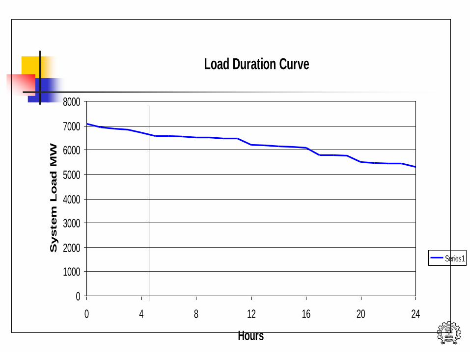
Load Duration Curve

0

1000

2000

3000

4000

5000

6000

7000

8000

0 4 8 12 16 20 24

Hours

System

Lo

ad

MW

Series1

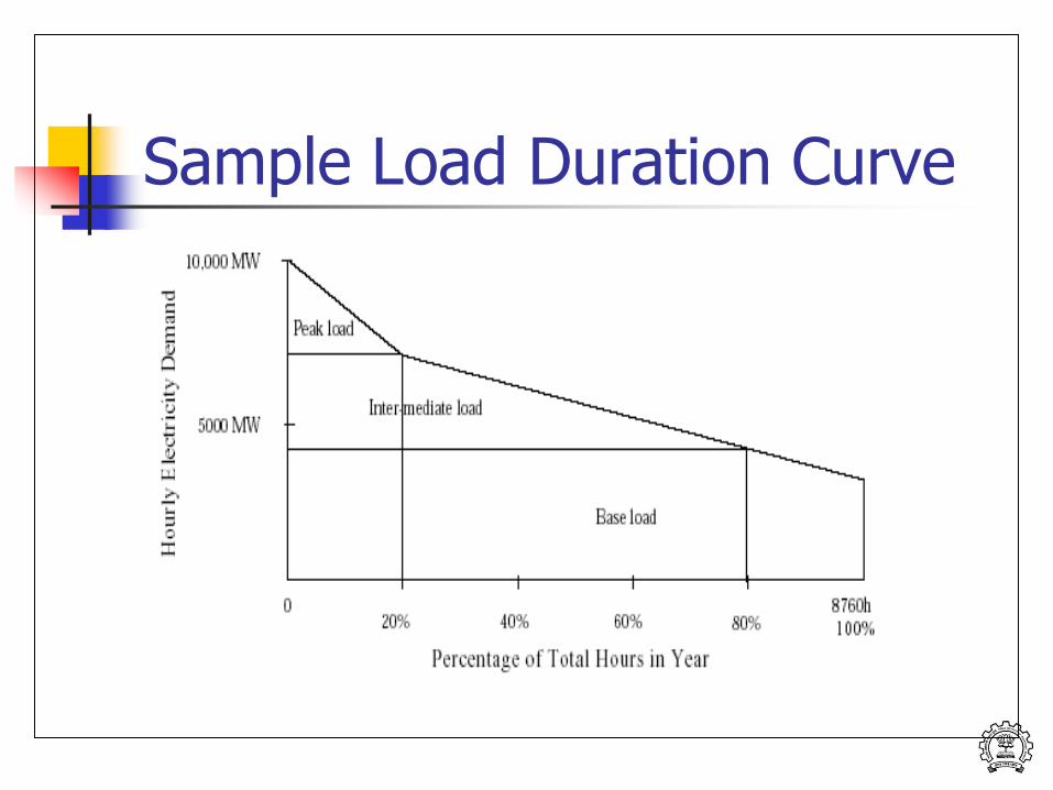
Sample Load Duration Curve

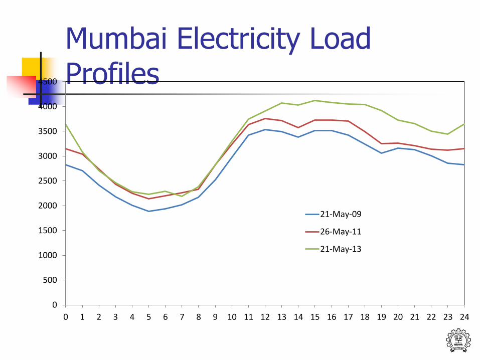
Mumbai Electricity Load Profiles

0

500

1000

1500

2000

2500

3000

3500

4000

4500

0 1 2 3 4 5 6 7 8 9 10 11 12 13 14 15 16 17 18 19 20 21 22 23 24

21-May-09

26-May-11

21-May-13

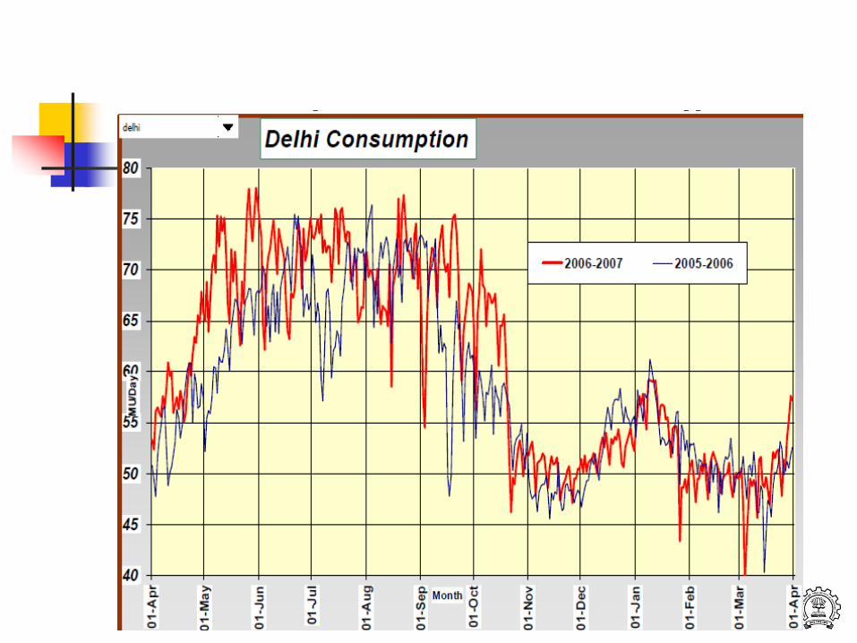
Seasonal Variations - Delhi

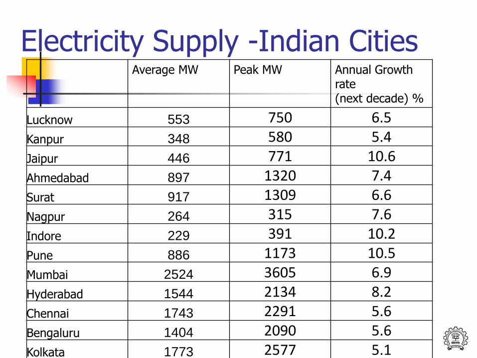
Electricity Supply -Indian Cities Average MW Peak MW Annual Growth

rate (next decade) %

Lucknow 553 750 6.5

Kanpur 348 580 5.4

Jaipur 446 771 10.6

Ahmedabad 897 1320 7.4

Surat 917 1309 6.6

Nagpur 264 315 7.6

Indore 229 391 10.2

Pune 886 1173 10.5

Mumbai 2524 3605 6.9

Hyderabad 1544 2134 8.2

Chennai 1743 2291 5.6

Bengaluru 1404 2090 5.6

Kolkata 1773 2577 5.1

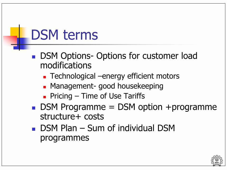
DSM terms

DSM Options- Options for customer load modifications Technological –energy efficient motors

Management- good housekeeping

Pricing – Time of Use Tariffs

DSM Programme = DSM option +programme structure+ costs

DSM Plan – Sum of individual DSM programmes

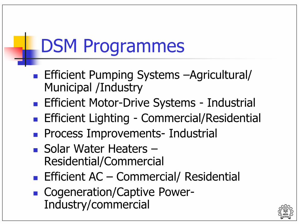
DSM Programmes

Efficient Pumping Systems –Agricultural/ Municipal /Industry

Efficient Motor-Drive Systems - Industrial

Efficient Lighting - Commercial/Residential

Process Improvements- Industrial

Solar Water Heaters –Residential/Commercial

Efficient AC – Commercial/ Residential

Cogeneration/Captive Power- Industry/commercial

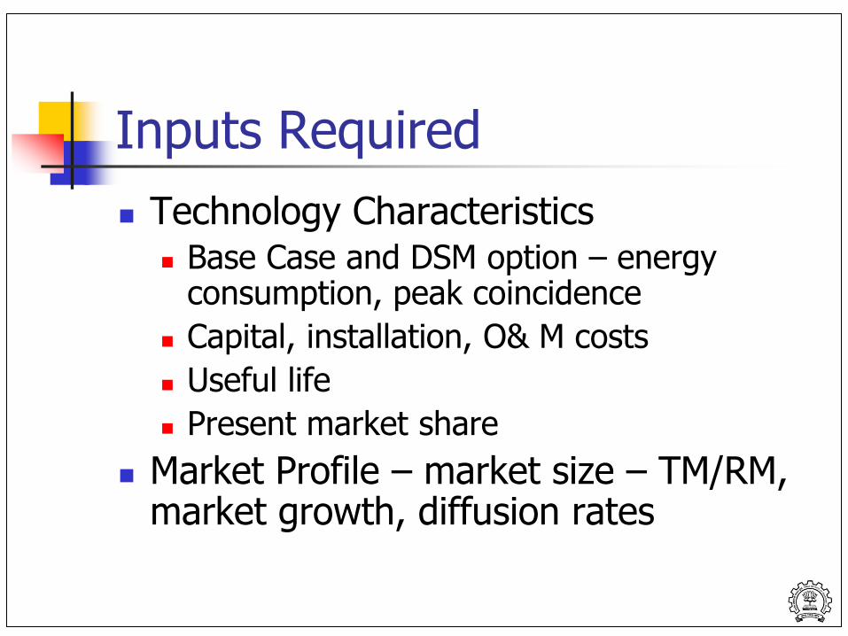
Inputs Required

Technology Characteristics Base Case and DSM option – energy

consumption, peak coincidence

Capital, installation, O& M costs

Useful life

Present market share

Market Profile – market size – TM/RM, market growth, diffusion rates

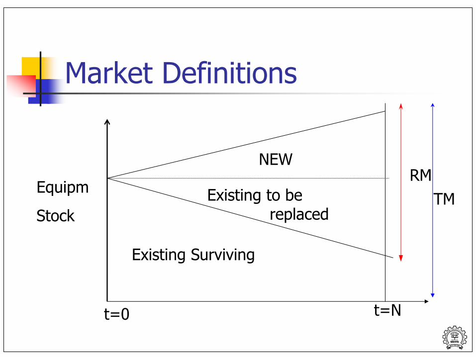
Market Definitions

t=0 t=N

Equipm

Stock

NEW

Existing to be replaced

RM

TM

Existing Surviving

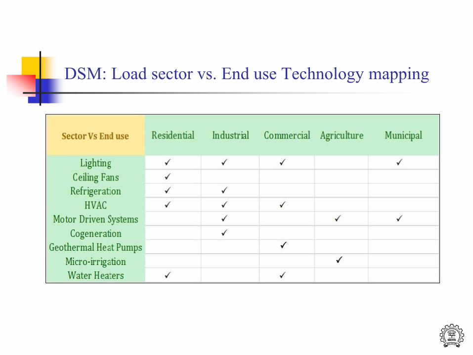
DSM: Load sector vs. End use Technology mapping

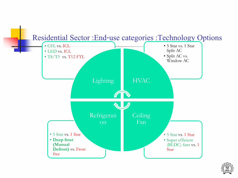
Residential Sector :End-use categories :Technology Options

• 5 Star vs. 1 Star

• Super efficient (BLDC) fans vs. 1 Star

• 5 Star vs. 1 Star

• Deep frost (Manual Defrost) vs. Frost free

• 5 Star vs. 1 Star Split AC

• Split AC vs. Window AC

• CFL vs. ICL

• LED vs. ICL

• T8/T5 vs. T12 FTL

Lighting HVAC

Ceiling Fan

Refrigeration

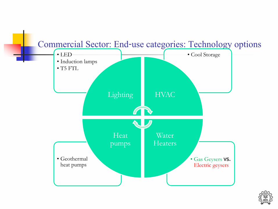
Commercial Sector: End-use categories: Technology options

• Gas Geysers vs. Electric geysers

• Geothermal heat pumps

• Cool Storage

• LED

• Induction lamps

• T5 FTL

Lighting HVAC

Water Heaters

Heat pumps

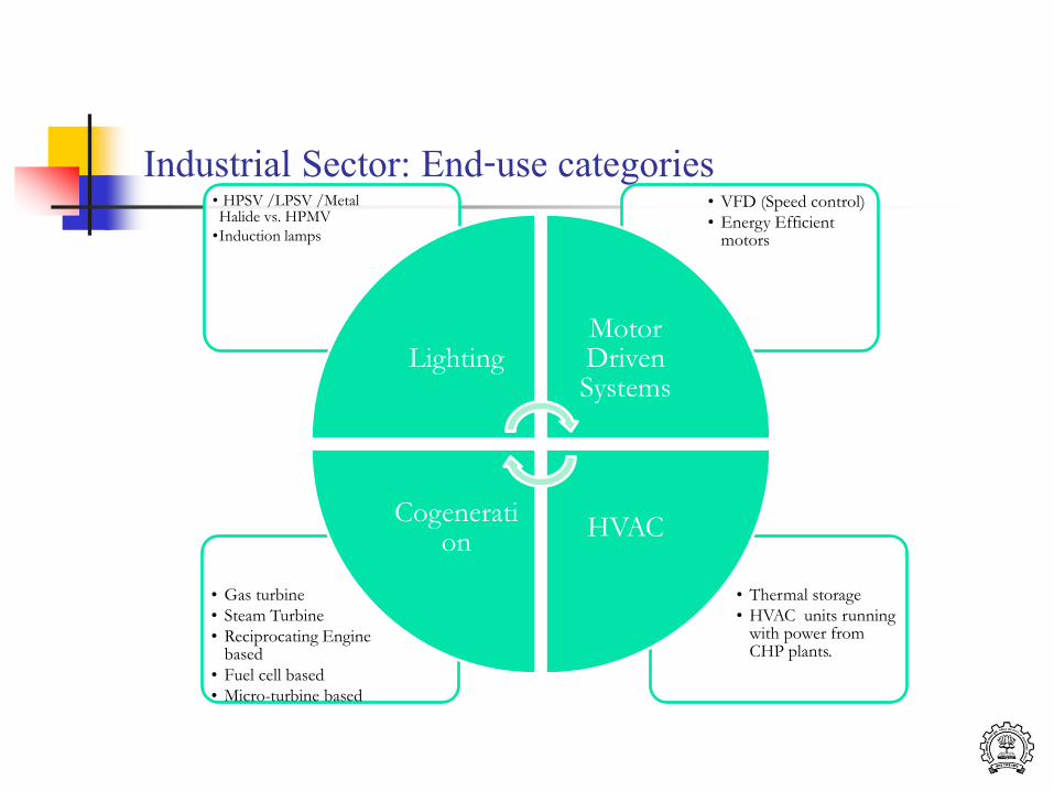
Industrial Sector: End-use categories

• Thermal storage

• HVAC units running with power from CHP plants.

• Gas turbine

• Steam Turbine

• Reciprocating Engine based

• Fuel cell based

• Micro-turbine based

• VFD (Speed control)

• Energy Efficient motors

• HPSV /LPSV /Metal Halide vs. HPMV

•Induction lamps

Lighting Motor Driven Systems

HVAC Cogenerati

on

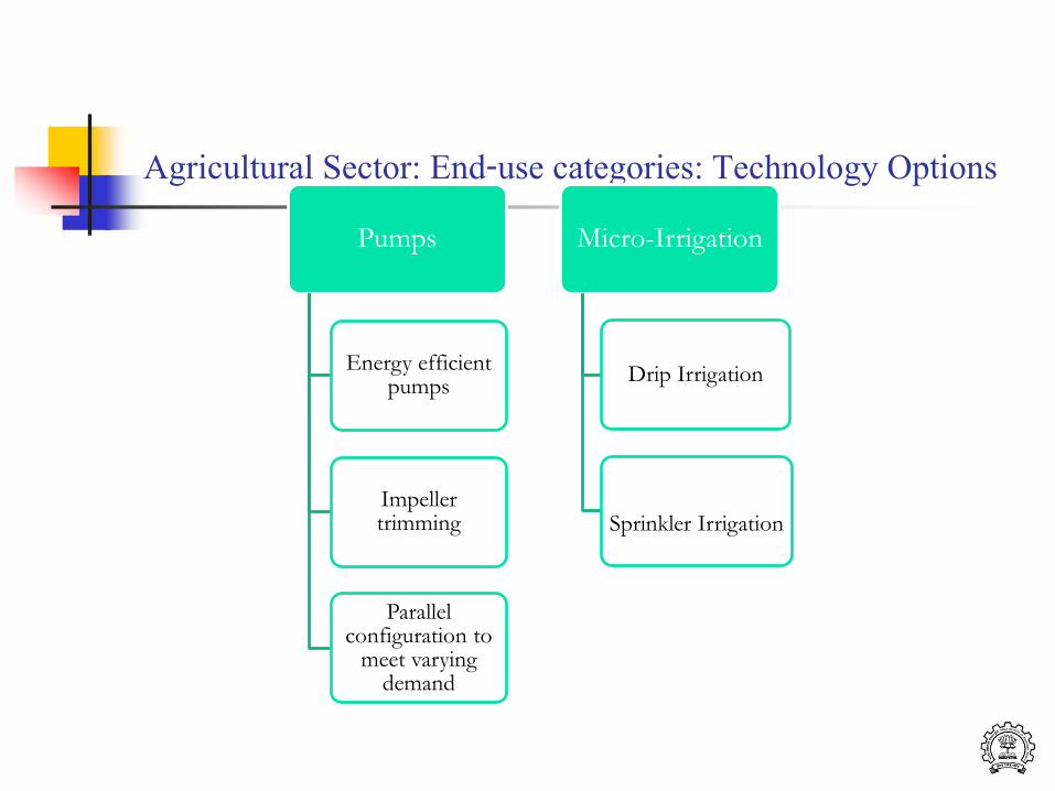
Agricultural Sector: End-use categories: Technology Options Pumps

Energy efficient pumps

Impeller trimming

Parallel configuration to

meet varying demand

Micro-Irrigation

Drip Irrigation

Sprinkler Irrigation

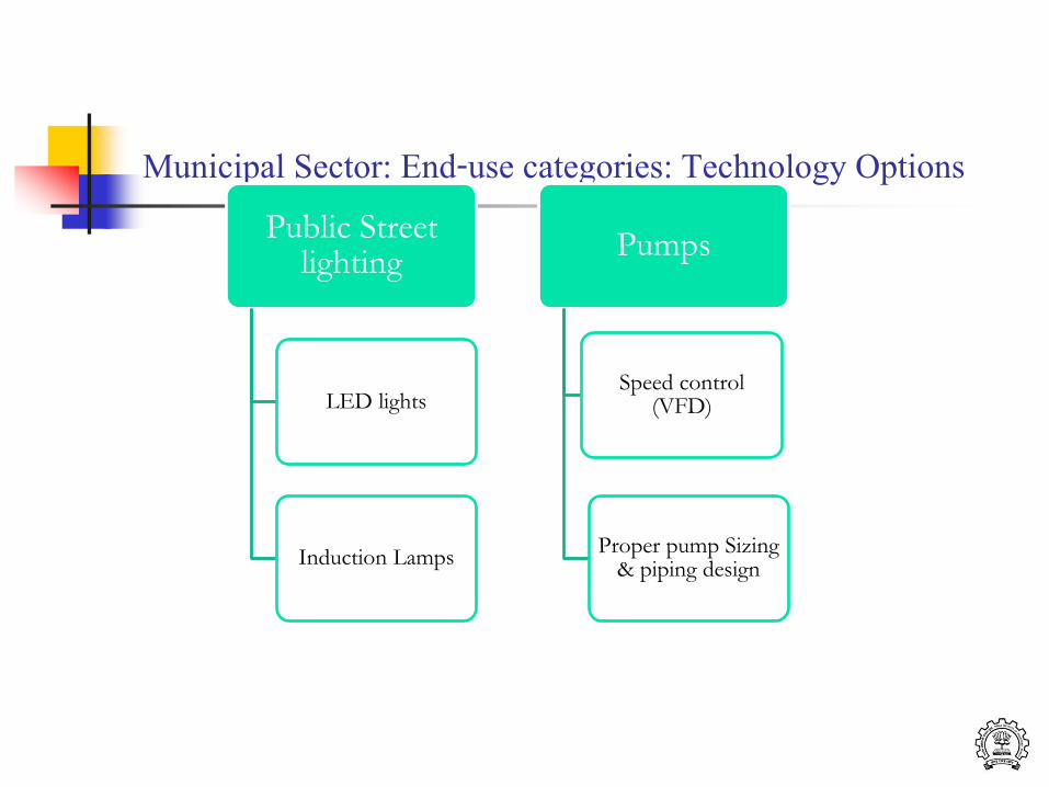
Municipal Sector: End-use categories: Technology Options Public Street

lighting

LED lights

Induction Lamps

Pumps

Speed control (VFD)

Proper pump Sizing & piping design

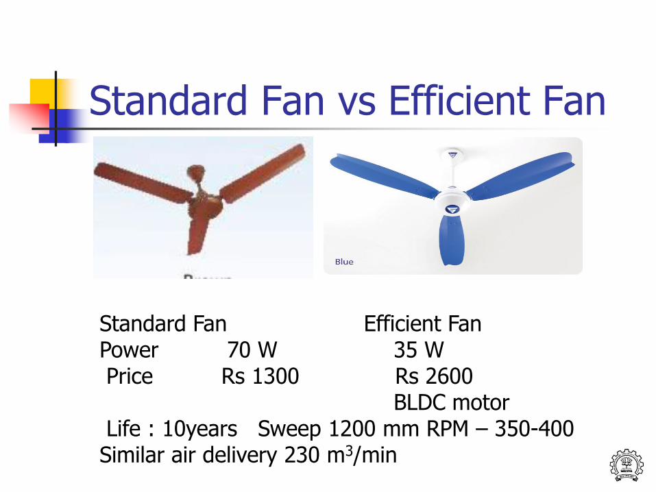
Standard Fan vs Efficient Fan

27

Standard Fan Efficient Fan Power 70 W 35 W Price Rs 1300 Rs 2600 BLDC motor Life : 10years Sweep 1200 mm RPM – 350-400 Similar air delivery 230 m3/min

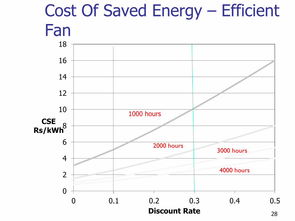
Cost Of Saved Energy – Efficient Fan

28

0

2

4

6

8

10

12

14

16

18

0 0.1 0.2 0.3 0.4 0.5

CSE Rs/kWh

Discount Rate

1000 hours

2000 hours

4000 hours

3000 hours

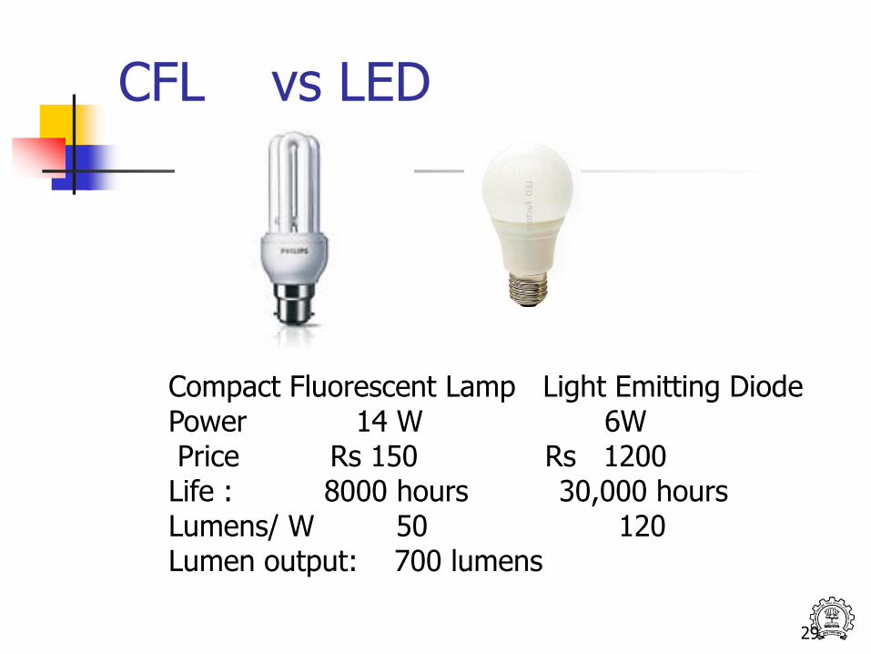
CFL vs LED

29

Compact Fluorescent Lamp Light Emitting Diode Power 14 W 6W Price Rs 150 Rs 1200 Life : 8000 hours 30,000 hours Lumens/ W 50 120 Lumen output: 700 lumens

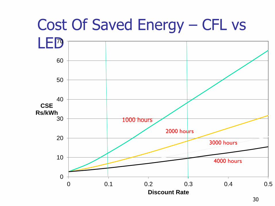
Cost Of Saved Energy – CFL vs LED

30

0

10

20

30

40

50

60

70

0 0.1 0.2 0.3 0.4 0.5

CSE Rs/kWh

Discount Rate

1000 hours

2000 hours

4000 hours

3000 hours

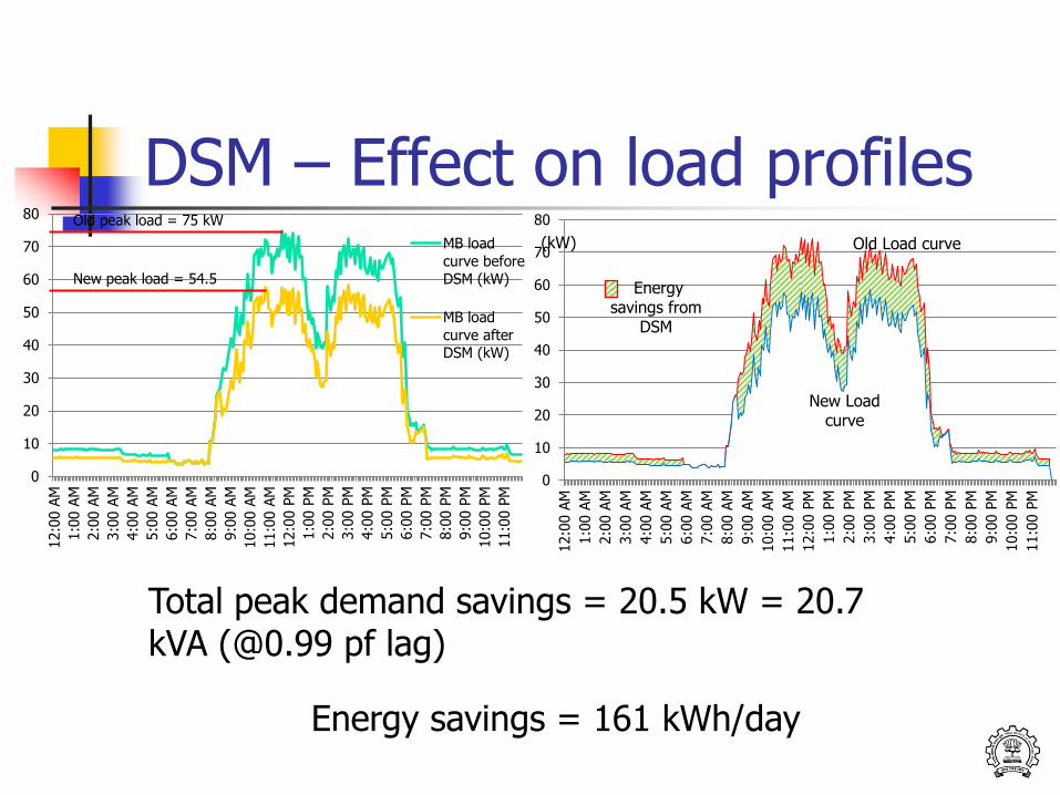
DSM – Effect on load profiles

0

10

20

30

40

50

60

70

80

12:0

0 A

M

1:0

0 A

M

2:0

0 A

M

3:0

0 A

M

4:0

0 A

M

5:0

0 A

M

6:0

0 A

M

7:0

0 A

M

8:0

0 A

M

9:0

0 A

M

10:0

0 A

M

11:0

0 A

M

12:0

0 P

M

1:0

0 P

M

2:0

0 P

M

3:0

0 P

M

4:0

0 P

M

5:0

0 P

M

6:0

0 P

M

7:0

0 P

M

8:0

0 P

M

9:0

0 P

M

10:0

0 P

M

11:0

0 P

M

MB load

curve beforeDSM (kW)

MB load

curve afterDSM (kW)

Old peak load = 75 kW

New peak load = 54.5

0

10

20

30

40

50

60

70

80

12:0

0 A

M

1:0

0 A

M

2:0

0 A

M

3:0

0 A

M

4:0

0 A

M

5:0

0 A

M

6:0

0 A

M

7:0

0 A

M

8:0

0 A

M

9:0

0 A

M

10:0

0 A

M

11:0

0 A

M

12:0

0 P

M

1:0

0 P

M

2:0

0 P

M

3:0

0 P

M

4:0

0 P

M

5:0

0 P

M

6:0

0 P

M

7:0

0 P

M

8:0

0 P

M

9:0

0 P

M

10:0

0 P

M

11:0

0 P

M

Energy savings from

DSM

New Load curve

Old Load curve (kW)

Total peak demand savings = 20.5 kW = 20.7 kVA (@0.99 pf lag)

Energy savings = 161 kWh/day

Load Management Steps

Analysis of Load variations

Identification of Controllable Loads

Selection of Control Option

Implementation strategy

Common LM Options (SEB)

Staggering of working hours of large consumers

Staggering of holidays of large consumers

Specified energy and power quotas for major consumers

Rostering of agricultural loads

Curtailment of demand - service interruptions (load shedding)

Load Management Options

Direct Load Control (DLC) – Utility has control of directly switching off customer loads

Interruptible Load Control (ILC)- Utility provides advance notice to customers to switch off loads

Time of Use (TOU) Tariffs – price signal provided – customer decides response

DLC Control Strategies

Cycling - Groups of loads switched off for short time periods to reduce system diversified demand

Payback control- Groups of devices switched off for periods upto 6 hours

Cycling preferable as payback control imposes larger than normal load when switched on

LM Options

Cool Storage – Chilled water , Ice storage- operate compressor during off-peak

Water pumping systems

Cogeneration – Operating strategy

Evaluate Process Storage possibilities

Power pooling

DLC- India

Central Air Conditioning- cities like Delhi, Mumbai … VHF controlled or timer controlled - cycling

Agricultural pumping Reconfiguration of Distribution system

Individual controllers on pumps

Timer Control

Municipal Water Pumping

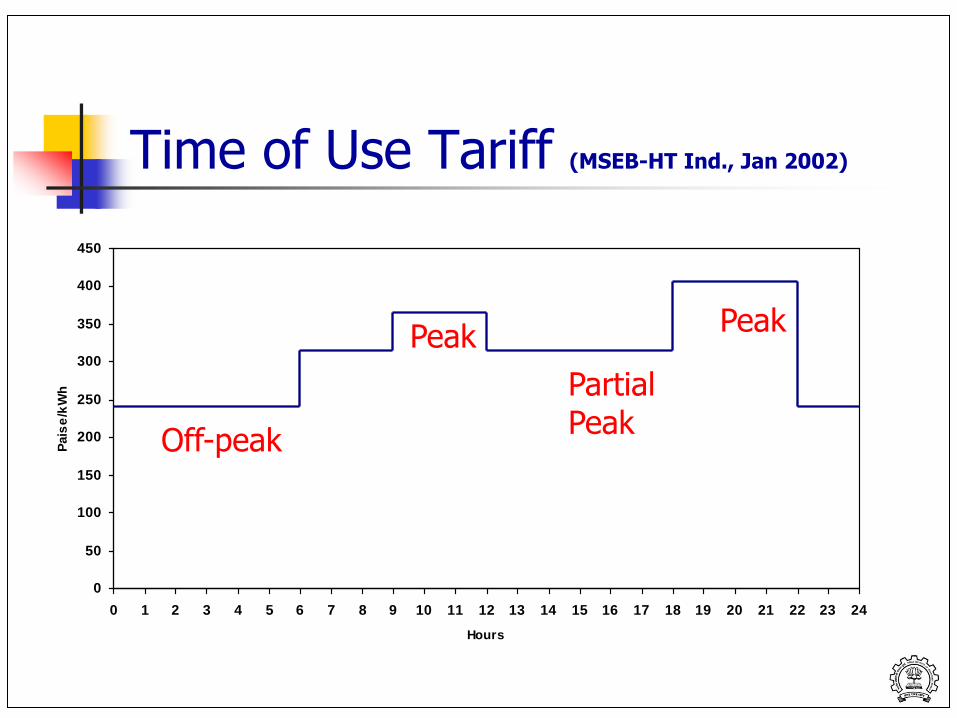
Time of Use Tariff (MSEB-HT Ind., Jan 2002)

0

50

100

150

200

250

300

350

400

450

0 1 2 3 4 5 6 7 8 9 10 11 12 13 14 15 16 17 18 19 20 21 22 23 24

Hours

Pais

e/k

Wh

Off-peak

Peak

Partial Peak

Peak

39

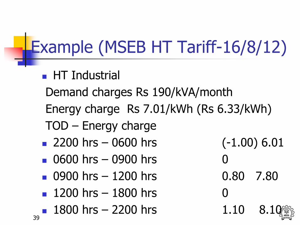
Example (MSEB HT Tariff-16/8/12)

HT Industrial

Demand charges Rs 190/kVA/month

Energy charge Rs 7.01/kWh (Rs 6.33/kWh)

TOD – Energy charge

2200 hrs – 0600 hrs (-1.00) 6.01

0600 hrs – 0900 hrs 0

0900 hrs – 1200 hrs 0.80 7.80

1200 hrs – 1800 hrs 0

1800 hrs – 2200 hrs 1.10 8.10

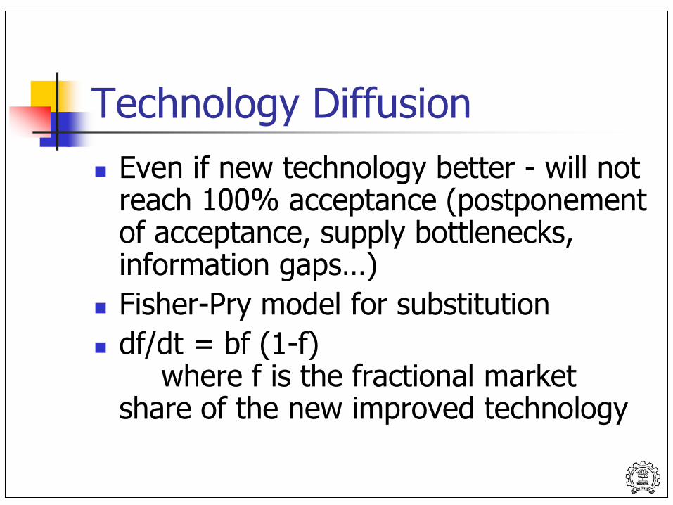
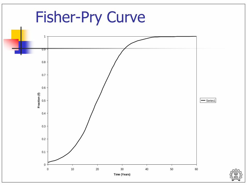
Technology Diffusion

Even if new technology better - will not reach 100% acceptance (postponement of acceptance, supply bottlenecks, information gaps…)

Fisher-Pry model for substitution

df/dt = bf (1-f) where f is the fractional market share of the new improved technology

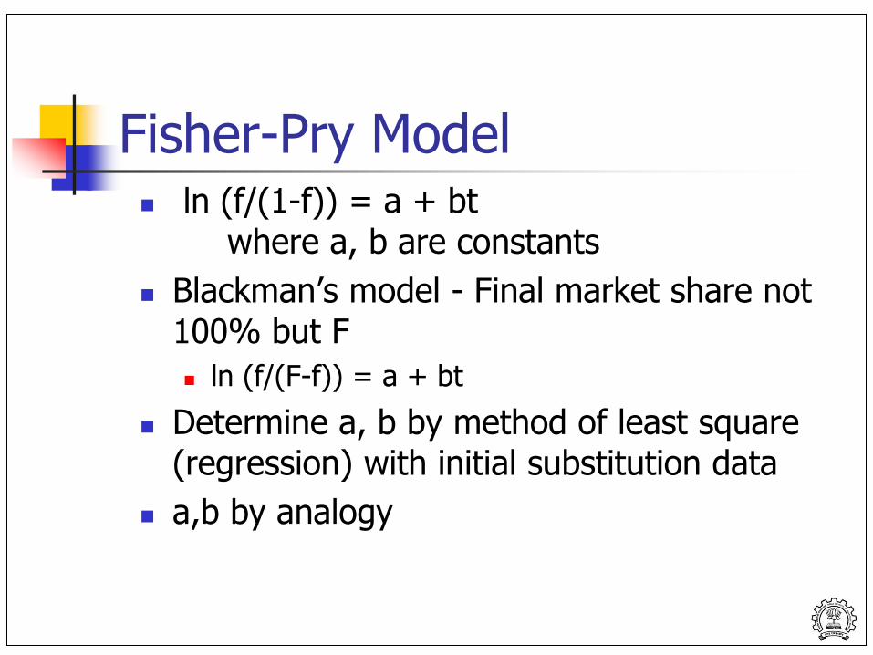
Fisher-Pry Model ln (f/(1-f)) = a + bt

where a, b are constants

Blackman’s model - Final market share not 100% but F

ln (f/(F-f)) = a + bt

Determine a, b by method of least square (regression) with initial substitution data

a,b by analogy

0

0.1

0.2

0.3

0.4

0.5

0.6

0.7

0.8

0.9

1

0 10 20 30 40 50 60

Time (Years)

Fra

cti

on

(f)

Series1

Fisher-Pry Curve

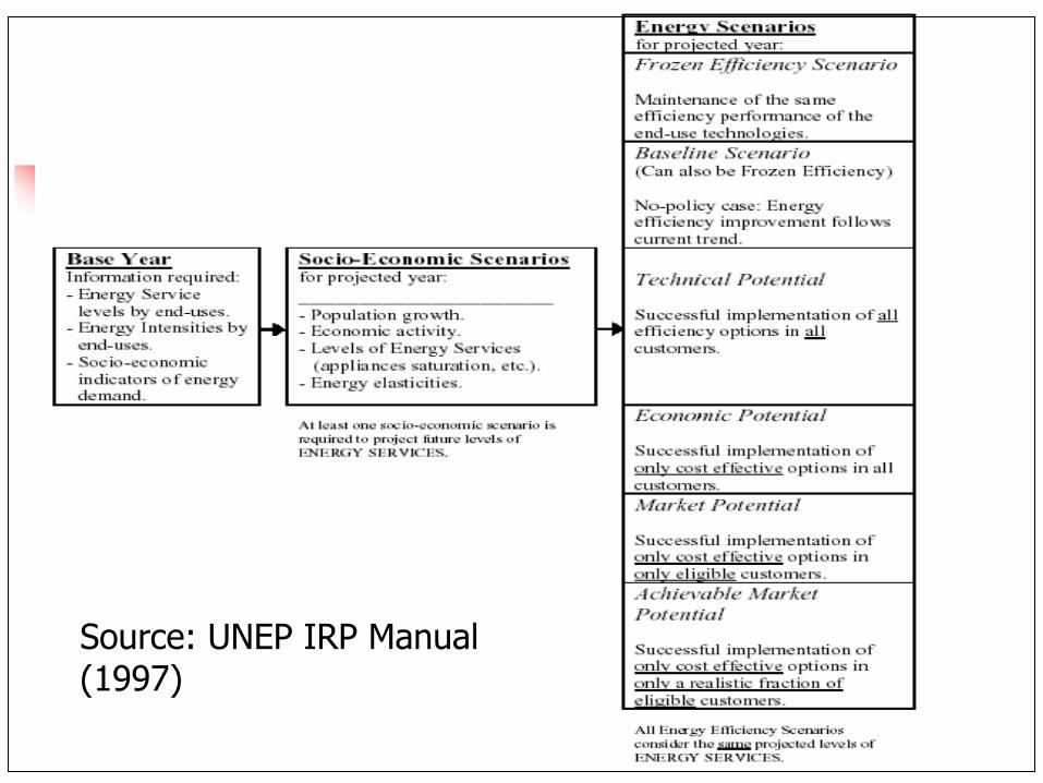
Source: UNEP IRP Manual (1997)

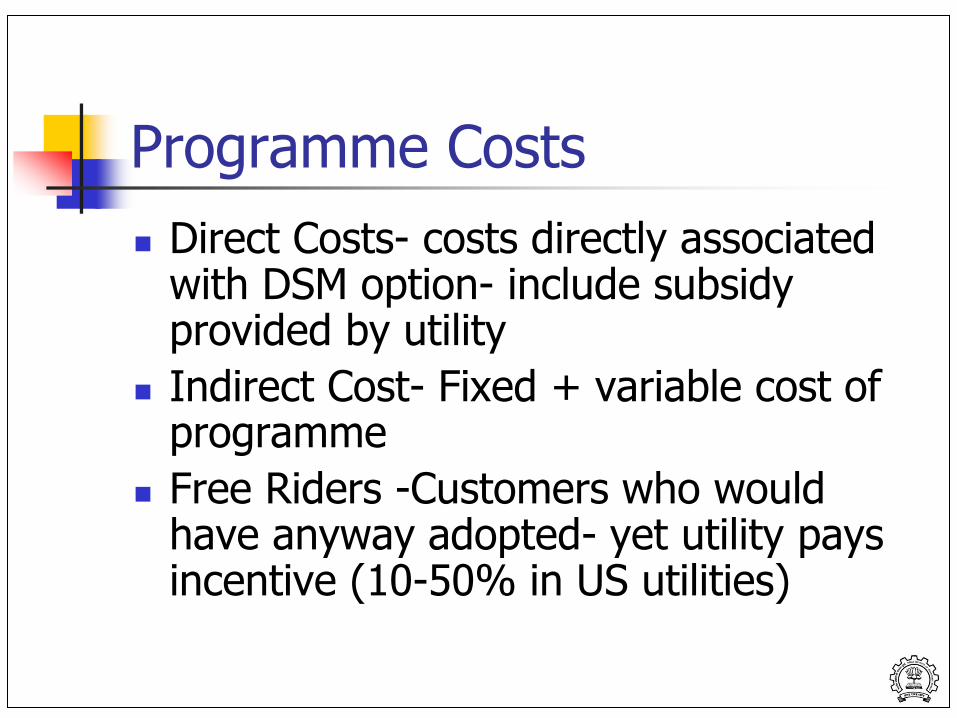
Programme Costs

Direct Costs- costs directly associated with DSM option- include subsidy provided by utility

Indirect Cost- Fixed + variable cost of programme

Free Riders -Customers who would have anyway adopted- yet utility pays incentive (10-50% in US utilities)

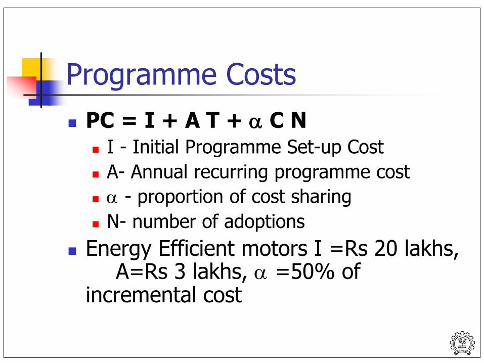
Programme Costs

PC = I + A T + C N I - Initial Programme Set-up Cost

A- Annual recurring programme cost

- proportion of cost sharing

N- number of adoptions

Energy Efficient motors I =Rs 20 lakhs, A=Rs 3 lakhs, =50% of incremental cost

DSM Evaluation

Pre & Post programme metering

Analysis of Customer Billing data

Engineering analysis- physical based models

Questionnaires & Survey

Statistical Modelling- demographics, economics

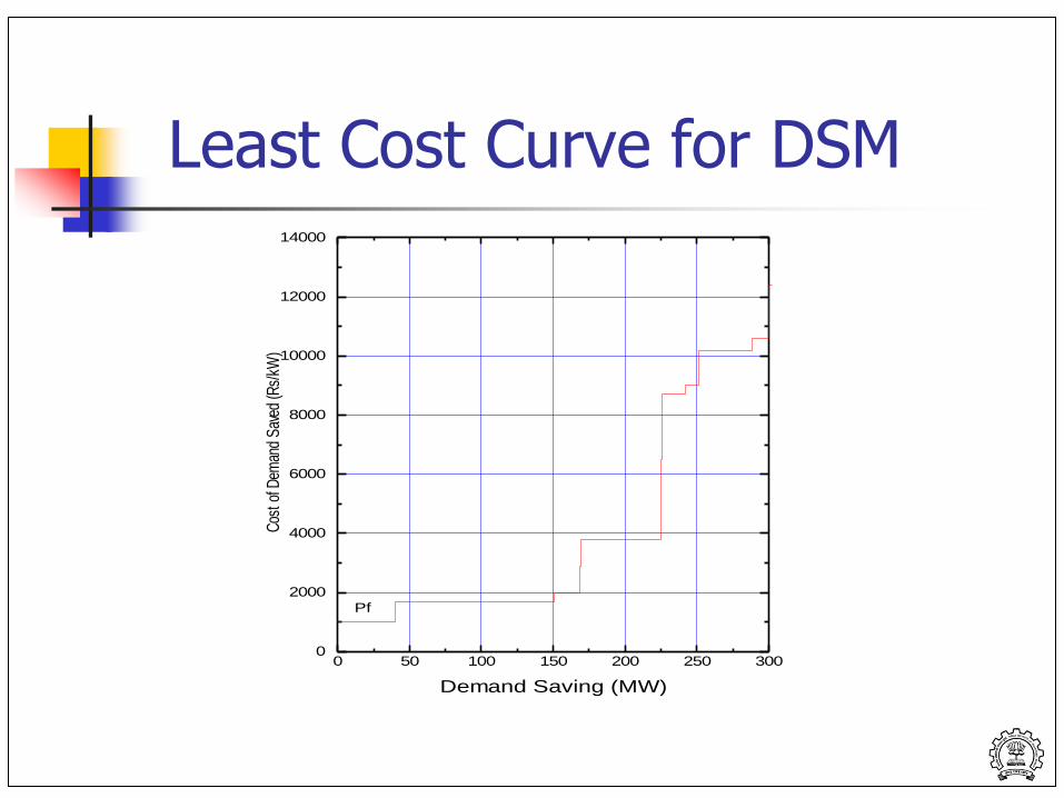
0 50 100 150 200 250 3000

2000

4000

6000

8000

10000

12000

14000

Pf

Cos

t of D

eman

d S

aved

(Rs/

kW)

Demand Saving (MW)

Least Cost Curve for DSM

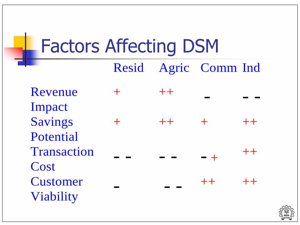
Factors Affecting DSM Resid Agric Comm Ind

Revenue

Impact

+ ++ - - -

Savings

Potential

+ ++ + ++

Transaction

Cost- - - - - +

++

Customer

Viability- - - ++ ++

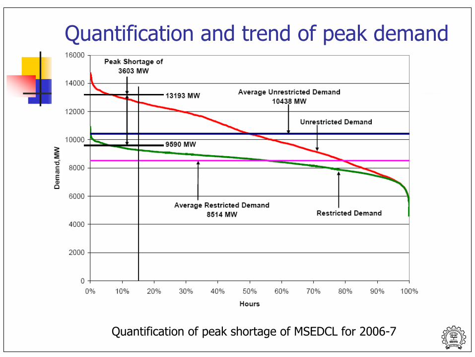
Quantification and trend of peak demand

Quantification of peak shortage of MSEDCL for 2006-7

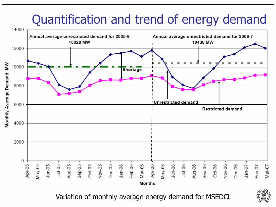
Variation of monthly average energy demand for MSEDCL

Quantification and trend of energy demand

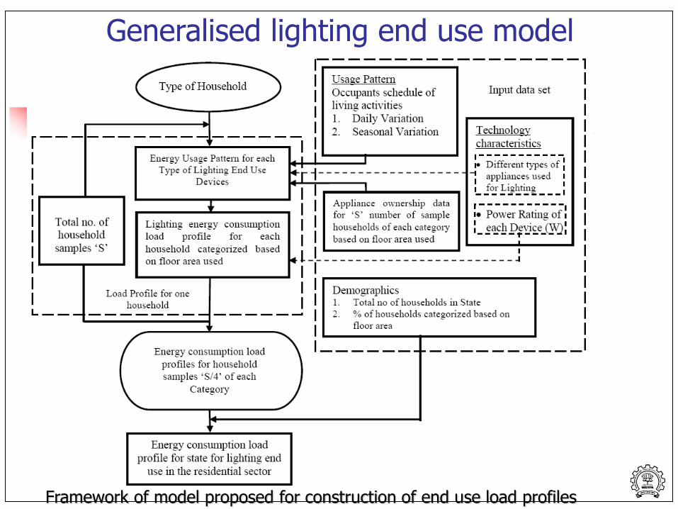
Generalised lighting end use model

Framework of model proposed for construction of end use load profiles

Economic analysis from different perspectives

Economic analysis from perspective of Utilities

0

0.5

1

1.5

2

2.5

3

0 500 1000 1500 2000 2500 3000 3500 4000

Energy Saved/ Purchased in GWh

Co

st

of

Sa

ve

d E

ne

rgy

in

Rs

/kW

h

0

0.5

1

1.5

2

2.5

3

Av

era

ge

En

erg

y P

urc

ha

se

Co

st

in R

s/k

Wh

Energy Purchased by MSEDCL

Energy Saved by Lighting Energy Efficiency

Highest Power generation cost of MSPGCL = 1.81 Rs/kWh

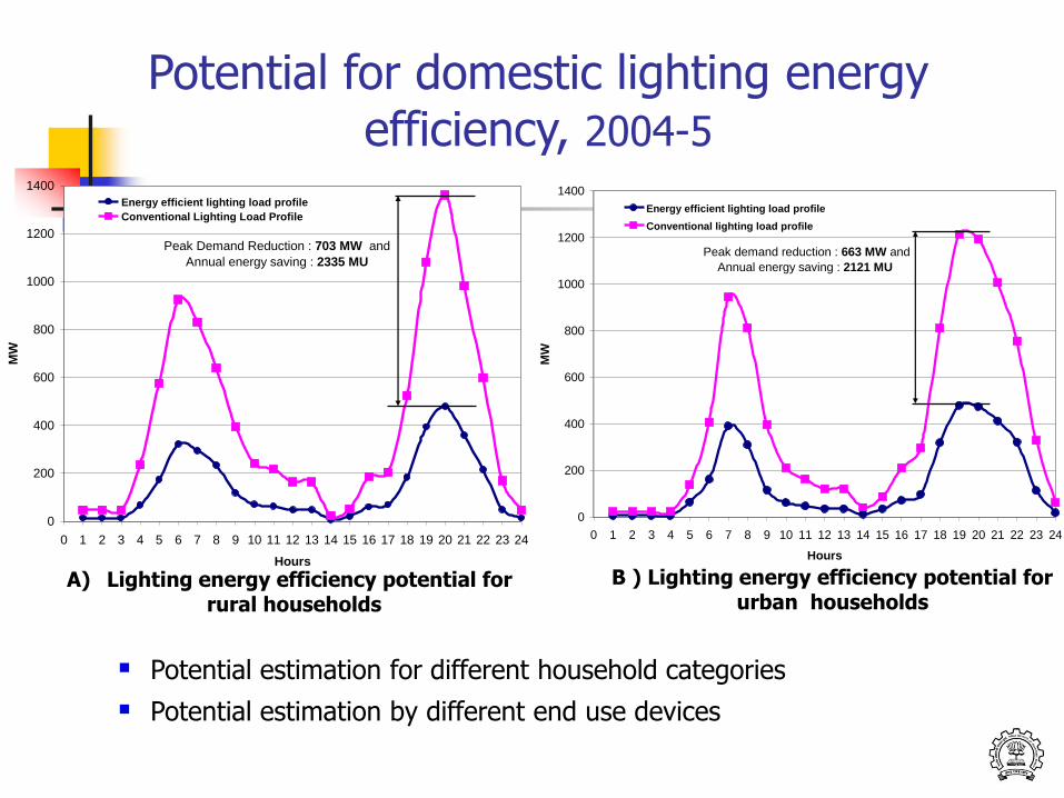
Potential for domestic lighting energy efficiency, 2004-5

Potential estimation for different household categories

Potential estimation by different end use devices

0

200

400

600

800

1000

1200

1400

0 1 2 3 4 5 6 7 8 9 10 11 12 13 14 15 16 17 18 19 20 21 22 23 24

Hours

MW

Energy efficient lighting load profile

Conventional Lighting Load Profile

Peak Demand Reduction : 703 MW and

Annual energy saving : 2335 MU

0

200

400

600

800

1000

1200

1400

0 1 2 3 4 5 6 7 8 9 10 11 12 13 14 15 16 17 18 19 20 21 22 23 24

HoursM

W

Energy efficient lighting load profile

Conventional lighting load profile

Peak demand reduction : 663 MW and

Annual energy saving : 2121 MU

A) Lighting energy efficiency potential for rural households

B ) Lighting energy efficiency potential for urban households

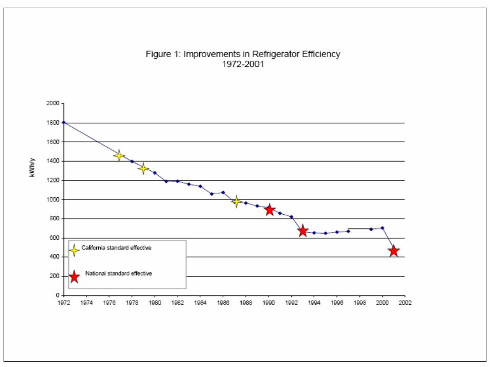
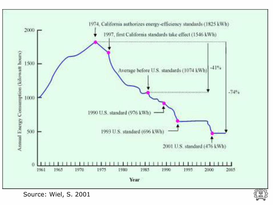
Source: Wiel, S. 2001

S. No.

Equipment

Rating

Initial cost

(Rs)

Annual

Electricity

Cost (Rs)

ALCC (Rs)

Cost of electricity

as %

of ALCC

1

Motor

20 hp

45,000

600,000

605,720

99.0

2

EE Motor

20 hp

60,000

502,600

512,700

98.0

3

Incandescent

Lamp

100 W

10

1168

1198

97.5

4

CFL

11 W

350

128

240

53.6

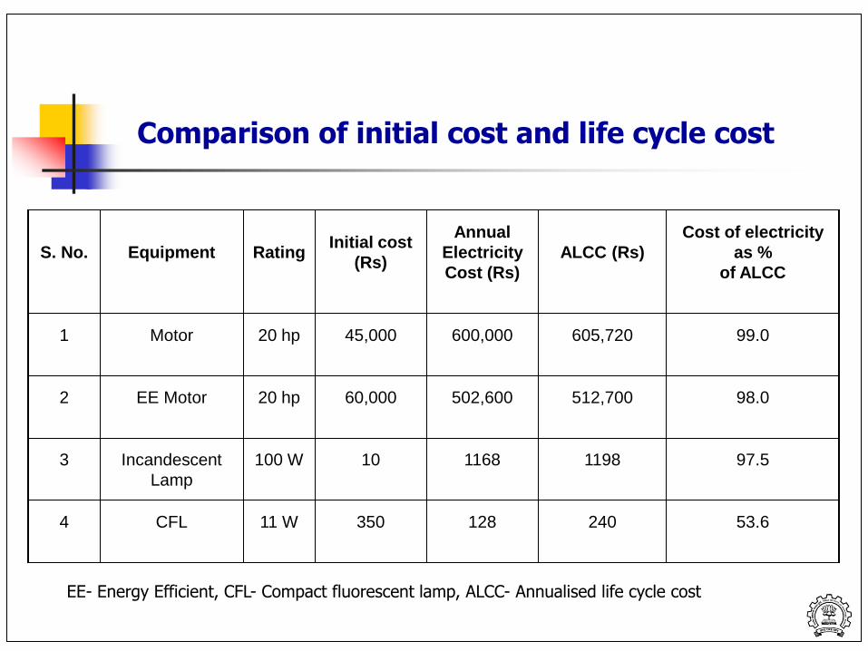
Comparison of initial cost and life cycle cost

EE- Energy Efficient, CFL- Compact fluorescent lamp, ALCC- Annualised life cycle cost

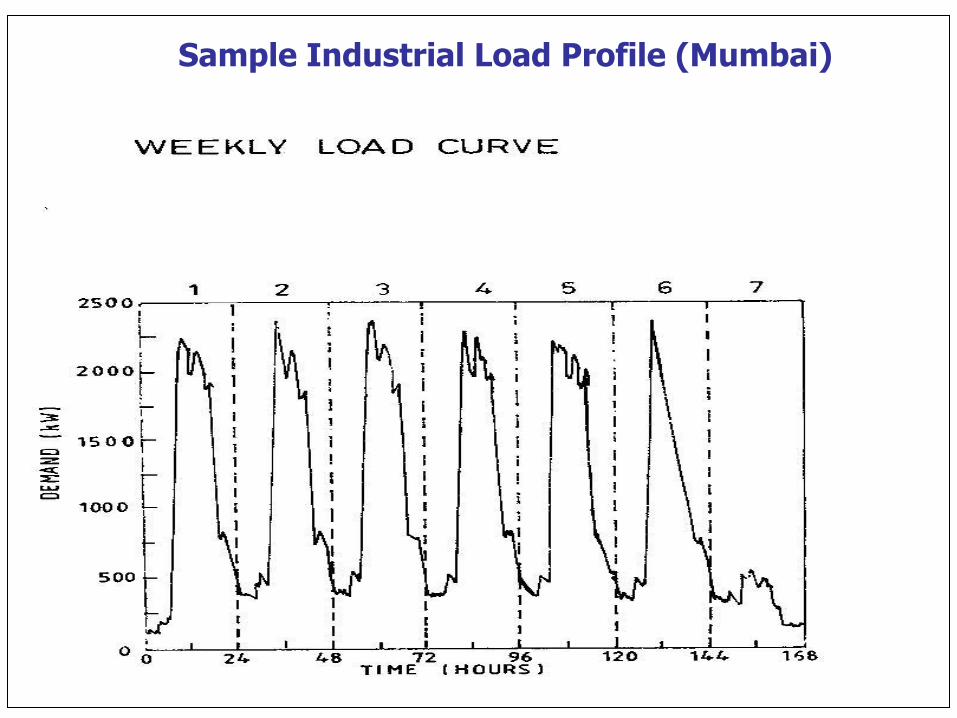
Sample Industrial Load Profile (Mumbai)

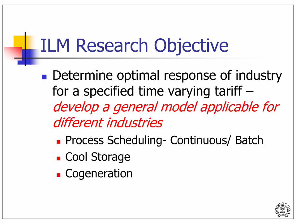
ILM Research Objective

Determine optimal response of industry for a specified time varying tariff –develop a general model applicable for different industries

Process Scheduling- Continuous/ Batch

Cool Storage

Cogeneration

Process Scheduling

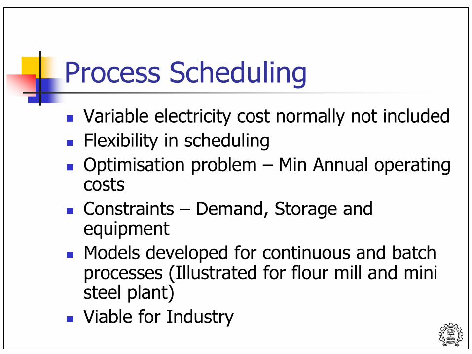
Variable electricity cost normally not included

Flexibility in scheduling

Optimisation problem – Min Annual operating costs

Constraints – Demand, Storage and equipment

Models developed for continuous and batch processes (Illustrated for flour mill and mini steel plant)

Viable for Industry

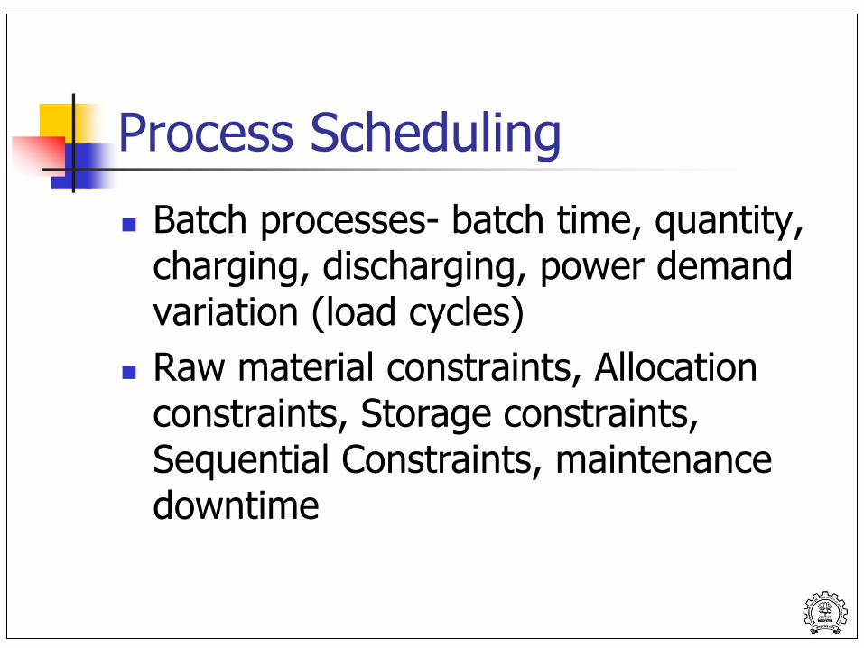
Process Scheduling

Batch processes- batch time, quantity, charging, discharging, power demand variation (load cycles)

Raw material constraints, Allocation constraints, Storage constraints, Sequential Constraints, maintenance downtime

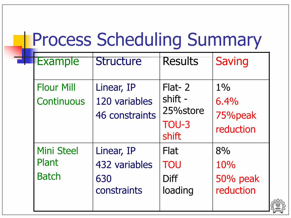
Process Scheduling Summary Example Structure Results Saving

Flour Mill

Continuous

Linear, IP

120 variables

46 constraints

Flat- 2 shift - 25%store

TOU-3 shift

1%

6.4%

75%peak

reduction

Mini Steel Plant

Batch

Linear, IP

432 variables

630 constraints

Flat

TOU

Diff loading

8%

10%

50% peak reduction

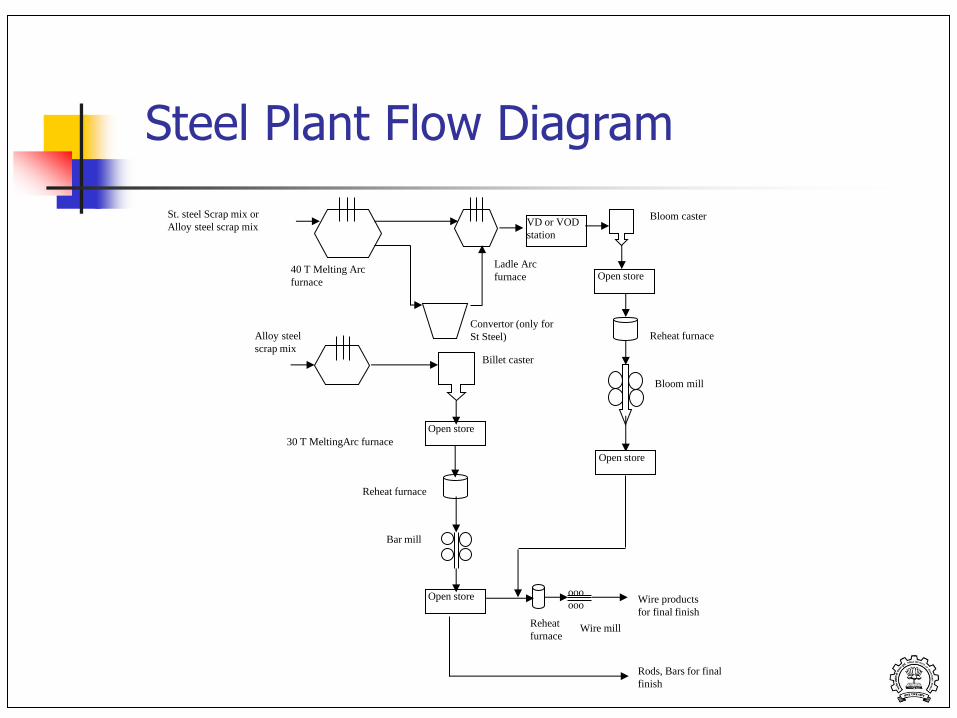
30 T MeltingArc furnace

Bar mill

Wire mill

40 T Melting Arc

furnace

St. steel Scrap mix or

Alloy steel scrap mix

Alloy steel

scrap mix

Convertor (only for

St Steel)

Ladle Arc

furnace

VD or VOD

station

Bloom caster

Billet caster

Bloom mill

ooo

ooo

Reheat furnace

Reheat furnace

Reheat

furnace

Wire products

for final finish

Rods, Bars for final

finish

Open store

Open store

Open store

Open store

Steel Plant Flow Diagram

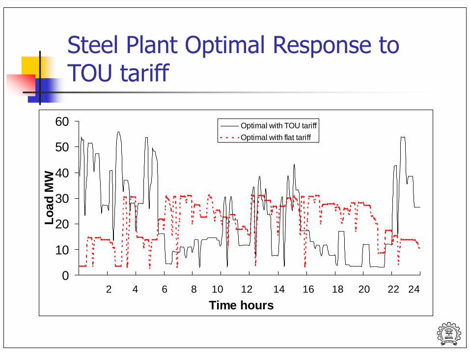
0

10

20

30

40

50

60

Time hours

Lo

ad

MW

Optimal with TOU tariff

Optimal with flat tariff

2 4 6 8 10 12 14 16 18 20 22 24

Steel Plant Optimal Response to TOU tariff

Cool Storage

Cool Storage – Chilled water operate compressor during off-peak

Commercial case study (BSES MDC), Industrial case study (German Remedies)

Part load characteristics compressor,pumps

Non- linear problem – 96 variables, Quasi Newton Method

MD reduces from 208 kVA to 129 kVA, 10% reduction in peak co-incident demand, 6% bill saving

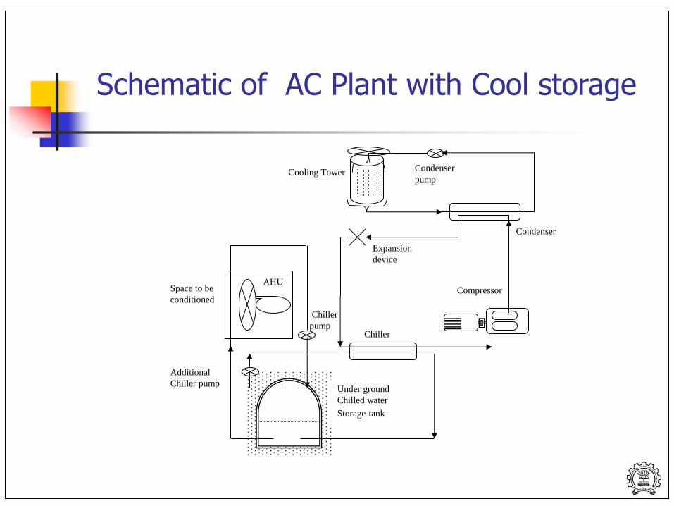
Chiller

pump

AHU

Chiller

Condenser

Compressor

Expansion

device

Condenser

pump Cooling Tower

Additional

Chiller pump Under ground

Chilled water

Storage tank

Space to be

conditioned

Schematic of AC Plant with Cool storage

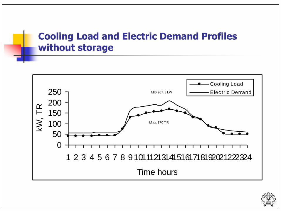
Cooling Load and Electric Demand Profiles without storage

M ax.170 T R

M D 207.8 kW

0

50

100

150

200

250

1 2 3 4 5 6 7 8 9101112131415161718192021222324

Time hours

kW

, T

R

Cooling Load

Elec tric Demand

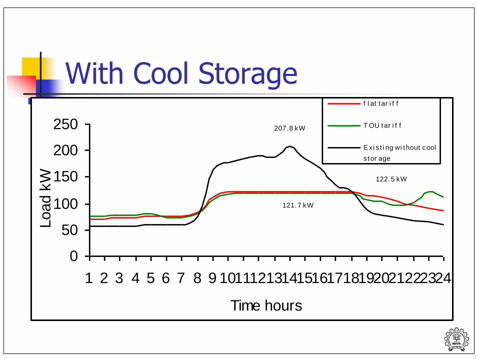
With Cool Storage

121.7 kW

122.5 kW

207.8 kW

0

50

100

150

200

250

1 2 3 4 5 6 7 8 9 101112131415161718192021222324

Time hours

Load k

W

f l at tar i f f

T OU tar i f f

Exi st i ng wi thout cool

stor age

Cogeneration

Process Steam, Electricity load vary with time

Optimal Strategy depends on grid interconnection(parallel- only buying, buying/selling) and electricity,fuel prices

For given equipment configuration, optimal operating strategy can be determined

GT/ST/Diesel Engine – Part load characteristics – Non Linear

Illustrative example for petrochemical plant- shows variation in flat/TOU optimal.

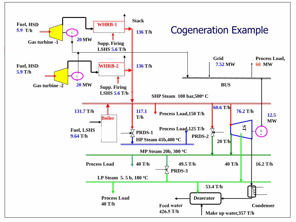
LP Steam 5. 5 b, 180 oC

Gas turbine -1

Boiler

ST

PRDS-1

PRDS-3

Condenser

Deaerator

Process Load

Process Load

40 T/h

G

1

G

4

Process Load,

60 MW

BUS

Grid

7.52 MW

SHP Steam 100 bar,500o C

HP Steam 41b,400 oC

Fuel, LSHS

9.64 T/h

WHRB-1

Supp. Firing

LSHS 5.6 T/h

Stack

20 MW

Process Load,125 T/h

Process Load,150 T/h

MP Steam 20b, 300 oC

PRDS-2

Gas turbine -2

G

1

WHRB-2

Supp. Firing

LSHS 5.6 T/h

20 MW

Fuel, HSD

5.9 T/h

136 T/h

136 T/h

131.7 T/h 12.5

MW

76.2 T/h 60.6 T/h

117.1

T/h

40 T/h 49.5 T/h 16.2 T/h

20 T/h

40 T/h

53.4 T/h

Make up water,357 T/h

Cogeneration Example

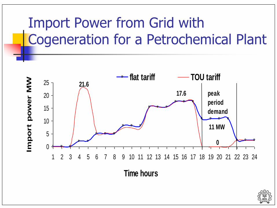
Import Power from Grid with Cogeneration for a Petrochemical Plant

11 MW

17.6

21.6

00

5

10

15

20

25

1 2 3 4 5 6 7 8 9 10 11 12 13 14 15 16 17 18 19 20 21 22 23 24

Time hours

Imp

ort p

ow

er M

W

flat tariff TOU tariff

peak

period

demand

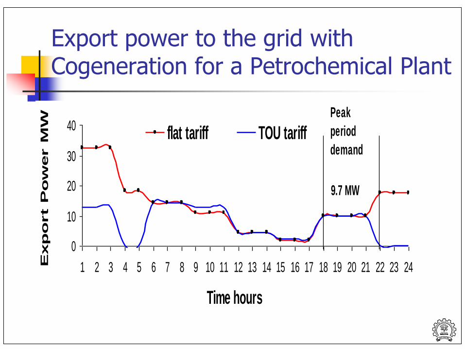
Export power to the grid with Cogeneration for a Petrochemical Plant

0

10

20

30

40

1 2 3 4 5 6 7 8 9 10 11 12 13 14 15 16 17 18 19 20 21 22 23 24

Time hours

Exp

ort P

ow

er M

W

flat tariff TOU tariff

9.7 MW

Peak

period

demand

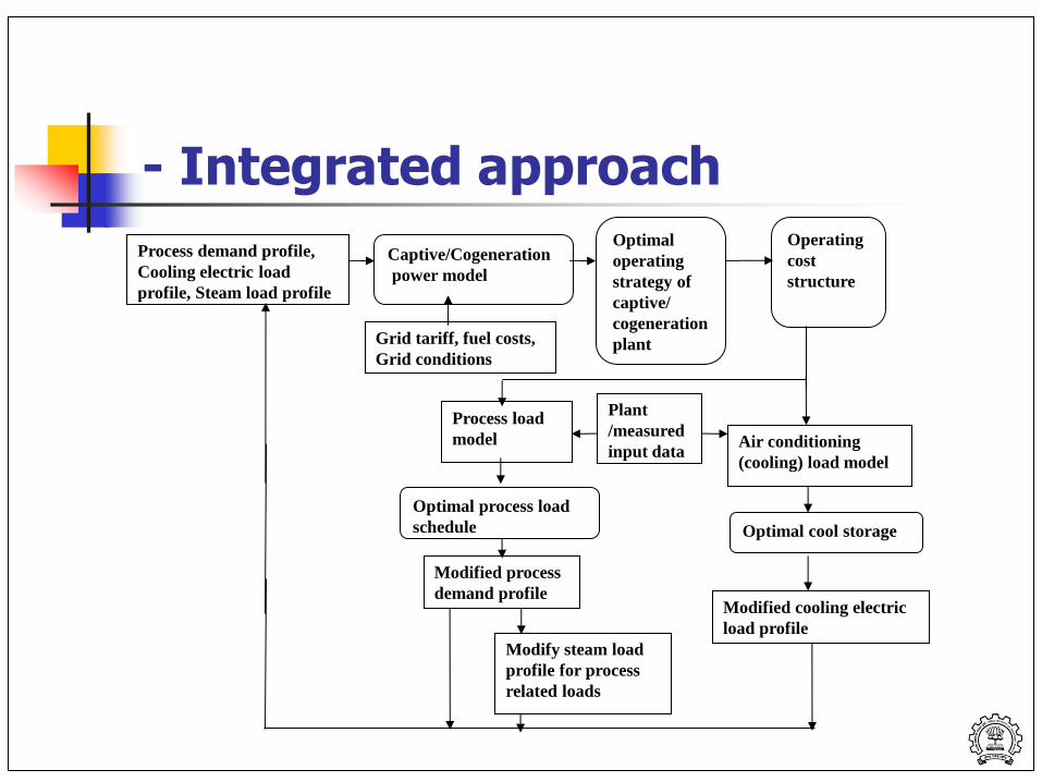
- Integrated approach Operating

cost

structure

Optimal

operating

strategy of

captive/

cogeneration

plant

Captive/Cogeneration

power model

Grid tariff, fuel costs,

Grid conditions

Modified process

demand profile

Process demand profile,

Cooling electric load

profile, Steam load profile

Process load

model

Air conditioning

(cooling) load model

Optimal process load

schedule

Optimal cool storage

Plant

/measured

input data

Modified cooling electric

load profile

Modify steam load

profile for process

related loads

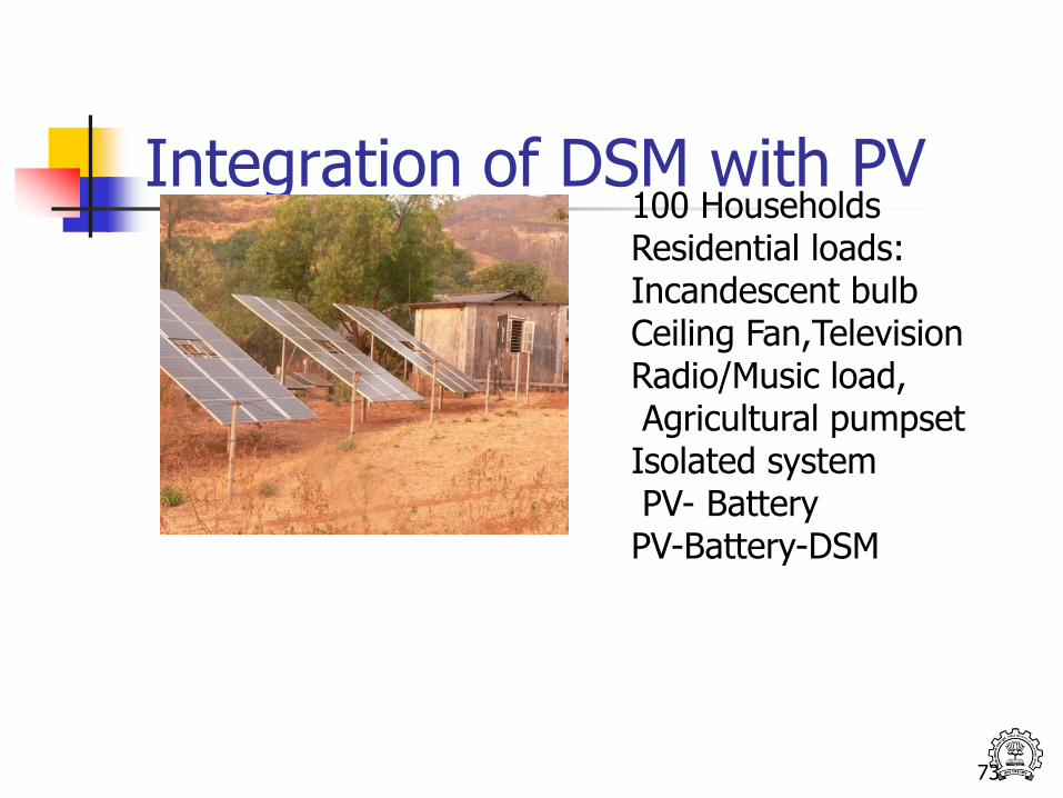
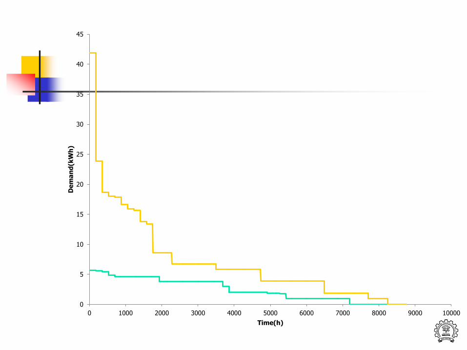
Integration of DSM with PV

73

100 Households Residential loads: Incandescent bulb Ceiling Fan,Television Radio/Music load, Agricultural pumpset Isolated system PV- Battery PV-Battery-DSM

0

2

4

6

8

10

12

14

16

18

20

0 4 8 12 16 20 24

La

od

of

are

a(k

W)

Time of day(h)

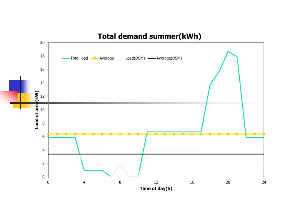
Total demand summer(kWh)

Total load Average Load(DSM) Average(DSM)

0

5

10

15

20

25

30

35

40

45

0 1000 2000 3000 4000 5000 6000 7000 8000 9000 10000

De

ma

nd

(kW

h)

Time(h)

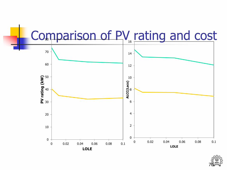
Comparison of PV rating and cost

76

0

10

20

30

40

50

60

70

80

0 0.02 0.04 0.06 0.08 0.1

PV

ra

tin

g (

kW

)

LOLE

0

2

4

6

8

10

12

14

16

0 0.02 0.04 0.06 0.08 0.1

ALC

C(L

acs)

LOLE

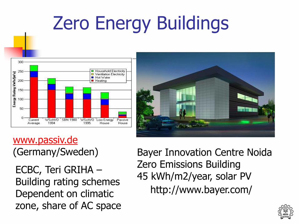
Zero Energy Buildings

www.passiv.de (Germany/Sweden)

http://www.bayer.com/

Bayer Innovation Centre Noida Zero Emissions Building 45 kWh/m2/year, solar PV

ECBC, Teri GRIHA – Building rating schemes Dependent on climatic zone, share of AC space

MULTIPLE FACETS OF CONSTRUCTING A GREEN BUILDING

SOLAR DECATHLON - RESEARCH AREAS

Structural Analysis

Materials

Prefab construction

Passive Architecture & Simulation

Solar Potential & PV

HVAC Design

MEP System Design

Instrumentation & Control Systems

COLLABORATION Inter-disciplinary research – Team has students from 13 different disciplines Diverse team consisting of students from all major programmes – PhD, M.Tech, Undergraduate (2nd, 3rd, 4th, 5th Years) Collaboration and interfacing with industry experts

Efficiency and DSM

Rebound Effect

Transaction Costs

Level Playing Field

Needed a Paradigm Change – Focus on Energy Services

Shortage of Supply to Longage of Demand

80

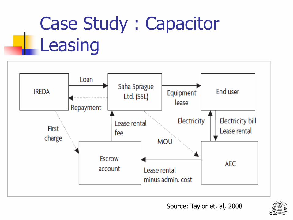
Case Study : Capacitor Leasing

81 Source: Taylor et, al, 2008

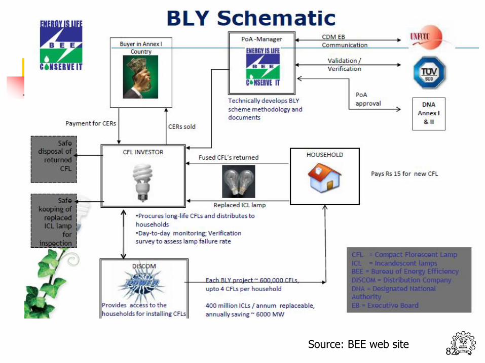
82 Source: BEE web site

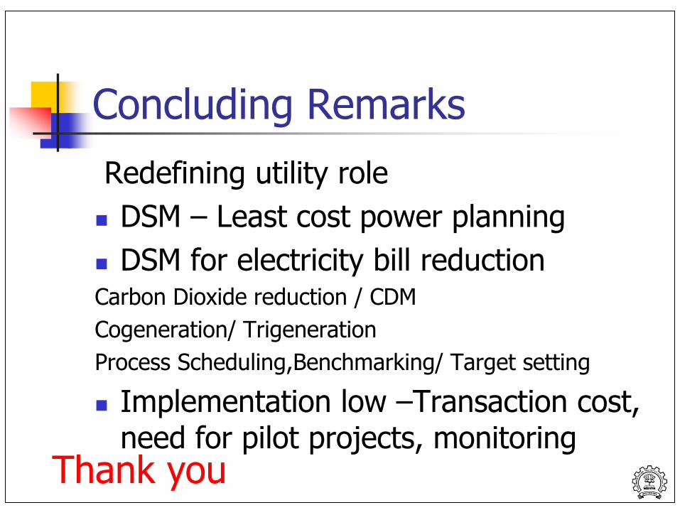
Concluding Remarks

Redefining utility role

DSM – Least cost power planning

DSM for electricity bill reduction Carbon Dioxide reduction / CDM

Cogeneration/ Trigeneration

Process Scheduling,Benchmarking/ Target setting

Implementation low –Transaction cost, need for pilot projects, monitoring

Thank you

References

J.K. Parikh , B.S.Reddy and R.Banerjee, Planning for Demand Side Management in the Electricity sector, Tata McGraw Hill , New Delhi,1994.

S Ashok and Rangan Banerjee, Optimal Operation of Industrial Cogeneration for Load Management, IEEE Transactions on Power Systems, Vol 18, No. 2, May 2003.

S. Ashok and Rangan Banerjee, Optimal cool storage capacity for load management, Energy 28 (2003) 115-126.

R.Banerjee, "Load management in the Indian power sector using US experience", Energy, Vol 23, 1998 , pp 961-973

J. K. Parikh, B. S. Reddy, R. Banerjee & S. Koundinya," DSM survey in India: awareness, barriers and implementability", Energy, Vol 21, No 10, pp 955 - 966, 1996.

P.Du Pont et al, Lessons learnt from implementation of DSM in Thailand, Energy Policy,1998

Vishal S., U.N. Gaitonde and R. Banerjee, ‘Model based energy benchmarking for glass furnace’, Energy Conversion and Management, 2718-2738, 2007.

C.J. More, S. Saikia and R. Banerjee ,An Analysis of Maharashtra's Power Situation’, in Economic and Political Weekly, 2007.