Demand Uncertainty and Price Maintenance:Markdowns as Destructive Competition

Raymond Deneckere†, Howard P. Marvel‡ and James Peck‡

August 1995

† University of Wisconsin-Madison‡ The Ohio State University

We would like to express our special thanks R. Preston McAfee for many helpful suggestions.We are also grateful to participants in the 1994 Northwestern University Workshop in Indus-trial Organization, as well as seminars at Pennsylvania State University, the U.S. Federal TradeCommission, and the Canadian Bureau of Competition Policy for their comments. Peck ac-knowledges financial support from NSF grant SBR-9409882.

1 Introduction

The possibility of “destructive” or “ruinous” competition has long been offered as a poten-

tially important defect of market systems. Early economists and policy makers alike were

concerned that when firms were required to make up-front commitments prior to the res-

olution of demand uncertainty, in the event of slack demand “overproduction” could result

in ruinous competition, impairing the very existence of the industry in question.1 The first

fundamental theorem of welfare economics, however, predisposes modern economists to be

skeptical about arguments that too much competition can be destructive.2 In the case of a

monopolistic manufacturer selling to retailers, intuition might suggest that downstream com-

petition minimizes retail profit margins and allows the manufacturer to manipulate the final

retail price with its wholesale price, thereby extracting all available surplus. Even were down-

stream competition somehow to hurt the manufacturer, it would seem that consumers would

be better off, so that competition could not truly be termed destructive. In this paper, we show

that this intuition can be wrong: manufacturers may be better off by committing to a minimum

resale price for their products sold through independent retailers. This guarantee of a stable

market may induce retailers to order larger inventories than had retail markets been permitted

to clear. The manufacturer may thus prefer to prevent unfettered retail competition, as it is

“destructive” to inventory holdings and to expected sales. Surprisingly, we demonstrate that

permitting manufacturers to set minimum resale prices can Pareto dominate retail market

clearing. Consumers as well as manufacturers may prefer resale price maintenance (RPM) to

retail market clearing, with retailers earning zero expected profits in both cases.

Destructive competition in this paper is not merely another “second-best” phenomenon.

The retail market we model is perfectly competitive, with no externalities or other relevant

1See Hovenkamp (1989) for a history of such concerns. Leading economists such as Frank Taussig and JohnMaurice Clark credited ruinous competition as a serious threat to the market economy, as did influential juristsOliver Wendell Holmes, Jr., and Louis Brandeis. Holmes in particular complained that in a market where informa-tion was imperfect, one needed to be concerned about “transitory cheapness unprofitable to the community as awhole.” See Holmes’ dissent in Dr. Miles Medical Co. v. John D. Park and Sons, Co., 220 U.S. 373 (1911), p. 412.

2One notable exception is the theory of contestable markets (Baumol, Panzar and Willig, 1982), which devel-ops conditions on the cost function under which incumbents are vulnerable to hit-and-run entry, thereby caus-ing competition to be unstable. Our approach does not rely on the indivisibilities that are at the heart of the(non)sustainability literature.

1

market failures. We consider the typical retail situation in which retailers must commit to

inventories prior to the resolution of demand uncertainty. We show that the competitive

scramble to sell inventories at very low prices should demand be low—as opposed to allowing

the inventories to go to waste—can be destructive.3 We also show, however, that when it is used

to prevent deep discounting of unsold merchandise, RPM can, in some cases, be contrary to

consumer interests. We thus can explain why consumer groups are often vociferous opponents

of RPM.4

Our focus on manufacturer attempts to limit destructive competition leads naturally to

consideration of resale price maintenance, for RPM has long been justified as necessary to

limit such competition among distributors. During its long and contentious history, (Over-

street, 1984; Ippolito, 1988, 1991; Marvel 1994) RPM has been the focus of legislative and

court disputes at both the state and federal levels as well as numerous articles in both pro-

fessional journals and the popular press. Allegations of illegal RPM have been a feature of

a very large number of antitrust cases, several of which have reached the Supreme Court.

RPM was declared a per se violation of the Sherman Act by the Supreme Court in its famous

Dr. Miles decision in 1911.5 The Court noted that an agreement among retailers to set their

prices would clearly be illegal, and concluded that if the manufacturer were permitted to con-

trol resale prices, the same result would obtain. There is, however, very little evidence that

dealer cartels exist or that retailers possess the power to coerce their manufacturer-suppliers

(Marvel 1994). Since the applicable section of the Sherman Act (§1) outlawed combinations in

restraint of trade, the Court later recognized an exception to the rule of per se illegality for

a manufacturer who unilaterally refused to deal with price-cutting retailers.6 This exception

was narrowly defined, however, and while in the 1930’s, 42 states passed laws permitting RPM

3In a related paper (Deneckere, Marvel and Peck, 1994) we have have compared RPM to a game in which retailersmust set prices prior to the resolution of demand uncertainty. In that model, as in the one presented below, RPMis preferred by manufacturers as it supports higher inventories and higher quantities.

4An upstream imperfection in the form of a monopoly manufacturer pricing above marginal cost in order toextract consumer surplus lies at the heart of our theory. Given, however, the large number of products whoseproduction entails high fixed costs, some exercise of market power by manufacturers is unavoidable. Everyexample of the use of RPM of which we are aware involves a branded or unique product that can be expected toface downward-sloping demand.

5Dr. Miles Medical Co. v. John D. Park and Sons, Co., 220 U.S. 373 (1911).6U.S. v. Colgate & Co., 250 U.S. 300 (1919).

2

for intrastate commerce, the practice remained illegal for most retail trade until 1937, when

the Miller-Tydings Act7 amended the Sherman Act to permit RPM contracts for interstate com-

merce where permitted by state law. RPM remained illegal in Texas, Missouri, Vermont, and

the District of Columbia, while its status in the remaining states was generally legal, though

sometimes constrained in ways too complicated to recount here. Over the next forty years, a

number of state courts invalidated RPM statutes as unconstitutional, several states repealed

their laws, and eventually, in 1975, Congress repealed the Miller-Tydings Act, making RPM

again per se illegal.8 In the 1980’s, however, the Supreme Court provided an expansive treat-

ment of its Colgate doctrine permitting unilateral manufacturer imposition of RPM programs,

so that today, RPM has the curious status of being both per se illegal and widely practiced.9

Manufacturers may suggest retail prices, receive dealer complaints, and terminate dealers who

do not adhere to the manufacturer’s desired prices so long as they do not reach agreements

with their remaining dealers to establish prices. Manufacturers may not, however, establish

policies of terminating dealers for setting discounted prices and reinstating those dealers who

stop discounting, for then agreement would be inferred. State Attorney Generals, the Federal

Trade Commission, and the Antitrust Division of the Department of Justice have all indicated

strong hostility to RPM use, pursuing a number of investigations designed to limit the use of

the practice (Marvel 1994).

While it is well understood (Telser, 1960; Marvel and McCafferty, 1984) that manufacturers

may wish to suppress price competition to eliminate free-rider effects and thereby to create

property rights to dealers providing pre-sale promotion,10 our model does not rely on the

existence of such services.11 It is clear that early proponents of fair trade were more concerned

750 Stat. 693, 15 U.S.C.A. §1 (1937).8Consumer Goods Pricing Act of 1975, Public Law 94-145, 89 Stat. 801 (1975).9Business Elecs. Corp. v. Sharp Elecs. Corp., 485 U.S. 717 (1988).

10For example, suppose that a manufacturer invents a new appliance for food preparation, but that the usesof the appliance are not immediately obvious to potential consumers through inspection. It may be essentialthat retailers demonstrate the product’s capabilities. Given that demonstration is a costly service, the retailerproviding demonstrations must charge retail prices sufficient to cover demonstrations as well as the wholesaleprice paid to the manufacturer. Retailers not offering such demonstrations could thereby profit by undercuttingthe prices of demonstrating retail outlets. That is, a customer can visit a costly product demonstration, becomeconvinced to buy the product, and then buy it elsewhere at a lower price. Otherwise identical retailers cannotsurvive if they provide demonstrations. Demonstrations will not, therefore, be provided, an inefficient outcome.

11Ippolito (1991) finds that less than half of litigated RPM cases from 1976-1982 involved complex products forwhich dealer efforts were important to product quality.

3

about “disorderly markets” than about product-specific dealer services. As a judge noted

in an 1874 court opinion, “[t]he prohibition against selling below the trade price is a very

common one between a manufacturer and those who buy of him to sell again, and is intended

to prevent a ruinous competition between sellers of the same article.”12 The American Sugar

Refinery Company, a near-monopoly trust, was a pioneer RPM user (Eichner, 1969; Zerbe,

1969). It marketed sugar through wholesale grocers dependent on such sugar for in excess of

one-third of their business. Pre-sale retail services were not required, nor was the wholesaler

required to attest to the purity of the product, for potential adulterants cost more than the

sugar itself. In this and other contemporary examples, the manufacturer claimed to impose

RPM to counter demand fluctuations that would otherwise destabilize the wholesale market.

The desire to prevent disorderly price fluctuations under market clearing was claimed as the

primary justification for a “fair trade” law enabling RPM by that law’s leading proponent, Louis

Brandeis, who argued that “There must be reasonable restriction upon competition else we

shall see competition destroyed.” (McCraw, p. 102, quoting Brandeis.) Our theory captures

this emphasis on demand uncertainty and inventories without requiring either risk aversion

or bankruptcy costs.13

Subsequent to the 1975 revocation of states’ authority to permit RPM, retail markdowns

have become an increasingly important feature of the U.S. retail distribution landscape. De-

fined by the National Retail Federation as “the dollar reduction from the originally set retail

prices of merchandise. . . ,”14 markdowns grew modestly from 6.3% in 1966 to 8.9% in 1975,

and then accelerated to 12% in 1981 and reached 24.7% in 1991.15 In some instances, mark-

downs have proven fatal. Atari games vanished from store shelves following a period of slack

demand and very substantial price cutting. Nintendo, successor to Atari as market leader in

12Nutter v. Wheeler, 18 F. Cas. 497 (C.C.D. Mass. 1874) (No. 10,334).13Rey and Tirole (1986) consider vertical restraints under demand uncertainty. Their model permits manufac-

turers to employ two-part tariffs for sales to retailers, thereby imposing a fixed fee commitment on retailers. Reyand Tirole show that RPM will only be favored when retailers are very risk averse. Unlike our model, however,output is produced after demand is realized.

14National Retail Federation, Merchandising and Operating Results: Fiscal 1991, Department and Specialty Stores,1992 Edition (New York: Business Services, National Retail Federation, 1992), p. 169.

15National Retail Federation, Merchandising and Operating Results. . . , ibid, various editions. This trend does notreflect changes in gross retail margins, which have hovered around 40% throughout the same time period. Grossmargins for retail departments, stated as a percentage of retail department sales, were 37.4% in 1966, peaked at42.9% in 1981, and had declined to 38.2% in 1991.

4

the electronic games market, has been charged with imposing RPM on its retailers. In sec-

tion 5, we show that the electronic games experience is both incompatible with alternative

explanations of RPM and is consistent with the predictions of our model.

We proceed as follows. First, in section 2, we illustrate our argument with a simple example

of how a manufacturer can benefit by suppressing price competition among its retailers. We

demonstrate that suppression of price competition can benefit not only manufacturers and

society generally, but also consumers, even though such consumers are denied the chance to

purchase goods at low prices in the event of slack demand. In section 3 we demonstrate with

considerable generality that the manufacturer will often prefer to suppress retailer competi-

tion. In section 4 we provide sufficient conditions under which total surplus is higher under

RPM than under flexible retail prices. We also provide conditions under which both profits and

consumer surplus are higher under RPM than under flexible retail prices. When alternatives

to market clearing yield higher total surplus, and in particular when that surplus accrues to

both the manufacturer and consumers, the alternative of unrestrictive price competition can

truly be considered destructive. Section 5 offers some concluding remarks.

2 The Model, and an Example

A risk-neutral monopoly manufacturer sells to a continuum of risk-neutral retailers, repre-

sented by an index t ∈ [0,1]. Retailers, in turn, sell to consumers. We assume throughout

that inventories which are left unsold at the end of the demand period have no scrap value.16

Retailers must order and take title to these inventories prior to the demand period so that un-

sold inventories are, to them, a sunk cost—the manufacturer does not offer to accept returns

16While we specify zero scrap value to simplify the analysis, our results merely require that retailers cannotrecoup the full value of their investments in inventories. Such sunk investment costs can come about becauseinventories are costly to hold over to the next demand period or because the goods spoil or become outmoded.If inventory costs were negligible, our assumption would imply that manufacturers refuse to accept returns ofunsold merchandise for full credit. Returns policies may be prohibitive either because of retailer moral hazardor the costs of administering such systems. (Returns are employed for books and magazines, but the costs ofshipping are so large that for paperbacks, only the covers are returned, illustrating both the costs and potentialmoral hazard problems of such schemes.) Returns policies in the presence of demand uncertainty are analyzedin Marvel and Peck (1994).

5

of unsold merchandise.17 We assume that other marginal costs of distribution are constant

and, without loss of generality, normalize them equal to zero.18 To compare RPM and retail

market-clearing, we are interested in the subgame perfect equilibria of the following games:

The RPM Game The manufacturer must first announce its wholesale price, pw , and the min-

imum retail price at which its product may be resold, p. Next, retailers simultaneously

choose how much inventory to hold, prior to the resolution of demand uncertainty. Once

retailer inventories are in place, demand uncertainty is resolved. If the market clearing

price exceeds p, then market clearing determines the price and all transactions. Other-

wise, the retail price is p and retailers find themselves burdened with excess inventories.

In this case, we assume that consumers distribute themselves across the retailers so that

the fraction of inventory sold is the same for all firms.

The Flexible-Price Game The manufacturer initially announces a wholesale price, pw . Retail-

ers then choose simultaneously how much inventory to hold, prior to the resolution of

demand uncertainty. With inventories in place, demand is realized. The retail price is

determined according to supply and demand.

An Example with Two Demand States and Linear Demand

Before presenting a model with general assumptions on demand and its distribution across

different states of the world (see Section 3), we first provide a simple two-state, linear demand

example illustrating the basic economic forces behind our results. In the example, RPM is

17A prototypical example of the type of market to which our model applies is that for “sell-through” videos,that is, movies that are sold, rather than rented, on video cassettes. Manufacturers of such products try tomaintain minimum resale price through minimum advertised pricing (MAP) practices that deny advertising rebatesto dealers failing to adhere to the manufacturer’s preferred price. The Disney Company is an aggressive user ofMAP for its animated videos such as “Snow White,” “The Fox and the Hound,” and “The Return of Jafar.” Thepractice is also common for recorded music. For such products, the window of novelty in which they sell canbe short and uncertain. In addition, as shown in Theorem 1, the low marginal cost of producing copies makesimposing RPM particularly attractive to the manufacturer. See “MAPS for Hot Vids are Hard to Read; Retail Price-Cutting Battles May Erupt,” Billboard, July 16, 1994, p. 8.

18Suppose retailers face a constant marginal cost of inventories, denoted by c1, as well as a constant marginalcost of providing sales, denoted by c2. Inventory holding costs can simply be absorbed into the manufacturer’scost of producing for inventory, and the cost of providing sales can be accommodated by reinterpreting inversedemand as the willingness to pay above c2. More precisely (using the notation of Section 3), retailer profits,manufacturer profits and consumer surplus in the model with inverse demand P(q,α), production cost C(q) andpositive distribution costs are identical to those in the model with inverse demand P(q,α)− c2, production costC(q)− c1q, and no distribution costs.

6

always beneficial to the manufacturer and can (but need not) improve welfare in comparison

to permitting prices to clear the market. Suppose that demand is given by

D(p,θ) =

1− p, with probability 1/2 (low demand state)

θ(1− p), with probability 1/2 (high demand state)(1)

Without loss of generality, we assume θ > 1. Manufacturing costs are assumed to be zero.

Denote the equilibrium price floor as p∗. The equilibrium strategies along the subgame

perfect equilibrium path of the RPM game are as follows:

pw = 1+ θ4θ

,

p∗ = 12, and (2)

q(t) is any integrable function satisfying qRPM =∫ 1

0q(t)dt = θ

2.

Note that the aggregate inventory holdings, qRPM , are uniquely determined, but that inventory

holdings of an individual retailer, denoted by q(t), are not.19 It follows from (2) that expected

consumer surplus is (1 + θ)/16. Manufacturer profits, denoted ΠRPM, are given by ΠRPM =

(1+ θ)/8.

To see why (2) defines an equilibrium, let us calculate profits of retailer t, denotedπRPM(t),

under the assumption that the retail price, pr , equals the price floor, p, in the high demand

state, so we have qRPM ≥ θ(1− p). In the low demand state, the probability of selling a unit is

equal to (1− p)/qRPM, and in the high demand state it is θ(1− p)/qRPM . Consequently,

πRPM(t) =[p(1− p)(1+ θ)

2qRPM− pw

]q(t). (3)

Since no individual retailer can affect qRPM,20 retailer profits in equation (3) are linear in q(t).19The indeterminacy of the function q(t) is an artifact of the continuum. Suppose instead that there were a

finite number of retailers, where each retailer’s strategy is to choose a level of inventory demand. As in our RPMgame, these inventories are then inelastically supplied to the market at any price at least as high as the price floor.It is straightforward to check that the unique equilibrium of the RPM Game is symmetric and that as the numberof retailers approaches infinity, pw and p∗ approach their values given by (2), and total orders approach θ/2.

20If any retailer were able to affect qRPM, that retailer would reduce its inventory holding in an effort to makethe profit margin positive. A positive profit margin, however, is inconsistent with equilibrium as retailers with

7

Equilibrium then requires that the retail profit margin be zero, implying,

p(1− p)(1+ θ)/2 = pwqRPM. (4)

Since the strategies of expression (2) satisfy retailer t’s zero profit condition, (4), for any choice

of q(t), retailer t has no profitable deviation. Therefore the retailer subgame is in equilibrium.

Since the right side of (4) is manufacturer profits, these profits are maximized subject to (4)

whenever the retail price floor is the monopoly price, p = 1/2. The manufacturer is therefore

optimally choosing p = p∗ = 1/2 and pw = (1+ θ)/4θ, so (2) constitutes an equilibrium.21

To analyze the Flexible-Pricing Game, we must consider two cases. If the wholesale price

is low enough, retailers will order inventories sufficient to force the retail price to zero in the

low demand state (case 1). If the wholesale price is higher, inventories will be lower, which

leads to positive retail prices in both demand states (case 2). Because we have a continuum of

retailers, the equilibrium must have retailers earning zero expected profits.

In case 1, retailers receive revenue only in the high demand state. We have ph = 1−qFL/θ,

where qFL is the quantity of inventory ordered and ph is the retail price that clears the market

in the high demand state. Since retailers only earn a positive margin half the time, their

zero profit condition is ph = 2pw . When choosing pw to induce qFL ≥ 1, the manufacturer

therefore earns profits given by

ΠFL = 12

(1− q

FL

θ

)qFL (case 1). (5)

In case 2, we have pl = (1−qFL) > 0 and ph = 1−qFL/θ. The retailer zero expected profit

condition is therefore given by pw = 1−(1+θ)qFL/(2θ).When choosing pw to induce qFL ≤ 1,

manufacturer profits are

ΠFL =[

1− (1+ θ)qFL

2θ

]qFL (case 2). (6)

infinitesimal inventory holdings would then have an incentive to expand. Formally, the requirement that noindividual retailer be able to affect qRPM is reflected in the integrability requirement on q(t).

21When qRPM < θ(1 − p) holds, equation (3) must be altered, but we still must have zero retail profits. Withzero production costs, the manufacturer always prefers to induce full stocking, as in (2).

8

Since the expression in (6) exceeds the expression in (5) for all qFL ≤ 1, and since the optimum

qFL in case 2 is always strictly less than one, the manufacturer optimizes by inducing the level

of inventory holdings that achieves the maximum profit among expressions (5) and (6).

For our example, when θ > 3, maximal profits are obtained along branch (5), so that the

manufacturer abandons state 1 revenues. The overall equilibrium then involves qFL = θ/2,

pw = 1/4, ph = 1/2, pl = 0, and ΠFL = θ/8. Expected consumer surplus equals 1/4 + θ/16

and welfare equals 1/4+ 3θ/16.

When θ < 3, case 2 is observed. The manufacturer then maximizes by choosing qFL =

θ/(1+θ), yielding pw = 1/2, pl = 1/(1+θ), ph = θ/(1+θ), and ΠFL = θ2(1+ θ). Equilibrium

expected surplus and welfare respectively equalθ

4(1+ θ) and3θ

4(1+ θ) . Finally, for θ = 3, the

manufacturer is indifferent between charging pw = 1/4 (inducing qFL = 3/2) and pw = 1/2

(inducing qFL = 3/4).

Comparing equilibrium profits between the RPM game and the flexible pricing game, we

see that regardless of which case applies, the manufacturer always prefers RPM to market

clearing. Indeed, setting a price floor of 1/2 in the RPM Game shores up the retail price in the

low demand state, so retailer revenues are greater than revenues in the Flexible-Price Game,

holding inventories constant. This is because the lowest retail price in the Flexible-Price Game

is strictly less than the monopoly price. In case 2, the RPM wholesale price remains equal to

the Flexible-Price Game wholesale price of 1/2, and retailers compete by increasing inventory

holdings, yielding the manufacturer higher profits. In case 1, retailer inventories are already

maximal in the Flexible-Price Game, but the manufacturer can extract the extra surplus by

raising the wholesale price. In either case, the manufacturer’s profits increase. In section 3,

we provide general conditions under which manufacturer profits and inventories are strictly

higher under RPM.

From the perspective of consumer surplus and total surplus, the preferred institution de-

pends on which case applies, which in turn depends on the nature of the demand uncertainty.

In case 1, consumer and total surplus are higher under flexible retail prices, since the man-

ufacturer “gives up” on the low demand state and allows the retail price to fall to zero. The

9

manufacturer sets a wholesale price sufficient to induce inventory holdings that maximize

receipts in the high demand state. This results in the same inventories as held under RPM.

However, in the low demand state, the inventories are given away in the Flexible-Pricing Game,

instead of being discarded, as in the RPM Game.

In case 2, consumer and total surplus are higher under RPM. The advantage to consumers

of paying a low market-clearing price when demand is low is outweighed by the disadvantage

of paying a high market-clearing price when demand is high. When demand fluctuations are

not too great and when the low demand state is sufficiently likely (so that case 2 applies),

retail market clearing is destructive in the sense that both consumers and the manufacturer

would prefer RPM. Retailers must be compensated for their propensity to compete the price

down when demand is low, giving rise to higher wholesale prices and lower quantity ordered

than under RPM.

3 A General Demand Specification

In this section, we substantially weaken our assumptions on the demand process and the

manufacturer’s production costs in order to provide a more general theory of destructive

retail competition. Because a price floor of zero is equivalent to unfettered market clearing,

the manufacturer obviously cannot be hurt by the ability to set a minimum retail price for its

product. Theorem 1 provides a necessary and sufficient condition for the manufacturer to

strictly prefer to impose a price floor, that is, to enforce resale price maintenance. Theorem 2

shows that equilibrium inventories are always at least as high under RPM as under market

clearing, and provides sufficient conditions for them to be strictly higher.

Let α ∈ [α¯, α] denote the state of demand. We assume that higher α’s are associated

with higher levels of demand. For any Lebesgue-measurable subset A ∈ [α¯, α], denote the

probability-measure of A as µ(A). We do not place any restrictions on the distribution of α,

represented by the distribution function, F . Thus, discrete, absolutely continuous, and mixed

10

distributions are allowed. The support of F is denoted by

supp F = {x ∈ < : F(x + ε)− F(x − ε) > 0 for every ε > 0}

Without loss of generality, we let α¯= inf supp F and α = sup supp F , and assume α

¯< α.

Let D(p,α) denote the final demand for the manufacturer’s product in state α, and let

P(q,α) denote the corresponding inverse demand. To make the problem interesting, we as-

sume that for each α there exists q such that P(q,α) > 0.22 We assume that these functions

are continuous everywhere, and twice continuously differentiable on the interior of the do-

main where they are strictly positive. The revenue functions, R(q,α) and R(p,α), are defined

by

R(q,α) = qP(q,α) and

R(p,α) = pD(p,α).

The following additional notation will be useful. The choke quantity, or quantity for which

the market-clearing price is zero, denoted as q(α), is defined as

q(α) = sup{q : P(q,α) > 0},

and is assumed to be finite.23

Assumption 1 For every α and for every q ∈ [0, q(α)), we have Pα(q,α) > 0, Pq(q,α) < 0,

2Pq(q,α)+ Pqq(q,α) < 0, and Pqα(q,α) > 0.

Notice that Assumption 1 implies Rqα(q,α) > 0 and that Rqq(q,α) < 0 whenever q < q(α).

Let the manufacturer’s cost function be denoted as C(q), and assume

Assumption 2 C(q) : <+ → <+ is a twice continuously differentiable function with C(0) = 0,22All of our results also hold in the limiting case where P(q,α

¯) = 0 for all q, with trivial modifications to the

proofs.23All of our results go through if q(α) is infinite, provided revenue is maximized at a finite quantity, yielding

finite consumer surplus.

11

C′(q) ≥ 0 and C′′(q) ≥ 0.

Consequently, the profit-maximizing quantity, qc(α), the revenue-maximizing quantity, qm(α),

and the revenue-maximizing price, pm(α), as defined below, are well-defined functions of α:

qc(α) = arg maxq{R(q,α)− C(q)}

qm(α) = arg maxqR(q,α)

pm(α) = arg maxpR(p,α)

Note that Rqα > 0 implies that whenever they are nonzero, the functions qc(α) and qm(α) are

strictly increasing in α. We also assume that

Assumption 3 pm(α) is nondecreasing in α.

A sufficient condition for Assumption 3 to hold is that Rpα(pm(α),α) ≥ 0 for all α. We will

maintain Assumptions 1-3 throughout the remainder of the paper.

3.1 The Flexible-Pricing Game

Let the aggregate quantity of inventories ordered by retailers be denoted by q. Since in the

Flexible-Pricing Game, the price adjusts to clear all inventories from the market, aggregate

retailer revenues in state α will be equal to R(q,α). Consequently, expected retailer revenue

is given by the Stieltjes integral R(q,α¯)F(α

¯)+

∫ αα¯R(q, z)dF(z). Since retailers compete by ex-

panding their inventories up to the point where all profits are dissipated, the above expression

also equals pwq, the expected revenue received by the manufacturer from the retailers. Thus,

manufacturer profit, as a function of the inventories retailers are induced to hold, ΠFL(q), is

given by

ΠFL(q) = R(q,α¯)F(α

¯)+

∫ αα¯

R(q, z)dF(z)− C(q). (7)

The equilibrium profit received by the manufacturer, ΠFL, is given by

ΠFL =maxq≥0

ΠFL(q). (8)

12

It is important to note that the profit function in (7) need not be concave,24 so that the solution

to (8) is not necessarily unique (see the example in section 2). We letQFL = arg maxq≥0ΠFL(q)

denote the set of equilibrium inventory levels, and denote a generic element of QFL by qFL.

3.2 The RPM Game

Suppose that aggregate inventories are q and the price floor in the RPM Game is p. Then there

will be a cutoff demand state, α, where the price floor is binding for states below α and the

market clears at prices above p for states above α. Formally, this cutoff is defined by

α = inf{z ∈ [α¯, α] : P(q, z) > p}.25

For nontrivial price floors, we have P(q,α) = p at the cutoff demand state, α. Thus, we can

express the aggregate expected revenue of retailers as

R(P(q,α),α¯)F(α

¯)+

∫ αα¯

R[P(q,α), z]dF(z)+∫ ααR(q, z)dF(z). (9)

Because all retailers earn zero expected profits in equilibrium, expression (9) also equals

pwq, the revenues received by the manufacturer. Thus, we can express manufacturer profit,

Π(q,α), as a function of induced inventories q and cutoff demand state α:

Π(q,α) = R(P(q,α),α¯)F(α

¯)+

∫ αα¯

R[P(q,α), z]dF(z)+∫ ααR(q, z)dF(z)− C(q). (10)

The manufacturer’s equilibrium profit level, ΠRPM , is determined by

ΠRPM =maxq,α

Π(q,α). (11)

24Assumption 1 guarantees that for each α the function R(q,α) is concave on [0, q(α)]. However, R(q,α) is notconcave on all of <+. Consequently, while ΠFL(q) is concave on [0, q(α)], it is not concave on the entire domainof potential maximizers.

25When P(q, z) ≤ p for all z ∈ [α¯, α], so that the inf expression is not well defined, let α = α. This case cannot

occur in equilibrium, unless the manufacturer chooses not to serve the market.

13

Any solution to (11) consists of a pair (qRPM,α∗), where the corresponding equilibrium price

floor is determined via p∗ = P(qRPM,α∗).

Our first theorem shows that the manufacturer will benefit from imposing a price floor if

and only if costs are low enough for qFL > qm(α¯) to hold. The condition has intuitive appeal,

for if qFL ≤ qm(α¯), then imposing a floor cannot increase revenue in any state of the world,

given inventories qFL.

Theorem 1 The manufacturer strictly prefers minimum RPM to flexible pricing if and only if

there exists qFL ∈ QFL such that qFL > qm(α¯).

Proof (Sufficiency): We will show that by keeping aggregate inventories at the level q = qFL

and setting a price floor p = pm(α¯), the manufacturer can improve his profits above the level

ΠFL = Π(qFL,α¯). From (7), we have

Π(qFL,α)−Π(qFL,α¯) = [R(P(qFL,α),α

¯)− R(qFL,α

¯)]F(α

¯)

+∫ αα¯

[R(P(qFL,α), z)− R(qFL, z)]dF(z). (12)

Let α1 be determined by P(qFL,α1) = pm(α¯). We know that qFL > qm(α

¯) holds, so α1 > α

¯.

Also, by Assumptions 1 and 3, pm(α) is continuous and nondecreasing. Thus, for all z ∈

A = [α¯, α1), the price floor p = pm(α

¯) is binding and is below pm(z). Therefore, we have

R(P(qFL,α1), z) > R(qFL, z) for all z ∈ A. Since µ(A) > 0, it follows that (12) is strictly positive

for α = α1.

(Necessity): Suppose that the condition is false, so that for every qFL ∈ QFL we have qFL ≤

qm(α¯) < q(α

¯). Since qFL maximizes ΠFL, and since ΠFL is strictly concave on [0, q(α

¯)], we

have

dΠFL

dq(qm(α

¯)) =

∫ αα¯

Rq(qm(α¯), z)dF(z)− C′(qm(α

¯)) ≤ 0. (13)

Now Rq(qm(α¯),α

¯) = 0, so Rqα > 0 implies Rq(qm(α

¯), z) > 0 for all z ≠ α

¯. Consequently, (13)

implies ∫ αα∗Rq(qm(α

¯), z)dF(z)− C′(qm(α

¯)) ≤ 0. (14)

14

Now let (qRPM,α∗) be any solution to (11). Since the function∫ αα∗ R(q, z)dF(z) − C(q) is

strictly concave on [0, q(α∗)], and since qRPM < q(α∗) must satisfy

∫ αα∗Rq(qRPM, z)dF(z)− C′(qRPM) = 0, (15)

we can conclude from (14) and (15) that qRPM ≤ qm(α¯).26 But then imposing a price floor

does not improve the manufacturer’s profits in any state, and so ΠRPM = ΠFL, contradicting

the hypothesis that the manufacturer strictly prefers RPM. �

We now return to the argument that unbridled retail competition can lead to inadequate

inventories held by retailers. Whenever the condition of Theorem 1 holds, so that P(qFL,α¯) <

p∗(α¯), the manufacturer can increase retailer profitability by imposing a minimum retail price.

Since retailers compete by increasing inventories, this will result in an outward shift of the

demand faced by the manufacturer. In equilibrium, the manufacturer may very well respond

by increasing his wholesale price, thereby possibly decreasing the level of equilibrium inven-

tories. However, Theorem 2 below shows that our maintained assumptions are sufficient to

guarantee that qRPM ≥ qFL. If, in addition, RPM is strictly preferred by the manufacturer, and

if F has full support, then we have qRPM > qFL.27 When RPM is not strictly preferred, we must

have qFL = qRPM.28

Theorem 2 Let qFL be any solution to (8) and let (qRPM,α∗) be any solution to (11). Then

qFL ≤ qRPM . Furthermore, if the manufacturer strictly prefers RPM, and either F has full

support or qc(α) ≤ q(α¯), then qFL < qRPM .

While the proof of Theorem 2 is quite complicated, and therefore relegated to the appendix,

the underlying intuition is straightforward. When selecting the optimal inventory level, under

26When F is not absolutely continuous, Π(q,α) need not be differentiable. Nevertheless, we can show that leftand right hand partial derivatives exist everywhere, and that at an optimum, the two must be equal. The derivationof these results is rather intricate, and for the sake of brevity, we have omitted the details.

27If F does not have full support, then it is possible that qRPM = qFL even if the manufacturer strictly prefersRPM, as in the example in section 2 with θ > 3.

28If the manufacturer does not strictly prefer RPM, then by Theorem 1 every solution to (8) must satisfy qFL ≤qm(α

¯). Since ΠFL is strictly concave over the interval [0, qm(α

¯)], qFL is unique. The proof of necessity part of

Theorem 1 also shows that any solution to (11) must satisfy qRPM ∈ QFL; we conclude that qRPM = qFL.

15

RPM the monopolist has only to consider the effect upon expected revenues in states where

the price floor is not binding. Under flexible pricing, the manufacturer must also take into

account the negative impact upon revenues in lower demand states, and hence selects a lower

level of inventories. To understand why the effect is negative, note that the price floor tries

to reach a compromise among the monopoly prices in the demand states where it binds, and

hence cannot exceed the monopoly price at α∗. Consequently qRPM (the demand at α∗) must

be larger than the monopoly quantity at α∗. Under flexible pricing, marginally increasing

inventories above qRPM therefore lowers revenues in states below α∗. The reason the proof

is complex is that neither qRPM nor qFL need be unique, and that when F does not have full

support (or qc(α) > q(α¯)) expected revenues in states below α∗ may be zero.

4 Welfare under RPM and Flexible Pricing

The theorems in this section provide conditions under which allowing the manufacturer to

set a price floor actually improves economic welfare, so that unfettered retail competition is

destructive. Let (qRPM,α∗) denote any solution to the RPM problem, let p∗ be the correspond-

ing price floor, and let qFL denote any solution to the flexible pricing problem. We will now

compare the welfare under these two solutions.29

Let q∗(α) = min{qRPM,D(p∗, α)} represent the quantity actually sold under RPM in state

α. Let S(q,α) =∫ q0 P(z,α)dz represent the total surplus if the state is α and the quantity sold

is q. Then welfare under the RPM solution, WRPM , is given by

WRPM = S(q∗(α¯),α

¯)F(α

¯)+

∫ αα¯

S(q∗(α),α)dF(α)− C(qRPM),

and welfare under the flexible-pricing solution, WFL, is given by

WFL = S(qFL,α¯)F(α

¯)+

∫ αα¯

S(qFL,α)dF(α)− C(qFL).

29In order to ensure that the welfare comparisons are unambiguous, it must either be shown that the conditionsin Theorems 3 and 4 hold for all possible solutions to (8) and (11) (as is done in Theorems 5 and 6), or conditionsmust be imposed to make the solutions unique (as in Theorem 7).

16

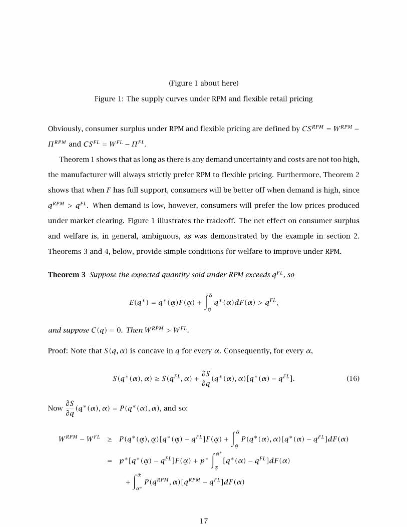
(Figure 1 about here)

Figure 1: The supply curves under RPM and flexible retail pricing

Obviously, consumer surplus under RPM and flexible pricing are defined by CSRPM = WRPM −

ΠRPM and CSFL = WFL −ΠFL.

Theorem 1 shows that as long as there is any demand uncertainty and costs are not too high,

the manufacturer will always strictly prefer RPM to flexible pricing. Furthermore, Theorem 2

shows that when F has full support, consumers will be better off when demand is high, since

qRPM > qFL. When demand is low, however, consumers will prefer the low prices produced

under market clearing. Figure 1 illustrates the tradeoff. The net effect on consumer surplus

and welfare is, in general, ambiguous, as was demonstrated by the example in section 2.

Theorems 3 and 4, below, provide simple conditions for welfare to improve under RPM.

Theorem 3 Suppose the expected quantity sold under RPM exceeds qFL, so

E(q∗) = q∗(α¯)F(α

¯)+

∫ αα¯

q∗(α)dF(α) > qFL,

and suppose C(q) = 0. Then WRPM > WFL.

Proof: Note that S(q,α) is concave in q for every α. Consequently, for every α,

S(q∗(α),α) ≥ S(qFL,α)+ ∂S∂q(q∗(α),α)[q∗(α)− qFL]. (16)

Now∂S∂q(q∗(α),α) = P(q∗(α),α), and so:

WRPM −WFL ≥ P(q∗(α¯),α

¯)[q∗(α

¯)− qFL]F(α

¯)+

∫ αα¯

P(q∗(α),α)[q∗(α)− qFL]dF(α)

= p∗[q∗(α¯)− qFL]F(α

¯)+ p∗

∫ α∗α¯

[q∗(α)− qFL]dF(α)

+∫ αα∗P(qRPM,α)[qRPM − qFL]dF(α)

17

≥ p∗[q∗(α¯)− qFL]F(α

¯)+ p∗

∫ αα¯

[q∗(α)− qFL]dF(α)

= p∗[E(q∗)− qFL] > 0

The second to last inequality follows from the fact that qRPM ≥ q∗(α) for all α, the fact that

qRPM ≥ E[q∗] > qFL, and the fact that P(qRPM,α) ≥ p∗ for all α ≥ α∗. The last inequality

follows from the fact that qRPM > qFL, so that p∗ > 0. �

Theorem 3 is reminiscent of a standard result, namely that if the total quantity sold under

a single, uniform price is the same or higher than that under price discrimination, then price

discrimination reduces total welfare.30 Think of each state of nature as a separate market. RPM

would correspond to the case of a uniform price, and flexible pricing to price discrimination,

since prices vary across states. Note also that the applicability of Theorem 3 is not limited

to the case where costs are sufficiently low that they can be safely ignored. Indeed it is

straightforward to show that when costs are positive, the hypothesis in the Theorem can be

replaced by [E(q∗)− qFL]p∗ > C(qRPM)− C(qFL).

Our welfare result offers the antitrust authorities guidance about which uses of RPM are

most likely to harm consumers. Since RPM has long been illegal in the United States, any

manufacturer employing the practice must strictly prefer it to the alternative of permitting

the retail market to clear. Hence, by Theorem 2 we know that the manufacturer will ship larger

inventories with RPM. Theorem 3 tells us that welfare is improved unless average inventories

remaining unsold at the end of the demand period exceed the additional retailer orders for

inventory that RPM supports. Excess inventories at the end of the demand period therefore

indicate a source for antitrust concern. Note also that the standard test for the efficiency of

vertical restraints, namely whether use of the restraint increases output, is flawed in this case.

Even though output is always higher under RPM, welfare need not increase unless average

sales rise as well.31

30See Tirole (1988), pp. 137–142.31Since the increased sales in high demand states contribute more to expected welfare than the decreased sales

in low demand states, welfare under RPM can be higher even if expected sales are lower. However, if qFL > qm(α¯)

and the decline is too great in the sense that E[(q∗(α)− qFL)P(qFL,α)] ≤ 0, then WRPM < WFL. This assertion is

18

Theorem 3 is concerned with whether welfare on balance improves as a result of the im-

position of RPM. Given that considerable opposition to RPM has been mounted by consumer

groups, it is important to determine the effects of RPM use on consumers directly. Theorem 4

shows, surprisingly, that consumers can, in fact, benefit on balance from RPM, even though

it denies them the ability to purchase at low market-clearing prices in the event of slack de-

mand. This theorem has the additional advantage over Theorem 3 of not requiring any cost

information.

Theorem 4 Suppose that the average price under minimum RPM is strictly lower than the

average price under flexible pricing. Then consumer surplus and manufacturer profits under

RPM strictly exceed consumer surplus and manufacturer profits under flexible pricing. Hence

RPM results in a Pareto improvement.

Proof:

WRPM −WFL = [S(q∗(α¯),α

¯)− S(qFL,α

¯)]F(α

¯)+

∫ αα¯

[S(q∗(α),α)− S(qFL,α)]dF(α)

−C(qRPM)+ C(qFL)

≥ P(q∗(α¯),α

¯)[q∗(α

¯)− qFL]F(α

¯)+

∫ αα¯

P(q∗(α),α)[q∗(α)− qFL]dF(α)

−C(qRPM)+ C(qFL)

= ΠRPM − qFL[P(q∗(α

¯),α

¯)F(α

¯)+

∫ αα¯

P(q∗(α),α)dF(α)]+ C(qFL)

The above inequality follows from the concavity of S(q,α). (See the proof of Theorem 3.)

proved as follows. Analogous to (16), we have:

S(qFL,α) ≥ S(q∗(α),α)+ P(qFL,α)(qFL − q∗(α)).

Furthermore, the inequality qFL > qm(α¯) implies q∗(α

¯) < qFL, so the above inequality is strict in a neighborhood

of α¯

. Consequently,

WFL −WRPM = E[S(qFL,α)− S(q∗(α),α)]> E[P(qFL,α)(qFL − q∗(α))] ≥ 0.

19

Rearranging, we have

CSRPM ≥ WFL − qFLP(q∗(α¯),α

¯)F(α

¯)− qFL

∫ αα¯

P(q∗(α),α)dF(α)+ C(qFL).

Therefore,

CSRPM − CSFL ≥ ΠFL + C(qFL)− qFLP(q∗(α¯),α

¯)F(α

¯)− qFL

∫ αα¯

P(q∗(α),α)dF(α)

= qFL[P(q∗(α

¯),α

¯)F(α

¯)+

∫ αα¯

P(qFL,α)dF(α)

−P(q∗(α¯),α

¯)F(α

¯)−

∫ αα¯

P(q∗(α),α)dF(α)]> 0.

Thus, CSRPM > CSFL. To show that ΠRPM > ΠFL, observe that if ΠRPM = ΠFL, then by The-

orem 1, we must have qFL = qRPM , so that (contrary to the hypothesis of the theorem) the

average price under both solutions would have to coincide. �

Remark 1 The conclusions of Theorems 3 and 4 continue to hold if the strict inequalities in their

hypotheses are replaced by weak inequalities, provided P(qFL,α¯) > 0.32

Theorem 4 can be used to evaluate the impact of forcing firms to desist from imposing

RPM. If the average price rose as a result, both manufacturer and consumer welfare would be

reduced. The converse of Theorem 4 is not true, however, for RPM could benefit consumers

even if it resulted in a higher average price than under flexible pricing.

It might seem that RPM would typically increase average prices substantially. If prices

increase too much in the sense that E[(P(q∗(α),α)−P(qFL,α))q∗(α)] > 0, then we necessarily

have CSRPM < CSFL. Indeed

CSFL − CSRPM = WFL −ΠFL −WRPM +ΠRPM

= E[S(qFL,α)− R(qFL,α)− S(q∗(α),α)+ R(q∗(α),α)]32Indeed, if q∗(α

¯) < qFL, or if q(α

¯) ≥ q∗(α

¯) > qFL, then since S(q,α) is strictly concave on [0, q(α)], the weak

inequality in (16) can be replaced with a strict inequality. If q∗(α) > q(α), then∂S(q∗(α),α)

∂q= 0, but strict

inequality holds nevertheless.

20

≥ E[P(qFL,α)(qFL − q∗(α))− R(qFL,α)+ R(q∗(α),α)]

= E[(P(q∗(α),α)− P(qFL,α))q∗(α)] > 0.

Theorems 5 and 6 provide demand conditions under which RPM does not raise average prices.

These Theorems apply Theorem 4 and Remark 1 to show that for two extreme cases of demand

uncertainty, additive and multiplicative, RPM raises consumer welfare. Both examples assume

constant marginal costs and a condition ensuring that the solution to the flexible pricing

problem is unique, and that the manufacturer strictly prefers RPM.

Theorem 5 If D(p,α) = α− p, and C(q) = cq, then provided c < E(α)− α¯

and α ≤ 2α¯, any

solution to (11) has WRPM > WFL and CSRPM > CSFL.

Proof: As can be seen from the calculations below, the condition c < E(α) − α¯

ensures that

qFL > qm(α¯) = α

¯/2. The condition qc(α) ≤ qm(α) = α/2 ≤ α

¯= q(α

¯) has two implications.

First, Theorems 1 and 2 imply that qRPM > qFL. Second, since qFL ≤ qc(α) the functionΠFL(q)

is strictly concave over its domain. We will now show that E[P(qFL,α)] = E[P(q∗(α),α)] (See

Remark 1). The first-order condition for qFL is

Rq(qFL,α¯)F(α

¯)+

∫ αα¯

Rq(qFL,α)dF(α)− c = 0,

yielding (α¯− 2qFL)F(α

¯) +

∫ αα¯(α − 2qFL)dF(α) − c = 0, or qFL = a−c

2 , where a = E[α]. Since

P(qFL,α) = α− qFL, we obtain

E[P(qFL,α)] = a− qFL = a+ c2.

Now for the RPM case, observe that any solution to (11) must satisfy α ∈ (α¯, α).33 Since

0 < qRPM < q(α∗), we have Pq(qRPM,α∗) < 0 and Pα(qRPM,α∗) > 0. Equations (19) and (20)

33Since the manufacturer strictly prefers RPM, it must be that α∗ > α¯

. Furthermore, since qRPM ≤ qc(α) ≤qm(α), if α∗ = α we would have p∗ = P(qRPM, α) ≥ pm(α). But then since pm(z) is strictly increasing in z,by lowering the price floor below pm(α), the manufacturer can increase his expected revenues in states below αwithout affecting his receipts in state α, a contradiction.

21

in the Appendix then imply that the following first order conditions must be satisfied:

(α¯− 2p∗)F(α

¯)+

∫ α∗α¯

(α− 2p∗)dF(α) = 0

and ∫ αα∗(α− 2qRPM)dF(α) = c.

Since P(q∗(α),α) = p∗ for α ≤ α∗ and P(q∗(α),α) = P(qRPM,α) for α ≥ α∗, any solution to

(11) must satisfy:

2E[P(q∗(α),α)] = 2p∗F(α∗)+ 2∫ αα∗(α− qRPM)dF(α)

= α¯F(α

¯)+

∫ α∗α¯

αdF(α)+∫ αα∗αdF(α)+

∫ αα∗(α− 2qRPM)dF(α)

= a+ c,

where the second and third inequality follow from the first-order condition for RPM. We con-

clude that E[P(q∗(α),α)] = E[P(qFL,α)]. Note that P(qFL,α¯) > 0, for qFL = q(α

¯) = qm(α

¯)

would imply limq↑qFL dΠFL/dq < 0. Hence by Remark 1, WRPM > WFL and CSRPM > CSFL.

�

Theorem 6 Suppose D(p,α) = α(1 − p) 1β for some β > 0 and C(q) = cq. Suppose also that

c < 1 −∫ αα¯

(αα

)βdF(α) and α ≤ (1 + β) 1

βα¯

. Then any solution to (11) has WRPM > WFL and

CSRPM > CSFL.

Proof: As in the proof of Theorem 5, the condition c < 1 −∫ αα¯

(αα

)βdF(α) ensures that

qRPM > qFL. Similarly, α ≤ (1 + β) 1βα¯

guarantees that the solution to (8) is unique, and that

any solution to (11) has qRPM > qFL. Now P(q,α) = 1−(qα

)β, so thatRq(q,α) = 1−(1+β)

(qα

)β.

Consequently, qFL satisfies

Rq(qFL,α¯)F(α

¯)+

∫ αα¯

Rq(qFL,α)dF(α) = 1− (1+ β)(qFL)β[α¯−βF(α

¯)+

∫ αα¯

α−βdF(α)] = c.

22

Observe now that

E[P(qFL,α)] = 1− (qFL)β[α¯−βF(α

¯)+

∫ αα¯

α−βdF(α)] = 1− 1− c1+ β =

β+ c1+ β.

Since at every price all demand curves have the same elasticity, the optimum minimum RPM

price must be equal to the monopoly price, that is, p∗ = pm = β1+ β . Now Equation (21) in

the Appendix shows that any solution to (11) must satisfy

∫ αα∗Rq(qRPM,α)dF(α) = [1− F(α∗)]− (1+ β)(qRPM)β

∫ αα∗α−βdF(α) = c.

Consequently, since pm = β/(1+ β), we have:

E[P(q∗(α),α)] = pmF(α∗)+∫ αα∗P(qRPM,α)dF(α)

= pmF(α∗)+ (1− F(α∗))− (qRPM)β∫ αα∗α−βdF(α)

= pmF(α∗)+ (1− F(α∗))−[

1− F(α∗)− c1+ β

]

= β+ c1+ β.

As in the proof of Theorem 5, we conclude that E[P(q∗(α),α)] = E[P(qFL,α)] = β+ c1+ β , so

that WRPM > WFL and CSRPM > CSFL. �

Without a functional form for demand, the change in the average price is harder to sign,

but we may still apply Theorem 3 to to show that total surplus is lower under market clearing

than under minimum RPM. Theorem 7 provides one set of sufficient conditions. We assume

that demand uncertainty is multiplicative, so D(p,α) can be expressed as αD(p), P(q,α) can

be expressed as P(qα

), qm(α) can be expressed as αqm, and q(α) can be expressed as αq.

Also let revenue, R(q,α), be denoted as αR(qα

).34

Theorem 7 Suppose D(p,α) = αD(p), C(q) = 0, and F is nondegenerate. Then if αqm ≤ α¯

,

and 2R′′(z)+ zR′′′(z) < 0, we have WRPM > WFL.

34Since R(q,α) = P(q/α)q = α[P(q/α)q/α], we can express revenue as αR(q/α), where R(z) = zP(z).

23

Proof: Since Rqα(q,α) > 0, it follows that R′′(z) < 0. Let h(α;qFL) ≡ R′(qFL

α

). The condi-

tions R′′(z) < 0 and 2R′′(z)+ zR′′′(z) < 0 imply h is strictly increasing and strictly concave

in α.

Let G be a distribution such that F is a mean-preserving spread of G and F 6= G. Then

qFL ≤ qm(α) ≤ q(α¯) and since h is strictly concave and strictly increasing, we have:

R′(qFL

α¯

)F(α

¯)+

∫ αα¯

R′(qFL

α

)dF(α) < R′

(qFL

α¯

)G(α

¯)+

∫ αα¯

R′(qFL

α

)dG(α), (17)

where qFL is the equilibrium inventory in the Flexible-Price Game with the distribution F . Since

the left side of inequality (17) must be zero, and since R′′(z) < 0, the equilibrium inventory

in the Flexible-Price Game with the distribution G, qFL(G), must satisfy qFL(G) > qFL.35 Let

a ≡ α¯F(α

¯) +

∫ αα¯αdF(α), and consider the degenerate distribution, G, in which all mass is

placed on the single point, a. It follows, since F is not degenerate, that qFL(G) > qFL. Also, the

first-order condition implies qFL(G) solves R′(qFL(G)a

)= 0. Therefore qFL(G)/a = qm, so we

have qFL(G) = aqm. Since the family of demand curves D(p,α) is isoelastic at the same price,

and since costs are zero, the minimum RPM solution satisfies p∗ = pm and qRPM = qm(α).

Consequently, E(q∗) = aqm = qFL(G) > qFL. Invoking Theorem 3, we conclude WRPM > WFL.

�

Theorem 4 provides a sufficient condition for retail competition to be destructive because

competition hurts not just overall welfare but even consumer surplus, as compared to allowing

the manufacturer to set a price floor. When will market clearing result in a higher expected

retail price than minimum RPM? Remember that inventories are always weakly higher under

RPM (see Theorem 2). When qRPM > qFL, two effects are at work. First, when demand is low,

the price floor set with minimum RPM results in higher prices than under flexible pricing.

Second, when demand is high enough, the price will be lower under RPM, due to the higher

inventories. Consumers benefit on average when the latter effect dominates sufficiently.

If there is “too much” demand uncertainty, as represented by the distribution F and the

35A similar argument is given in Rothschild and Stiglitz (1971).

24

demand functionD(p,α), the retail price in the Flexible-Price Game will be zero in low demand

states. When the manufacturer considers inducing a higher quantity of inventories to be

demanded, revenues are not hurt in low demand states. In effect, the manufacturer ignores

the low demand states, focusing on the high demand states. Under RPM, the price floor binds

and causes the retail price to be well above zero in low demand states. Since inventories will

be discarded when demand is low, the inventory decision is determined by the high demand

states. Induced inventories and prices would be almost the same under market clearing and

RPM in high demand states, so overall expected prices would be higher under RPM. Notice that

this case requires extremely low demand to be unlikely enough for the manufacturer to allow

the retail price to be zero, but requires extremely low demand and a binding price floor to be

likely enough to make the average price under RPM higher than that under market clearing.

Thus, retail competition is most likely to be “destructive”—Pareto-dominated by the alternative

of minimum RPM—when demand fluctuations are moderate. If demand fluctuations are so

great that “fire sales” are likely to occur unless prohibited by RPM, consumers will prefer

flexible pricing. If demand fluctuations are sufficiently small, then the manufacturer will not

impose a binding price floor, so flexible pricing and RPM yield the same outcome.

When fixed production costs are introduced, retail competition can be destructive for a

new reason. Since manufacturer profits, not including fixed costs, are higher under RPM, the

manufacturer may be willing to serve the market under RPM but not under flexible pricing.

Corollary 1 (to Theorem 1): Extend both games by having the manufacturer first choose

whether or not to pay a fixed cost and enter the market. Suppose that F is not a degener-

ate distribution and that when fixed costs are zero we have qFL > qm(α¯). Then there is a range

of fixed costs for which the manufacturer will enter the market when minimum RPM is allowed

but will not enter the market under flexible pricing.

This Corollary corresponds to the ultimate destructive competition. Under flexible pricing,

fixed costs are too high to support nonnegative profits for the manufacturer, so the market

is not served and no surplus is generated. If instead the manufacturer is allowed to set a

25

price floor, then the market is profitable, the manufacturer serves the market, and everyone

benefits.36

This paper has shown that imposing a retail price floor may yield higher profits to the

manufacturer and higher surplus to consumers compared to market clearing. One potential

explanation for the inferiority of market clearing is that markets are incomplete. Under flexible

prices, consumers face price risk, and there are no markets before the realization of demand

on which consumers could trade contingent claims. However, assuming that consumers have

quasilinear utility (thereby justifying our use of consumer surplus as an indicator of their

economic welfare), it is not hard to show that in the absence of market power, market clearing

is Pareto optimal. The intuition is that, under the quasi-linear specification, consumers are

risk neutral with respect to numeraire consumption. If we completed the markets by allowing

income to be traded across states of nature, no one would be better off.37

The nonoptimality of market clearing therefore stems from the presence of market power,

or more precisely, the upstream manufacturer’s unwillingness or inability to employ marginal

cost pricing. In our model, this is a consequence of our assumption that the manufacturer

is a monopolist manipulating the wholesale price. Suppose instead that the manufacturer

had declining average costs and was required to serve all demand by retailers at a wholesale

price equal to average cost. In this context as well, imposing a retail price floor could improve

welfare over a flexible retail price.

5 Summary and Conclusions

We have shown that a monopoly manufacturer selling to uncertain consumer demand through

a competitive retail sector will often wish to impose resale price maintenance on its retailers

in preference to permitting the retail market to clear ex post. Surprisingly, consumers also

36While we have modeled the manufacturer as a monopolist, the inefficiency we identify persists in the presenceof competition between manufacturers as long as the wholesale price remains above marginal cost. Hence therewill be a unilateral incentive to introduce RPM when manufacturers compete, particularly when the manufacturers’brand names are well regarded by consumers.

37This argument has probably been made by other authors, and is formalized in an earlier version of this paper.After a careful specification of the states of nature, the result is immediate.

26

may benefit from the manufacturer’s ability to impose this vertical restraint, as they see lower

prices and greater product availability in the event of high demand. The primary requirement

for RPM to be desirable to all parties is that demand fluctuations not be so great as to cause

catastrophic (to the manufacturer and its retailers) consequences in the event of slack demand.

But even when consumers prefer flexible prices, RPM is desirable to the manufacturer because

it prevents large price fluctuations which would otherwise have impaired inventory holding.

Our model applies best to products satisfying the following criteria:

i. competitive retailers must order inventories prior to the resolution of significant demand

uncertainty;

ii. when RPM is not imposed, retail prices adjust quickly to demand shocks, thereby clearing

the market; and

iii. the products in question have little scrap value, and are expensive to hold for future

demand periods.

For products satisfying criteria i-iii, our model makes the following predictions:

a. Manufacturers prefer RPM to market clearing. Other things equal, orders for inventory

are higher under RPM than under market clearing.

b. Under market-clearing pricing, retail prices and markups are correlated positively with

shocks to demand conditions and retail sales revenues.38

The experience of Nintendo, a leading manufacturer of video game players and cartridges,

provides a particularly apt illustration of our model. Nintendo introduced its game player

and games to the U.S. in the mid-1980’s, a very difficult time to induce retailers to stock such

products.39 Retailers had incurred very large losses on a previous generation of video games.

38While it might seem obvious that an unexpectedly good holiday season should lead to high retail prices, orfewer markdowns, Julio J. Rotemberg and Garth Saloner (1986) have argued in booms, implicit collusion is harderto maintain, so that lower prices prevail. They cite evidence to suggest that markups are countercyclical. Ourmodel predicts that for products satisfying criteria i-iii, markups should be higher when the market in questionexperiences a boom.

39The discussion of Nintendo’s experience is based on a detailed account of the history of Nintendo in DavidSheff (1994).

27

In the early 1980’s, video games had enjoyed phenomenal success, with sales rising from

about $200 million in 1978 to one billion dollars in 1981 and further to three billion dollars in

1982. Excessive inventories resulted in massive price cutting soon after, so that in 1983, sales

fell precipitously to $100 million and the leading manufacturer of games and game players,

Atari, collapsed. The decline in revenues was entirely due to price cutting—unit sales actu-

ally increased. Because retailers ended up holding worthless inventory, they were obviously

reluctant to stock the products of an untested (in the U.S.) video game manufacturer.40

The characteristics of the video game market fit our model well. Games are ordered for

inventory in the late winter and delivered to retailers in the following summer. Nintendo devi-

ated from the standard toy market practice of offering December 10 invoice dating (payment

for goods added to inventories in summer was deferred until cash came in during the holi-

days) by demanding payment within ninety days of shipment, thereby ensuring that the cost

of inventories to retailers was sunk. Most sales occur in the winter holiday season. The Atari

experience proved how sensitive prices were to an excess of available supplies over the quan-

tity demanded. Finally, since new games were introduced each year, scrap value was small.

Accordingly, we should find that Nintendo tried to protect retail prices in order to promote

adequate inventory holding. Initially, Nintendo prevented price cutting by accepting returns

of unsold merchandise (Sheff, 1994, p. 166), but once it obtained a retail foothold, it relied on

controlling inventories and cutting off dealers who cut suggested prices to keep price cutting

from breaking out. These practices resulted, in 1991, in the signing of a consent decree under

which Nintendo agreed not to maintain resale prices of any of its products. Under investi-

gation for RPM, Nintendo had been unable to enforce resale prices during the 1990 holiday

40Consider the following, from Sheff (1994, p.158–9):

“The reason I have this terrific job,” a buyer for the toy company began, “is that the guy before mewas fired after he lost so much in video games. Do you think there is any way I’m going to makethat mistake?”

Throughout 1984, Arakawa [a Nintendo executive] heard variations on that theme over and over whenhe met with toy- and department-store representatives to tell them he was considering entering thehome video-game business. They thought he was nuts.

Arakawa marveled at the intensity of the hostility toward video games—even the phrase was taboo.In the horror stories about the industry, hyperbole was unnecessary. . .

Nintendo’s early efforts to introduce its machines, already very successful in Japan, into the U.S. market failedbecause retailers would not stock inventories (Sheff, 1994, p. 191ff.).

28

season. Influenced by uncertainties surrounding events in Iraq and Kuwait, the 1990 holi-

day season was a slack demand period. The result of slack demand combined with Federal

and state scrutiny of potential RPM was sharp declines in prices of some of Nintendo’s most

popular titles.41

Previous RPM theories do not seem applicable to Nintendo’s use of RPM. Nintendo was

not involved in a manufacturer cartel, and given the range of retail outlets carrying Nintendo

products, a dealer cartel seems distinctly implausible. Efficiency explanations for RPM, such

as pre-sale services (Telser, 1960) and quality certification (Marvel and McCafferty, 1984),

also appear inapplicable.42 We believe that our theory of destructive competition is capable

of explaining RPM use for products for which pre-sale, free-rideable services are difficult to

discern.43 But even for products for which efficiency theories can be applied, our theory

provides a complementary explanation.44

Our goal has been to show that market-clearing pricing need not dominate minimum RPM

when a monopoly manufacturer selling through a competitive retail sector must produce and

ship its product prior to the resolution of demand uncertainty. Our results provide surpris-

ing support for the common claim that RPM is a device desirable for its ability to suppress

destructive competition. At the same time, we have shown that the use of RPM will be most

attractive to manufacturers when demand uncertainty leads to the prospect of deep price cut-

ting in the event of slack demand. It is no surprise, then, that consumer and producer groups

have been deeply divided over the merits of RPM.

Appendix

Let qFL be any solution to (8). Define α0 ≡ inf{z ∈ [α¯, α] : q(z) ≥ qFL}. Note that α0 is well

41See William G. Flanagan and Evan McGlinn, “The Sunny Side of the Recession,” Forbes, January 7, 1991, p. 298:“Nintendo’s popular Zelda game is $19.95 this year at Toys ‘R’ Us, versus $40 last Christmas.”

42Note that leading Nintendo retailers did not offer pre-sale services. In 1991, Toys ‘R’ Us captured 22% of theU.S. toy market. Nintendo sales were approximately 20% of its revenues. K-Mart and Wal-Mart, discount retailers,captured about 10% each of the toy market and were also leading Nintendo retailers. None of these retailersappears to offer the package of services and reputation that in other instances has resulted in RPM use.

43For catalogs of products to which RPM has been applied, see Overstreet (1983) and Ippolito (1988).44Our model of minimum RPM is consistent with Ippolito’s (1991) result that empirically, RPM consists predom-

inantly of enforcement of minimum resale prices.

29

defined, since qFL ≤ qm(α) < q(α). Also, let ∆F(α0) = F(α0)− limz↑α0 F(z) and define

ϕ(q) = R(q,α0)∆F(α0)+∫ αα0

R(q, z)dF(z)− C(q).

Given qFL, α0 is the lowest demand state above which the market-clearing price is positive,

and ϕ(q) represents profits in those states not less than α0. We first establish the following

auxiliary result, which will be used in the proof of Theorem 2.

Lemma 1 The function ϕ(q) is strictly concave on [0, q(α0)], and qFL = arg maxq≤q(α0) ϕ(q).

Proof: Suppose there existed q ≤ q(α0) such that ϕ(q) > ϕ(qFL). Then we would have

ΠFL(q) ≥ϕ(q) > ϕ(qFL) = ΠFL(qFL), contradicting the fact that qFL solves (8). Next, observe

that for all q ∈ (0, q(α0)) and all z ∈ [α0, α], we have R(q, z) ≥ R(q,α0) > 0. Thus, ϕ is a

strictly concave function on [0, q(α0)], and qFL uniquely maximizes ϕ(q). �

Proof of Theorem 2: If qFL = 0, then the result is obvious. Hence suppose that qFL > 0, and

that contrary to the statement of the theorem, there exist solutions to (8) and (11) for which

qRPM < qFL.

Case 1: α0 < α∗. We have

ϕ′(qRPM) = Rq(qRPM,α0)∆F(α0)+∫ αα0

Rq(qRPM, z)dF(z)− C′(qRPM). (18)

We claim thatα∗ ∈ (α¯, α). Since we are in case 1, we know thatα∗ > α

¯. Furthermore, for qRPM

to be an equilibrium inventory for the RPM Game, qRPM ≤ qm(α) must hold. If α∗ = α, we

would have p∗ ≥ P(qRPM,α∗) ≥ pm(α). The last inequality cannot be strict, for then the price

floor would exceed the revenue-maximizing price in every state. But qRPM = qm(α) implies

qFL > qm(α), contradicting the optimality of qFL. Thus, α∗ ∈ (α¯, α).

While Π(q,α) is not necessarily differentiable, it can nevertheless be shown that if α ∈

(α¯, α), we must have

∂Π∂q(qRPM,α∗) = {Rp(P(qRPM,α∗),α

¯)F(α

¯)+

∫ α∗α¯

Rp[P(qRPM,α∗), z]dF(z)}Pq(qRPM,α∗)

30

+∫ αα∗Rq(qRPM, z)dF(z)− C′(qRPM) = 0 (19)

∂Π∂α(α∗, qRPM) = {Rp(P(qRPM,α∗),α

¯)F(α

¯)

+∫ α∗α¯

Rp[P(qRPM,α∗), z]dF(z)}Pα(qRPM,α∗) = 0 (20)

If qRPM = 0, then ΠFL = 0, so q = 0 is a solution to the Flexible-Price Game. Since qFL > 0

is also a solution, this contradicts the fact that qFL uniquely maximizes ϕ(q) on the interval

[0, q(α0)]. Thus, 0 < qRPM < q(α∗), which implies Pq(qRPM,α∗) < 0 and Pα(qRPM,α∗) > 0.

Hence (19) and (20) yield

∫ αα∗Rq(qRPM, z)dF(z)− C′(qRPM) = 0. (21)

Forp∗ to be an equilibrium price floor, p∗ = P(qRPM,α∗) ≤ pm(α∗) holds, and soRq(qRPM,α∗) ≤

0. Since Rqα > 0, we have qm(α¯) ≤ qm(α∗) < qRPM < qFL ≤ q(α0) so that Rq(qRPM, z) is well

defined for all z ∈ [α0, α∗] and satisfies Rq(qRPM, z) ≤ 0 for all z ≤ α∗. Thus (18) and (21)

imply

ϕ′(qRPM) = Rq(qRPM,α0)∆F(α0)+∫ α∗α0

Rq(qRPM, z)dF(z) ≤ 0. (22)

Since qRPM < qFL, andϕ is strictly concave on 0, q(α0)], this contradicts the optimality of qFL.

Case 2: α0 ≥ α∗. We have

ΠFL ≥ R(qRPM,α¯)F(α

¯)+

∫ αα¯

R(qRPM, z)dF(z)− C(qRPM)

≥∫ αα∗R(qRPM, z)dF(z)− C(qRPM)

≥∫ αα∗R(qFL, z)dF(z)− C(qFL) = ΠFL (23)

The third inequality in (23) follows from the fact that qRPM maximizes∫ αα∗ R(q, z)dF(z)−C(q).

The equality in (23) holds because R(qFL, z) = 0 for z ≤ α0. Therefore, all inequalities in (23)

31

must hold as equalities, and so:

∫ αα∗R(qRPM, z)dF(z)− C(qRPM) =

∫ αα0

R(qFL, z)dF(z)− C(qFL). (24)

Now p∗ = P(qRPM,α∗) ≤ pm(α∗), for otherwise the price floor would strictly exceed the

revenue-maximizing price in every state in which the price floor binds, which would be incon-

sistent with equilibrium. Furthermore, the price floor must strictly bind in some states, for

otherwise ΠRPM = ΠFL, and hence by Theorem 1 we would have qRPM = qFL (see note 28).

Consider the following deviation in the RPM Game. Keep the price floor at p∗, but raise

inventories from qRPM to qFL. Let α∗∗ be defined by α∗∗ = sup{z ∈ [α¯, α] : P(qFL, z) < p∗}.

Since p∗ > 0, we have α∗∗ > α0 ≥ α∗. Under this deviation, the manufacturer’s profit would

be:

R(p∗, α¯)F(α

¯) +

∫ α∗∗α¯

R(p∗, z)dF(z)+∫ αα∗∗R(qFL, z)dF(z)− C(qFL)

≥ R(p∗, α¯)F(α

¯)+

∫ α0

α¯

R(p∗, z)dF(z)+∫ αα0

R(qFL, z)dF(z)− C(qFL)

=∫ α0

α∗R(p∗, z)dF(z)+ΠRPM. (25)

The inequality in (25) follows from the fact that for z ∈ (α∗, α∗∗], we have P(qFL, z) ≤ p∗ ≤

pm(α∗) ≤ pm(z) and so R(qFL, z) ≤ R(p∗, z). The equality in (25) holds because of (24).

If the last integral in (25) is strictly positive, we will have contradicted the optimality of

qRPM . To show this, first note that R(p∗, z) > 0 for z ∈ (α∗, α0]. If µ((α∗, α0]) = 0, then

(24) would imply that qRPM and qFL both maximize ϕ(q), contradicting Lemma 1. Therefore

µ((α∗, α0]) > 0, proving the contradiction. We conclude that α0 ≤ α∗ is also inconsistent

with qRPM < qFL.

Furthermore, suppose that the manufacturer strictly prefers RPM, and that either F has

full support or qc(α) ≤ q(α¯), but that contrary to the hypothesis of the theorem,

qRPM = qFL. Note that since qFL ≤ qc(α), the condition qc(α) ≤ q(α¯) implies α0 = α

¯.

Since the manufacturer strictly prefers RPM, the price floor must be strictly binding, so

32

that p∗ = P(qRPM,α∗) > P(qFL,α¯) ≥ 0, implying α∗ > α0 ≥ α

¯. Now if α∗ = α, we would have

qRPM = qm(α), as shown in Case 1 above. Since Rqα > 0 we would then have Rq(qRPM, z) <

Rq(qRPM, α) = 0 for all z ∈ [α0, α). Consequently, since either α0 = α¯

or F has full support,

it follows from (18) that ϕ(qRPM) < 0, contradicting qRPM = qFL. SImilarly, if we had α∗ < α,

then since α∗ > α0 ≥ α¯

, it follows from (22) that ϕ′(qRPM) < 0, again contradicting qRPM =

qFL. �

References

Baumol, William J.; Panzar, John C. and Willig, Robert D. Contestable Markets and the Theory

of Industry Structure. New York: Harcourt Brace Jovanovich, 1982.

Butz, David A. “Vertical Price Controls with Uncertain Demand.” Working Paper, University of

California, Los Angeles, August 1993.

Dana, James D., Jr. “Equilibrium Price Disperson under Demand Uncertainty: The Roles of

Costly Capacity and Market Structure.” Working Paper, University of Chicago, September

1993.

Deneckere, Raymond; Marvel, Howard P. and Peck, James. “Demand Uncertainty, Inventories,

and Resale Price Maintenance.” Working paper, the Ohio State University, October 1995.

Eichner, Alfred S. The Emergence of Oligopoly. Baltimore: Johns Hopkins, 1969.

Hovenkamp, Herbert. “The Antitrust Movement and the Rise of Industrial Organization.” Texas

Law Review, November 1989, 68), pp. 105–67.

Ippolito, Pauline M. Resale Price Maintenance: Economic Evidence from Litigation. Bureau of

Economics Staff Report to the Federal Trade Commission, April 1988.

.“Resale Price Maintenance: Empirical Evidence from Litigation.” Journal of Law & Eco-

nomics, October 1991, 34(2), pp. 263–94.

Lief, Alfred. It Floats: The Story of Procter & Gamble. New York: Rinehart, 1958.

McCraw, Thomas K. Prophets of Regulation, Cambridge: Belknap/Harvard, 1984.

33

Marvel, Howard P. “The Resale Price Maintenance Controversy: Beyond the Conventional Wis-

dom.” Antitrust Law Journal, Fall 1994, 63(1), pp 59–92.

Marvel, Howard P. and Stephen McCafferty. “Resale Price Maintenance and Quality Certifica-

tion.” Rand Journal of Economics, Autumn 1984, 15(3), pp. 346–359.

Marvel, Howard P. and James Peck. “Demand Uncertainty and Returns Policies.” International

Economic Review, August 1995, 36(3), pp. 691–714.

Overstreet, Thomas R., Jr. Resale Price Maintenance: Economic Theories and Empirical Ev-

idence. Bureau of Economics Staff Report to the Federal Trade Commission, November

1983.

Rey, Patrick and Tirole, Jean. “The Logic of Vertical Restraints.” American Economic Review,

December 1986, 76(5), pp. 921–939.

Rothschild, Michael and Stiglitz Joseph E. “Increasing Risk II: Its Economic Consequences.”

Journal of Economic Theory, March 1971, 3(1), pp. 66–84.

Rotemberg, Julio and Saloner, Garth. “A Supergame-Theoretic Model of Price Wars During

Booms.” American Economic Review, June 1986, 76(3), pp. 390–470.

Sheff, David. Game Over: How Nintendo Conquered the World. New York: Vintage, 1994.

Telser, Lester G. “Why Should Manufacturers Want Fair Trade?” Journal of Law & Economics,

October 1960, 3, pp. 86–105.

Tirole, Jean. The Theory of Industrial Organization. Cambridge, Ma.: MIT Press, 1988.

Zerbe, Richard. “The American Sugar Refinery Company, 1887-1914: The Story of a Monopoly.”

Journal of Law & Economics, October 1969, 12(2), pp. 339–375.

34

Quantity

Price

0 qRPMqFL

SRPMSFL

pm