Demographic and Geographic Determinants ofRegional Physician Supply

(preliminary version)

Michael Kuhn� Carsten Ochseny

February 27, 2009

Abstract

We provide a theoretical framework which allows us to analyse howphysician supply at regional level depends on demographic (popula-tion size, age structure, mobility and fertility rates) and geographicdeterminants. Using regional data for Germany, we estimate the rela-tionship between physician supply and the population share of 60plus(20minus), population �ows and a rurality index, also controlling forspatial interactions. We �nd that physician supply is related negativelyto the population share of 60plus within rural areas and positively topopulation growth (due to migration or fertility). In addition, spatialinteractions are signi�cant and positively related to regional physiciansupply..

Keywords: age structure, physician supply, regional population ageing,regional migration, panel data.

JEL classi�cation: I11, J44, J10, R23, C23

�Vienna Institute of Demography; Correspondence: Michael Kuhn,Vienna In-stitute of Demography, Wohllebengasse 12-14, A 1040 Vienna, Austria, e-mail:michael.kuhn@oeaw.ac.at

yUniversity of Rostock; Correspondence: Carsten Ochsen, Department of Eco-nomics, University of Rostock, Ulmenstrasse 69, 18057 Rostock, Germany, e-mail:carsten.ochsen@uni-rostock.de

1

1 Introduction

Population ageing is widely expected to come with an increased per capitademand for (ambulatory) physician services. Everything else equal regionswith high population shares of old persons should then be particularly at-tractive on economic grounds for the location of physician practices andshould therefore exhibit high physician to population ratios. However, cur-sory evidence suggests that this may not be the case. In Germany it appearsthat many rural regions with a high share of the elderly population are inparticular danger of being under-doctored. Ageing may therefore lead to awidening gap in some regions between a high need for health care and a lowsupply that may well warrant policy intervention. Furthermore, there areconcerns about growing regional disparities in the provision of health care.Generally, however, too little is known yet about how demographic, eco-nomic and spatial features of a region interact as determinants of physiciansupply.

This study uses panel data at regional level to examine the relation-ship between regional physician supply and its demographic and geographicdeterminants. In so doing, we note that demographic developments andgeographical location imply a framework with both an intertemporal and aspatial dimension. Given that physicians�location choices are mostly long-term decisions, the intertemporal aspect implies that not only the currentpopulation structure will matter but also the expected population. In as faras they constitute measures of population change, we would therefore expectnet population growth (births �deaths) and net migration to constitute sig-ni�cant determinants for physician supply besides the population and its agestructure in of themselves. Furthermore, we would expect that spatial inter-actions in terms of physician density are important. More speci�cally, ourhypothesis is that the propensity to locate in a particular region is positivelyrelated to the physician density in neighbouring districts. This is becausehigh densities of physicians in neighbouring regions are likely to be associ-ated with strong competition. In turn, this would imply a greater relativeattractiveness for the region under consideration. Finally, we adopt the hy-pothesis that demographic and geographic characteristics do not determinein isolation the attractiveness of a region from a physician�s perspective butinteract in a particular way. More speci�cally, we posit that the high de-mand for services by elderly patients may be less attractive for a physicianif it has to be served within a rural context. Long travel times and pooravailability of public transport deter frail elderly patients from attending thephysician�s practice, implying a high demand for home visits as compared toan urban context. Furthermore, due to the long travel times the provisionof home visits is more costly for the physician in rural areas. Thus, a highdemand from old populations may be served at a relatively low cost withinan urban region but only at a high cost within a rural context. Given that

2

the reimbursement system does not fully account for these di¤erences, oneshould expect a positive correlation between age-structure and a measure ofurbanity in its e¤ect on physician supply.

Using annual data for 439 regions at the district level in Germany for theperiod 1995 to 2004 we examine if the share of 60+ in the population a¤ectsthe physician density negatively in rural regions. We control for severalregional characteristics which, according to the literature, are relevant forthe geographical distribution of physician practices. In a �rst step we use a�xed e¤ects panel estimator to analyze the e¤ects of population aging andpopulation shrinking. Following Driscoll and Kraay (1998) we use standarderrors that are robust to heteroskedasticity and spatial correlation. In thenext step we apply a spatial dynamic panel data estimator as suggested byLee and Yu (2007) and Yu et al. (2008), to �nd out if spatial interactionsin physician density are of importance.

It is common to approximate physician location decisions with the physi-cian density (i.e. physicians per capita) at the macro level. However, ifageing at the regional level is intensi�ed by interregional migration, thismeasure could comprise a measurement error, e.g., because younger andolder people exhibit di¤erences in regional mobility. In fact it is observedempirically that younger people leave rural areas more often than older peo-ple. The number of habitants in these regions falls and, hence, the physiciandensity increases for a given number of physicians. At the same time theshare of older people increases and is therefore positively correlated withthe physician density. Given that physicians�location choices are made forthe long term, physician density comprises a measurement error that is ex-pected to be positive. Therefore, we employ the number of physicians as analternative dependent variable not subject to such a bias.

According to the results, physician supply is negatively related to thepopulation share of 60+ within rural areas, while it is not signi�cantlyrelated to the share within urban regions. The e¤ects of the populationsize are signi�cant positive, which is consistent with theory. Hence, popula-tion ageing and shrinking a¤ects physician geographic decisions as expected.Spatial interactions measured in contiguity e¤ects are signi�cantly related tothe number of physicians in the local district. However, the e¤ect is smallerin magnitude than the population e¤ects. Since the speed of populationageing is much faster in rural regions, policy should provide incentives tomove into these regions not only on equity grounds but also because a wors-ening provision of basic goods and services, such as health care, may reduceeven further the development prospects (e.g. by way of job creation) forsuch regions. In addition, many rural regions in East Germany have a ruralcontiguity neighbor, which means that the bene�t from the spatial e¤ectdisappears here.

3

2 Literature

Hingstman & Boon (1989) analyse the regional dispersion of primary healthcare professionals (GPs, dentists, physiotherapists, midwives and pharma-cists) in the Netherlands. Using cross-sectional data, they examine the e¤ectof local earning opportunities (average income, share of elderly, birth rate,population density) and local amenities (share of green belt, distance tonearest training centre) on the aggregated location choices of practicionersas measured by densities (i.e. number of practitioner per capita) within aregion. Within a simple OLS regression, they identify a signi�cant (at 5percent) negative e¤ect of the share of elderly on the densities of all practi-tioners (except midwives). The intuition for this turns on the features of thepayment system. GPs and pharmacists are reimbursed a capitation for eachpublicly insured patient. This turns the elderly into relatively unpro�tablepatients as the relatively high treatment intensities have to be �nanced outof a �xed budget per patient. In contrast, dentists are reimbursed by feefor service. While this renders pro�table the treatment of patients withhigh demand, for dentistry it is the young rather than the hold who requireintensive treatment.

Kraft & v.d. Schulenburg (1986) employ cross sectional data from Switzer-land to estimate jointly various measures of treatment intensity and thephysician density. The share of old patients (55+) has a positive but in-signi�cant impact on physician density.

Kopetsch (2007) uses cross sectional data (yr 2000 reimbursement datafrom KBV combined with German regional statistics INKAR) to estimatevarious measures of treatment intensity each combined with physician den-sity within a 2SLS framework. Here, the share of population 50+ is used inthe density equation and generally has a signi�cant e¤ect for most types ofphysicians, with the exception of psychotherapists.

Using cross-sectional data from German regional statistics (INKAR 2002),Juerges (2007) also obtains a positive impact of the population share 65+on regional physician densities.

[TO BE COMPLETED]

3 Theoretical Framework

In this section we develop a theoretical framework as a basis for organisingand interpreting our empirical �ndings. We consider a set of I regions, in-dexed by i 2 f1; 2; :::Ig : De�ne ki as a set of regional characteristics. Forconcreteness, we will sometimes understand ki to be a (continuous) indexof (increasing) �rurality�. The demographic structure, of each region is de-scribed by, `i; the size of the local population, and by �i 2 [0; 1], the shareof the elderly within a population consisting of two age groups, the old (o)

4

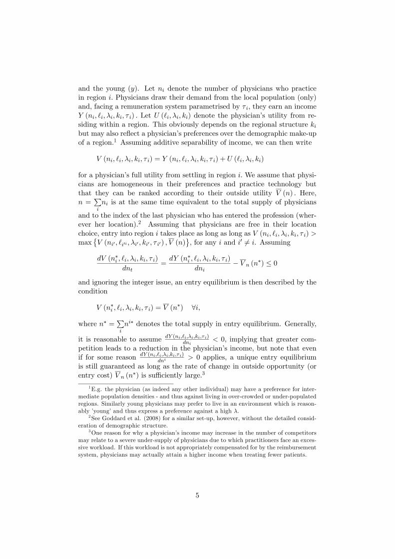
and the young (y). Let ni denote the number of physicians who practicein region i: Physicians draw their demand from the local population (only)and, facing a remuneration system parametrised by � i; they earn an incomeY (ni; `i; �i; ki; � i) : Let U (`i; �i; ki) denote the physician�s utility from re-siding within a region. This obviously depends on the regional structure kibut may also re�ect a physician�s preferences over the demographic make-upof a region.1 Assuming additive separability of income, we can then write

V (ni; `i; �i; ki; � i) = Y (ni; `i; �i; ki; � i) + U (`i; �i; ki)

for a physician�s full utility from settling in region i: We assume that physi-cians are homogeneous in their preferences and practice technology butthat they can be ranked according to their outside utility V (n) : Here,n =

Pini is at the same time equivalent to the total supply of physicians

and to the index of the last physician who has entered the profession (wher-ever her location).2 Assuming that physicians are free in their locationchoice, entry into region i takes place as long as long as V (ni; `i; �i; ki; � i) >max

�V (ni0 ; `i0i ; �i0 ; ki0 ; � i0) ; V (n)

, for any i and i0 6= i. Assuming

dV (n�i ; `i; �i; ki; � i)

dnt=dY (n�i ; `i; �i; ki; � i)

dni� V n (n�) � 0

and ignoring the integer issue, an entry equilibrium is then described by thecondition

V (n�i ; `i; �i; ki; � i) = V (n�) 8i;

where n� =Pini� denotes the total supply in entry equilibrium. Generally,

it is reasonable to assume dY (ni;`i;�i;ki;� i)dni

< 0, implying that greater com-petition leads to a reduction in the physician�s income, but note that evenif for some reason dY (ni;`i;�i;ki;� i)

dni> 0 applies, a unique entry equilibrium

is still guaranteed as long as the rate of change in outside opportunity (orentry cost) V n (n�) is su¢ ciently large.3

1E.g. the physician (as indeed any other individual) may have a preference for inter-mediate population densities - and thus against living in over-crowded or under-populatedregions. Similarly young physicians may prefer to live in an environment which is reason-ably �young�and thus express a preference against a high �:

2See Goddard et al. (2008) for a similar set-up, however, without the detailed consid-eration of demographic structure.

3One reason for why a physician�s income may increase in the number of competitorsmay relate to a severe under-supply of physicians due to which practitioners face an exces-sive workload. If this workload is not appropriately compensated for by the reimbursementsystem, physicians may actually attain a higher income when treating fewer patients.

5

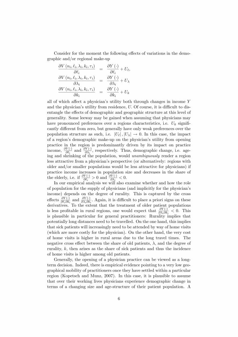
Consider for the moment the following e¤ects of variations in the demo-graphic and/or regional make-up

@V (ni; `i; �i; ki; � i)

@`i=

@Y (�)@`i

+ U`;

@V (ni; `i; �i; ki; � i)

@�i=

@Y (�)@�i

+ U�

@V (ni; `i; �i; ki; � i)

@ki=

@Y (�)@ki

+ Uk

all of which a¤ect a physician�s utility both through changes in income Yand the physician�s utility from residence, U: Of course, it is di¢ cult to dis-entangle the e¤ects of demographic and geographic structure at this level ofgenerality. Some leeway may be gained when assuming that physicians mayhave pronounced preferences over a regions characteristics, i.e. Uk signi�-cantly di¤erent from zero, but generally have only weak preferences over thepopulation structure as such, i.e. jU`j ; jU�j ! 0: In this case, the impactof a region�s demographic make-up on the physician�s utility from openingpractice in the region is predominantly driven by its impact on practiceincome, @Y (�)@`i

and @Y (�)@�i

, respectively. Thus, demographic change, i.e. age-ing and shrinking of the population, would unambiguously render a regionless attractive from a physician�s perspective (or alternatively: regions witholder and/or smaller populations would be less attractive for physicians) ifpractice income increases in population size and decreases in the share ofthe elderly, i.e. if @Y (�)@`i

> 0 and @Y (�)@�i

< 0:In our empirical analysis we will also examine whether and how the role

of population for the supply of physicians (and implicitly for the physician�sincome) depends on the degree of rurality. This is captured by the crosse¤ects @Y (�)

@`i@kiand @Y (�)

@�i@ki: Again, it is di¢ cult to place a priori signs on these

derivatives. To the extent that the treatment of older patient populationsis less pro�table in rural regions, one would expect that @Y (�)

@�i@ki< 0. This

is plausible in particular for general practitioners: Rurality implies thatpotentially long distances need to be travelled. On the one hand, this impliesthat sick patients will increasingly need to be attended by way of home visits(which are more costly for the physician). On the other hand, the very costof home visits is higher in rural areas due to the long travel times. Thenegative cross e¤ect between the share of old patients, �, and the degree ofrurality, k, then arises as the share of sick patients and thus the incidenceof home visits is higher among old patients.

Generally, the opening of a physician practice can be viewed as a long-term decision. Indeed, there is empirical evidence pointing to a very low geo-graphical mobility of practitioners once they have settled within a particularregion (Kopetsch and Munz, 2007). In this case, it is plausible to assumethat over their working lives physicians experience demographic change interms of a changing size and age-structure of their patient population. A

6

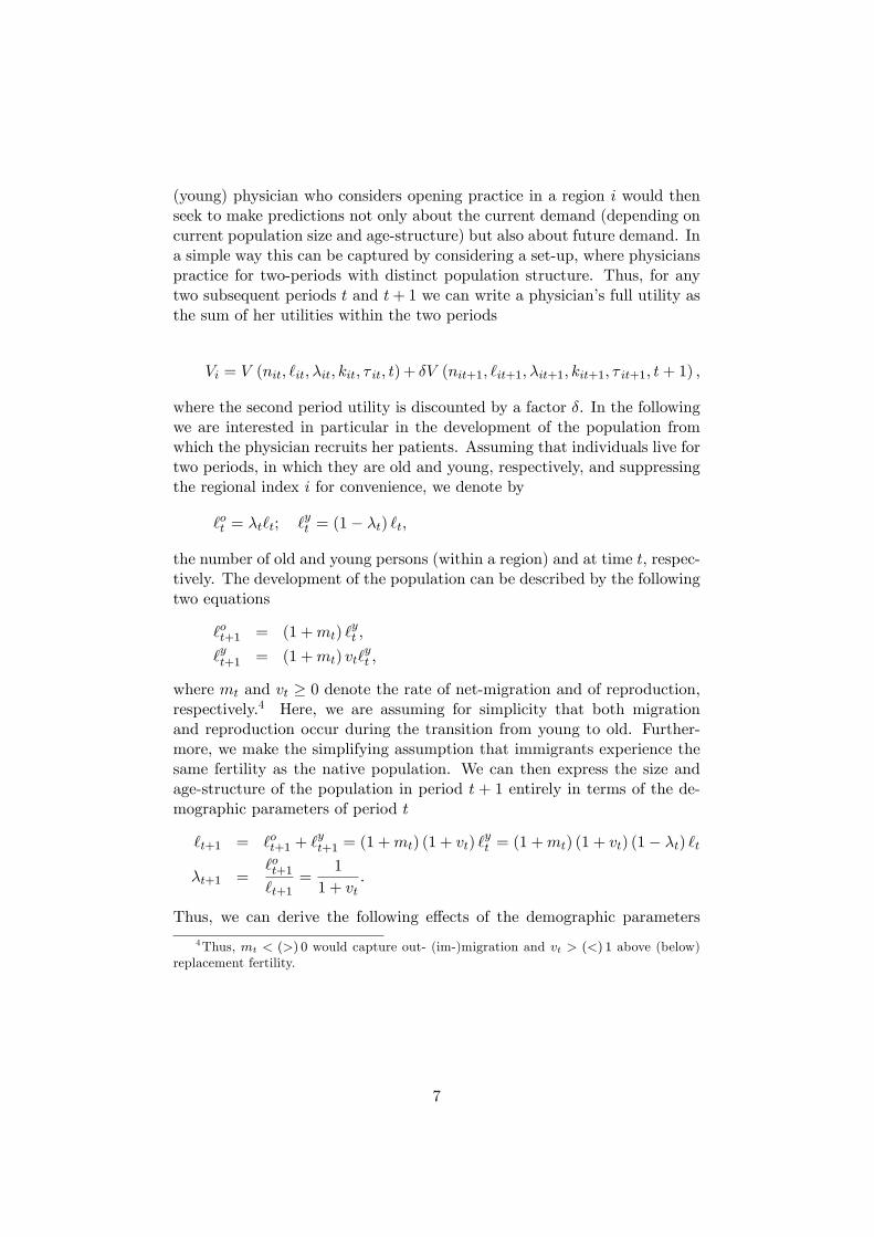
(young) physician who considers opening practice in a region i would thenseek to make predictions not only about the current demand (depending oncurrent population size and age-structure) but also about future demand. Ina simple way this can be captured by considering a set-up, where physicianspractice for two-periods with distinct population structure. Thus, for anytwo subsequent periods t and t+ 1 we can write a physician�s full utility asthe sum of her utilities within the two periods

Vi = V (nit; `it; �it; kit; � it; t) + �V (nit+1; `it+1; �it+1; kit+1; � it+1; t+ 1) ;

where the second period utility is discounted by a factor �. In the followingwe are interested in particular in the development of the population fromwhich the physician recruits her patients. Assuming that individuals live fortwo periods, in which they are old and young, respectively, and suppressingthe regional index i for convenience, we denote by

`ot = �t`t; `yt = (1� �t) `t;

the number of old and young persons (within a region) and at time t, respec-tively. The development of the population can be described by the followingtwo equations

`ot+1 = (1 +mt) `yt ;

`yt+1 = (1 +mt) vt`yt ;

where mt and vt � 0 denote the rate of net-migration and of reproduction,respectively.4 Here, we are assuming for simplicity that both migrationand reproduction occur during the transition from young to old. Further-more, we make the simplifying assumption that immigrants experience thesame fertility as the native population. We can then express the size andage-structure of the population in period t + 1 entirely in terms of the de-mographic parameters of period t

`t+1 = `ot+1 + `yt+1 = (1 +mt) (1 + vt) `

yt = (1 +mt) (1 + vt) (1� �t) `t

�t+1 =`ot+1`t+1

=1

1 + vt:

Thus, we can derive the following e¤ects of the demographic parameters

4Thus, mt < (>) 0 would capture out- (im-)migration and vt > (<) 1 above (below)replacement fertility.

7

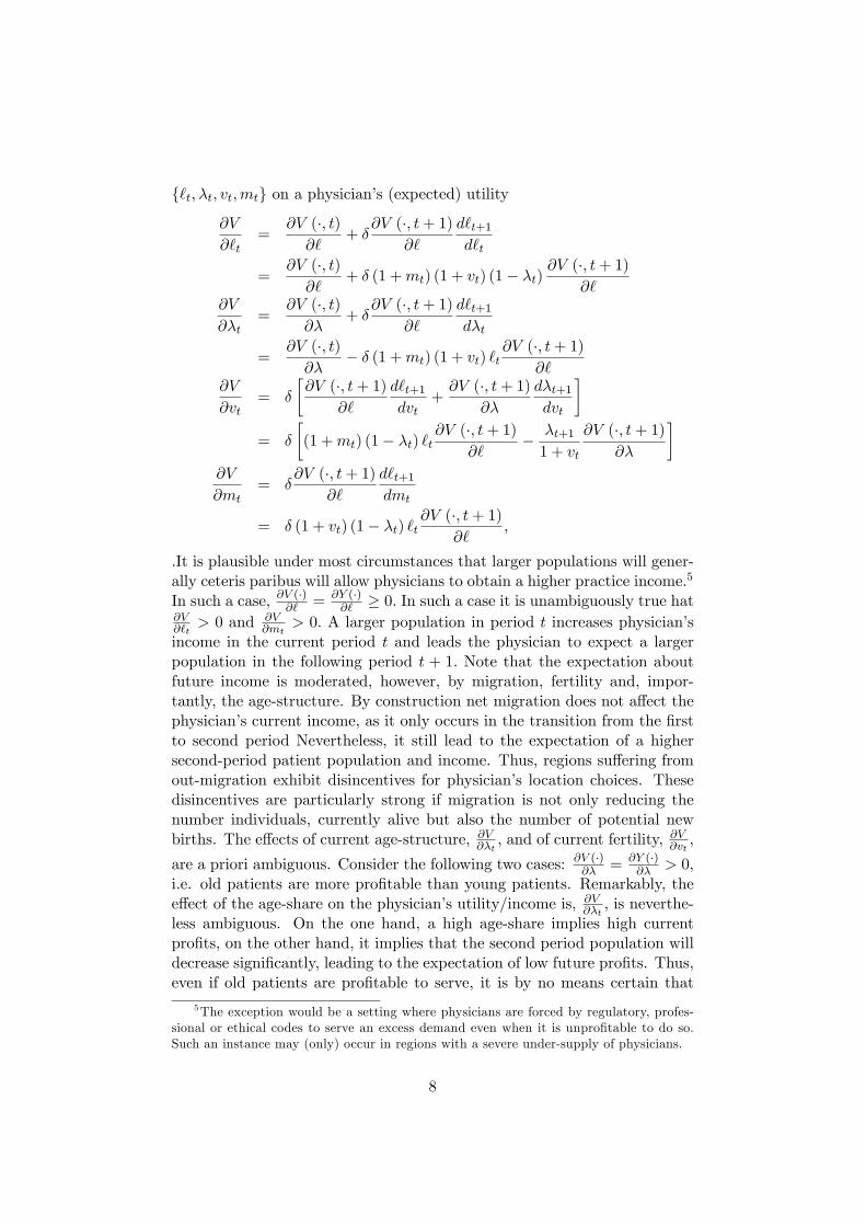
f`t; �t; vt;mtg on a physician�s (expected) utility

@V

@`t=

@V (�; t)@`

+ �@V (�; t+ 1)

@`

d`t+1d`t

=@V (�; t)@`

+ � (1 +mt) (1 + vt) (1� �t)@V (�; t+ 1)

@`@V

@�t=

@V (�; t)@�

+ �@V (�; t+ 1)

@`

d`t+1d�t

=@V (�; t)@�

� � (1 +mt) (1 + vt) `t@V (�; t+ 1)

@`@V

@vt= �

�@V (�; t+ 1)

@`

d`t+1dvt

+@V (�; t+ 1)

@�

d�t+1dvt

�= �

�(1 +mt) (1� �t) `t

@V (�; t+ 1)@`

� �t+11 + vt

@V (�; t+ 1)@�

�@V

@mt= �

@V (�; t+ 1)@`

d`t+1dmt

= � (1 + vt) (1� �t) `t@V (�; t+ 1)

@`;

.It is plausible under most circumstances that larger populations will gener-ally ceteris paribus will allow physicians to obtain a higher practice income.5

In such a case, @V (�)@` = @Y (�)@` � 0: In such a case it is unambiguously true hat

@V@`t

> 0 and @V@mt

> 0: A larger population in period t increases physician�sincome in the current period t and leads the physician to expect a largerpopulation in the following period t + 1: Note that the expectation aboutfuture income is moderated, however, by migration, fertility and, impor-tantly, the age-structure. By construction net migration does not a¤ect thephysician�s current income, as it only occurs in the transition from the �rstto second period Nevertheless, it still lead to the expectation of a highersecond-period patient population and income. Thus, regions su¤ering fromout-migration exhibit disincentives for physician�s location choices. Thesedisincentives are particularly strong if migration is not only reducing thenumber individuals, currently alive but also the number of potential newbirths. The e¤ects of current age-structure, @V@�t ; and of current fertility,

@V@vt;

are a priori ambiguous. Consider the following two cases: @V (�)@� = @Y (�)@� > 0;

i.e. old patients are more pro�table than young patients. Remarkably, thee¤ect of the age-share on the physician�s utility/income is, @V@�t ; is neverthe-less ambiguous. On the one hand, a high age-share implies high currentpro�ts, on the other hand, it implies that the second period population willdecrease signi�cantly, leading to the expectation of low future pro�ts. Thus,even if old patients are pro�table to serve, it is by no means certain that

5The exception would be a setting where physicians are forced by regulatory, profes-sional or ethical codes to serve an excess demand even when it is unpro�table to do so.Such an instance may (only) occur in regions with a severe under-supply of physicians.

8

their presence renders a region attractive from the physician�s perspective.The e¤ect of current fertility on the physician�s utility/income, @V@vt ; is drivenby the expectation of a larger population on the one hand, and a lower age-share, on the other. This leads to an ambiguous e¤ect if old patients arerelatively pro�table. Now, consider a set-up, where old patients are rela-tively less pro�table to serve, @V (�)@� = @Y (�)

@� < 0: In this case, the impact ofcurrent age-share (fertility) on physician income is unambiguously, negative(positive): @V

@�t< 0 ( @V@vt > 0). As it turns out the net e¤ect of ageing on

regional attractiveness for physicians may well depend on the degree of ru-rality. Assuming @Y (�)

@�@k < 0; it is clear that ageing is more likely to renderrural regions unattractive than urban regions. However, the expectation oflower future practice income may imply that ageing triggers a disincentiveto locate even within urban regions, within which it is a priori pro�table toserve an elderly population.

The e¤ect of demographic characteristic xit 2 f`it; �it; vit;mitg on theequilibrium number of physicians n�it can then be found from the followingtotal di¤erential

@Vi@xit

dxit +@Yi (t)

@nitdnit + �

dYi (t+ 1)

dnit+1dnit+1 � V n = 0:

Denoting by bnit the number of young physicians who enter region i in period tand given that all physicians continue their practice within the same regionfor the second period, we have nit = bnit + bnit�1 as the total number ofphysicians in region i in period t: By construction, we then have dnit = dbnit:However, as in period t entry has not yet occurred, we have the forwardlooking expression dnit+1 = dbnit+1 + dbnit. We then obtain the comparativestatic derivative

dn�itdxit

= ��@Vi@xit

+ �dYi (t+ 1)

dnit+1

dbnit+1dxit

��@Yi (t)

@nit+ �

dYi (t+ 1)

dnit+1� V n

��1;

where @Yi(t)@nit

+ � dYi(t+1)dnit+1� V n < 0 holds within an entry equilibrium: Thus,

we have sgndn�it

dxit= sgn

�@Vi@xit

+ � dYi(t+1)dnit+1

dbnit+1dxit

�: The number of physicians

is thus determined both by the direct e¤ect of xit on the physician�s lifetimeutility/income, as was discussed above, and by an e¤ect of the current de-mographic make-up on second-period income as mediated through changesin future physician supply. This latter e¤ect may well be o¤setting, e.g. ifcurrent population growth (1 +mt) vt triggers future entry into the market,or if current ageing, renders future entry unattractive. While it is thus dif-�cult to assign a sign to the comparative static e¤ect, we may assume thatthe e¤ects through changes in competition, are of second-order so that thesign of the overall e¤ect is predominantly determined by the sign of @Vi@xit

; aswas discussed above. Thus, demographic change, i.e. ageing and shrinkingof the population, triggers an unambiguous reduction in physician supply

9

(or alternatively: regions with older and/or smaller populations have fewerphysicians) if practice income and decreases in the share of the elderly, i.e.if dY (�)d`i

> 0 and dY (�)d�i

< 0: At any rate, it was the main purpose of thissection merely to set out a framework for analysis and for understandingthe empirical results to which we shall now proceed.

4 Data

The data used are taken from the INKAR data set provided by the federalo¢ ce for civil engineering and regional development (Bundesamt für Bauwe-sen und Raumordnung). The data are disaggregated to 439 regions at thedistrict level in Germany and cover the period 1995 to 2004. The dependentvariable is the number of physicians. In the robustness section we also usethe number of physicians per 100,000 population . The latter has frequentlybeen used in analyses similar to ours. However, as we will ague below thisvariable exhibits to some extent a measurement bias, and for this reason weprefer to use the number of physicians as dependent variable.

As we have outlined in the previous section, demographic change bearson the regional physician supply population by way of two channels: ageing,in the sense of the age-structure shifting towards higher age-groups, andpopulation decline. Changes in the size of the population are capturedby the �ow variables net migration and the di¤erence between births anddeaths (natural balance) in a region. The size of a population increasesif both variables are positive. Our main interest, however, is in the e¤ectof a changing age structure. We approximate regional population ageingby the population share of people 60 years and older (share 60plus) andthe population share of people 20 years and younger (share 20minus). Aspointed out in the theoretical section, it is possible that the e¤ects of ageingon physician supply vary according to the character of the region (urban vs.rural). We control for these e¤ects by interacting the age groups (60plusand 20minus) with an index of rurality, as provided by the federal o¢ cefor civil engineering and regional development. This index is subaggregatedinto agglomeration areas, municipalized areas, and rural areas. Within thesearea groups there are up to four di¤erent classes di¤ering in population andpopulation density. Altogether there are nine levels of the index, with higherlevels corresponding to a greater degree of �rurality�. See the Appendix forfurther details.

In addition, we use a set of control variables in the estimates. First,we control for the regional population density, measured as population persquare meter, which will be subdivided into population density in East andWest German regions. We do this because a large migration �ow from East-ern to Western regions has taken place in the period under consideration.The remaining set of regional control variables comprise: population size,

10

GDP per capita, unemployment rate, employment rate, share of foreigners,share of welfare recipients, population share of people with a university de-gree, population share of people with at most primary education, share ofnew houses for up to two families and new �ats in the total stock of �ats,tourist accommodation per 100,000 population, and cars per 1,000 popu-lation. We will discuss the expected e¤ects in the next section when wepresent the results.

5 Estimation and Results

In this section we analyze empirically the e¤ects of regional population age-ing and population decline on the regional supply of physicians. In particu-lar, we examine whether the share of older people in the population (60plus)has a di¤erent impact on the supply of physicians in rural regions as opposedto more urban settings.

At the macro level physician supply is usually measured in per capitaterms, i.e. by physician density. However, if ageing at the regional level isintensi�ed by interregional migration, this measure could comprise a mea-surement error. This is possible if, for example, younger and older peopledi¤er in their geographical mobility. It is observed empirically that youngerpeople leave rural areas more often than older people. Outmigration on thepart of the young has two distinct implications for a region. On the one hand,the corresponding decline in population implies that the physician densityincreases for a given number of physicians. At the same time the share ofolder people increases, generating a positive, yet spurious, correlation withphysician density. According to our data physician density is correlated neg-atively with the population share 20minus (�0:57) and positively with thepopulation share 60plus (0:26). Given that physician location choices aremade long term, physician density then comprises a measurement error.

To make this more clear we decompose the physician density (D) intothe real term that is based on decisions of physicians (Y ) and a measure-ment error due to interregional migration (�). The regression that shouldapproximate the true model D = Y + � = � + �X + u + � (with u as idio-syncratic error term) yields a biased parameter � if X and � are correlated.For example, population density and the population share 60plus are cor-related positively (0:13). Since a declining population increases (at least inthe short run) the physician density, we can conclude that the parameterthat corresponds to the share of 60plus is biased negatively. Therefore, inthis section we use only the number of physicians as dependent variable.In the robustness section we run additional regressions with the physiciandensity as dependent variable, conditional on the same set of covariates, toaccount for this bias.

In the theoretical section we have argued that physician supply is, among

11

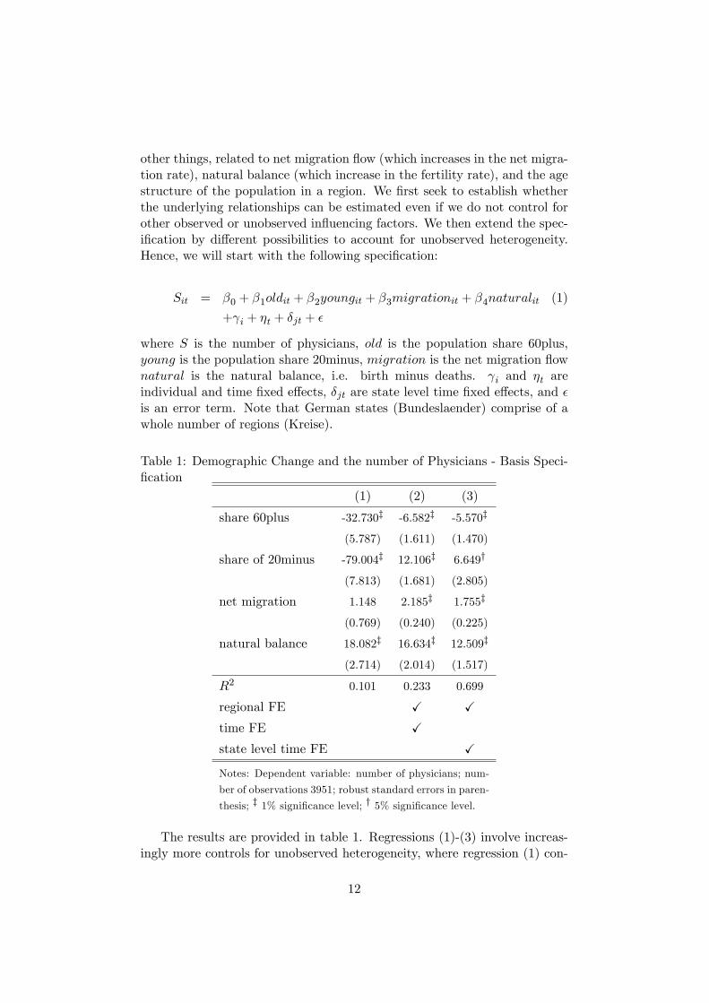
other things, related to net migration �ow (which increases in the net migra-tion rate), natural balance (which increase in the fertility rate), and the agestructure of the population in a region. We �rst seek to establish whetherthe underlying relationships can be estimated even if we do not control forother observed or unobserved in�uencing factors. We then extend the spec-i�cation by di¤erent possibilities to account for unobserved heterogeneity.Hence, we will start with the following speci�cation:

Sit = �0 + �1oldit + �2youngit + �3migrationit + �4naturalit (1)

+ i + �t + �jt + �

where S is the number of physicians, old is the population share 60plus,young is the population share 20minus, migration is the net migration �ownatural is the natural balance, i.e. birth minus deaths. i and �t areindividual and time �xed e¤ects, �jt are state level time �xed e¤ects, and �is an error term. Note that German states (Bundeslaender) comprise of awhole number of regions (Kreise).

Table 1: Demographic Change and the number of Physicians - Basis Speci-�cation

(1) (2) (3)

share 60plus -32.730z -6.582z -5.570z

(5.787) (1.611) (1.470)

share of 20minus -79.004z 12.106z 6.649y

(7.813) (1.681) (2.805)

net migration 1.148 2.185z 1.755z

(0.769) (0.240) (0.225)

natural balance 18.082z 16.634z 12.509z

(2.714) (2.014) (1.517)

R2 0.101 0.233 0.699

regional FE X Xtime FE Xstate level time FE XNotes: Dependent variable: number of physicians; num-

ber of observations 3951; robust standard errors in paren-

thesis; z 1% signi�cance level; y 5% signi�cance level.

The results are provided in table 1. Regressions (1)-(3) involve increas-ingly more controls for unobserved heterogeneity, where regression (1) con-

12

tains no controls at all, regression (2) controls for regional and period �xede¤ects, and regression (3) controls in addition for �xed e¤ects at state level.We consistently �nd that physician supply decreases in the share 60plus andincreases in net migration and the natural balance. This corresponds wellwith our model, according to which population growth, fertility or migra-tion driven, will generally increase the physician�s future demand and, thus,provide incentives to locate within this region. A higher current share ofolder people, certainly leads to the expectation of lower future demand, adisincentive for location. Whether or not the treatment of older patientsis relatively pro�table or not cannot be inferred, only that possible currentpro�ts from treating older patients would be overcompensated by the ex-pectation of future losses in demand and income. The e¤ect of the age share20minus is not robust with respect to changes in speci�cation and changessign from negative to positive once unobserved heterogeneity is controlledfor. From the more reliable estimations (2) and (3) it follows that youngpopulations provide a positive stimulus for physician supply. This may befor young patients being relatively pro�table, but it also embraces the ex-pectation that currently young populations guarantee a high demand wellinto the future. From these simple regressions it follows that both chan-nels of demographic change, namely ageing and population decline, a¤ectsphysician decisions negatively.

In the following we add to elements to our estimation. Firstly, we nowinclude a number of control variables to analyze if the estimated e¤ects ofthe demographic change remain signi�cant, if other determinants of physi-cian supply are considered. In table 1 we provide standard errors that arerobust to heteroskedasticity and autocorrelation. We now calculate stan-dard errors that are robust to heteroskedasticity and autocorrelation andadditionally robust to contemporaneous cross-sectional correlations in theerror terms following Driscoll and Kraay (1998). According to Driscoll andKraay spatial correlations among cross-sections may arise for a number ofreasons, ranging from observed common shocks such as terms of trade oilshocks, to unobserved contagion or neighborhood e¤ects.6

Secondly, we examine in greater detail the relationship between the de-mographic and geographic make-up of a region. We have argued before, thatin particular the e¤ect of age structure on physicians�location incentives mayimportantly be shaped by the degree of rurality. Therefore we additionallyinclude interactions of the age groups with our proxy for rurality discussedin the data section.

One argument is, that it is more di¢ cult for rural areas to attract or

6According to Driscoll and Kraay (1998) the presence of such spatial correlations inresiduals complicates standard inference procedures that combine time-series and cross-sectional data since these techniques typically require the assumption that the cross-sectional units are independent. When this assumption is violated, estimates of standarderrors are inconsistent, and hence are not useful for inference.

13

retain young people or those in the working age population. Hence, if ageinghappens in these regions it seems to be obvious that this process is not easilyreversed. Furthermore, we have argued in the theoretical section that thedegree of rurality may a¤ect the relative pro�tability of treating di¤erentage-groups. In particular, we have conjectured that the treatment of old- and similarly perhaps for very young - patients within a rural contextarguably involves a larger share of provision by way of house visits. Inparticular in rural areas these are likely to be costly for physician due tolong travelling times.

We now estimate

Sit = �0 + �1oldit + �2oldit � ruralityi (2)

+�3youngit + �4youngit � ruralityi+�5migrationit + �6naturalit + �

0Xit + i + �jt + �

where, in addition to speci�cation (1), we have included the interactionof population share 60plus with the rurality variable (oldit � ruralityi), theinteraction of population share 20minus with the rurality variable (youngit�ruralityi), and a vector of control variables, Xit.

The models presented in table 2 di¤er with respect to the restriction�2 = �4 = 0 in the regression (1). The omission of the interaction termswithin this regression renders the results more comparable with the esti-mates provided in table 1. According to regression (1) ageing a¤ects physi-cian supply negatively, which is accordance with the results presented intable 1. The additional interaction with rurality in regression (2) showsthat the negative e¤ect of the population 60plus on physician supply is par-ticularly pronounced for rural areas. In fact, within an urban context thereverse may well be true, as the pure e¤ect of the share 60plus is now posi-tive, albeit insigni�cant. As the (negative) e¤ect of ageing on the expectedfuture demand should not vary too much with the regional context, thisstrongly hints at the fact that rurality reduces the relative pro�tability oftreating old patients. As is well known from the empirical literature, olderpatients (60plus) exhibit far higher consultation rates and, thus, generate ahigher demand for physicians (see e.g. Pohlmeier and Ulrich 1995, Dusheikoet al. 2002, Dormont et al. 2006, Juerges 2007). Whereas meeting thisdemand appears to be relatively pro�table within an urban context, it isunpro�table within rural settings.

When taken across all regions alike, the share of the young population20minus does not have a signi�cant e¤ect on physician supply (see regression(1)). However, if we consider in addition the interaction with rurality, we�nd that a high share of the young is most attractive in urban regions:whereas the direct e¤ect of the share of 20minus is signi�cantly positive, theinteraction with rurality is signi�cantly negative. The positive direct e¤ect is

14

consistent with a young population being a good indicator for a high futuredemand. The fact that the attractiveness of young patients weakens withinrural areas either hints at the fact that treating the higher demand fromyoung ages within a rural context exposes the physician again to additionalcosts.7 Alternatively, it may hint at the expectation that young populationsmay not stay within rural areas but rather migrate elsewhere. Net migrationand natural balance are signi�cant positive in both speci�cations. These twovariables being proxies for the expected future demand, con�rms once morethat physician supply is driven not only by the size and age-structure of thecurrent population but also by the expectations about future populationstructure.

table 2 about here

The main reason for why we can interpret the two population �ow e¤ectsin terms of expectations is that population size has a signi�cant positive ef-fect in of itself. As such, this is not surprising since the number of physiciansis related to the number of inhabitants in the region. But to the extent thatchanges in population over time are measured directly, a the populationbalance would suggest that one of the three determinates - population size,net migration or natural balance - should turn out to be insigni�cant. Thefact that all three variables are signi�cant then hints at the additional roleof expectation over and above the mere population accounting. In the sub-sequent section on robustness (section 6) we apply a dynamic model thatallows us to conclude whether this e¤ect is important even in the short run.In this case, we argue, that expectations play only a minor role. Further-more, we check in section 6 if the �ow e¤ects disappear, if we choose thephysician density as dependent variable.

We divide the population density e¤ect into West and East because thenet migration �ow between the two subregions is unilateral in the periodconsidered in the estimates. Between 1990 and 2004 the East German pop-ulation has decreased by about 7.5%, while the West German populationhas increased by almost 7%. Hence, within Germany there is East-to-Westmigration, a process which has intensi�ed in the middle of the 1990s. Ac-cording to the literature the e¤ect of population density is positive, becausehigher densities indicate on average, a lower need for travelling either by pa-tients or by physicians and thus a higher demand and/or greater pro�tabilityof provision. One explanation for why the West German e¤ect is not signif-icant is that we control for the share of the elderly in the population, whichare less mobile. With respect to the signi�cant negative e¤ect for East Ger-many we argue that the population density decreases in nearly all regions.

7The studies on the intensity of use of physician services by Pohlmeier and Ulrich(1995), Dusheiko et al. (2002), Dormont et al. (2006) and Juerges (2007) consistentlyreveal a U shaped age-pattern, thus suggesting a relatively high demand for physicianservices both for the old and youngest ages.

15

At face value, this may seem to be a good message, as it would imply thatthe physician density (with reference to population) increases. However,this is simply an arti�cial e¤ect as long as physicians do not abandon theirpractice promptly. Moreover, since the location choice is a long-run decision,in most cases they persevere until they retire. Hence, the results are drivenby a restructuring process.

For the GDP per capita and the employment rate we argue that theyare a proxy for the standard of living and the sound condition of the labormarket. In contrast to this, and in accordance with the literature, the unem-ployment rate and the share of welfare recipients are proxies for morbidity.8.Hence, the e¤ects are expected to be positive. For the share of foreigners we�nd no signi�cant e¤ect, nor for the share of academics. As expected, theshare of those without a formal education a¤ect the number of physicians ina region negatively. In as far as this hints at a relatively poor educationalenvironment, it would reduce the residential utility of physicians who carefor the development of their own children. The two variables that measurethe development of new buildings for living should capture the attractive-ness of regions. The share of new houses is related only to one and twofamily houses and is therefore directly related to an increase in the num-ber of families. The share of new �ats in the stock of �ats measures thegeneral activities of housebuildung. In as far as such construction activitieshint at the simultaneous development of a regional infrastructure (schools,shopping, etc) they provide an additional measure of a region�s attractive-ness. In a far as development is in particular directed at families, this mayprovide an additional hint that such a region may be particularly attractivefor young physicians (upon the point of their location choice). The capacityof tourist accommodation hints at the attractiveness of such a region bothin general and for holiday makers. The e¤ect on physician supply can beexpected to be positive, both because the region is attractive and because ofthe additional demand generated by holiday makers. Finally, cars per 1000population acts as a measure of geographical mobility. On the one hand,mobility should have a positive e¤ect on physician supply: potential patients�nd it easier to visit the physician and, thus, exhibit a greater (expected)contact frequency. On the other hand, given that we control for the popula-tion size and density as well as for the age structure this variable measuresthe possibility to consult physician outside the region, e.g. in order to visita specialist within a city rather than the local general practitioner. In thiscase the expected e¤ect is negative, and this is what we measure.

8See Stewart (2001) for a relatively recent survey on the positive correlation betweenunemployment and morbidity. The fact that direction of causality remains unresolved isimmaterial for our purposes.

16

6 Robustness Check

As mentioned in the previous section, in this section we provide two furthermodels that should help to assess the robustness of our results. In the�rst case we estimate the speci�cations of equation (2), but with physiciandensity as dependent variable. As mentioned in the data section, it is rathercommon in the literature is to use this variable as a dependent instead ofthe number of physicians . The subsequent analysis thus makes our resultsmore comparable with other studies and allows to analyse if our generalconclusions will change. In the second case we estimate a dynamic spatialpanel data model. This allows to consider both short-term e¤ects of thedemographic change in the local area and e¤ects of the market for physiciansin the surrounding regions.

table 3 about here

Using the physician density as dependent variable in equation (2) yieldsthe results displayed in table 3. With respect to the e¤ects of the populationage structure we get comparable results. However, the share of the youngpopulation is no longer signi�cant in regression (2). The population �owvariables, net migration and natural balance, are still signi�cant, althoughthe population size is not considered on the right hand side of the equation.Hence, the general conclusions based on the results presented in table 2 donot change. In addition, we can conclude that the measurement bias in thedependent variable is apparently not large enough to a¤ect our results.

We now turn to the spatial and time dynamic model. In order to generatespatially lagged counterparts of the dependent variable, we construct a spa-tial weight matrix indicating the contiguity of regions. We de�ne contiguitybetween two regions as regions sharing a common border. The correspond-ing spatial weight matrix W is therefore a symmetric 439� 439 matrix. Wis row normalized, which ensures that all weights are between 0 and 1, andweighting operations can be interpreted as an average of the neighboringvalues.

Although we are principally interested in long run e¤ects, we considerthis alternative approach, because it allows us to di¤erentiate between ex-pectations concerning the future and short-term utility/pro�t maximisation.Put di¤erently, we argue that only the latter e¤ect should remain in thisspeci�cation. Usual �xed e¤ects estimators that include spatial and timedynamic e¤ects of the dependent variable are biased.9 Hence, we use aspatial and time dynamic data approach with both regional and time �xede¤ects as suggested by Lee and Yu (2007) and Yu et al. (2008). In this

9See, for example, Nickell (1981) with respect to the asymptotic bias of OLS estimationusing the time lagged e¤ect and, for example, Kelejian and Prucha (1998) for biased OLSestimates when spatial lagged e¤ects are considered.

17

case, the parameters for the time lagged and spatial lagged values of thedependent variables will be estimated using a quasi-maximum likelihood es-timator that is extended by a bias correction. To avoid biased estimates forthe lagged e¤ects of the dependent variables, Lee and Yu (2007) developeda data transformation approach that has the same asymptotic e¢ ciency asthe quasi-maximum likelihood estimator when n is not relatively smallerthan T .

table 4 about here

We apply this estimation technique to equation (2) and choose the num-ber of physicians as well as the physician density as dependent variables.Although we only show the results for the important variables, the spec-i�cation with respect to the remaining control variables has not changed.With respect to the spatial lagged e¤ect of the dependent variable we �nda signi�cant positive e¤ect. This means that the propensity to locate ina particular region is positively related to the physician density in neigh-boring districts. This is because high densities of physicians in neighboringregions are likely to be associated with strong competition there. In turn,this would imply a greater relative attractiveness for the local region underconsideration.

With respect to the age e¤ects we can conclude that the young as wellas the old are negatively associated with rural areas. That is, the higherthe rurality level is the more pro�table is the working age population. Thisis consistent with our previous �ndings. The main di¤erence to the resultsin table 2 is, that the share of young is no longer signi�cant in regression(2). Hence, this e¤ect is driven by expectation about future income. Fornet migration and natural balance we �nd that the estimated e¤ects are notsigni�cant or at least have a lower signi�cance level. According to tables2 and 3, it follows that the population �ows thus measure in fact mainlyexpectations.

7 Conclusions

Population ageing is widely expected to come with an increased per capitademand for (ambulatory) physician services. Everything else equal regionswith high population shares of old persons should then be particularly at-tractive on economic grounds for the location of physician practices andshould therefore exhibit high physician to population ratios.

At the regional level in Germany, ageing is not only shaped by low ordeclining fertility rates but also by outmigration. This is because youngerpeople exhibit a higher regional mobility than older people. Hence, ageingmay be accelerated by outmigration in particular as it becomes progressivelymore di¢ cult to attract young people into regions in which the average

18

age is increasing towards (or at) high levels. According to our data thelargest population share of the age cohort 60plus in 2004 lives in the regionHoyerswerda (33.4%) followed by the region Görlitz (32.9%); two regions inEast Germany. Between 1995 and 2004 the share of 60plus has increased by89% in Hoyerswerda and 41% in Görlitz. However, there are other regions,in particular in the Eastern part of Germany, that experience ageing in asimilar manner. According to the results, physician supply is negativelyrelated to the population share of 60+ within rural areas, while it is notsigni�cantly related to the share within urban regions. Hence, many ruralregions with a high share of the elderly population are in particular danger ofbeing under-doctored in the future, if the identi�ed e¤ects in our regressionsare in fact a causal.

Additionally, we adopt the hypothesis that demographic and geographiccharacteristics do not determine in isolation the attractiveness of a regionfrom a physician�s perspective but interact in a particular way. More specif-ically, we posit that the high demand for services by elderly patients may beless attractive for a physician if it has to be served within a rural context.Long travel times and poor availability of public transport deter frail elderlypatients from attending the physician�s practice, implying a high demandfor home visits as compared to an urban context. Furthermore, due to thelong travel times the provision of home visits is more costly for the physicianin rural areas. Thus, a high demand from old populations may be served ata relatively low cost within an urban region but only at a high cost withina rural context. Given that the interaction of age-related population sharesand the rurality variable (in nine levels) is adequate to measure this e¤ect,we �nd that the share of the elderly has an increasing negative e¤ect onphysician supply, the higher the level of rurality.

At regional level, demographic developments and geographical locationimply a framework with both an intertemporal and a spatial dimension.Given that physicians�location choices are mostly long-term decisions, theintertemporal aspect implies that not only the current population structurewill matter but also the expected population. In fact, we �nd that net pop-ulation growth (births �deaths) and net migration to constitute signi�cantdeterminants for physician supply besides the population and its age struc-ture in of themselves. Furthermore, spatial interactions in terms of physiciandensity are important. More speci�cally, the econometric results con�rm ourhypothesis whereby the propensity to locate in a particular region is pos-itively related to the physician density in neighbouring districts. This isbecause high densities of physicians in neighbouring regions are likely to beassociated with strong competition. In turn, this would implies a greaterrelative attractiveness for the region under consideration.

Unlike the East-West migration ageing did not start in Germany in theearly 1990s but in West Germany has been in e¤ect from the second half ofthe 1970s onwards. We can therefore assume that the estimated e¤ects of re-

19

gional population ageing are robust for Western German regions. However,the East German population density e¤ect on physician supply is underes-timated. In 2007 the share of 50plus among the physicians is 37.7%, whileit was 30.3% in 1997. Hence, ageing happens to physicians, too. From thisit follows that a large number of physicians will retire in the next 15 yearsand this will touch the medical provision particularly in the eastern partof Germany. According to the German Medical Association about 13% ofthe East German regions are medically �underprovided� in 2007. In addi-tion, more than half of the hospitals in East Germany have problems to �llvacancies in medical employment.

The important problem for the future lies in attracting new and youngphysicians to these regions, as it is known from statistical projections thatpopulation decline in many East German regions will go on for the next 20years. Since the speed of population ageing is much faster in rural regions,policy should provide incentives to move into these regions not only on equitygrounds but also because a worsening provision of basic goods and services,such as health care, may reduce even further the development prospects (e.g.by way of job creation) for such regions. In addition, many rural regionsin East Germany have a rural contiguity neighbor, which means that thepositive spatial e¤ect disappears here.

8 References

Dormont, B., Grignon, M., Huber, H., 2006, Health expenditure growth:reasssessing the threat of ageing, Health Economics 15, 947-963.

Driscoll, J.C., Kraay, A.C., 1998, Consistent Covariance Matrix Estima-tion with Spatially Dependent Panel Data, Review of Economics andStatistics 80, 549-560.

Dusheiko, M, Gravelle, H., Campbell, S., 2002, Inequality in Consultationswith General Practitioners, CHE Technical Paper 24.

Hingstman, L., Boon, H., 1989, Regional Dispersion of Independent Pro-fessionals in Primary Health Care in the Netherlands, Social Science& Medicine 28, 121-129.

Juerges, H., 2007, Health Insurance Status and Physician-Induced Demandfor Medical Services in Germany: New Evidence from Combined Dis-trict and Individual Level Data, DIW Discussion Paper 689.

Kelejian, H.H., Prucha, I.R., 1998, Estimation of Spatial Regression Modelswith Autoregressive Errors by Two-Stage Least Squares Procedures: ASerious Problem, International Regional Science Review 20, 103-111.

20

Kopetsch, T., 2007, Arztdichte und Inanspruchnahme aerztlicher Leistun-gen in Deutschland. Eine empirischeUntersuchung der These vonder angebotsinduzierten Nachfrage nach ambulanten Arztleistungen[Physician density and use of physician services in Germany. An empir-ical investigation into the thesisof supplier-induced demand], SchmollersJahrbuch.

Kopetsch, T., Munz, H., 2007, Analyse des Niederlassungs- und Wan-derungsverhaltens von Vertragsaerzten und -psychotherapeuten in Deutsch-land [Analysis of location and migration choices by registered physi-cians in Germany], Berlin: Kassenaerztliche Bundesvereinigung.

Kraft, K., von der Schulenburg, J.-M., 1986, Co-Insurance and Supplier-Induced Demand in Medical Care: What Do We Have to Expect as thePhysician�s Response to Increased Out-of-Pocket Payments, Journal ofInstitutional and Theoretical Economics 142, 360-379.

Lee, L.-F., Yu, J., 2007, A Spatial Dynamic Panel Data Model with BothTime and Individual Fixed E¤ects, Ohio State University, Departmentof Economics, mimeo.

Nickell, S.J., 1981, Biases in Dynamic Models with Fixed E¤ects, Econo-metrica 59, 1417-1426.

Newhouse, J.P., Williams, A.P., Bennett, B.W., Schwartz, W.B., 1982,Does the geographical distribution of physicians re�ect market failure?,Bell Journal of Economics 13, 493-505.

Pohlmeier, W., Ulrich, V., 1995, An Econometric Model of the Two-PartDecisionmaking Process in the Demand for Health Care, Journal ofHuman Resources 30, 339-361.

Stewart, J., 2001, The impact of health status on the duration of unem-ployment spells and the implications for studies of the impact of unem-ployment on health status, Journal of Health Economics 20, 781-796.

Yu, J.; de Jong, R.; Lee, L.-F., 2008, Quasi-Maximum Likelihood Estima-tors for Spatial Dynamic Panel Data with Fixed e¤ects when Both nand T are Large, Journal of Econometrics 146, 118-134.

9 Appendix

21

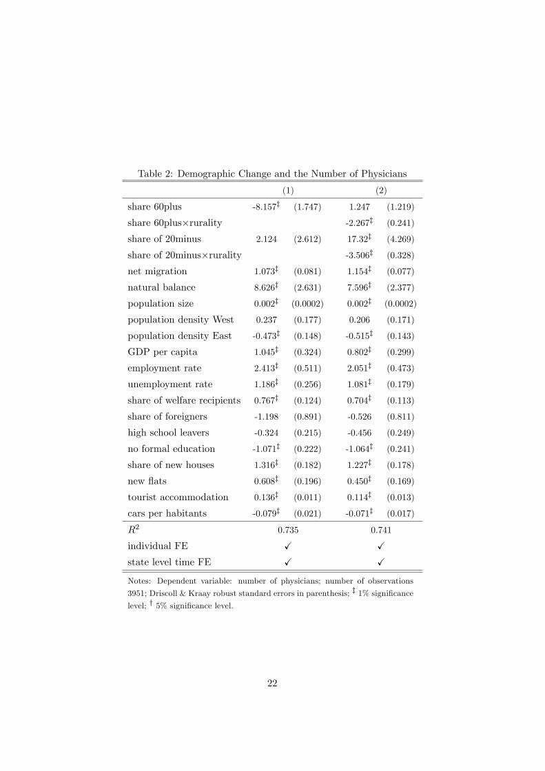
Table 2: Demographic Change and the Number of Physicians

(1) (2)

share 60plus -8.157z (1.747) 1.247 (1.219)

share 60plus�rurality -2.267z (0.241)

share of 20minus 2.124 (2.612) 17.32z (4.269)

share of 20minus�rurality -3.506z (0.328)

net migration 1.073z (0.081) 1.154z (0.077)

natural balance 8.626z (2.631) 7.596z (2.377)

population size 0.002z (0.0002) 0.002z (0.0002)

population density West 0.237 (0.177) 0.206 (0.171)

population density East -0.473z (0.148) -0.515z (0.143)

GDP per capita 1.045z (0.324) 0.802z (0.299)

employment rate 2.413z (0.511) 2.051z (0.473)

unemployment rate 1.186z (0.256) 1.081z (0.179)

share of welfare recipients 0.767z (0.124) 0.704z (0.113)

share of foreigners -1.198 (0.891) -0.526 (0.811)

high school leavers -0.324 (0.215) -0.456 (0.249)

no formal education -1.071z (0.222) -1.064z (0.241)

share of new houses 1.316z (0.182) 1.227z (0.178)

new �ats 0.608z (0.196) 0.450z (0.169)

tourist accommodation 0.136z (0.011) 0.114z (0.013)

cars per habitants -0.079z (0.021) -0.071z (0.017)

R2 0.735 0.741

individual FE X Xstate level time FE X XNotes: Dependent variable: number of physicians; number of observations

3951; Driscoll & Kraay robust standard errors in parenthesis; z 1% signi�cancelevel; y 5% signi�cance level.

22

Table 3: Demographic Change and Physician Density

(1) (2)

share 60plus -1.483z (0.496) -0.472 (0.322)

share 60plus�rurality -0.257z (0.066)

share of 20minus -0.935 (1.600) 2.391 (1.522)

share of 20minus�rurality -0.629z (0.094)

net migration 0.373z (0.036) 0.389z (0.035)

natural balance 2.736z (0.779) 2.698z (0.773)

population density West 0.011 (0.028) 0.007 (0.028)

population density East -0.178z (0.025) -0.188z (0.023)

GDP per capita 0.620z (0.151) 0.606z (0.157)

employment rate 0.277] (0.164) 0.220 (0.163)

unemployment rate 0.421z (0.090) 0.364z (0.079)

share of welfare recipients 0.078y (0.038) 0.072y (0.038)

share of foreigners 1.092z (0.178) 1.181z (0.190)

high school leavers 0.076 (0.094) 0.070 (0.098)

no formal education -0.050 (0.070) -0.049 (0.072)

share of new houses 0.447z (0.039) 0.446z (0.039)

new �ats 0.222z (0.069) 0.191z (0.065)

tourist accommodation 0.082z (0.006) 0.079z (0.005)

cars per habitants -0.044z (0.010) -0.042z (0.009)

R2 0.702 0.704

regional FE X Xstate level time FE X XNotes: Dependent variable: physician density; number of observations 3951;

Driscoll & Kraay robust standard errors in parenthesis; z 1% signi�cance level;y 5% signi�cance level.

23

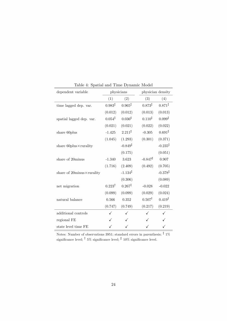
Table 4: Spatial and Time Dynamic Model

dependent variable physicians physician density

(1) (2) (3) (4)

time lagged dep. var. 0.983z 0.965z 0.873z 0.871z

(0.012) (0.012) (0.013) (0.013)

spatial lagged dep. var. 0.054z 0.036] 0.110z 0.099z

(0.021) (0.021) (0.022) (0.022)

share 60plus -1.425 2.211] -0.305 0.691]

(1.045) (1.293) (0.301) (0.371)

share 60plus�rurality -0.849z -0.235z

(0.175) (0.051)

share of 20minus -1.340 3.623 -0.847] 0.907

(1.716) (2.409) (0.492) (0.705)

share of 20minus�rurality -1.134z -0.378z

(0.306) (0.089)

net migration 0.223y 0.267z -0.028 -0.022

(0.099) (0.099) (0.029) (0.024)

natural balance 0.566 0.352 0.507y 0.419y

(0.747) (0.749) (0.217) (0.219)

additional controls X X X Xregional FE X X X Xstate level time FE X X X XNotes: Number of observations 3951; standard errors in parenthesis; z 1%signi�cance level; y 5% signi�cance level; ] 10% signi�cance level.

24

Table 5: Summary Statistics

Mean Std. Dev. Min Max

physicians 271.53 433.10 51 7894

physician density 141.96 47.54 68 391

share 60plus 23.44 2.72 13.8 33.4

share 60plus�rurality 126.24 61.68 18.5 271.8

share of 20minus 21.38 2.32 15 29

share of 20minus�rurality 116.89 57.84 15 239.4

net migration 2.16 7.66 -43.1 57.2

natural balance -1.63 2.66 -10.2 7.1

population size 186160.3 214296.7 35499 3471418

population density 509.49 656.79 40 4024

GDP per capita 22.77 9.32 10.1 85.4

employment rate 48.11 15.29 20.9 139.1

unemployment rate 11.66 5.34 3.0 31.4

share of welfare recipients 28.45 16.41 3.4 138

share of foreigners 6.95 4.85 0.1 28.9

high school leavers 22.22 7.94 0 52.2

no formal education 9.28 2.70 1.4 26

share of new houses 88.80 9.81 29.2 100

new �ats 12.31 7.42 0 69.3

tourist accommodation 36.38 49.71 0.6 581.1

cars per habitants 528.09 51.65 350 959

rurality 5.39 2.52 1 9

Notes: Number of observations 3951.

25

Table 6: Rurality

Type I: Agglomeration Regions

1 Independent Cities with more than 100,000 inhabitants

2 Districts with at least 300 inhabitants per square kilometer

3 Districts with at least 150 inhabitants per square kilometer

4 Districts with less than 150 inhabitants per square kilometer

Type II: Urbanised Regions

5 Independent Cities with more than 100,000 inhabitants

6 Districts with at least 150 inhabitants per square kilometer

7 Districts with less than 150 inhabitants per square kilometer

Type III: Rural Areas

8 Districts with at least 100 inhabitants per square kilometer

9 Districts with less than 100 inhabitants per square kilometer

Notes: The criteria for Type I regions is that they have a concentrated

hinterland. Type III regions are de�ned by a low number of inhabitants

per square kilometer. The remaining regions are merged to Type II areas.

In contrast to the Type III regions they have a higher urbanisation degree,

a rudimental metropolitan centre, and a higher density.

26