demographic aspects of educational planning -...

Demographic aspects of educational planning

Ta Ngoc Ch8u

Unesco : International Institute for Educational Planning

This publication has been financed by the government of the Netherlands through the Fund of the United Nations for Development Planning and Projections (FUNDPAP)

Published in 1969 by the United Nations Educational, Scientific and Cultural Organization Place de Fontenoy, 75 Paris-7c Translated from the French by IIEP Printed by Koninklijke Drukkerij G. J. Thieme, N.V., Nimeguen Cover design by Bruno Pfilffli

0 Unesco 1969 IIEP.66/11.9/A Printed in the Netherlands

Fundamentals of educational planning-9

Included in the series:*

1. What is Educational Planning? P. H. Coombs 1

2. The Relation of Educational Plans to Economic and Social Planning R. Poignant

3. Educational Planning and Human Resource Development F. Harbison

4. Planning and the Educational Administrator C. E. Beeby

5. The Social Context of Educational Planning C. A. Anderson

6. The Costing of Educational Plans J. Vaizey, J. D. Chesswas

7. The Problems of Rural Education V. L. Griffiths

8. Educational Planning: the Adviser’s Role Adam Curle

9. Demographic Aspects of Educational Planning Ta Ngoc Chlu

10. The Analysis of Educational Costs and Expenditure J. Hallak

11. The Professional Identity of the Educational Planner Adam Curle

12. The Conditions for Success in Educational Planning G. C. Ruscoe

* Also published in French. Other titles to appear

Fundamentals of educational planning

The booklets in this series are written primarily for two groups: those engaged in-or preparing for-educational planning and administration, especially in developing countries; and others, less specialized, such as senior government officials and civic leaders, who seek a more general understanding of educational planning and of how it can be of help to over-all national development. They are devised to be of use either for private study or in formal training programmes.

The modern conception of educational planning has attracted specialists from many disciplines. Each of them tends to see planning rather differently. The purpose of some of the booklets is to help these people explain their particular points of view to one another and to the younger men and women who are being trained to replace them some day. But behind this diversity there is a new and growing unity. Specialists and administrators in developing countries are coming to accept certain basic principles and practices that owe something to the separate disciplines but are yet a unique contribution to knowledge by a body of pio- neers who have had to attack together educational problems more urgent and difficult than any the world had ever known. So other booklets in the series represent this common experience, and provide in short compass some of the best available ideas and experience concerning selected aspects of educational planning.

Since readers will vary so widely in their backgrounds, the authors have been given the difficult task of introducing their subjects from the beginning, explaining technical terms that may be commonplace to some but a mystery to others, and yet adhering to scholarly standards and never writing down to their readers, who, except in some particular speciality, are in no sense unsophisticated. This approach has the

Fundamentals of educational planning

advantage that it makes the booklets readily intelligible to the general reader.

Although the series, under the general editorship of C. E. Beeby of the New Zealand Council for Educational Research in Wellington, has been planned on a definite pattern, no attempt has been made to avoid differences, or even contradictions, in the views expressed by the authors. It would be premature, in the Institute’s view, to lay down a neat and tidy official doctrine in this new and rapidly evolving field of knowledge and practice. Thus, while the views are the responsibility of the authors, and may not always be shared by Unesco or the Institute, they are believed to warrant attention in the international market-place of ideas. In short, this seems the appropriate moment to make visible a cross-section of the opinions of authorities whose combined experience covers many disciplines and a high proportion of the countries of the world.

Foreword

All of us who are engaged in educational planning, or in writing about it, face the same embarrassing problem; the field is so vast and varied that, in almost any corner of it, we find ourselves working alongside specialists who, in that particular area, know very much more than we do. This is a source of strength rather than weakness if each is willing to admit his ignorance, but the admitting of ignorance is not always simple, as anyone will testify who has greeted a forgotten acquaintance like a long-lost friend only to be driven a couple of hours later to the indignity of asking him his name. Many of us in planning are in much the same position with the technical terms and concepts of colleagues coming from other disciplines; having used them loosely a dozen times in conference or casual conversation, we hesitate to ask exactly what they mean, and another useful verbal tool, hammered out by experts to express a precise idea, has slipped into the miserable category of blunted, fashionable words.

This makes Dr. Ta Ngoc Chau’s booklet so valuable and timely. The findings of the demographer are the foundation on which most educational plans are built, and those who are responsible for the super- structure cannot afford to be hazy on the meaning of the terms he uses or the true significance of the figures he produces. The crudest error the unskilled planner can make is to ignore, in whole or part, the effects of demographic changes on plans for education, but it is almost as dangerous to take at their face value every set of demographic data that is published. Ta Ngoc Chau sets out to warn us against both extremes. His booklet makes no pretence of being a manual on demography (though a useful list of these will be found at the end of this study) and, in a publication of this length, certain topics,

._..- I l..l--_-. . ..I.. ...-_^-___” ll_l -.- -_. _ ._.-

-_1___11

Foreword

such as theories of population and demographic analysis properly so called, have had to be omitted entirely. But no intelligent layman could read this essay without becoming more acutely aware of the significance of the demographer’s work for educational planning at all levels and of the traps into which the unwary can fall unless they know how the figures have been arrived at. With admirable professional restraint the author deals with demographic techniques only up to the point where they must be understood if one is to know the exact limits within which reliance can be placed on the final results.

For a booklet whose purpose is the clarification of concepts and the orderly presentation of technical processes to the layman the In- stitute was perhaps fortunate in finding an author trained in the French tradition. Ta Ngoc Chau is a Viet-Namese who took his first degree in political science at the Institut d’etudes politiques in Paris, doing one year of the course at Stanford University in the United States. He went on to take his doctorate in economics at the Facultt de droit et des sciences Cconomiques in Paris, and was an assistant at that faculty before he became an associate staff member of IIEP.

The author insists that he is not a professional demographer but an economist who has been led into demography by his interest in educational planning. It is this that gives the booklet its essentially practical character; it is written to be of immediate use to planners and administrators in the field and to those who are preparing themselves for these careers. It is in no way intended to make every planner his own demographer, but rather to help them use the findings-and particularly the projections- of the demographer with the proper blend of confidence and caution. The booklet should be of special value in developing countries, where reliable data are often hard to find and where the assumptions on which demographic projections are based are such as to demand skilled interpretation of the figures by practi- tioners who will build on them the educational plans for a whole country.

C. E. BEEBY General editor of the series

Contents

IIltroduction . . . . . . . .

Part One Population structure and its effects on education . . . .

Section I Censuses and the study of population structure

1 Different types of census . . . . 2 Relative value of demographic data .

a. Errors due to sampling . . . . b. Errors due to the organization of the surveys c. Errors of observation . . . .

Section II Structure of the population by age and sex . . . .

1 Inaccurate age data and methods of adjusting the age pyramid . a. Smoothing the age pyramid . . . . . h. Dividing ten-year age groups into five-year age groups . . c. Dividing five-year age groups into single-year groups . .

2 Age structure of the population and educational development . a. Age structure and teacher requirements . . . . b. Age structure and relative load of educational expenditures c. Age structure and school enrolment rates . . . . d. Age structure of the teachers and its effects on the recruitment

and costs of teaching staff. . . . . . .

Section III Population structure by economic activities and the problems of forecasting manpower requirements . . . . .

1 Active and inactive population . . . . . . a. Definition of active population . . . . . .

I1

12

13 14 15 15 16 16

18 20 22 23 24 25 25 26 29

32

35 35 35

Contents

b. Active population and activity rates by age and sex . . 2 Distribution of the population by sectors of economic activity . 3 Distribution of the population by occupation . . . .

Section IV Geographical distribution of the population and the problem of location of educational institutions. . . . . .

1 Measuring the geographical distribution of a population . . 2 Planning the location of schools . . . . . .

Part Two Population changes and their impact on educational planning .

Section I Natality . . . . . . . . . . 46

1 Methods of measuring natality . . . . . . 46 a. The crude birth-rate. . . . . . . . 46 b. Fertility rates . . . . . . . . . 47

2 Natality trends in selected countries . . . . . 48

Section II Mortality . . . . . . . . . . 52

1 Methods of measuring mortality . . . . . 53 a. Mortality rates by age . . . . . . . 53 b. Life tables . . . . . . . . . 56

2 Mortality trends in selected countries . . . . . 60

Section III Population growth and forecasting school enrolment figures

1 Population growth . . . . . . . a. The natural rate of population growth b. Reproduction rate . . . . . .

2 Preparing population projections . . . . a. Calculation of survivors . . . . . b. Birth projections . . . . . .

3 Forecasting school enrolments . . . . a. On the national scale . . . b. On the local scale . . .

Conclusion . . . . . . . . . . 80

Appendix . . . . . . . . . Dividing five-year age groups into single-year groups: the Sprague multipliers . . . . . . . . . .

36 37 38

40 40 42

45

64 64 64 67 69 70 72 74 75 77

81

Introduction

Demographic analysis can be defined as the study of human groups. One way of approaching the study is to try to explain demographic facts, and to seek the causes behind them. This could be called theoretical demographic analysis. Another way is to be content with a purely descriptive study and end up with a ‘statistical description of populations’. In reality, however, the distinction is not as clear as this; population forecasts cannot be made without a minimum of demographic analysis.

Whichever approach is adopted, there are two possible fields of study which are distinct from each other in objectives and in method. Interest may be centred on the actual current situation of the population. This is what is commonly called a static population study, and what is studied in this case is the state of populations, in other words, their structure or composition. On the other hand, interest may be centred on the trend of the population, which is the dynamic aspect of population analysis. The population trend-also-called ‘movement’ of the population-will depend on a certain number of factors, particularly on such demographic events as births, marriages, and deaths.

For the sake of convenience, I shall respect this traditional distinction by examining in Part One the structure of a population and its effects on educational problems, and in Part Two the population trend or movement and its impact on educational planning.

11

t --

Part One

Population stucture and its effects on education

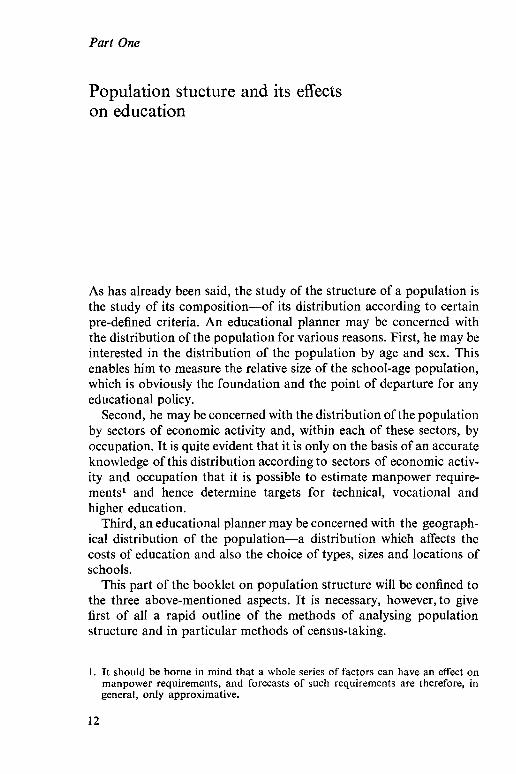
As has already been said, the study of the structure of a population is the study of its composition-of its distribution according to certain pre-defined criteria. An educational planner may be concerned with the distribution of the population for various reasons. First, he may be interested in the distribution of the population by age and sex. This enables him to measure the relative size of the school-age population, which is obviously the foundation and the point of departure for any educational policy.

Second, he may be concerned with the distribution of the population by sectors of economic activity and, within each of these sectors, by occupation. It is quite evident that it is only on the basis of an accurate knowledge of this distribution according to sectors of economic activity and occupation that it is possible to estimate manpower require- mentsl and hence determine targets for technical, vocational and higher education.

Third, an educational planner may be concerned with the geographical distribution of the population-a distribution which affects the costs of education and also the choice of types, sizes and locations of schools.

This part of the booklet on population structure will be confined to the three above-mentioned aspects. It is necessary, however, to give first of all a rapid outline of the methods of analysing population structure and in particular methods of census-taking.

1. It should be borne in mind that a whole series of factors can have an effect on manpower requirements, and forecasts of such requirements are therefore, in general, only approximative.

12

Section I

Censuses and the study of population structure

Governments have always felt the necessity of knowing how many people they govern. Figures of such facts are necessary to determine the volume of recruiting for the armed forces, to distribute the tax load, to make an equitable distribution of land, etc. As the functions of a State increase and its fields of activity widen, a census becomes even more important and the information which needs to be collected becomes constantly greater. Censuses no longer consist in merely counting the population; they now provide the opportunity to obtain a wide variety of information. They have become more and more complex operations, and an increasingly specialized and numerous staff is needed to carry them out. Because of this, the cost of census-taking has greatly increased.

Moreover, owing to the size of the operation, which in principle covers the entire population, and owing to the number and variety of the statistics which have to be compiled, the breakdown and sorting of the census data may take rather a long time. But in population analysis, as in some other fields, statistical data lose some of their value if they are not made known quickly. These data are not intended merely to satisfy a purely scientific interest in the population but are meant, above all, to help us in our planning. This means that we must have the data as promptly as possible. To speed up the process we often restrict the number of questions asked.

There are various possible methods of taking a census, and the choice of method depends to a great extent on the facilities available and the number of personnel which can be used for the operation.

13

Part One

1. Different types of census

The different types of census can be classified according to the precision of the data collected, as follows. 1. A complete census of the population. 2. A survey by sampling. 3. An estimate made in the absence of any real census of the popula-

tion. A complete census of the population is obviously the method which produces the most detailed and the most accurate results. It involves making contact with all the inhabitants of the territory and getting data separately for every one of them. But it can be readily conceived that a total or exhaustive census of the population entails consider- able expense and requires the employment of a large number of persons. That is why a sample census instead of an exhaustive census might have to be used; this is particularly true in many developing countries owing to the shortage of qualified personnel and inadequate financial resources.

Any census is subject to errors of observation, but random sampling introduces in addition a type of error peculiar to itself, derived from the possibility that the sample may not be truly representative of the whole. The fact remains, however, that in census-taking by sampling, the job can be done by a smaller staff which consequently can be better trained and better supervised. Errors of observation can thereby be substantially reduced. In final analysis, the results obtained in a well- conducted sample census may sometimes prove to be better than those obtained in an exhaustive census organized under inadequate conditions.

In the absence of any complete census of the population or of any census by random sampling, a population estimate can be made, based on partial censuses (agricultural, school, etc.) or on entries in special registers, such as tax rolls, voting registers, or lists for rationing services. In any estimating procedures, of course, an error affecting the total population can arise just as well from errors of breakdown as from those due to coefficients or other factors of adjustment which are used in obtaining the total. Such estimates should, therefore, be used with great caution.

Even in countries where the complete census procedure is used, censuses are taken only at comparatively long intervals (ten years, for example). One big problem, therefore, is to get demographic data for

14

Section I

the years between censuses. The surest method is to keep a permanent register of the population. This is done by preparing a card for every individual in the national territory at a given moment, adding new cards for all births or persons entering the territory and removing cards for all deaths or persons leaving. With such a register it is possible to determine at any moment the size and structure of the population. Where there is no such population register, one can attempt toextra- polate the figures on the basis of the trends oberved during the time of the two preceding censuses. An extrapolation of this kind, however, might produce inaccurate results because there would be no assurance that the trends observed in the past would continue into the future. To the extent that fertility and survival rates by age are known, one can also make projections from the data of the last census. I shall have occasion to take up this problem again in Part Two.

I have tried, up to this point, to describe a few methods of taking a census of the population. From this we are already able to see the complexity of the operations of census-taking and the difficulties encountered in obtaining accurate demographic statistics, especially where the necessary facilities are not available, and to see why demographic data are generally not free of errors.

2. Relative value of demographic data

Three types of possible errors can be distinguished: those due to sampling, those due to the organization of the surveys, and those of observation.

a. Errors due to sampling

As we have seen, these errors are linked with the possibility of an unrepresentative character of the sample selected. They will therefore depend on the size of the sample (the larger the sample, the better chance it has to approximate to the actual facts), and on the quality of the sampling, that is, on the skill of the staff in charge of the sampling procedure.

15

Part One

b. Errors due to the organization of the surveys

The organization of demographic surveys is particularly difficult and critical in developing countries. It is evident that the inadequacy of the infrastructure (the scanty development and often poor quality of lines of communication, coupled with the great distances to be travelled in order to make contact with sparse and sometimes mobile populations) and problems of terrain and climate hamper the operation and control of a census. Moreover, it is not easy to recruit sufficient census-taking agents who are trained and capable of carrying out these difficult surveys and who are at the same time willing to work under such conditions. The quality of the data collected in the course of the survey depends, after all, on the competence and the conscientiousness of the census-takers.

c. Errors of observation

It is also in the developing countries that errors of observation are apt to be relatively large. Most demographic data are obtained from statements by individuals; so, when apart of the population is illiterate and when they attach little importance to precise notions of time and date, there is a good chance that some of the statements will be inaccurate.

Faise statements-that is, intentionally untrue statements-must also be reckoned with. These may occur where the people do not understand the exact meaning and purpose of the census questions and suspect that they represent some kind of a government investigation which may have an adverse effect on them in the form of taxes, military service, or other such obligations. There are also cases where super- stition or taboos forbid revealing certain facts of one’s life. It is readily seen, therefore, how important and delicate the work of the census- takers is, for they must instil conhdence in the people, explain to them why the information is being collected, and, in short, win their sincere co-operation.

The many errors which infiltrate into a census-taking operation because of the above-mentioned factors can only be corrected to the extent that the direction of error-whether upward or downward-and the relative size of the errors is known. That is why a control census is sometimes carried out; it is applied to a reduced number of groups or units but it is accomplished with better facilities and a more highly

16

Section I

qualified staff. The comparison of results obtained in the control census with those obtained in the initial census makes it possible to discover the types of errors committed, their upward or downward trend, and their relative size.

Although demographic data will often contain errors, the educational planner must nevertheless use them as his basis for taking certain decisions and for determining certain educational targets. He should therefore inform himself on the methods by which the data were obtained and especially on their degree of accuracy. He must always bear in mind the relative value of such statistics in his work and should allow a certain margin, or room for adjustment, in his plans, so that he can eventually compensate for the effects of errors which have been made in population estimates.

One of the most important items of information gathered in a census is the age of each individual, which makes it possible to determine the age structure of the population.

17

Section II

Structure of the population by age and sex

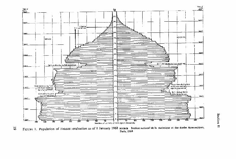
The simplest method of studying the population structure by age and by sex is to construct an ‘age pyramid’. As an example, figure 1 illustrates an age pyramid for the population of France in 1968.

A study of the age structure of the population is very important in demographic analysis because it summarizes, as it were, the demographic past of the nation, and also because, as we shall see in Part Two, it governs to a certain extent the future trend of the population.

The age structure summarizes the demographic past of the nation. The numbers at each age or in each age group depend on: (a) the number of births in the generation or generations from which they have come; (b) the effect of mortality on that generation or those generations; (c) the size of migrations at different times and the ages of the migrants.

Hence, a close examination of a population pyramid is sufficient to reveal the past events which may have affected the population of a country. In the case of the age pyramid of the population of France, the effects of the second world war are clearly marked. A decided decline in the number of births is seen during the years of hostilities, but that decline is more than made up for by the increase of births in the postwar years (1946-1950), an increase which is often referred to as the ‘baby boom’. The baby boom apparently ended in 1951, although the slowing-down of the number of births at that point was extremely slight. The demographic effects of the first world war can be examined in the same way: the same shortage of births during the years of hostilities (19141918) and a similar increase of births in the early postwar years (1920 and 1921). Moreover, an unusually high male death-rate is observed for the generation born between 1880 and 1900,

18

I ‘1‘ i

Gi FIGURE 1. Population of France: evaluation as of 1 January 1968 SOURCE Institut national de la statistique et des Ctudes konomiques,

Paris, 1968

Part One

that is, the men who were eligible for military service during the years of the war.

This is the kind of information that can be obtained by interpreting the irregularities of an age pyramid. But for the conclusions to be true, the irregularities of the pyramid must be real, that is, based on actual facts and not on inaccuracies such as in statements by individuals.

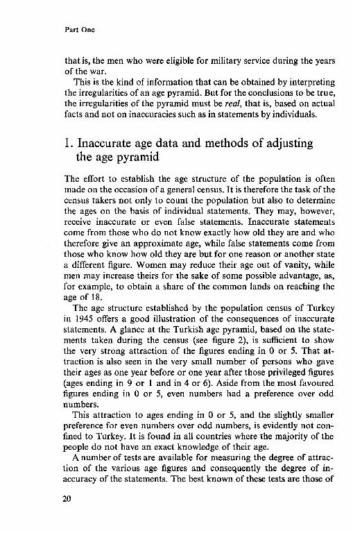
1. Inaccurate age data and methods of adjusting the age pyramid

The effort to establish the age structure of the population is often made on the occasion of a general census. It is therefore the task of the census takers not only to count the population but also to determine the ages on the basis of individual statements. They may, however, receive inaccurate or even false statements. Inaccurate statements come from those who do not know exactly how old they are and who therefore give an approximate age, while false statements come from those who know how old they are but for one reason or another state a different figure. Women may reduce their age out of vanity, while men may increase theirs for the sake of some possible advantage, as, for example, to obtain a share of the common lands on reaching the age of 18.

The age structure established by the population census of Turkey in 1945 offers a good illustration of the consequences of inaccurate statements. A glance at the Turkish age pyramid, based on the statements taken during the census (see figure 2), is sufficient to show the very strong attraction of the figures ending in 0 or 5. That attraction is also seen in the very small number of persons who gave their ages as one year before or one year after those privileged figures (ages ending in 9 or 1 and in 4 or 6). Aside from the most favoured figures ending in 0 or 5, even numbers had a preference over odd numbers.

This attraction to ages ending in 0 or 5, and the slightly smaller preference for even numbers over odd numbers, is evidently not confined to Turkey. It is found in all countries where the majority of the people do not have an exact knowledge of their age.

A number of tests are available for measuring the degree of attraction of the various age figures and consequently the degree of inaccuracy of the statements. The best known of these tests are those of

20

Section 11

FIGURE 2. Population of Turkey in 1945 by sex, age, and five-year age groups according to the census data

SOURCE United Nations, Methodr of Appraisal of Quality of Basic Dam for Popularion Estimates, p. 34. New York, 1955 (Population studies, no. 23, ST/SOA/Series A.)

21

Part One

Whipple, Myers and Bachi. The United Nations Secretariat has also advocated a method of its 0wn.l

An age pyramid of the type shown in figure 2 is of course too in- exact to be utilized directly. Adjustments must therefore be made. Let me say immediately-for there is a tendency to lose sight of the fact- that the main purpose of an adjustment is to get as close as possible to reality. The purpose is not to produce a pyramid which would be more regular, or shall we say more aesthetic, in form, or more in conformity with some ‘model’ age pyramid. Irregularities resulting from the demographic past of the nation must not be effaced under the pretext of making an adjustment. Thus, the irregularities to be observed in the age pyramid of France are explained to a great extent by the events of the past.

a. Smoothing the age pyramid

In so far as the inaccuracy of the statements of age is due to the attraction of the figures ending in 0 or 5, the grouping of ages in con- secutive five-year age groups reduces the inaccuracies, because in each five-year group there is an age ending either in 5 or in 0. That has been done in the age pyramid for Turkey (parts shown in outline without shading).

If irregularities-which are not explained by past events*-still remain after this first adjustment, and if it is suspected that they are due to errors in counting or to inaccurate statements, a method can be applied which consists of linking each age group with the two groups which precede it and the two groups which follow it.

If S, represents the number in the age group considered, S-, and S-, the two preceding age groups, and S, and S, the two following age groups, the adjustment formula is the following:

S’() = ~(-S~,+4S~,+10 so+4 s,-S,)

S’O being of course the adjusted number in the age group considered.

1. Considering the objectives and the size of this booklet, it is not possible to enter into a description of these tests. Interested readers can find a very clear explanation in the manual published by the United Nations: Methods of Appraisal of Quality of Basic Data for Population Estimates, pp. 40-43, op. cit.

2. In the case of Turkey, the small number of children under 5 years of age in comparison with those from 5 to 9, is perhaps explained by the lower birth- rate and the increase of infant mortality during the period of the second world war.

22

Section II

This method of ‘smoothing’ is very convenient and useful when the data are very inaccurate. Its chief drawback, and the reason why one should be careful in using it, arises from the fact that it erases the irregularities without any discrimination. It erases irregularities due to inaccurate statements or breakdown as well as irregularities which really exist. It requires, moreover, a knowledge of the numbers in the two age groups which precede, and the two age groups which follow, the age group concerned. It therefore cannot be applied either to O-4 and 5-9 year age groups or to age groups over 70 years. Age groups over 70 are naturally not of any direct interest to an educational planner, but he should have the most exact knowledge possible of the age groups of O-4 and 5-9 years inclusive. Census figures are in general relatively exact in so far as the 5-9 age group is concerned. Parents are, in fact, able to give a fairly correct estimate of the ages of their children in that group. Incorrect statements are nevertheless sometimes made, as in cases where the parents overstate the age of their children in the hope of getting them into school sooner. On the other hand, experience shows that the counting of the children in the O-4 age group is often incomplete, with the result that the numbers in that group are under- estimated. The figures should therefore be used with care and should be corrected when possible by using the results of the control censuses which may sometimes be made.

b. Dividing ten-year age groups intoJive-year age groups

Population statistics are not only inaccurate; they are sometimes in- sufficiently detailed. It may occur, for example, that only ten-year age groups are available and that data are required concerning five-year age groups. In that case the following formula can be used:

f* = *[fo+Q(f-l-f+l)l

in which f0 is the numerical strength of the ten-year age group concerned, f-, the strength of the preceding ten-year group and f+l the following ten-year group. Then, f, is the first five-year group of the ten-year group concerned, and the second five-year group fb is obtained by subtraction: fb = f,,-fa.

Let us assume that we have the following numerical distribution: O-9 4 500

lo-19 4200 20-29 4050

23

Part One

and that it is desired to divide the lo-19 age group into two five-year groups (10-14 and 15-19).

Application of the above-stated formula gives: f-m-14 = Hfm-1e+Nl-s -f2c41

that is: fill-14 z ~~800+6(4500-4050)1

fis+ = 4200-2 128 = 2072

c. Dividing$ve-year age groups into single-year groups

It may also happen that data for five-year age groups are available and that data are desired concerning single-year age groups. For example, in the planning of primary education, it may be desirable to know not only the numbers of children in the 5-9 and 10-14 age groups but also the actual numbers of children aged 6, 7, 8, 9, etc. In such a case, an interpolation can be effected by using the Sprague multipliers. Details concerning this method are given in the appendix.

The Sprague multipliers are simple to use and undoubtedly constitute a convenient working instrument for the educational planner. It is appropriate to bear in mind, however, that this method is nothing but an interpolation. The results obtained are therefore only approxi- mations, or, to be more precise, they are results which we can consider as being probable. The method should therefore be used only when no data are available other than the figures for the five-year age groups, and especially when there is reason to believe that there has been no great variation in the birth-rate (or, what amounts to the same thing, a variation in the infant mortality rate) in the preceding years. An example of this is a shortage of births due to hostilities or a baby boom of postwar years. It is obvious that such shortages or increases in the birth-rate could have a decisive effect on the numbers of children of certain ages after a corresponding number of years. In that case, if relatively accurate birth statistics which go back far enough are available, and if survival rates are known for different ages, it is undoubtedly preferable to estimate the numbers of children at different ages on the basis of the number of births and of the survival rates. I shall explain the procedure for making such estimates in Part Two.

It is true that, by using methods of adjustment-and I have cited some by way of illustration-and also by making interpolations to

24

Section II

break up the age groups, one can obtain figures that seem to be accurate and detailed. Of course, no method of adjustment, however ingenious, can guarantee getting exact figures from data which are themselves of doubtful accuracy. Although the educational planner should be well aware of the inaccuracies of population statistics, he cannot disregard demographic data. They are the foundation on which his planning is built, and they play a part whenever options are for- mulated or decisions taken. But he must not lose sight of the limits to their accuracy, which call for a measure of flexibility and some freedom of action when questions of policy are being decided.

2. Age structure of the population and educational development

1 have previously shown how a population pyramid can be inter- preted. But a close study of such a pyramid reveals other characteristics which may be very important for the educational planner.

a. Age structure and teacher requirements

The age pyramid for France (figure 1, p. 19) illustrates that there has been a continuous decline in births in France since 1922 (a decline which is clearly shown by a narrowing of the pyramid) which becomes still more pronounced during the second world war. This declining birth-rate undoubtedly results partly from a changed attitude towards having children, but it is also due to other causes, such as the 1914-1918 war which reduced the number of persons born during those years who would have reached the age of procreation some twenty or twenty-five years later.

However, a decided upward change in the birth-rate is observed as from 1945. Not only was there a baby boom in the immediate postwar years, but the increased birth-rate trend has continued. Popula- tion phenomena of this nature can of course have a great effect on education. Thus, in France at the present time (1969) it is, generally speaking, the persons born since 1945 who are in school (either in primary, secondary or higher education) and, as we have seen, the birth- rate since 1945 has been high. The teaching staff, on the contrary, must be recruited from among the generations born before 1945, and these generations were comparatively less numerous. Demographic data alone

25

Part One

thus provide a partial explanation of the relative shortage and difficulty of recruiting teaching staff. This situation will of course rapidly improve in the future, when teaching staff can be recruited from among the greater numbers born since the second world war.

In a more general way, whenever, for one reason or another, there is an increase in the birth-rate (or a decrease in infant mortality), this increase in the number of children results six years later in an increase in the intake of primary school pupils, twelve years later in an increase in secondary school enrolment and eighteen years later in a greater number of university entrants.l This is so obvious that sometimes it is overlooked and preparations for it are not made. In these circumstances, when the extra pupils reach the different stages of education, last-minute improvised arrangements have to be made. Moreover, the problem is often further aggravated by the fact that the arrival of these increased numbers coincides with an increase in the social demand for education. The number of pupils is then increased at one and the same time because the students belong to the years of of higher birth-rate and because there is an increase in the student enrolment rates by age.

b. Age structure and relative load of educational expenditures

Expenditures on education are proportionate to enrolment and consequently depend indirectly on the school-age population, but the financing of education can be considered as a levy on the production of the economically active part of the population. If the school-age population is made up of children from 5 to 14 years of age, inclusive, and the active population is recruited from persons aged 15 to 64, an estimate of the relative load of educational expenditures on the active population is obtained by establishing the proportion of the 5 to lCyear-old population to those of 15 to 64 years of age.

The proportion is far from being the same in the different countries of the world, as is shown in table 1.

What this proportion shows is the youthfulness or the agedness of a population. A population is said to be young when the number of very young people in proportion to the total population is relatively high. When that proportion is low, the population is said to be old.

1. Taking, as is often the case, the official age for admittance to primary school as 6 years and that both the primary schooling and the secondary schooling last six years.

26

Section II

TABLE 1. School-age population and working-age population

(2) Population Age 15-64

(1) Population

Country Age S-14

Nicaragua 1963 462 710 Costa Rica 1963 387 718 Honduras 1961 542 889 Philippines 1960 7 804 825 China (Taiwan) 1963 3 392 241 Mauritius 1963 199900 Togo 1961 406 580 Southern Rhodesia 1962 991700 Syria 1960 1 163 238 Niger 1962 856 268 Sudan 1964 3 651000 Puerto Rico 1960 648 736 Venezuela 1964 2 289 157 Martinique 1961 77 513 Peru 1961 2618558 Panama 1960 262 010 Morocco 1960 2 955 570 Ghana 1960 1699 881 Republic of Korea 1960 6 233 369 India 1961 113937000 Indonesia 1961 23 502 368 Chile 1960 1817 798 New Zealand 1961 529 620 Canada 1961 3935521 Japan 1960 20 222 173 United States of America 1960 35465272 Australia 1961 2 067 505 Uruguay 1963 467 300 France 1962 8 238 302 Italy 1961 8 208 867 Sweden 1960 1 143 670 Fed. Republic of Germany 1961 7 740 800

SOURCE United Nations, Demographic Yearbook, 1964, New York, 1965 ____

749 745 655 259 936 931

13 792 280 6 033 555

360 500 744 480

1820 100 2 132099 1 575 003 6 749 000 1224 199 4 361 544

152314 5236393

526 140 5 981930 3 516 832

13 366055 245 110000 53 249 000 4 134 852 1 407 393

10 655 171 59 939 100

106 977 422 6 436 945 1653 600

29 137 697 33 365537 4949016

36 221018

The youthfulness or agedness of a population is easily seen in its age pyramid. (See figure 3.)

In a country where the birth-rate is very high and where the general death-rate is also very high, the age pyramid has an extremely wide base, but the levels narrow very rapidly owing to the high death-rate. This is type 1.

If the high birth-rate continues together with a declining death-rate,

(l,:(Z 61.7 59.1 57.9 56.6 56.2 55.4 54.6 54.5 54.5 54.4 54.1 53.0 52.4 51.0 50.0 49.8 49.4 48.3 46.6 46.5 44.1 44.0 37.6 36.9 33.7 33.1 32.1 28.3 28.2 24.6 23.1 21.4

27

Part One

I I

1 Form 1

Form 2

Form 4

FIGURE 3. Age pyramids

28

Form 3

Form 5

Section II

(especially declining infant mortality), the base of the pyramid remains wide, and the levels also narrow less rapidly. This is type 2.

If the decline in the death-rate is accompanied by a decline in the birth-rate, the trend is towards type 3. The base is not so wide and the pyramid looks more inflated.

If the birth-rate continues to decrease, the base of the pyramid will become increasingly narrower, as in type 4.

Finally, if the birth-rate, after having decreased, again shows an increasing trend (rejuvenation of the population), it is represented by type 5.

It should be noted that all the pyramids have the same total area. The distinction between them is therefore not the size of the total population. It is the diferent distribution of the population by age which gives different shapes to the pyramids. It is evident that in pyramids of type 1 and 2 the proportion of very young people is high, while it is low in type 4. However, it tends to increase again if the movement is towards type 5. In developing countries, age pyramids of type 1 are frequently found, and still more frequently type 2, while in developed countries the other three forms are predominant.

c. Age structure and school enrolment rates

As we have seen, the age structure enables us to estimate the size of the school-age population. It also enables us to measure accurately the school enrolment rates. Very frequently, in the developing countries, the school enrolment rate is calculated by comparing the total numbers in a level of schooling (primary education for example) with the corresponding age group at the official ages for that level of schooling. This method of calculating usually results in an overestimation of the school enrolment rate; owing to late entry and repetition of courses, many children are older than the official age. Thus the ages of school children only roughly correspond to the official age of their levels of education. Table 2, for example, shows the age distribution of pupils in primary and junior secondary schools in Uganda in 1965. This distribution is shown in figure 4 in the form of an age pyramid.

Although the official age for primary and junior secondary schooling is 6 to 13 inclusive, pupils of 16 and over are occasionally found. Thus, a comparison of the total number of primary and junior secondary school pupils with the 6 to 13-year-old population, will result in an

29

Part One

TABLE 2. Uganda, primary and junior secondary pupils, by age and sex, 1965

Age Girls Boys TOtal

5 and under 6410 7 505 13 915 6 23 029 27 343 50 372 I 24 296 31578 55 874 8 24 806 32 768 57 574

9 23 240 32 466 55 706 10 25 912 41096 67 068 11 20 147 34 497 54 644 12 23 925 48 359 12 284

13 20313 45481 65 794 14 14095 40 778 54 873 15 3931 14 709 18 640 16 and over 1443 10 072 11515

SOURCE Uganda Government, Ministry of Education, Educarion Stofistics 1965, table A 15 -- -

I?

II

I 10

9

s

I I

6

5

50 40 30 20 10 thousands 10 20 25

FIGURE 4. Age pyramid based on data in table 2

30

Section II

overestimation of the proportion of 6 to 13-year-old children who are actually enrolled in school.

Sometimes, instead of comparing the total number of students in a given level of schooling with the number of children in the official age group for that level, the comparison is made between the numbers of pupils in different grades with the numbers of children corresponding to the official age of these grades. This approach provides a more detailed picture, but the disadvantage of the other method exists here as well. What is true for a complete level of education is also true for each grade of that level. A good example of this is shown in table 3 which gives the age distribution of pupils in grade 6 in twenty-five primary schools in Gabon in 1962. (It is to be noted that the official age for students in grade 6 is 11.)

TABLE 3. Age distribution of grade-6 pupils in Gabon, 1962

ABe Boys Girls Total

10 1 1 2 11 5 4 9 12 23 11 34 13 96 38 134 14 115 50 165

15 95 16 108 17 61 18 26 19 8

52 54 21 4

-

147 162 82 30 8

20 9 21 3 22 1 23 1 Total 552

- - - -

235 787

SOURCE J. Proust, ‘Les d&xrditions scolaires au Gabon’, in Efudes ‘Tiers Monde’: Problhes de planification de I’dducation, Paris, Presses universitaires de France, 1964, p. 120

- ~-

For these reasons, in order to obtain an accurate idea of school enrolment in a country, it is necessary to calculate the school enrolment rates by age, that is, the proportion of the children of each age who are actually in school. It is also of value to separate them by sex, since the rates for the two sexes may be different.

As an illustration table 4 shows the school enrolment rates in the Philippines in 1960. The data on the school-age population and the

31

Part One

TABLE 4. School enrolment by age and sex in the Philippines, 1960

Aae

Total Boys

Number Enrolment Total Girls

Number Enrolment population

ww

6 481 7 484 8 434 9 359

10 436 11 298 12 417 13 313

14 301 15 288 16 275 17 268

enrolled percentage population enrolled percentage wm WQ) (ow

15 3.2 448 16 3.7 121 25.0 455 124 27.3 209 48.2 408 210 51.5 227 63.1 343 228 66.4

289 66.3 405 280 69.0 215 72.0 283 209 74.0 278 66.7 379 255 67.2 200 63.9 306 188 61.5

155 51.7 296 140 47.3 122 42.2 277 104 37.5 95 34.5 292 85 29.2 76 28.2 271 62 22.7

SOURCE Census of the Philippines, I960, Population and housing, vol. II Sumnrary report, Manila, 1961

number actually enrolled in schools are shown in pyramid form in figure 5. It will be seen that in the Philippines, as in Turkey, there is a decided preference for giving the children’s ages in even numbers. This applies to children not in school as well as to those actually enrolled. For example, the number of children whose ages were given as 10 or 12 was considerably greater than those said to be 11.

The age pyramid technique can also be used for purposes other than calculating the school-age population. It can be applied, for example, to the teaching staff.

d. Age structure of the teachers and its efects on the recruitment and costs of teaching staff

One of the major causes of the loss of teaching staff is retirement.’ Thus, an accurate knowledge of the age structure of the teaching force is essential in order to prepare for these losses. For example, figure 6 shows

1. This is not always the case. The proportion of those who leave the teaching force long before their retirement can be quite high. In England and Wales, for example, out of 1,000 women enrolled in colleges of education, 900 enter teaching. Only 267, however, remain after eight years. A certain number of these may later return to teaching, but even so the total figure never reaches more than 409. As for men, out of 1,000 enrolled in colleges of education, 673

32

Section II

16

15

14

13

I.?

11

10

9

s

6 i

7

SW 400 300 200 100 thousands 100 200 3co 400

FIGURE 5. Age pyramid based on data in table 4

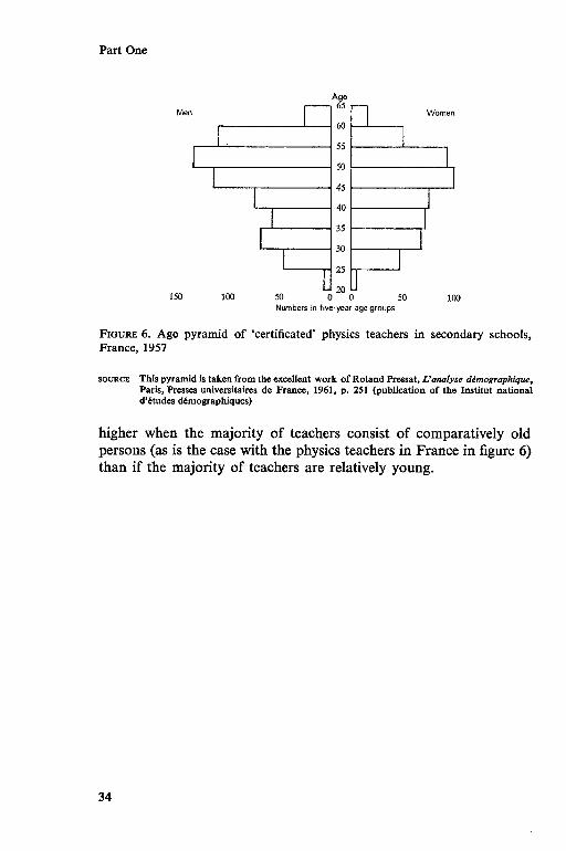
the age pyramid of ‘certificated’ physics teachers in secondary schools in France in 1957. This pyramid clearly shows that the proportion of teachers over 45 is relatively large. Retirement is optional from 60 to 65 and obligatory at 65. It is therefore easy to predict that the number of teachers who will retire during the following fifteen years will be relatively large, thus making it necessary to boost recruitment in order to replace the retiring teachers, as well as to meet the needs of increased enrolments.

Another possible application of the age pyramid to the teaching staff is concerned with salaries. Since teachers’ salaries are geared to levels of seniority, the age structure, or better still the structure by year of seniority of the teaching staff, enables an accurate forecast to be made of the financial effects of changes in the pay scale. It is obvious that the average salary, and consequently the unit costs, are

remain in teachingafter eight years and the number decreases regularly thereafter. (United Kingdom, Department of Education and Science, The Demand for and Supply of Teachers, 1963-1986. Ninth Report of the National Advisory Couticil on the Training and Supply of Teachers, London, HMSO, 1965, p. 84.) However, due to the lack of more detailed data, those teachers who left general education to teach in technical institutes or to teach abroad are considered here to have left the teaching force.

33

Part One

Age 65 6

Women Women

69 69

55 55

50 50

45 45

‘;. ici:B !I. ici:B 40 40

35 35

30 30

25 25

20 20 150 100 100 50 50 0 0 0 0 50 50 100 100

Numbers in five-year age groups 150

Numbers in five-year age groups

FIGURE 6. Age pyramid of ‘certificated’ physics teachers in secondary schools, France, 1957

SOURCE This pyramid is taken from the excellent work of Roland Pressat, L’amlyse dkzographique. Paris, Presses universitaires de. France. 1961, p. 251 (publication of the Institut national d%tudes demograpbiques)

higher when the majority of teachers consist of comparatively old persons (as is the case with the physics teachers in France in figure 6) than if the majority of teachers are relatively young.

34

Section III

Population structure by economic activities and the problems of forecasting manpower requirements

The first problem is to know the percentages of the total population devoted to different economic activities. In other words, it is the problem of distinguishing between the active and the inactive population.

1. Active and inactive population

This apparently simple distinction actually presents a number of difficulties. The problem is to give an exact and unambiguous definition of active population-far from easy if we take into account all the complexities of real situations. By way of illustration, here are some typical difficulties which may be encountered.

It is quite evident that household servants and family helpers should be considered as economically active persons. But what about housewives or other female members of a family who do exactly the same work? Difficulties of a similar nature may arise in connexion with agriculture. In this sector, the activity is essentially seasonal and the work differs in nature and in intensity according to the periods of the year. At peak times (harvesting, for example) many persons are hired, but they are engaged only for periods of intense activity. Should they be listed as economically active persons? Similar questions arise concerning part-time workers, young men doing their military service, etc.

a. Definition of active population

To show the complexity of classifying the active population, the following is the definition proposed by the United Nations. The active

35

Part One

population designates ‘all persons of either sex who provide the human resources for the production of goods and services’.l It includes theoretically the following groups. 1. Civilian employers, employees, own-account workers and unpaid

family workers. 2. Armed forces. 3. Employed and unemployed persons, including those seeking work

for the first time. 4. Persons engaged in part-time economic activities. 5. Domestic servants. The inactive population, on the other hand, consists of persons who do not exercise any economic activity. It includes housewives, students, retired people and children below working age.

However, this very broad definition by the United Nations is not universally accepted, and thus care must be taken when making comparisons between countries. For example, in many countries, people seeking employment for the first time are not included in the economically active population, nor are unpaid family workers, members of the armed forces and part-time workers.

b. Active populations and activity rates by age and sex

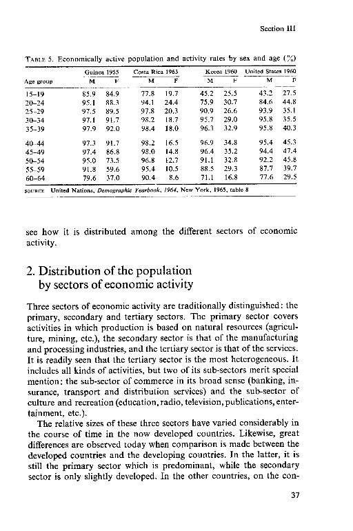
Obviously, the proportion of economically active persons varies according to age and sex. For this reason, it is useful to calculate by sex the percentage of the population in each age group who are counted as being economically active. Table 5, for example, sets out some figures for the economically active population and activity rates by sex and age in four countries.

As the table shows, the activity rates for men aged 20 to 59 are very high and are very nearly the same for all four countries. On the other hand, marked differences are apparent in the 15-19 age group (dependent on length of schooling) and also in the data for women. The rate of economic activity for women is particularly low in Costa Rica but very high in Guinea. These differences may be partially the result of national characteristics, but most of all, they are due to differences in definition of the active population.

Once the active population has been estimated, it is appropriate to

1. United Nations, Principles and Recommendations for National Populafion Censuses, New York, 1958, para. 414 (58.XVII.5).

36

Section III

TABLE 5. Economically active population and activity rates by sex and age (%)

Age group Guinea 1955 Costa Rica 1963 Korea 1960 United States 1960 ---~-- --

M F M F M F M F

15-19 S5.9 84.9 77.8 19.1 45.2 25.5 43.2 21.5 20-24 95.1 88.3 94.1 24.4 75.9 30.7 84.6 44.8 25-29 97.5 89.5 97.8 20.3 90.9 26.6 93.9 35.1 30-34 97.1 91.7 98.2 18.7 95.1 29.0 95.8 35.5 35-39 91.9 92.0 98.4 18.0 96.3 32.9 95.8 40.3

40-44 97.3 91.7 98.2 16.5 96.9 34.8 95.4 45.3 45-49 97.4 86.8 98.0 14.8 96.4 35.2 94.4 41.4 50-54 95.0 73.5 96.8 12.7 91.1 32.8 92.2 45.8 55-59 91.8 59.6 95.4 10.5 88.5 29.3 87.7 39.7 60-64 79.6 37.0 90.4 8.6 71.1 16.8 71.6 29.5

SOURCE United Nations, Demographic Yearbook, 1964, New York, 1965, table 8

see how it is distributed among the different sectors of economic activity.

2. Distribution of the population by sectors of economic activity

Three sectors of economic activity are traditionally distinguished: the primary, secondary and tertiary sectors. The primary sector covers activities in which production is based on natural resources (agriculture, mining, etc.), the secondary sector is that of the manufacturing and processing industries, and the tertiary sector is that of the services. It is readily seen that the tertiary sector is the most heterogeneous. It includes all kinds of activities, but two of its sub-sectors merit special mention: the sub-sector of commerce in its broad sense (banking, in- surance, transport and distribution services) and the sub-sector of culture and recreation (education, radio, television, publications, enter- tainment, etc.).

The relative sizes of these three sectors have varied considerably in the course of time in the now developed countries. Likewise, great differences are observed today when comparison is made between the developed countries and the developing countries. In the latter, it is still the primary sector which is predominant, while the secondary sector is only slightly developed. In the other countries, on the con-

37

Part One

trary, the size of the primary sector has become much smaller in relation to the secondary and tertiary sector. Table 6 illustrates the distribution of the active population by sectors of the economy in selected countries in 1960.

TABLE 6. Distribution of the active population by sectors of the economy, selected countries, 1960 (%)

Primary Secondary Tertiary country sector sector sector

Ghana 59.7 12.4 27.9 Morocco 57.9 10.8 31.2 United Arab Republic 56.9 31.6 11.5 Japan 33.5 29.2 37.2 France 21.4 36.1 42.5 Federal Republic of Germany 13.4 47.7 38.9 United States of America 7.5 34.0 58.5

SOURCE Derived from data in the United Nations Demographic Yearbook, 1964, New York, 1965, p. 240 et seq.

This classification into only three sectors of economic activity is obviously too general to be used for any detailed calculations. In order to make comparisons between countries, the United Nations prepared an international standard classification of all economic activities (ISIC), based upon nine divisions of economic activity.’ However, in addition to this distribution by divisions of activity, the distribution by occupations must also be known in order to forecast manpower requirements.

3. Distribution of the population by occupation

The distribution of the population by occupation does not necessarily correspond to the distribution by sectors of activity. While all farmers will, of course, be listed in the agricultural sector, a mechanic, for example, may work in any of such diversified branches as agriculture, mining, manufacturing industry, electricity supply, and transport.

To make international comparisons easier, the International Labour Office prepared an international standard classification of occupations

1. United Nations, International Standard Industrial ClassiJication of AII Economic Activities, New York, 1958. (Statistical papers, series M., no. 4, rev. 1.)

38

Section III

(ISCO) based upon ten major groups of occupations.1 In order to prepare forecasts of manpower requirements, it is often necessary- as all sectors of economic activity do not develop at the same pace- to make cross-classifications giving, for example, the classification by occupation within each sector. In this way, if the expected increase of production in each sector of activity is known, the manpower requirements for the various occupations or types of employment can be estimated on the basis of this cross-classification. Nevertheless, a difficult problem still remains in linking the job to the qualification, that is, matching the occupation to the type of training received.

In any event, no matter how carefully a forecast of manpower requirements is made, the forecast can only be approximative. One should therefore proceed with extreme care in planning the future enrolments in technical and higher educati0n.l

This type of information on the structure of the population by economic activity is of importance to educational planners. But there is another aspect of the population structure which may also be of great interest to them, namely, the geographical distribution of the population.

1. International Labour Office, International Standard Classification of Occupations, Geneva, 1958.

2. The following Dublications are recommended for study on these Droblems: F. Harbison:-Educational Planning and Human Resourie Developnht, Paris, Unesco/IIEP, 1967. (Fundamentals of educational planning, 3.); H. S. Pames, Forecasting Educational Needs for Economic and Social Development, Paris, OECD, 1962.

39

Section IV

Geographical distribution of the population and the problem of location of educational institutions

The distribution of the population in a country is, of course, far from uniform; some areas are densely populated, others much less so.

When there is no co-ordinated policy (such as a regional development plan), the development of individual areas may be very unequal and the difference between areas may continue to increase. Thus, the population of already densely inhabited areas may continue to grow, while scarcely populated areas become depopulated. In other words, the geographical distribution of a population is never static, and this poses problems for educational planners.

1. Measuring the geographical distribution of a population

A study of the population density of different areas constitutes a preliminary assessment of the geographical distribution of a population, but, in order for a survey of this kind to have meaning and usefulness, it must focus on the smallest geographical or administrative units, as an average density figure is necessarily of less significance. But when the only available population data are based on random sampling in a limited number of administrative units, and when the results are later extrapolated to the whole of the territory, the figures arrived at make it impossible to know the population of many administrative units. In these conditions the estimate of population density is, to say the least, extremely vague. A large town or city in an area automatically raises the density rate of the administrative unit and thereby falsifies the data for the rural areas contained in that unit.

40

Section IV

For this reason, the population of urban centres is sometimes excluded from the estimates.

Another way of estimating the geographical distribution of the population is to classify the administrative units according to the number of their inhabitants. But here again there is a drawback because the over-all size of the population does not provide any indication of the local characteristics of the society (whether it is concentrated or dispersed). Such data on an area are an important factor in planning the location of educational premises.

By way of illustration, table 7 shows the distribution of villages in Morocco according to size of population. It will be noted that the great majority of Moroccan villages have a population of less than 500, a feature which presents problems for the development of education in rural areas.

TABLE 7. Distribution of villages in Morocco according to size of population

Population Number of villages Percentage of total

Less than 300 From 300 to 499 From 500 to 999 From 1000 to 2 000 Over 2 000

SOURCE Unpublished document

20 662 68.6 5 580 18.5 3 132 10.3

601 1.9 136 0.7

Moreover, what is important for educational planners is not only the current distribution of population, but also its future trend. It is therefore necessary to study internal migrations. It must be admitted that as a general rule very little is known about these population shifts inside a national territory. While the periodical censuses make it possible to determine the rate of growth of different areas (urban centres in particular), the percentage of that growth which is due to natural increase and the percentage which is due to internal migrations are not known, and still less is known about the age and origin of the migrants.l

1. I shall take up this problem again in Part Two of this booklet in studying population movements. See, in particular, pages 77 and 78.

41

Part One

2. Planning the location of schools

Two considerations which may sometimes be contradictory must be taken into account in locating schools: the size of population and the catchment areas of the school.

In so far as the size of population is concerned, one thing is evident. There must be a certain minimum number of pupils living in an area in order to justify the building or installation of a school. This problem is complicated in the case of secondary schools with their greater number of both compulsory and optional subjects.

It is also important that the area served should not be too large, so that the pupils can easily reach the school from their homes. The acceptable limits of that area obviously depend on the ages of the children, the facilities offered, (e.g., the existence of a school lunch room), the means of transport available, and whether or not the climate is severe. Of course, in an area of dense population, the problem does not arise. There is always a sufficient population so that the area served by the school need not be too large. But the situation is different in areas of more dispersed population and especially in rural areas.

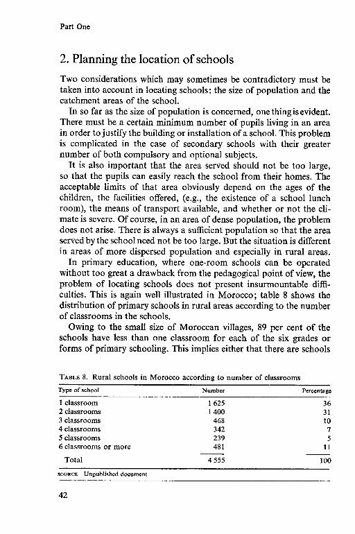
In primary education, where one-room schools can be operated without too great a drawback from the pedagogical point of view, the problem of locating schools does not present insurmountable difficulties. This is again well illustrated in Morocco; table 8 shows the distribution of primary schools in rural areas according to the number of classrooms in the schools.

Owing to the small size of Moroccan villages, 89 per cent of the schools have less than one classroom for each of the six grades or forms of primary schooling. This implies either that there are schools

TABLE 8. Rural schools in Morocco according to number of classrooms

Type of school Number Percentage

1 classroom 1625 36 2 classrooms 1400 31 3 classrooms 468 10 4 classrooms 342 7 5 classrooms 239 5 6 classrooms or more 481 11

Total 4 555 100

SOURCE Unpublished document

42

Section IV

which provide only partial schooling or that several grades share the same room with the same teacher. It should be noted, however, that the pupil/teacher ratio is lower in the rural schools than in the urban areas (31.7: 1 as compared with 44: 1).

At the secondary level of education, because of the optional courses offered and the subjects to be taught, the number of students must be much greater to justify the creation of a school. Depending on the size of the local population, its age distribution and the proportion of children attending school, the catchment area for the secondary school may be very large. When this area becomes too large, the provision of a school bus pick-up system or the accommodation for boarding students may be necessary. But all this will obviously increase the cost-and it is on the basis of the comparative costs that the final choice of one solution or another can be made.

In any event, it must be understood that the location of schools cannot be based on purely theoretical considerations. Many factors have to be taken into account (population trend, means of transport, other economic and social factors) and all these factors may vary from one area to another. It is therefore at the local level that people know them best, and that is why, as far as possible, the local authorities should be fully involved in the location of schools.

Another problem arises from the differences in the proportion of children attending schools in different areas. In selecting school sites, should areas where participation rates are particularly low be favoured at the risk of obtaining small numbers of pupils or should more schools simply be provided where the population density makes it easily justifiable to build more schools? It is not easy to answer this question which involves a matter of principle. Should the total number of students be increased to the maximum, or, on the contrary, should equal opportunities be provided for all boys and girls regardless of where they live? The problem is further complicated by the fact that the unit costs in different areas are not the same (due, in part, to lower pupil/teacher ratios and the necessity of paying salary bonuses to encourage teachers to take less desirable posts). Following the same line of thought, it must be noted that as the school enrolment rate increases, the problems of establishing schools are multiplied and the objective of compulsory schooling implies the creation of schools in the most out-of-the-way places and on the least favourable sites, with all the consequences which all that can have on the cost.

Planning the location of schools is further complicated in multi-

43

Part One

ethnical and multi-lingual countries by the need to take such special local characteristics into account.

So far, I have discussed the structure of a population in its different aspects and tried to show the effects which that structure may have on the planning of education. But educational planners cannot be content with knowing the present situation; they must also have an accurate picture of the problems to be encountered in the future. In particular, they must know what the trend of that population will be in future years. That is the subject to be tackled in the following pages, by studying population changes and their impact on educational planning.

44

Part Two

Population changes and their impact on educational planning

The study of population changes must take into account the trend of any increase (or, rarely, decrease) in the population over a period of time. Obviously, the two main factors which affect this trend are natality and mortality. The combination of these two factors, plus migration, determine the changes in size of a population. These are the factors which will now be discussed.

45

Section I

Natal&y

In this section, I shall first discuss the ways of measuring natality and then look at some of the trends in natality in selected countries.

1. Methods of measuring natality

Two main rates are used to estimate natality; either the crude birth- rate or the fertility rate.

a. The crude birth-rate

This, the simplest rate, is obtained by comparing the number of live births during a year with the average population for that year. The average population for a year can be considered either as the population figure for 1 July of that year or as the average of the population figures for the beginning and the end of the year.

It is to be noted that, as a rule, the birth-rate is given per thousand. This is also done for other demographic rates.

Although the crude birth-rate has the advantage of being a simple rate, easily obtained from general data, it nevertheless has certain disadvantages. One of these disadvantages is that it gives the ratio of live births to the total population, whereas, in fact, only a part of the female population is of child-bearing age. Consequently, the crude birth-rate may vary according to the age structure of the population, in particular the percentage of women of child-bearing age in relation to the total population. This rate, therefore, cannot be used to make comparisons between countries, because the age structures may be so

46

Section I

different. This is why demographers prefer to use the fertility rate rather than the crude birth-rate.

b. Fertility rates

In discussing fertility,% the first thing to say is that the term itself implies a linkage between the number of births and the number of women of child-bearing age. A distinction can be made, however, between the general fertility rate and the fertility rate by age.

1. The general fertility rate. This rate is the ratio of live births to the number of women of child-bearing age (generally considered to be women of 15 to 49). As in the case of the crude birth-rate, this rate is expressed per thousand. If the total number of births is related to the total number of women aged 15 to 49 years (married and un- married), we obtain a general fertility rate. If, on the other hand, we take into account only legitimate births and married women we obtain a legitimate fertility rate.

One of the drawbacks of the general fertility rate is that it does not give an accurate idea of fertility. It is a known fact that fertility varies with age and is particularly strong in women between 20 and 30. Therefore the general fertility rate of the population may be higher or lower according to the proportion of women aged 20 to 30. For this reason planners prefer to calculate the fertility rate by age.

2. FertiZity rate by age. Fertility rates can of course be calculated for each year of age (by finding, for example, the ratio of the number of live births by 20-year-old mothers to the total number of women aged 20). But, in general, fertility rates are given by age groups (ages 15-19, 20-24, 25-29, etc.). As shown above, general fertility rates by age and legitimate fertility rates by age can be calculated separately.

Where there is no voluntary birth control, the fertility rate by age provides a relatively accurate measurement of the number of births. When these rates are known, it is possible to forecast the number of

1. A distinction is sometimes made in demographic analysis between ‘fertility’ and ‘fecundity’, fecundity referring to the biological capacity for having children (potential fertility) and the word fertility being used to refer to actual births (actual fertility). The two terms mean the same thing when there is no intentional limitation of births, or birth control, but otherwise they are different in meaning, as a ‘fecund’ couple may in fact remain voluntarily childless and therefore lack ‘fertility’.

47

Part Two

future births with some degree of accuracy. But where birth control is practised, the use of these rates may prove to be very difficult. When the size of the family is voluntarily restricted and when the births are voluntarily spaced, the age of the women is no longer the only factor affecting fertility. Other factors come into the picture, such as age at marriage, length of time married, the number of children preceding a given birth. Under such conditions, it is easily seen that the fertility rate by age becomes less significant. Nevertheless, in spite of such shortcomings, as long as they are used with precaution, the fertility rates by age are still the best way of forecasting future births. (This point will be taken up again when studying methods of making population projections.)

Having thus analysed the different ways of measuring natality, I shall now turn to natality trends in selected countries.

2. Natality trends in selected countries

It is sufficient to glance at figure 7, showing the number of births in Sweden from 1900 to 1965, to see how much natality can vary in a country over a period of time.

With the notable exception of 1920, the number of births in Sweden

thousands

150 c

1 I I I I I I I I I I I I I I

1900 1910 1920 1930 1940 1350 1960 1970

FIGURE 7. Trend of births in Sweden (1900-1965) SOURCE OECD, Education Policy and Planning in Sweden, Paris, Directorate for Scientific Affairs,

1966, p. 19 (DASIEIPj66.37.)

48

Section I

steadily dropped from 1900 to 1935. It then increased, the increase being particularly large between 1940 and 1945. It then dropped again; that decline can be linked with the smaller number of people born after 1920 arriving at the age of reproduction in the late 1940s and 1950s. In 1960 the direction of the curve changed again.

In the face of such great variations, it is easy to see the danger of trying to extrapolate the number of future births from past trends. Nevertheless, the number of future births has great significance for educational planners. It is evident that the number of births in future years will determine the number of pupils and students in the various levels of education. Although at the present time in most of the developing countries educational planning is mainly concerned with increases in numbers of pupils and students, in other countries-after a period of declining natality-educational planning may be involved in planning for a decline in numbers of pupils and students.

It must be realized, however, that a decline in the birth-rate is not the only cause of a declining number of school pupils. As will be seen later, internal migration of the population may cause the number of inhabitants in rural areas to change very decidedly. In such cases, the result may be a drop in the number of pupils and under-utilization of rural schools, while at the same time, new schools must be built in urban areas to accommodate the children of the new influx of families. In this way, planning for an increased number of pupils may take place simultaneously with planning for decreased numbers in the same country.

The decline in natality which was observed in Sweden at the end of the nineteenth and the beginning of the twentieth century was a general phenomenon in all countries of western Europe. While the crude birth-rate had been about 40 per thousand in the eighteenth century in most of these countries, it then dropped to 18 per thousand, the lowest rate being reached in the period between the two world wars.

But when there is a systematic policy of birth control and that policy is effectively applied, the decline in the birth-rate may be even more rapid. Table 9 shows that Japan’s crude birth-rate dropped in ten years from 30 per thousand to 18 per thousand, that is, to a level comparable to that of western European countries.

Other countries which have judged their population growth to be too rapid have also tried to apply a policy of birth control. The results obtained have often been rather disappointing, however, either because of the resistance of the population or because of the relatively

49

Part Two

TABLE 9. Trend of the crude birth-rate in Japan (O/&

Yet%3 Rates YCCUS Rates

1945-49 30.2 1962 17.1 1950-54 23.7 1963 17.3 1955-59 1 a.2 1964 17.7 1960 17.2 1965 18.6 1961 16.9 SOURCB United Nations, Demographic Yearbook, 1965, New York, 1966, p. 293

complicated nature of the methods used. For these two reasons, it seems that the general level of education of the population-and the example of Japan proves the point-is a decisive factor for the success of such a policy.

But while natality may vary with time, it varies still more greatly when comparisons are made between countries. By way of illustration, table 10 gives the crude birth-rates for selected countries of the world in 1964.

TABLE 10. Crude birth-rate in selected countries in 1964 (“/,,)

Country Rate Country Rate

Developed countries United States of America Canada United Kingdom Fed. Rep. of Germany France Japan

Africa Gambia RBunion Madagascar Mauritius

21.2 23.8 18.7 18.2 18.1 17.7

44.9 43.3 42.4 38.1

Latin America El Salvador Honduras Mexico Venezuela Nicaragua

Asia Burma Malaysia China (Taiwan)

46.8 *46.3 45.2

*43.4 41.8

39.7 *39.4 34.5

SOURCE United Nations, Demographic yearbook, 1964, New York, 1965, pp. 527-536 * 1963

As can be seen, the crude birth-rate of developing countries aver- ages between 40 and 45 per thousand, which is about double the rate of most of the developed countries. But as the crude birth-rate depends on the age structure of the population, it is not a really accurate way of making comparisons between countries. It is thus preferable to compare the fertility rates by age, as shown in table 11.

50

Section I

TABLE 11. Fertility rates by age for selected developed and developing countries (“1.0) Country 15-19 20-24 25-29 30-34 35-39 4044 45-49

Sweden United

Kingdom Fed. Rep. of

Germany France Portugal Peru China

(Taiwan) Panama Mauritius

1962 40 133 142 84 38 10 0.6

1960 34 165 172 101 46 14 0.8

1963 30 145 185 103 50 17 0.8 1962 23 167 177 107 53 19 1.1 1963 27 139 178 137 95 45 3.3 1961 78 231 245 201 153 74 18

1963 43 252 337 231 139 61 9.8 1962 151 310 288 199 129 41 7.2 1963 104 309 288 245 161 67 6.8

SOURCE Calculated from data in United Nations, Demographic Yearbook, 1964, New York, 1965 pp. 130-155 and pp. 537-543

-

The first point to notice is that the fertility rates at all ages are higher in the developing countries than in the developed countries, which was to be expected. But what is also to be noted is that the difference is comparatively low for the 20-24 and 25-29 age groups but is greater for the other age groups and especially for those between 40 and 49 years of age. This shows the difference between people who practise voluntary limitation of births and those who do not, or at least not to a significant extent. Where birth control is practised, as soon as the family has reached the preferred size, an effort is made to avoid any further births, and this preferred size may be reached while the mother is still comparatively young. Where no birth control is practised, potential fertility (fecundity) and actual fertility are the same, and the trend of actual fertility by age is linked mostly to biological factors. In this case, as I have shown, it is possible to make fairly accurate forecasts of future births from the fertility rates by age.

Having analysed natality, I shall turn to the second factor which can affect population change, namely, mortality.

51

Section II

Mortality

Two types of mortality are usually distinguished, according to the causes of death: endogenous mortality and exogenous mortality.

Endogenous mortality means death occurring from a cause which is to some extent inherent in the individual. Thus, when a child is born with deformities and dies because of these deformities, its death can be placed in this category. Also in this category are deaths due to old age or diseases which accompany old age such as vascular lesions and cancer.

Exogenous mortality, on the other hand, is linked with other causes, such as accidents, contagious diseases, and alimentary deficiencies.

Although this may appear to be a very clear-cut distinction, it is not all that clear when real situations are examined, because the causes of death may be unknown or not declared, or because the causes of death may be multiple. Nevertheless, the distinction is very useful, An interesting fact is that, although the progress of hygiene and of medical care, on the one hand, and the raising of the standard of living, on the other hand, are capable of reducing exogenous mortality to a marked extent, they have very little effect on endogenous mortality. Medical progress indeed can prevent certain premature deaths but cannot prolong life beyond a certain limit. Hence, when there is a decline in mortality, it affects the younger generations rather than the older ones. The result is that a decline in the mortality rate has the effect of creating a younger population (an increase in the younger section of the population in comparison with the older part).

As in the case of natality, we shall examine successively the ways of measuring mortality, and then the trend of mortality in selected countries.

52

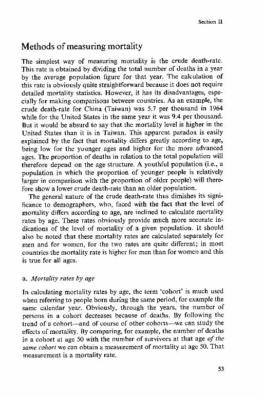
Section II

Methods of measuring mortality

The simplest way of measuring mortality is the crude death-rate. This rate is obtained by dividing the total number of deaths in a year by the average population figure for that year. The calculation of this rate is obviously quite straightforward because it does not require detailed mortality statistics. However, it has its disadvantages, especially for making comparisons between countries. As an example, the crude death-rate for China (Taiwan) was 5.7 per thousand in 1964 while for the United States in the same year it was 9.4 per thousand. But it would be absurd to say that the mortality level is higher in the United States than it is in Taiwan. This apparent paradox is easily explained by the fact that mortality differs greatly according to age, being low for the younger ages and higher for the more advanced ages. The proportion of deaths in relation to the total population will therefore depend on the age structure. A youthful population (i.e., a population in which the proportion of younger people is relatively larger in comparison with the proportion of older people) will therefore show a lower crude death-rate than an older population.

The general nature of the crude death-rate thus dimishes its significance to demographers, who, faced with the fact that the level of mortality differs according to age, are inclined to calculate mortality rates by age. These rates obviously provide much more accurate indications of the level of mortality of a given population. It should also be noted that these mortality rates are calculated separately for men and for women, for the two rates are quite different; in most countries the mortality rate is higher for men than for women and this is true for ail ages.

a. Mortality rates by age

In calculating mortality rates by age, the term ‘cohort’ is much used when referring to people born during the same period, for example the same calendar year. Obviously, through the years, the number of persons in a cohort decreases because of deaths. By following the trend of a cohort-and of course of other cohorts-we can study the effects of mortality. By comparing, for example, the number of deaths in a cohort at age 50 with the number of survivors at that age of the same cohort we can obtain a measurement of mortality at age 50. That measurement is a mortality rate.

53

-- --

Part Two

The calculation of mortality rates needs detailed statistical data, including statistics covering the number of deaths at a given age and the number of survivors at the same age for the same cohort. In many cases, however, these detailed statistics are not available. It is therefore necessary to calculate the death-rates at different ages, and these rates in turn give the proportion of deaths of persons of each respective age during the calendar year compared with the average total number of individuals of that age during that same year.

The death-rates certainly give valuable information concerning the mortality characteristics of a population. They do not, however, enable us to make more detailed calculations, and in particular to establish mortality tables, to which we shall refer later. For that reason, an effort has been made to convert from death rates to mortality rates.

1. Conversion from death-rates to mortality rates: the Reed-Mere11 method. By examining the populations of different states of the United States in 1910, 1920 and 1930, for which both the death-rates and the mortality rates were available, Reed and Mere11 endeavoured to find connecting links between these respective va1ues.l It is impossible here to go into all the details of their methods of calculation. But the results of the Reed-Mere11 work have been published in the form of tables giving the equivalent mortality rate for all likely values of death- rates of the four-year, five-year and ten-year age groups.

Obviously, the fact that Reed and Mere11 based themselves on the statistics of the United States in establishing the relationships between death-rates and mortality rates limits somewhat the scope of their work, as it is undoubtedly true that the mortality structure and rates by age for the developing countries do not always correspond exactly to those which have been observed in the United States during the period covered.

In spite of this reservation, it must be said that the Reed-Mere11 tables are a very convenient working tool and that they make it possible to convert rapidly from death-rates to mortality rates when there are no other available means of doing so.

2. Comparison of levels of mortality between countries. We have already noted that the crude death-rate is a very imperfect way of comparing mortality levels between countries. Mortality rates by age are much

1. L. J. Reed and M. Merell, ‘A short method for constructing an abridged life table’, The American Jourmd of Hygiene, Sept. 1939, vol. 30, no. 2, pp. 33-62.

54

Section II

more accurate for this purpose but they have the disadvantage, however, of being too detailed and analytical. So, when there is a need to make such comparisons, an age-standardized death-rate, based upon the detailed data, is used. This rate may be calculated either by applying different mortality rates to a standard population (the ‘direct standardization method’) or by applying a standard set of rates to different populations (the ‘indirect standardization method’). Either method will result in an estimate of the number of deaths expected in one population, based upon information from another population. This number of expected deaths can then be used to calculate the standardized death-rate.

For example, if a comparison is needed between mortality in the United States and that in Taiwan, either method may be used to arrive at the standardized death-rate.

The direct method consists of first asking how many deaths would be expected in the United States if it had the same age structure as Tai- wan. In this way, a standardized rate which eliminates differences due to population age structure is obtained.

For the indirect method, the death-rates by age for Taiwan are applied to the population of the United States. Then, by dividing the real number of deaths in the United States by the number of deaths which would have occurred if the United States had the same death- rate by age as Taiwan, a standardized rate is obtained which enables the mortality of the two countries to be compared.

3. Infant mortality. Special attention should be given in mortality studies to infant mortality, because the mortality rate for very young children is very high. Moreover, the infant mortality level is of much interest to educational planners because the number of children for whom schooling must be provided in the future depends on that level. Infant mortality is measured by the mortality rate at age 0, that is, the ratio of deaths from birth to 1 year of age to the total number of live births. Still-births can be distinguished from infant mortality, and the distinction can be carried even further to includeperinatal mortality.

We have already spoken of the differences between endogenous and exogenous mortality and have pointed out that endogenous mortality in the case of infants relates to those who are born alive but considered as being doomed to a very short existence in the present state of medical knowledge. Perinatal mortality is therefore obtained by adding endogenous mortality to still-births,

55

Part Two

Finally, we have two overlapping concepts: Perinatal mortality = still-births-tendogenous mortality Infant mortality = endogenous mortality+exogenous mortality

While the concepts of perinatal mortality and infant mortality are theoretically very accurate, their measurement is often imperfect, especially in developing countries. A very large proportion of infant deaths (and of births) are often not registered. The difference between true still-born and not really still-born (children who are live born but who die before their birth is declared) is a source of great difficulty even in countries where registration procedures are well organized.

b. Life tables

Life tables show the number of survivors at different ages of a group of individuals of the same cohort or generation. Let us assume for example that it has been possible to follow up a group of 10,000 persons since their birth 100 years ago to the present date. Of this group, 1,600 died before reaching the age of 1 year, 300 others before reaching the age of 2 years, 200 others before reaching the age of 3, and so forth. From these figures the number of survivors at different ages can be derived.

10000 births 8400 survivors at 1 year 8 100 survivors at 2 years 7900 survivors at 3 years, etc.

A table of this kind has an undoubted historical value because it traces what happens to a generation over a period of time. It is not, however, of any current practical utility because it is linked to the mortality characteristics of the past. Thus, the number of survivors at age 1, indicated in the above figures, resulted from the infant mortality of a century ago. For this reason, instead of constructing life tables based on a real cohort, tables derived from current situations are constructed-based on a theoretical cohort. The principle of construction of these tables is simple; starting with a theoretical cohort of 10,000 individuals, current mortality conditions (i.e., current mortality rates by age) are applied to that cohort.

For example, mortality rates may be assumed as follows:

56

Section II

Age Mortality rates (“/,,) 0 70 1 18 2 12 3 8

If a cohort of 10,000 is now used, it is immediately evident that the number of deaths at less than 1 year is:

10000x70 loo0

=700

and that the survivors at the age of 1 are lO,OOO-700 = 9,300 Of these 9,300, a certain number die before reaching the age of 2,

a number which is found by applying the mortality coefficient at age 1: 9300 x 18 ~-- = 167

1000

Therefore, the number of survivors at age 2 is 9,300- 167 = 9,133. Continuing these calculations, the following table is obtained:

Age Survivors 0 10000 1 9300 2 9133 3 9024 4 8952

In this way, by knowing the mortality rates at different ages, it is easy to construct a life table. However, as I have previously pointed out, the computation of the mortality rate presupposes the availability of accurate and detailed statistical data. In most of the developing countries, these statistics are often fragmentary and their accuracy is doubtful, making the construction of life tables very difficult. Yet, we shall see that such tables are an indispensable way of establishing future population projections.

In the absence of a life table, provided that at least fragmentary data concerning mortality are available, it is possible to resort to the model life tables which have been prepared by the demographic services of the United Nations.

I. Model life tables. The construction of these tables rests upon a comparatively simple observation. In studying existing life tables, it

57

Part Two

was observed that there is a certain relationship between the mortality rates for different ages. In other words, if the mortality rate at age 35 of a population has a certain value, the mortality rate of that same population at age 45 does not have just any value but, on the contrary, a value which is linked, to a certain extent, to the the first rate.

So, on the basis of the data contained in 158 national life tables covering the period 1900-1950, the demographic services of the United Nations worked out model life tables’ giving the number of survivors of each sex at different ages according to various levels of mortality.

It is not possible to go into detail here concerning the methods by which these tables were worked out.2 We shall simply note that at the beginning, forty model tables were prepared corresponding to infant mortality levels from 200/,, to 3300/,,. Then, with these forty tables twenty-four others, corresponding to life expectations at birth ranging from twenty years to 73.9 years, were interpolated. (We shall have occasion to return to this concept of life expectation at birth, which constitutes one of the component indicators of the different levels of mortality.)

These tables, of course, give only average indications obtainedfrom data relative to human groups in different periods of time and subject to diversified economic and social conditions. Therefore, the application of one of these tables to a particular population involves a certain possibility of error or inaccuracy. It is nevertheless convenient to refer to these model tables when only fragmentary mortality data are available and when there is no other way of establishing a mortality table. By choosing among the model tables the one which corresponds best to the fragmentary mortality statistics which are actually available, data are obtained which, although only approximative, have at least the advantage of being complete and which therefore make it possible to establish population projections.

2. Life expectation. We have already referred to the concept of life expectation and it is now appropriate to clarify this concept further. Life expectation can be defined as the average number of years which individuals of different ages will live. For a population, for example,

1. These tables are given in: United Nations, Methods for Population Projections by Sex and Age, New York, 1956 (Population studies no. 25, ST/SOA/Series A.)

2. For further details, see: United Nations, Age and Sex Patterns of Mortality. Model Life-tables for Under-developed Countries, New York, 1955 (Population studies no. 22, ST/SOA/Series A.)

58

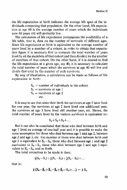
Section II

the life expectation at birth indicates the average life span of the individuals composing that population. On the other hand, life expectation at age 60 is the average number of years which the individuals now 60 years old will probably live.

The calculation of life expectation presupposes the availability of a life table, that is, data on the number of survivals of different ages. Since life expectation at birth is equivalent to the average number of years lived by a member of a cohort, in order to obtain that expectation figure it is necessary first to compute the total number of years lived by all the members of that cohort and then divide it by the number of members of that cohort. On the other hand, if it is desired to find the life expectation at a given age, say 40, it is necessary to calculate the total number of years which the survivors at age 40 will live and divide that total by the number of such survivors.

By way of illustration, a calculation can be made as follows of life expectation at birth :

So = number of individuals in the cohort S, = survivors at age 1 S, = survivors at age 2

etc.

It is easy to see that since their birth the survivors at age 1 have lived for one year, the survivors at age 2 have lived one additional year, the survivors at age 3 have lived still another year, etc. Hence, the total number of years lived by the various survivors is equivalent to:

s,+s,+s,+...

But it can also be considered that those who died between birth and age 1 lived an average of one-half year and it is possible to make the same assumption for those who died between age 1 and age 2, between age 2 and age 3, etc. The number of those who died between birth and age 1 is equivalent to So-S, those who died between age 1 and age 2 equivalent to S,--S,, those who died between age 2 and age 3 equivalent to Ss--Sz, and so forth.

The total correction to be made is then:

~~~o--s,~+~~~,-s2~+3~s2-s2)+...

that is:

B (So-$I+$,-$2+$2-s,+...) = 4 so

59

-- ..- ._.. ____l.I_ --

Part Two

The total number of years lived by the entire cohort is then

g s,+s,+s,+s,+...

and the average numbers of years lived by a member of that cohort, that is, the life expectation of that cohort at birth, is equivalent to:

e 0

= ~s,t&+&+s,+... so

s,+s2+s,+ ... =;+- s 0

The same procedure can of course be used to calculate life expectation at other ages.

Such are the principal ways of measuring mortality. I shall now turn to mortality trends in selected countries.

2. Mortality trends in selected countries

In the countries of western Europe, mortality has declined since the beginning of the nineteenth century. The crude death-rate which was about 300/,, in 1800, is now about 10°/oo. That decline has been gradual and is explained by scientific progress and the improvement of medical and social facilities, as well as by the higher standard of living and the higher cultural level of the people.

In the developing countries, the decline of the death-rate has been much more rapid, as is shown in table 12. It should be noted, however, that this mortality decline is different from that of western European countries in that it is not actually the consequence of an increase in the standard of living, but results instead from recent medical dis- coveries which have made it possible to fight in a very effective way- and at a relatively low cost-against diseases which were taking a heavy toll of human life (cholera, smallpox, the bubonic plague, malaria, etc.).

At the present time, therefore, the crude death-rate in the developing countries is similar to the rates in developed countries; in some cases it is even lower. But as we have seen earlier, the crude death-rate is a very imperfect way of comparing mortality levels between countries. The very low crude death-rate in developing countries is explainable

60

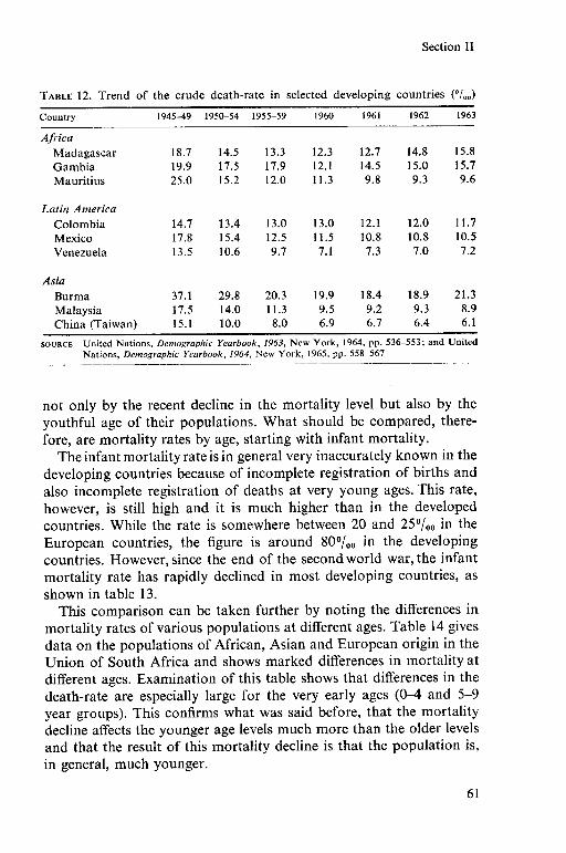
Section II

TABLE 12. Trend of the crude death-rate in selected developing countries (“/,,,)

Countrv 1945-49 1950-54 1955-59 1960 1961 1962 1963

AJiiiCU

Madagascar 18.7 14.5 Gambia 19.9 17.5 Mauritius 25.0 15.2

13.3 12.3 12.7 14.8 15.8 17.9 12.1 14.5 15.0 15.7 12.0 11.3 9.8 9.3 9.6

Latin Americn Colombia 14.7 13.4 Mexico 17.8 15.4 Venezuela 13.5 10.6

13.0 13.0 12.1 12.0 11.7 12.5 11.5 10.8 10.8 10.5 9.7 7.1 7.3 7.0 7.2

Asia Burma Malaysia China (Taiwan)

37.1 29.8 20.3 19.9 18.4 18.9 21.3 17.5 14.0 11.3 9.5 9.2 9.3 8.9 15.1 10.0 8.0 6.9 6.7 6.4 6.1

SOURCE United Nations, Demographic Yearbook, 1963, New York, 1964, pp. 536-553; and United Nations, Demographic Yearbook, 1964, New York, 1965, pp. 558-567

not only by the recent decline in the mortality level but also by the youthful age of their populations. What should be compared, therefore, are mortality rates by age, starting with infant mortality.

The infant mortality rate is in general very inaccurately known in the developing countries because of incomplete registration of births and also incomplete registration of deaths at very young ages. This rate, however, is still high and it is much higher than in the developed countries. While the rate is somewhere between 20 and 25°/00 in the European countries, the figure is around 800/ao in the developing countries. However, since the end of the second world war, the infant mortality rate has rapidly declined in most developing countries, as shown in table 13.

This comparison can be taken further by noting the differences in mortality rates of various populations at different ages. Table 14 gives data on the populations of African, Asian and European origin in the Union of South Africa and shows marked differences in mortality at different ages. Examination of this table shows that differences in the death-rate are especially large for the very early ages (O-4 and 5-9 year groups). This confirms what was said before, that the mortality decline affects the younger age levels much more than the older levels and that the result of this mortality decline is that the population is, in general, much younger.

61

Part Two

TABLE 13. Trend in infant mortality rates in selected developing countries (“/..)

Country 194549 1950-54 1955-59 1960 1961 1962 1963

AJrica Madagascar Gambia Mauritius

132.5 91.9 73.9 69.1 70.6 . . . . . . 114.7 104.9 87.4 66.9 64.6 68.1 68.1 142.8 83.1 67.7 69.5 62.0 60.1 59.3

Latin America Colombia Mexico Venezuela

141.8 113.3 100.9 99.8 89.6 89.6 88.2 104.5 91.8 77.7 74.2 70.2 69.9 67.7 97.5 75.0 64.1 53.9 52.9 47.0 47.9

Asia Burma 303.9 240.3 156.4 148.6

34 139.3 . . .

Singapore 100.4 81.8 56.8 41.5 36.9 33.0 Hong Kong 98.7 69.4 42.3 34.3 32.1 31.0 27.9

SOURCE United Nations, Demographic Yearbook, 1966, New York, 1967, pp. 282 et seq.

TABLE 14. Mortality rates by age of the populations of African, Asian and European origin in the Union of South Africa, 1961 (“/3

Age African Asian Europenn groups Male Female Male Female Male Female

o-4 50.5 5-9 1.7

lo-14 1.1 15-19 2.2 20-24 3.8

25-29 5.0 30-34 6.4 35-39 8.0 40-44 10.7 4549 15.2

50-54 22.5 55-59 26.2 60-64 42.4 65-69 54.6 70+ 107.5

All age groups 16.7

46.0 18.8 1.6 1.0 1.2 1.0 1.7 1.7 2.5 1.8

3.1 2.4 4.6 3.1 6.8 3.7 6.6 6.5 9.1 14.2

14.0 18.7 16.2 26.6 34.6 37.4 40.8 64.2 94.0 135.6

14.2 8.6

14.0 7.8 6.1 1.5 0.7 0.5 0.6 0.6 0.4 1.3 1.3 0.4 1.5 2.6 0.8

2.3 2.1 1.2 2.7 2.8 1.4 3.9 3.5 1.9 5.7 5.6 3.2 9.4 8.0 4.3

13.7 13.1 7.3 20.0 20.6 10.8 37.6 30.7 17.0 75.4 46.3 25.2

125.6 105.6 76.7

6.1 9.9 7.3 SOURCE Calculated from data in United Nations, Demographic Yearbook, 1964, New York, 1965,

tables S and 21

62

Section II

TABLE 15. Expectation of life at different ages in selected countries

India El Salvador Portugal Sweden (195160) (1951-61) (1959-62) (1962)

M F M F M F M F

0 41.89 40.55 44.71 47.39 60.73 66.35 71.32 1 48.42 46.02 51.77 54.13 65.77 70.92 71.64 5 48.72 47.01 51.95 53.94 63.94 69.13 67.88

10 45.21 43.78 49.05 50.88 59.33 64.48 63.05

20 36.99 35.63 42.00 43.59 49.88 54.85 53.40 30 29.03 27.86 34.72 36.08 40.72 45.40 43.94 40 22.07 22.37 27.99 29.14 31.81 36.12 34.50 50 16.45 17.46 21.99 22.90 23.33 27.17 25.45

60 11.77 12.98 16.38 17.07 15.71 18.56 17.25 70 8.07 9.28 11.00 11.53 9.46 11.13 10.55 80 5.13 6.02 6.34 6.65 5.07 5.85 5.72

75.39 75.43 71.62 66.76

56.96 47.21 37.59 28.29

19.55 11.84 6.20

SOURCE United Nations, Demographic Yearbook, 1964, New York, 1965, pp. 620-624

Finally, we can also compare mortality levels on the basis of life expectation at different ages. Table 15, for example, shows life expectations for selected countries. Here again, it is seen that the difference is especially large at the younger ages. On the other hand, at age 80 the life expectation is practically the same for each country. It can also be seen that, with the notable exception of India, life expectation is always higher for women than for men. Another point is that life expectation at age 1 is higher than life expectation at birth, because of infant mortality. The difference is slight, however, in the case of Sweden.

63

Section III

Population growth and forecasting school enrolment figures

Population growth is of special interest to educational planners because of its effect on the school-age population and the future enrolment figures in educational institutions at all levels. In this section, therefore, I shall give much attention to methods of making population projections and forecasting future school enrolments.

1. Population growth

Obviously, it is the joint action of natality and mortality which determines the growth of a population. It is true that international migrations also play a part, but the characteristics of these migrations are peculiar to each country and to each specific situation. Migrational movements are therefore usually set apart; in the total growth of a population the natural growth, which takes into consideration only natality and mortality, is analysed independently.

a. The natural rate of population growth

Since the natural growth is equivalent to the difference between births and deaths, it is sufficient to calculate the difference between the crude birth-rate and the crude death-rate in order to have a measurement of the population growth. This is the crude natural rate of population growth. Table 16 shows the trend of these rates in selected countries during the period 1945-1964.

What is immediately noted in this table is that the rate of natural population growth has increased in most of the developing countries

64

TABLE 16. Crude birth-rates, death-rates and natural growth rates for certain countries, 1945-1964 (“/,)

country 1945-49 1950-54 1955-59 1960 1961 1962 1963 1964

United Kingdom Birth-rate 18.3 15.9 16.4 17.5 17.9 18.3 18.4 18.7 Death-rate 11.6 11.7 11.6 11.5 12.0 11.9 12.2 11.3 Natural growth 6.1 4.2 4.8 6.0 5.9 6.4 6.2 7.4

Japan Birth-rate 30.1 23.7 18.2 17.2 16.9 17.1 17.3 Death-rate 16.8 9.4 7.8 7.6 7.4 7.5 7.0 Natural growth 13.3 14.3 10.4 9.6 9.5 9.6 10.3

Madagascar Birth-rate 24.0 31.9 34.9 32.8 34.8 40.0 41.8 Death-rate 18.7 14.5 13.3 12.3 12.7 14.8 15.8 Natural growth 5.3 17.4 21.6 20.5 22.1 25.2 26.0

Gambia Birth-rate Death-rate

Colombia

Natural growth

Birth-rate Death-rate Natural growth

33.6 37.3 44.4 44.0 43.2 47.9 46.7 19.9 17.5 17.9 12.1 14.5 15.0 15.7 13.7 19.8 26.5 31.9 28.7 32.9 31.0

17.7 6.9

10.8

42.4 16.5 25.9

44.9 13.2 31.7

33.1 37.4 42.4 42.4 43.4 44.1 47.6 14.7 13.4 13.0 13.0 12.1 12.0 11.7 19.0 24.0 29.4 29.4 31.3 32.1 35.9

Venezuela Birth-rate 38.5 44.1 47.1 45.9 45.3 43.4 43.4 Death-rate 13.5 10.6 9.7 7.1 7.3 7.0 7.2 Natural growth 25.0 34.1 31.4 38.8 38.0 36.4 36.2

China (Taiwan) Birth-rate 40.2 45.9 42.8 39.5 38.3 37.4 36.3 Death-rate 15.1 10.0 8.0 6.9 6.7 6.4 6.1 Natural growth 25.1 35.9 34.8 32.6 31.6 31.0 30.2

. . .

. . . . . .

..,

. . .

. . .

34.5 5.8

28.8 if SOURCE United Nations, Demographic Yearbook, 1963, New York, 1964, tables 19 and 23; and United Nations, Demographic Yearbook, 1964,

c New

York, 1965,

tables 16 and 20 Ei

2

Part Two

and that it can reach a very high level. In Colombia and Venezuela, for example, it is over 35°/00. If that rate is continued in the future, the population of those countries will double every twenty years, which means, considering the exponential growth, that their population will theoretically be thirty-two times greater in 100 years! This gives an idea of what is meant by ‘population explosion’ and of the necessity for certain countries to resort to birth control.

This increase in the rate of natural growth is due first of all to the rapid decline in the crude death-rate. This is a general phenomenon in all the developing countries, as we have already pointed out. It is to be noted, however, that the death-rate is still relatively high in countries such as Gambia and Madagascar. On the other hand, it is at a very low level in other countries, such as Venezuela and Taiwan. In other words, mortality may decline further in the African countries and those countries may have in a near future a demographic situation like that in the Latin American and Asian countries.

But while mortality has declined in all of the countries, the birth-rate tends to increase in some of them, and it is this combined action of decrease in mortality and increase in natality which has caused the ‘explosive’ increase of the population in countries such as Colombia and Venezuela.

That is what distinguishes the population situation of the western European countries at the end of the nineteenth century from the present situation in the developing countries. As we have already pointed out, the mortality decline has been very gradual in western Europe and although it preceded the birth-rate decline, the latter caught up with it, so that the mortality decline accompanied by the declining birth-rate did not bring about a too rapid increase of the population. It should also be noted that the ageing of the population (due to the declining birth-rate) prevented the mortality from dropping to very low levels.

In developing countries, on the contrary, the mortality decline has been very rapid, while the birth-rate has held firm or has even slightly increased. Therefore, the result has been a very rapid increase of the population.

It is, of course, very hazardous to try to discover trends when only crude rates are available and especially when one is not quite sure of the accuracy of these rates. In some countries, the increased birth- rate may result simply from better registration of births! It appears, nevertheless, that in a country such as Taiwan, the birth-rate, after

66

Section III

having increased and reached a high level, is beginning gradually to decline. In Japan, that decline is still more rapid and more percep- tible.

A striking feature of table 16 is that where there is no voluntary restriction of birth, the crude birth-rate may reach the very high level of 48°/,,0 (as in the case of Colombia). On the other hand, the death- rate in youthful populations may easily decline to the neighbourhood of 6O/,, (as in Taiwan). The margin that such figures leave for population growth is therefore very large.

It should be noted, however, that the crude rate of natural growth resulting from the crude rates of natality and mortality has the same disadvantages as these two latter rates in that it does not take into consideration the age structure, which may be very different between countries and even in the same country from one period of time to another. For this reason, the concept of ‘reproduction’ may be sub- stituted for the concept of population growth. The basic idea here is to find out to what extent one generation can replace the one from which it has issued. That leads, therefore, to the quantitative comparison of this generation with the one which preceded it.

b. Reproduction rate

If we follow a generation from its birth up to the time when it has completed the procreation of all its descendants, and if we compare the number of these descendants with the number of persons in the generation itself, we obtain a measurement of the ‘replacement’ of one generation by another. This is the principle on which the calculation of the reproduction rate is based.

In general, however, instead of comparing the total number of descendants with the total number in the generation from which they have issued, the number of female births is compared with the number of women in the generation.’ The reproduction rate is therefore equal to the average number of female babies given birth to by women of the generation being considered.

But, of course, we must take into account not only the actual fertility but also the mortality of the women. A certain number of women

1. It should be noted that, in general, more boys are born than girls and that the relative male birth-rate is about 1.05. In other words, out of every 1,000 births

there are approximately 512 boys and 488 girls

67

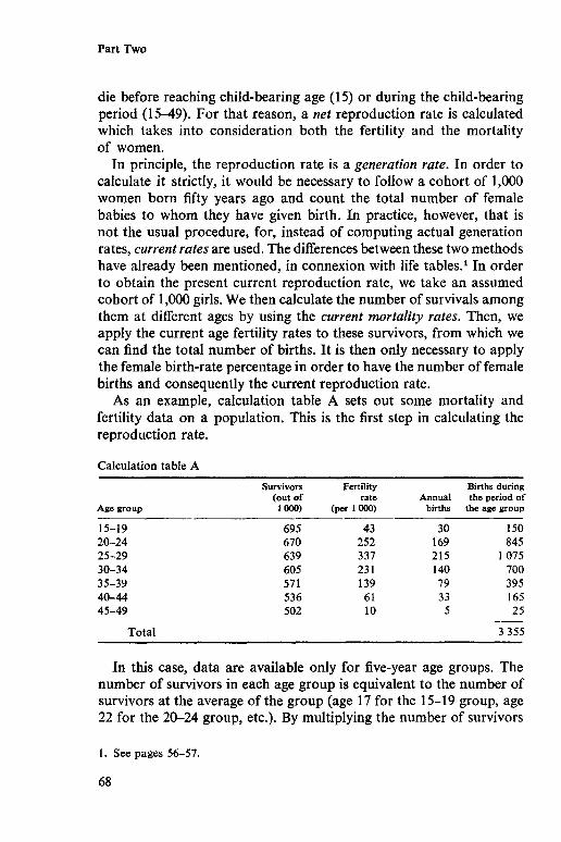
Part Two

die before reaching child-bearing age (15) or during the child-bearing period (15-49). For that reason, a net reproduction rate is calculated which takes into consideration both the fertility and the mortality of women.

In principle, the reproduction rate is a generation rate. In order to calculate it strictly, it would be necessary to follow a cohort of 1,000 women born fifty years ago and count the total number of female babies to whom they have given birth. In practice, however, that is not the usual procedure, for, instead of computing actual generation rates, current rates are used. The differences between these two methods have already been mentioned, in connexion with life tables.’ In order to obtain the present current reproduction rate, we take an assumed cohort of 1,000 girls. We then calculate the number of survivals among them at different ages by using the current mortality rates. Then, we apply the current age fertility rates to these survivors, from which we can find the total number of births. It is then only necessary to apply the female birth-rate percentage in order to have the number of female births and consequently the current reproduction rate.

As an example, calculation table A sets out some mortality and fertility data on a population. This is the first step in calculating the reproduction rate.

Calculation table A

Age WJUP

Survivors Fertility (out of rate

1OW (Per 1 @Jo)

Births during AllIUXll the period of

births the age group

15-19 695 43 30 150 20-24 670 252 169 845 25-29 639 337 215 1075 30-34 605 231 140 700 35-39 571 139 79 395 40-44 536 61 33 165 45-49 502 10 5 25

Total 3355

In this case, data are available only for five-year age groups. The number of survivors in each age group is equivalent to the number of survivors at the average of the group (age 17 for the 15-19 group, age 22 for the 20-24 group, etc.). By multiplying the number of survivors

1. See pages 56-57.

68

Section III

by the fertility rate, the annual number of births is obtained. But as each woman spends five years in each age group, these births must be multiplied by 5. Adding up the births we have a total of 3,355. As an average of 488 females are born in every 1,000 births1 the number of female births is thus 3,355 x 0.488 = 1,637 and net reproduction rate is 1.637. Since the net reproduction rate is higher than 1, it can be concluded that the generation which follows is more numerous than the one which precedes and that the trend of the population is to increase.

In studying the future trend of a population, the net reproduction rate is undoubtedly better than the crude rate of natural growth, which does not express anything other than the current balance between births and deaths. In a period of declining birth-rate, this decline may well be masked by a declining death-rate with the result that the birth/death balance remains positive. But the births may decline to such a level that the generations no longer replace themselves. The population becomes older (increase in the proportion of old people) and after a certain time, it decreases (decrease in total numbers).

The net reproduction rate owes its popularity precisely to the fact that it was the means of showing the danger of depopulation of western Europe in spite of a births-to-deaths balance on the positive side. It is well to note, however, that the reproduction rate, however ingenious it may be, is a current rate and is fully significant only when the demographic conditions are stable. It should be used with caution in the event of any rapid change in conditions.

However, educational planners do not need to know with precision whether or not a generation is able to replace the preceding generation. But they must be able to forecast what the trend of the school-age population will be during the coming years. As we shall see, such a forecast can be made on a relatively certain basis.

2. Preparing population projections

There are two main reasons for making population projections. The first is a purely scientific reason, which leads one to try, for

example, to answer the question of what would be the trend and struc-

1. See page 67, note 1.

69

Part Two

ture of a population if such and such demographic conditions were present. In this way, an attempt can be made, for example, to discover the consequences on the population of a gradual decline in infant mortality during the next twenty years. Projections of this kind are sometimes called conditional projections. They express what would occur if such and such a condition were fulfilled. They evidently do not seek to determine what the actual situation in the future will be, and, in that sense, such forecasts can never be mistaken! Nevertheless, they can be very useful and highly instructive to the extent that they provide a means of discovering indirect consequences of certain possible population changes.

The second concern is of much greater practical usefulness. In this case, a genuine attempt is made to forecast the future population trend. Starting with the current situation, particularly the present structure of the population by sex and age and the present level of mortality and fertility, the basic aim is to project these characteristics into the future. This leads to the estimation of projective rates. Using these projective rates, it is possible to calculate the number of survivors and then complete the picture by making a forecast or projection of births.

a. Calculation of survivors

The calculation of survivors is one of the safest factors in population projection. This calculation deals with cohorts which are already born; the only assumptions which have to be made concern mortality. Now, if the death-rate at the earliest ages (O-4 years) is excluded, the death-rate in the young ages (5-30 years) is low and the risk of error is not very high. For that reason, short-term school enrolment forecasts and active population projections are relatively accurate.

In so far as mortality is concerned, differences have been shown between the mortality rate and the death-rate. But it is evident that instead of considering the number of deaths, the number of survivors can be taken and this enables a calculation to be made, for example, of the proportion of individuals of the same cohort, at a given age who are still living one year later. This gives us what is known as a survival rate.

If out of 420,000 children of a given cohort 2,100 die before reaching the age of 1, the survival rate between ages 0 and 1 is equivalent to:

70

Section III

420000-2 100 420000

= 0.995

However, instead of the survival rate at a given age, we can compute the survival rate for an age group. We can determine, for example, the proportion of children of the O-4 year group who, five years later, will constitute the 5-9 year group.

On the basis of the present survival rates and the probable mortality trend in the near future, we can estimate the projective survival rates. As the mortality level is not the same for men and for women, we must compute these rates separately for each sex.

In this connexion, the model life tables which have been established by the demographic services of the United Nations can again be of some use. These tables offer the advantage of describing the different mortality levels (corresponding to increasingly higher life expectations at birth). The corresponding survival rates are annexed to these tables. Hence, if no other means are available for estimating the projected survival rates and if a certain decline in mortality is nevertheless expected, the survival rates corresponding to a slightly lower mortality level can be used as projective rates. But that, of course, is only a preliminary rough estimate.

When the projective rates have been determined, it is sufficient to apply them to the present population figures for the different ages or the different age groups in order to build the age structure of the future years.

Let us assume, for example, that the age structure of the male population as of 1 January 1965 and the projective survival rates are those given in calculation table B. On the basis of these data, we can easily estimate the male population age structure for 1970.This table gives data for a five-year projection, but, provided the necessary projective rates are available, projections can be established for more distant dates.

However, in a five-year projection based only on a survivor calculation, there is no figure for the O-4 year age group (these children not yet being born). By the same token, in a ten-year projection both the O-4 and the 5-9 age groups will be missing, and so on. For this reason, it is necessary to make birth projections in order to complete the table.

71

Part Two

Calculation table B

kzegroup 1965 Survival rate 1970

04 512300 --, 0.900 - 5-9 452 100 0.969 !-+ 461070

IO-14 377 400 0.970 438 085 15-19 333 000 0.957 366 078 20-24 296 000 0.948 318 681

25-29 259 000 0.944 280 608 30-34 229 000 0.937 244 496 35-39 222 000 0.926 214 573 40-44 199 800 0.908 205 572 4549 170 200 0.885 181418

50-54 118400 0.854 150 627 55-59 103 600 0.811 101114 60-64 74 000 0.751 84 020 65-69 51800 -+ 0.666 - 55 574 70 et + 51800 + 0.520 !+ 61435

b. Birth projections

While the calculation of survivors is made on the basis of the present structure of the population, by sex and by mortality level, birth projections are established on the basis of the age structure of the female section of the population (in particular those of child-bearing age) and the fertility level.

It should be noted, however, that while the mortality rates at the younger ages are low (which reduces the possibility of numerical errors in estimating survivors), the fertility rates, on the contrary, are not low and moreover have a direct effect on the number of births. Thus the birth projections do not give as accurate results as the survivor calculations.’ That is especially true when there is a sudden and un- expected variation in fertility.

In making birth projections, we must begin by calculating projective fertility rates. This can be done by taking the current fertility data and drawing up assumptions as to the trend in the future.

1. Let us look at table B which illustrates this point. The survival rate of the 5-9 age group is assumed to be 0.969. Consequently, the mortality rate of the same age group is 0.031. Let us suppose that that mortality rate has been under- estimated by 10 per cent. This means that the real rate is 0.034 and that the total

72

Section III

The next step is to estimate the number of women in different cohorts. Let us assume, for example, that the projective fertility rates by age and the numbers of women of different cohorts are as shown in calculation table C.

Calculation table C

Years of birth Numbers NUdX3-S Projective fertility of female cohorts at l/1/65 at l/1/70 rates, 1965-69 (“I..)

1950-54 400 800 387 173 145 194549 370000 352 980 700 1940-44 340 400 321338 1055 1935-39 318 200 298 790 895

1930-34 296 000 276 464 680 1925-29 266 400 247 485 415 1920-24 222 000 204 240 155 1915-19 170 500 159 132 25

The cohort of women born between 1945 and 1949 (i.e., those who were in the 15-19 age group as of 1 January 1965) may first be considered. On that date, they number 370,000. However, owing to deaths, their number will be reduced to 352,980 as of 1 January 1970. The average number of these women during the period is therefore

370000+352980 - 2 = 361490

The table shows, moreover, that the fertility rate of this cohort is 7000/,,. The result is that the number of births which can be expected for this cohort during the period is

361490 x 700 1000

= 253043

The same procedure can be followed for the other cohorts: calculation table D shows the result.

number of deaths of the 5-9 age group between 1965 and 1970 is 15,371 instead of 14,015. Therefore, the number of survivors is 436,729 instead of 438,085 and the relative error made in the survivor calculation is

438.085-436.729 438,085

= -$$jg i.e., less 0.1 y0

In other words, a 10 per cent error id the estimation of the mortality rate leads only to an error of less than 0.1 per cent in the survivor calculation.

Conversely, it is clear that an error of 10 per cent in the fertility rate will lead to an error of 10 per cent in the projection of the number of births.

73

Part Two

Calculation table D

Years of birth of female cohorts

Numbers at l/1/65

Average Projective numbers fertility Numbers of

Numbers during the rates, births at l/1/70 period 1965-69 (“/..) forecast

1950-54 1945-49 1940-44 1935-39

1930-34 1925-29 1920-24 1915-19

Total 1271 114

400 800 387 173 370 000 352 980 340 400 321 338 318 200 298 790

296 000 276 464 266 400 247 485 222 000 204 240 170 500 159 132

393 986 361490 330 869 308 495

276 232 266 942 213 120 164 816

145 57 128 700 253 043

1055 349 067 895 276 103

680 187 838 415 110781 155 33 034 25 4120

Now that the total birth figures have been projected, the respective numbers of boys and of girls must be worked out. Assuming that the male/female ratio is 105: 100, the number of boys will be 650,810 and the number of girls 620,304. However, a certain number of these children will die before 1 January 1970, so that in order to obtain the number in the O-4 age group as of 1 January 1970, the preceding figures should be multiplied by the corresponding survival rates. On the basis of the population projections thus established, a forecast of school enrolments can be made.

3. Forecasting school enrolments

Two different stages can be distinguished in the forecasting of future school enrolments. The purpose of such a forecast may be to estimate the total educational costs and to plan the necessary means of finding finance. The figures with which one is concerned in this case are the over-all figures, and this is referred to as the forecasting of enrolment figures on the national scale.

But when it is a question of implementing an educational plan, it is necessary to know also how these school enrolments are distributed in the different areas throughout the country. This involves forecasting on the local scale.

74

Section III

a. On the national scale

The first thing to do here, obviously, is to estimate the school-age population. Population projections showing the future age structure of the population enable this to be easily done. As an example, figure 8 illustrates the case of Sweden. On the basis of births recorded and births forecast, an effort was made to estimate the numbers of the school-age population for compulsory schooling (age 7-15), upper secondary education (age 16-19) and post-secondary education (age 20-24).

Three assumptions have been made concerning fertility, which explains the presence of three birth estimate curves. For the other estimates, however, only an average assumption was taken. (Solid lines in the charts indicate actual figures and dotted lines indicate projected figures.)

It is of course necessary to allow for international migrations. But, as we have already stated, the characteristics of such migrations are peculiar to each country and each particular situation should be analysed. It should be noted, however, that, in general, such migrant movements have very little effect on the school-age population, except perhaps at the post-secondary level. Conversely, they may have a much greater effect on the economically active population.

During the age of compulsory schooling, the forecasting of school enrolment figures does not present any particular difficulties. The school-enrolled population in a country with an effective system of compulsory education is approximately equivalent to the school-age population. But at the other levels the enrolment rates must be in- serted.

These rates can be said to depend on two main factors: on the one hand, the social demand (that is the desire expressed by pupils and their parents) and, on the other hand, the policy established by the government. As a matter of fact, things are not quite so simple in reality. Governments, even the most authoritarian, are obliged to take social demand into account in making their policy. Inversely, there is no government, however liberal it may be, which does not seek to influence that social demand. Thus, in many countries an effort is being made to emphasize and encourage technical education or in- struction in scientific subjects. It is, therefore, finally the combined action of the two factors (social demand and governmental policy) which determines the level of educational enrolment rates.

75

Part Two

150 t

140

130

120

110

100 90

‘i-i’ 11 I I I I I I I I I I I I I I j

1900 1910 1920 1930 1940 1950 1960 1970 1980 Actual and estimated numbers of births

II I I I I I I 1

1950 60 70 80 Age group 7-15

500 \ \ 400

-- r,

300 k

600

500

400

I’ I I I I ’ 1 I II I I I I I I 1

1950 60 70 80 1950 60 70 80 Age group 16-19 Age group 20-24’

FIGURE 8. Trend of the school-age population in Sweden

SOURCE OECD, Educational Policy and Planning in Sweden, Paris, 1966, op. cit.

76

Section I11

Where the effort is made above all to satisfy social demand, the trend of that demand in the future must be estimated. The study of past trends may be quite revealing; on the basis of such rates, the probable level of that rate in the future can be worked 0ut.l

However, if the development of education is considered as a priority task, in other words, if an effort is to be made to facilitate its development to the greatest possible extent (anticipating and encouraging to some extent social demand), the school-enrolment rates then become targets to be achieved. For example, it might be decided to raise the enrolment rate gradually in order to reach general compulsory education within twenty years. Obviously, it will be necessary to bear in mind the financial implications of such targets and avoid allowing the development of education to exceed the financial possibilities of the country.

If the future school-age population is known (thanks to the population projections) and if, as well, it is possible to work out the enrolment rates at different levels, it is a relatively simple step to prepare a forecast of the number of students. But, as stated earlier, in order to implement an educational plan it is not sufficient to forecast only the over-all numbers for a country; it is also essential to try to find how these numbers will be distributed throughout the country. So, after making forecasts on a national scale, it is necessary to make similar forecasts on the local scale.

b. On the local scale

Here, a whole series of problems arise. First of all, the enrolment rates may vary considerably from one area to another. As was pointed out in the section on the location of schools, it is a matter for the government authorities to decide whether the existing differences between the regions should be reduced or whether, on the contrary, education should be developed in the areas where there is the heaviest demand. This is a problem which is complicated by the fact that the financial implications of one decision may be quite different from those of an alternative decision.

Internal migrations must also be taken into account. While international migrations generally have little effect on the school-age

1. In recent years social demand for education has, in general, been increasing very rapidly and the forecasts of numbers of students have turned out to be on the low side in many countries.

77

Part Two

population, internal migratory movements, which are sometimes quite large, may affect it greatly. Increases in the populations of towns and cities are explained at least as much by internal population movements as by the natural growth of the population. Unfortunately, these internal migrations are usually not very well plotted, and in most cases, no accurate data are available as to the origin or the age of the migrants. Even the size of these migrations is only calculated from time to time, when population censuses are made. Tt is quite under- standable therefore that any forecasts concerning internal migrations will be very approximative.

There are three different kinds of internal migrations of a population. 1. Movements from one part of the country to another. 2. Movements from rural areas towards urban areas in the same part

of the country. 3. Movements away from the centres of urban areas towards the

suburbs. Movements from the centre of large towns or cites towards the suburbs are a particular feature of the developed countries. But movements from rural areas towards towns and cities (urbanization) are now a feature of all countries, developed and developing, and it is these movements which have the greatest effect on educational development. As an illustration, table 17 shows the trend in the USSR from 1950 to 1960 of numbers of students and teachers in primary and secondary schools in urban and rural areas.

What this table shows is that the rapid increase in the number of students in urban schools (from 11.7 to 16.1 million-an annual increase of 3.25 per cent) was counter-balanced by a decline in the numbers of students in rural schools-with the result that there was practically no change in the total number of primary and secondary school students in the USSR during that eleven-year period. But the number of teachers increased not only in the urban schools (which is to be expected) but also in the rural schools, which implies a smaller number of students per class in rural areas caused by depopulation. The student/teacher ratio was 14: 1 in the rural areas as compared with a 21: 1 ratio in the urban areas. Understandably, the teacher cost per student was substantially higher in rural areas than in urban areas (in 1960, 707 roubles compared with 495 roubles).

Since the factors which may affect such internal movements of population are mostly to be found at the local level (attraction of

78

Section III

TABLE 17. Numbers of students and teachers, and wage outlays, in urban and rural primary and secondary schools, USSR, 1950-1960

Year

Wage outlay per pupil Students (in thousands) Teachers (in thousands) in current roubles

Urban Rural Urban Rural Urban Rural areas areas areas areas areas areas

1950 11700 21600 456 1951 11 800 20 600 483 1952 11700 19 100 512 1953 12 100 18000 545

1954 12 300 17 200 573

977 1012 1019 1032

1047 1955 12 200 16 100 599 1056 1956 12400 15 800 622 1 106 1957 13 000 15700 668 1134

1958 13 760 15900 689 1 124 1959 14 600 16400 724 1 132 1960 16 100 17 300 754 1 178

401 484 443 543 480 608 490 652

506 681 527 714 511 714 516 737

517 735 507 719 495 707

SOURCE Harold Julius Noah, Financing Schools in the Soviet Union, quoted by F. Edding in Methods of Analysing Educarional Ouflay. Paris, Unesco, 1966, pp. 24 and 27

towns and cities on the surrounding regions, flow of people towards areas where development is most rapid, etc.) it is the local authorities who are most familiar with them. They are also the best informed as to the specific educational problems of the region or area, the past educational enrolment levels, etc. For these reasons, it would appear that they are in the best position to forecast future numbers of students on the local scale. Many errors may be avoided by associating local authorities as closely as possible with the establishment of educational plans.

79

Conclusion

Throughout this booklet, I have tried to show the effects which demographic factors may have on the development of education. I have also aimed at illustrating how population data may be used in the preparation of an educational plan. Sometimes, I am sure, the reader will have felt that certain topics have received cursory treatment. But it has not been the purpose of this booklet to analyse demographic techniques; they have been discussed only to the extent to which they enabled one to show the manner in which population data are established, the assumptions which it is sometimes necessary to make for lack of sufficiently detailed data, and the adjustments which must be made in order to correct apparent errors.

In countries where statistics are reliable, censuses are made regularly and carefully, and statistics units operate efficiently, population data are presented with all necessary accuracy and precision. Any population forecasts or projections based on such data have every chance to be very good ones-although there is always the possibility of error in the event of any abrupt change in population behaviour. But, in other countries and especially in the developing ones, such reliable data are not always available and great care must be taken in using what statistics there are.

It nevertheless remains true that population data are of prime importance in educational planning. No efficient planning is possible without constant reference to the present and future demographic profile of the country. If that profile is known with only some degree of accuracy, it is essential to be sufficiently flexible in the determination of educational targets to be able to make adjustments in them if more accurate data should later become available.

80

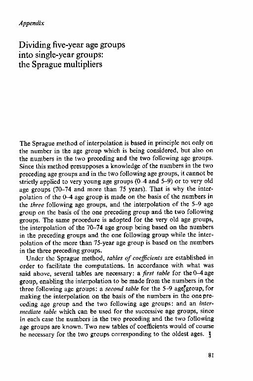
Appendix

Dividing five-year age groups into single-year groups: the Sprague multipliers

The Sprague method of interpolation is based in principle not only on the number in the age group which is being considered, but also on the numbers in the two preceding and the two following age groups. Since this method presupposes a knowledge of the numbers in the two preceding age groups and in the two following age groups, it cannot be strictly applied to very young age groups (O-4 and 5-9) or to very old age groups (70-74 and more than 75 years). That is why the interpolation of the O-4 age group is made on the basis of the numbers in the three following age groups, and the interpolation of the 5-9 age group on the basis of the one preceding group and the two following groups. The same procedure is adopted for the very old age groups, the interpolation of the 70-74 age group being based on the numbers in the preceding groups and the one following group while the interpolation of the more than 75-year age group is based on the numbers in the three preceding groups.

Under the Sprague method, tables of coeficients are established in order to facilitate the computations. In accordance with what was said above, several tables are necessary: a jirst table for the O-4 age group, enabling the interpolation to be made from the numbers in the three following age groups: a second table for the 5-9 agefgroup, for making the interpolation on the basis of the numbers in the onepre- ceding age group and the two following age groups: and an intermediate table which can be used for the successive age groups, since in each case the numbers in the two preceding and the two following age groups are known. Two new tables of coefficients would of course be necessary for the two groups corresponding to the oldest ages. 1

81

Appendix

An educational planner will especially need the first two tables and the intermediate table. These are given below.

If F, is the number in the age group under consideration, F+l, F+, and F,, the numbers in the three following age groups, and F-, and F-, the numbers in the two preceding age groups, and if, furthermore, F,, Fb, FC, Fd, and F, represent respectively the first, second, third, fourth and fifth age years of the group, the table of Sprague multipliers can be presented in the following form:

Sprague multipliers

First table F, Fb FC Fd F,

Second table F, Fb FC Fd F.

Intermediate table F, Fb FC Fd F.

+0.0336 +0.0080 -0.0080 -0.0160 -0.0176

-0.0128 t-0.0848 -0.0016 +0.0144 +0.0064 -0.0336 +0.0064 -0.0416 to.0016 -0.0240

+0.3616 +0.2640 +0.1840 -to.1200 f0.0704

+0.2272 +0.2320 $0.2160 +0.1840 -CO.1408

+0.1504 +0.2224 +0.2544 +0.2224 to.1504

-0.2768 -0.0960 +0.0400 -to.1360 +0.1968

-0.0752 -0.0480 -0.0080 $0.0400 $0.0912

-0.0240 -0.0416 -0.0336 +0.0144 t-O.0848

$0.1488 -0.0336 +0.0400 -0.0080 -0.0320 f0.0080 -0.0720 +0.0160 -0.0848 +0.0176

$0.0144 +0.0080 +o.oooo -0.0080 -0.0144

+0.0016 +0.0064 +0.0064 -0.0016 -0.0128

By way of illustration, the following is the procedure for estimating the numbers of children of 6,7, 89, 10 and 11 years when the numbers of individuals in the O-4, 5-9,10-14, 15-19 and 20-24 year age groups are known.

The given figures are the following:

04 age group: 161300 5-9 age group: 139515

10-14 age group: 71225 15-19 age group: 47300 20-24 age group : 38 820

82

Appendix

As has been noted above, to interpolate the 5-9 age group we will use the second table of Sprague multipliers, while the intermediate table will be used for the lo-14 age group (or any following age groups).

The number of 6-year-olds, for example, corresponds to line Fb in the second table above. Therefore :

Number of 6-year-olds = 0.0080 F-,+0.2320 F, -0.0480 F+,+0.0080 F,,

= (0.0080 x 161300)+(0.2320x 139515) - (0.0480 x 7 1225) +(O.OOSO x 47 300)

= 1290+32367-3419+378 = 30616

Estimate of numbers of children of 6, 7, 8 and 9 years of age

Age

6 7 8 9

161 300 139515 multiplied by multiplied by

corresponding corresponding coefficient coetlicient

+1290 +32 361 -1290 $30 135 -2 581 $-25 671 -2839 119644

71225 multiplied by

corresponding coefficient

-3 419 - 570 +2 849 16496

47 300 multiplied by

corresponding coefficient

+378 0

-378 -681

Total

30 616 28 275 25 561 22 620

Estimate of numbers of children of 10 and 11 years of age

161 300 139 515 71225 47 300 38 820 muliplied by multiplied by multiplied by multiplied by multiplied by

corresponding corresponding corresponding corresponding corresponding A& coefficient coefficient coefficient coefficient coeflicient Total

10 -2065 $11 831 $10712 -1135 + 62 19405 11 - 258 + 2009 +15 840 - 1 968 +248 15 871

83

Suggestions for further reading

I. General NC, L. K. Y. The population crisis. Bloomington, Indiana, Indiana Univer-

sity Press, 1965. THOMPSON, W. S. ; LEWIS, D. T. Population problems. New York, London,

McGraw-Hill, 1965.

II. Census UNITED NATIONS. Handbook of population census methods. New York.

(Studies in methods, ST/STAT/Ser. F/S/Rev. 1.) Vol. 1 General aspects of a population census. 1958. Vol. 2 Economic characteristics of the population. 1958. Vol. 3 Demographic and social characteristics of the population. 1959.

III. Methods of estimating UNITED NATIONS. Manuals on methods of estimating population. New York.

(Population studies.) Vol. 1 Methods of estimating total population for current dates. 1952.

(ST/SOA/Series A/10.) Vol. 2 Methods of appraisal of quality of basic data for population esti-

mates. 1955. (ST/SOA/Series A/23.) Vol. 3 Methods for population projections by sex and age. 1956. (ST/

SOA/Series A/25.) Vol. 4 Methods of estimating demographic measures from incomplete

data. 1967. (ST/SOA/Series A/42.) Lw, B. A. Estimating future school enrolment in developing countries: a

manual of methodology. New York, Unesco/United Nations, 1966. (Statistical reports and studies.) (Also in United Nations Population studies, 1966.) (ST/SOA/Series A/40.)

IIEP book list

The following books, published by Unesco/IIEP, are obtainable from the Institute or from Unesco and its national distributors throughout the world: Educational development in Africa (1969. Three volumes, containing eleven African

research monographs)

Educational planning: a bibliography (1964)

Educational planning: a directory of training and research institutions (1968)

Educational planning: an inventory of major research needs (1965)

Educational planning in the USSR (1968)

Fundamentals of educatiorial planning (series of booklets: full current list available on request)

Manpower aspects of educational planning (1968)

Methodologies of educational platining for developing countries by J. D. Chesswas (1969)

Monographies africaines (five titles, in French only: list available on request)

New educational media in action: case studies for planners (1967. Three volumes)

The new media: memo to educational planners by W. Schramm, P. H. Coombs, F. Kahnert, J. Lyle (1967. A report including analytical conclusions based on the above three volumes of case studies)

Problems and strategies of educational planning: lessons from Latin America (1965)

Qualitative aspects of educational planning (1969)

The following books, produced in but not published by the Institute, are obtainable through normal bookselling channels: Quantitative methods of educationalplanning by Hector Correa

Published by International Textbook Co., Scranton, Pa., 1969

The world educational crisis: a systems analysis by Philip H. Coombs Published by Oxford University Press, New York, London and Toronto, 1968

The International Institute for Educational Planning

The International Institute for Educational Planning (IIEP) was established by Unesco in 1963 to serve as an international centre for advanced training and research in the field of educational planning. Its basic financing is provided by Unesco and its physical facilities by the government of France. It also receives supplemental support from private and governmental sources.

The Institute’s aim is to expand knowledge and the supply of competent experts in educational planning in order to assist all nations to accelerate their educational development. In this endeavour the Institute co-operates with interested training and research organizations throughout the world.

The governing board of the Institute is as follows:

Chairman Sir Sydney Caine (United Kingdom), former Director, London School of Economics and Political Science

Members Hellmut Becker (Federal Republic of Germany), President, German Federation of Adult Education Centres

Alain Bienayme (France), Technical Adviser, Ministry of Education Roberto Campos (Brazil), former Minister of Economic Planning

and Development Richard H. Demuth (United States of America), Director,

Development Services Department, International Bank for Reconstruction and Development

Abdel-Aziz El-Koussy (United Arab Republic), Director, Regional Centre for Educational Planning and Administration in the Arab Countries

Joseph Ki-Zerbo (Upper Volta), President, National Commission of the Republic of Upper Volta for Unesco

D. S. Kothari (India), Chairman, University Grants Commission Philippe de Seynes (France), Under-Secretary-General for

Economic Social AtTairs, United Nations P. S. N. Prasad (India), Director, Asian Institute for Economic

Development and Planning S. A. Shumovsky (Union of Soviet Socialist Republics), Head,

Methodological Administration Department, Ministry of Higher and Specialized Secondary Education (RSFSR)

Fergus B. Wilson (United Kingdom) Chief, Agricultural Education Branch, Rural Institutions and Services Division, Food and Agriculture Organization of the United Nations

Inquiries about the Institute and requests for copies of its Progress Report 1963-67 should be addressed to: The Director, IIEP, 9 rue Eugene-Delacroix, 75 Paris-160

demographic aspects of educational planning -...

Documents