deﬁnition of a 4d continuous planispheric transformation ... · continuous planispheric...

Medical Image Analysis (1998) volume 4, number 1, pp 1–17c Oxford University Press

Definition of a 4Dcontinuous planispheric transformationfor the tracking and the analysis of LV motion

Jerome Declerck�, Jacques Feldmar and Nicholas Ayache

INRIA, Projet EPIDAURE2004 route des Lucioles, B.P. 9306 902 Sophia Antipolis Cedex, France

AbstractCardiologists assume that analysis of the motion of the heart (especially the left ventricle) cangive some information about the health of the myocardium.A 4D polar transformation is defined to describe the left ventricle (LV) motion and a methodis presented to estimate it from sequences of 3D images. The transformation is defined in 3D-planispheric coordinates (3PC) by a small number of parameters involved in a set of simplelinear equations. It is continuous and regular in time and space, periodicity in time can beimposed. The local motion can be easily decomposed intoa few canonical motions (radial motion,rotation around the long-axis, elevation). To recover the motion from original data, the 4D polartransformation is calculated using an adaptation of the Iterative Closest Point algorithm.We present the mathematical framework and a demonstration of its feasability on a series of gatedSPECT sequences.

Keywords: motion tracking, heart, LV, motion analysis, 4D

Received ?; revised ?; accepted ?

INTRODUCTION

Cardiologists assume that the analysis of the motion of theheart (especially the left ventricle) can give some informationabout the health of the myocardium. A huge effort has beenmade in medical image processing to track and analyse themotion of the LV, but due to the complexity of the modeling,this topic remains an open research problem.

Modern techniques provide 3D images which describe ei-ther the anatomy of the heart (MRI, US, for instance) or itsfunctionality (Nuclear Medicine SPECT or PET imaging, forinstance). It is possible to get sequences of such images overthe whole cardiac cycle; such sequences are real 3D movies ofthe motion of the heart. The cardiac motion, like the motionof any real object must be therefore described as a 4D con-tinuous and regular transformation of time and space. Withthe modality we are using for our experiments (gated SPECT),

�Corresponding author(e-mail: [email protected])

the acquisition of an image lasts over several cardiac cycles;the gating procedure allows to reconstruct a 3D volume usinginformation taken at similar times over different cardiac cy-cles, assuming that all the cycles are identical during the ac-quisition. In our protocol, we therefore suppose that the heartbeats at a regular pace, this may not be the case for specificpathologies inducing irregularities of the cardiac pulse rate:these diseases are not supposed to be studied in this paper.

Many techniques have been proposed to track the LV mo-tion. All of them attempt to find the correspondence be-tween pairs of successive images. Most of the proposedmethods in 3D define a model of the shape of LV surfaces(endocardium and/or epicardium), using classical snake-likemodels (McInerney and Terzopoulos, 1995; Shi et al., 1994;Amini and Duncan, 1992), spring-mass meshes (Nastar,1994) or more constrained generic surfaces such as free-deformed superquadrics (Bardinet et al., 1996; Bardinet et al.,1995) or volumetric superquadrics (Park et al., 1996; Parket al., 1994). The tracking is processed using conservation

2 J. Declerck et al.

constraints based on proximity constraints (Bardinet et al.,1996; Bardinet et al., 1995), differential properties of thesurface (Clarysse et al., 1995; Shi et al., 1994; Amini andDuncan, 1992; Goldgof et al., 1988) or is directly computedfrom displacement or velocity information obtained in somespecific MR imaging techniques: tags (Radeva et al., 1996;Kraitchman et al., 1995; Young et al., 1995; Denney andPrince, 1994; Park et al., 1994) or phase contrast (Meyer et al.,1995; Shi et al., 1995). In other work, no shape model iscomputed: the tracking is processed directly from the volu-metric image using optical flow methods (Gorce et al., 1997;Song et al., 1994), conservation of differential elements ofisophotes (Benayoun et al., 1995) or using similarities of theintensity levels (Thirion, 1995).

Unfortunately, because the correspondence is defined be-tween two successive images, regularity and periodicity intime is not guaranteed. Only a few studies impose tempo-ral continuity or periodicity in their model: these studiesdeal with segmentation of 2D (O’Donnell et al., 1994) or3D images (de Murcia, 1996; Matheny and Goldgof, 1995;Schudy and Ballard, 1979). Some other rare methods in 2D(Todd Constable et al., 1994; McEachen et al., 1994) or in3D (Thirion, 1995; Nastar, 1994) perform a posteriori timefiltering. Moreover, all these tracking techniques ((Park et al.,1996; Park et al., 1994) excepted) do not provide intuitive pa-rameters describing characteristic motions without non-trivialcomputation (Bardinet et al., 1996; Bardinet et al., 1995;Young et al., 1994). The 4D polar transformation (Declercket al., 1997) defined in this article aims to achieve four goals:

1. to define a class of transformation of time and space inwhich the temporal continuity and periodicity can beincluded,

2. to define a class of highly constrained transformationsin order to have a relevant description of the LV motionwith a reduced number of parameters,

3. to be able to retrieve canonical motions with minimalcomputation, providing an easy-to-interpret quantita-tive analysis of the motion.

4. last, but not least, to be a transformation which combinesthe unknown parameters in a linear way to make theirestimation easier and robust.

We shall see that all these points are achieved in the mathe-matical formulation that we propose below.

The paper is organised as follows: in section 1, we definethe 4D polar transformation and the way to estimate it from a4D (3D + time) data set. In section 2, a method is proposedto track in 4D the motion of the LV. Experiments have beenconducted with a synthetic heart model and a gated SPECT

sequence are presented in section 3. Section 4 draws con-clusions concerning this work, its potential uses and futureperspectives.

1. DEFINITION OF THE 4D PLANISPHERICTRANSFORMATION

The idea of this study is to define a continuous and regulartransformation of time and space. This transformation shouldalso be adapted to describe with a minimum of parameters acomplex motion such as the LV motion. This model of thedeformation of the LV is a crude approximation compared tocomplex biomechanical models (Hunter and Smaill, 1988) orhighly descriptive kinematic models (Arts et al., 1992).

Given a point P (x, y, z) in cartesian coordinates and atime value t, the transformation gives a point Q (x0, y0, z0)which is assumed to be the location of point P at time t. Thecardiac motion is supposed to be regular in space and periodicin time. We therefore look for a differentiable function inspatial variables x, y and z and for a differentiable and apotentially periodic function in time variable t.

f : IR3� IR �! IR3

(P; t) 7�! Q = f (P; t)

This definition of the 4D transformation yields the definitionof 2 categories of functions which are easier to understand andwhich are intrinsically regular (figure 1):

TP = f (P; �) is the trajectory of P over time;Dt = f (�; t) is the instantateneous deformation

function of the object at time t.

t nt 0

n

P

f (P ,t )

Q nQ 0

model

image sequence

Dt0

Dtn

T P

f (P ,t )0

Figure 1. The model is deformed at every time of the image se-quence. Point P at time tn is point Qn. Functions of instantaneousdeformation Dtn and the trajectory function TP are illustrated.

Definition of a 4D continuous planispheric transformation for the tracking and the analysis of LV motion 3

In this paper, f is defined in order to describe locally somespecific motions of points on the myocardium. We approx-imate the shape of the left ventricle as a stretched sphere inthe long-axis direction. This is, of course, a very crude ap-proximation as the shape of the heart is much more complex,however our goal is not a precise definition of the shape ofthe muscle, but a plausible discrimination of characteristicmotions.

For that particular purpose, we separate the motion of apoint of the heart into three canonical orthogonal motions(figure 2):

� motion 1: a radial motion which decribes the contrac-tion or dilatation of the whole structure towards a “cen-ter” ;

� motion 2: a apico-basal rotation around the apico-basal axis which describes the twisting motion of the LVpoints ;

� motion 3: a motion (tangential to the surface r = Ct )which describes the elevation of the LV points in theapico-basal direction (the shortening along the long-axisduring the systole).

P

C

P

C

P

P

2

3

1

21 3

3

C

C

P

P1

P2

Figure 2. The top three frames illustrate the orthogonal motionsdescribed in the text. Bottom, point P is transformed in P1 by thefirst motion (radial motion), P1 is transformed in P2 by the second(apico-basal rotation) and P2 is transformed in P3 by the third one(elevation).

We describe these motions in a “3D-planispheric” coordi-nates (3PC) system, which is a combination of spherical and

cylindrical coordinates. Our tranformation function is thusdefined as a composition of three functions:

f = P2C�F �C2P

The function C2P switches from cartesian to 3PC, P2Cswitches back from 3PC to cartesian coordinates (of course,C2P = P2C�1). F is the function which is described with thethree basic motions in 3PC. The next two paragraphs detail thedefinitions of these functions.

1.1. Cylindrical or planispheric coordinates ?The approach is inspired from (Park et al., 1996; Park et al.,1994): in that study, the equations for the deformation of thesuperquadric model is expressed in cylindrical coordinates. Insuch coordinates, the decomposition of the local motion in ourthree canonical motions does not have the same relevance ifthe point where they are estimated belongs to a lateral wall(where the muscle is roughly cylindrical) or if the point isclose to the apex (where the muscle is roughly spherical).For instance, a point belonging to a lateral wall and animatedby an axial contraction does effectively contract towards thecylindrical axis (motion 1), but a point close to the apex ani-mated with a similar motion does not contract, but undergoesa shift tangential to the wall. Thus, this motion is a twist(motion 2) or an elevation (motion 3) rather than a contraction(motion 1) (figure 3). We find it easier and more relevant to

C

long axis

P

P2

1

HP1

HP2

B

Figure 3. P1 belongs to a lateral wall, P2 is close to the apex, bothpoints are animated with motion 1. Solid arrows describe the mo-tion in cylindrical coordinates (contraction towards the apico-basalaxis) and dotted arrows describe the motion in spherical coordinates(contraction towards the center C). Motion 1 effectively describes acontraction for P1, but not for P2.

use 3D-planispheric coordinates rather than cylindrical onesto decompose the local motion of points of the myocardium.


1.2. 3D-Planispheric coordinatesC2P : in 3D cartesian space, we define a 3D-planisphericreference system given a center C, a base B and a set of twoorthogonal vectors u and v (figure 7). In order to fit with ourdescription of the heart, we choose u as a vector parallel tothe apico-basal direction, and v parallel to the septo-lateraldirection. C is chosen in the center of the cavity, and B in thecenter of the base.

For each point P (x, y, z), a center point HP is defined online (CB). From this center point, a distance and two angles(latitude θ and longitude φ) are calculated just as in the clas-sical spherical coordinate system. In the spherical system, HP

is the center C. In the cylindrical system, HP is the orthogonalprojection of P on the line CB. Our purpose here is to definea combination of both spherical and cylindrical coordinatesystems (figure 4), in order to describe the position of P in“roughly” spherical coordinates around the apex (where theshape of the LV is roughly spherical) and in “roughly” cylin-drical coordinates around the base (where the shape of the LVis roughly cylindrical). In our system, the position of HP onthe line CB is given by the simple formula:

CHP = (1� cosθ)CB (1)

Cylindrical Planispheric

CC

B

Spherical

Figure 4. 3D-planispheric geometry is a combination of both cylin-drical and spherical geometries.

� For low values of θ (P around the apex), HP is close toC and shifts away from C with a distance increasing with

θ2

2: around the apex, the 3PC system is thus close to the

spherical one.� For θ around π

2 (P around the apex), HP is close to B,the distance BHP varies linearly with θ� π

2 , and PHP

is nearly orthogonal to CB: around the base, the 3PCsystem is close to the cylindrical one (figure 7).

Of course, (1) is an implicit formula: HP gives the angle θ,but we need θ to locate HP. appendix A details the method wehave developed to compute the location of HP given a point Pin space.

In our 3PC system, a surface of constant r is representedas a disk in a plane, like in a classical map projection intopography (this is why we use the word “planispheric”). Thecoordinates X, Y and R in this system are defined as follows:

X =θπ

cos(φ)

Y =θπ

sin(φ) (2)

R =r

σr

where σr is a normalization coefficient so that X, Y and Rare dimensionless and vary within a similar range of values.Figure 5 illustrates the correspondence between the (x, y, z)

C

B

r

P

H

θ

XR

φP

θ

Y

φ

P

u

v

w

r

Figure 5. the cartesian coordinates (x,y,z) of point P are convertedinto polar coordinates in the 3D-planispheric image, the depth R isthe distance from the point HP in the cartesian image, the position(X ,Y) in the plane is defined with the two angles θ and φ, like in the2D-planispheric mapping.

cartesian coordinates and the (X, Y , R) coordinates in the 3PCsystem. In this system, apex point (X = 0, Y = 0) is the “southpole” of the projection, the points on the circle X2 +Y2 = 1(θ = π) are the same cartesian point, the “north pole” of theprojection, featuring a point in the direction of the base orof the aorta. Around this point, the distorsion between thecartesian and our planispheric representation is maximum, butthere should not be any cardiac points in this area (figure 6).


South pole

Lat.

Inf.myocardium

North pole

Sep.

B

CLat.

North pole circle

Ant.

Sep.

Figure 6. Left, the myocardium. From the center C, the limit ofthe basis draws a cone (dark gray) around the north pole. Right, inthe 3D-planispheric map, the left ventricle (light gray) appears like aplate, the cone is a circular stripe around the heart.

P2C : conversely, given a point (X, Y , R) in the 3PC systemso that X2 +Y2 � 1, we can compute its cartesian coordinates(x, y, z) by calculating θ = π

pX2 +Y2 and φ without ambigu-

ity with the expressions of cos(φ) and sin(φ). The center HP

is calculated with (1).The coordinate system we use is similar to the prolate

spheroidal coordinates (PSC) system described in the litter-ature (Waks et al., 1996). The equations are presented inappendix B, figure 7 shows ten surfaces of constant R in eachof the two systems. There are three minor differences betweenthe two systems:

1. the surfaces of constant R (for R values around whatthey should be to describe an average LV) are narroweraround the apex than in the 3PC system: the shape ofthese surfaces is closer to the shape of an average LV;

2. there is an interval of R for which surfaces of constant Rare close to a shape of an average LV. For those values,the location of point C is closer to the apex in the PSCsystem than in the 3PC, potentially yielding to forbiddenintersection of segment [CB] with the myocardial wall;

3. the surfaces of constant θ are cones in the 3PC system,they are confocal one-sheet hyperboloids in the PSCsystem. The local coordinates are orthogonal in PSC,whereas they are approximately orthogonal in 3PC. Onthe other hand, the decomposition of the motion is lessintuitive in the PSC system.

In the sequel of this article, we concentrate on the 3PC systemin order to obtain a closer approximation of the LV shape anda more intuitive decomposition of the motion.

vC

C’

B

u

P

u

BHPPH

Prolate spheroidal

vC

P

C’

Planispheric

Figure 7. A representation of ten surfaces of constant R, on the left,in the 3PC system, on the right, in the prolate spheroidal. The dashedlines show different curves of constant θ: on one, a point P and itsassociated center HP. Figure from (Declerck et al,1997).

1.3. The function in 3D-planispheric coordinatesIn the 3D-planispheric system, given a point P (X, Y , R), thetransformed point Q (X 0, Y 0, R0) through F is expressed asfollows:

X 0 = a0X�a1Y +a2

Y 0 = a1X +a0Y +a3 (3)

R0 = a4R+a5

X 0 and Y 0 are defined by a similarity function applied to X andY . A similarity is a combinate of a 2D rotation by angle α, auniform scaling of ratio k and a translation. R0 is defined as anaffine function of R. The similarity and the affine parametersap (p = 0 : : :5) are continuous and differentiable functions ofr, θ, φ and t.

Defining the transformation in the 3PC system allows towrite: a) linear expressions in the parameters ap, b) a simplecomputation of the canonical motion decomposition (radialmotion, rotation, elevation) from the ap and, c) a very compactdescription of the deformation.

1.3.1. Analysis of the motion in the canonical decompositionOur canonical motionsare retrieved with the following formu-lae:

1. the radial motion ratio (motion 1) is given by:

R0

R= a4 +

a5

R(4)


2. the linear relationships between X 0, Y 0 and X, Y define a2D similarity such that

k =q

a20 +a2

1 (5)

α = atan2(a1

k;

a0

k) (6)

α is the rotation around the long-axis (motion 2) in 3PC;

3. k is the scale factor corresponding to an elevation magni-fication in latitude, which is our motion 3. In our display,

we computeθ0�θ

θ.

The 4D polar transformation is defined once the parametersap are determined. Because of the simplicity of (5) and (6), itis possible to easily analyse the motion using the parametersap. Because the variation of the parameters ap is smoothand regular with variables r, θ, φ and t, the parameters whichdescribe our canonical motions are also smooth and regular intime and space.

1.3.2. Degrees of freedom of the parameters, time depen-dency as a hard constraint

In order to define a smooth and continuous 4D transformation,the parameters depend on the location of the point and theinstant at which the transformation is calculated. In our for-mulation, we choose the parameters as polynomial functionsin r and θ and quadratic periodic B-splines (Risler, 1991;Farin, 1989) in φ and t:

ap(r;θ;φ;t) =nr�1

∑i=0

nθ

∑j = 0j 6= 1

nφ�1

∑k=0

nt�1

∑n=0

Api; j;k;n

0@ r

σr

1A

i 0@θ

π

1A

j

BΦk (φ)BT

n (t) (7)

for p = 0 : : :4. If we keep for a5 an expression like (7), a4 and

a5 are correlated because R =r

σr. We therefore simplify a5

as follows:

a5(r;θ;φ; t)=nθ

∑j = 0j 6= 1

nφ�1

∑k=0

nt�1

∑n=0

A5j;k;n

0@θ

π

1A

j

BΦk (φ)BT

n (t) (8)

with the following notation:

� nr is the number of parameters which define the polyno-mial function of variable r: the degree of this polynomialis nr�1.

� nθ is the number of parameters which define the polyno-mial function of variable θ: to be differentiable in pointsfor which (θ = 0), the polynomial must have no termin θ (ap(θ) = a0

p + a2pθ2 + a3

pθ3 : : :). ap is therefore apolynomial of θ of degree nθ.

� nφ is the number of control points of the B-spline periodiccurve of variable φ. BΦ are the B-spline basis functionsassociated to a classical regularly distributed 2π-periodicset of knots.

� nt is the number of control points of the B-spline curve ofvariable t. BT are the B-spline basis functions associatedto a classical regularly distributed set of knots, this basiscan be periodic or not.

The originality of the transformation is in the fact that thecontinuity and potentially the periodicity in time is a “hard”constraint. We can implicitly look for time-periodic trans-formations.

Using quadratic B-splines (with a set of regularly dis-tributed knots in our current implementation) ensures C 1 con-tinuity in φ and t; the function ap(r;θ;φ; �) is a (potentiallyperiodic) piecewise polynomial. Due to the definition of B-splines, the influence of possible outliers remain local (Risler,1991).

To ensure the continuity for θ = 0, we must impose theconstraint Ap

i;0;k;n = Api;0;0;n for each k. There are thus nφ � 1

equations for each i and n. Finally, we get a number of controlpoints NCP = (5:nr +1):(nφ:(nθ�1)+1):nt.

The transformation is completely defined given a center Cand two orthogonal vectors (they define the 3PC system) anda set of NCP control points (real numbers) Ap

i; j;k;n .

1.4. Estimation of a 4D planispheric transformation1.4.1. The least squares criterionHaving a set of matches (Pl , Qn;l ) for different times tn (n =0 : : :T�1), we define a least squares criterion to estimate the4D planispheric transform which could “best” fit the list ofmatches:

8n 2 0 : : :N�1; 8m 2 0 : : :M�1;

f (Pl; tn) ' Qn;l (9)

The least squares criterion is therefore written:

J( f ) =T�1

∑n=0

N�1

∑l=0

αn;l :d( f (Pl; tn) ; Qn;l )2 (10)

where d(�; �) is the distance and αn;l is the weight related to thereliability of the match (Pl , Qn;l ).


If we choose the euclidean distance for d in cartesian co-ordinates, the criterion is not quadratic in the Ap

i; j;k;n, and itsderivatives with respect to the Ap

i; j;k;n are very difficult to lin-earize. We prefer to choose for d the euclidean distance ex-pressed in 3PC (X2+Y2+R2). The criterion is then quadraticin the Ap

i; j;k;n. d is a distance if and only if X2 +Y2 < 1 (i.e. iff(X,Y) does not belong to the circle of the “north pole” of theplanispheric map). As the center C is well inside the cavityand the base point B is in the center of the base circle, we aresure that all data points remain in a “security” cylinder in the3PC system (maximum expected value for θ is around π=2, soX and Y are less than 0:5. See figure 6).

1.4.2. Minimization of the criterionThe criterion expressed with d as the euclidean distance in3PC is quadratic in the control points Ap

i; j;k;n. Differentiatingit with respect to Ap

i; j;k;n gives a linear system which is solvedwith a classical conjugate gradient method. The size of thematrix is (5:nr + 1):(nφ:(nθ � 1) + 1):nt . In fact, the linearsystem can be split in two independent subsystems, one fora0, a1, a2, a3 and the other for a4 and a5.

Assembling the matrix is an operation which obviously de-pends linearly with the N, the number of matches. Solving thelinear system is an operation which depends on NCP , the sizeof the matrix : a classical conjugate gradient needs O(NCP

2)elementary operations per iteration. In our experiments, theO(N) operation is much more costly than the O(NCP

2) one(ratio is approximately 5:1).

2. TRACKING THE 4D MOTION OF THE LV

We define in this section an adaptation of the Iterative ClosestPoint algorithm (Besl and McKay, 1992; Zhang, 1994) whichgives an estimation of those matches for the least squaresminimization: it is possible this way to calculate the “best”function with respect to a distance criterion.

The motion is tracked in a heart image sequence (in ourexperiments, gated SPECT). Points featuring the edges of theheart are extracted and matched. The result of the matchesbetween pairs of points in the images of the sequence is usedto estimate a 4D polar transformation.

2.1. Matching the feature pointsThe matching method is an enhancement of the iterative clos-est point (Besl and McKay, 1992; Zhang, 1994; Feldmar andAyache, 1996), adapted to our problem. Given a point P (x,y, z) in cartesian coordinates and a time value t, the transfor-mation gives a point Q (x0, y0, z0) which is assumed to be thelocation of point P at time t. To estimate a 4D planispherictransformation f , we therefore need to know the matches be-

tween points Pl of the first image (t = 0) and points Qn;l of theimage at time n (t = tn). We thus look for f so that

f (Pl; tn)'Qn;l

We define a criterion:

C( f ) =T�1

∑n=0

N�1

∑l=0

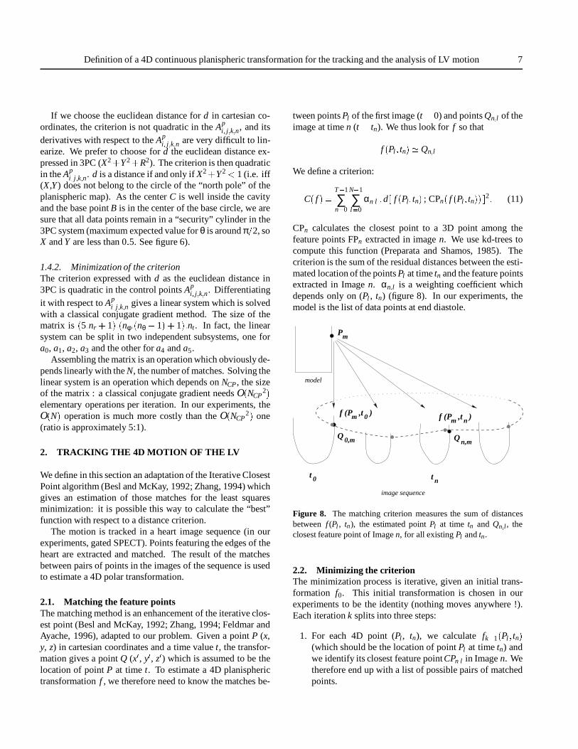
αn;l :d[ f (Pl; tn) ; CPn( f (Pl; tn)) ]2: (11)

CPn calculates the closest point to a 3D point among thefeature points FPn extracted in image n. We use kd-trees tocompute this function (Preparata and Shamos, 1985). Thecriterion is the sum of the residual distances between the esti-mated location of the points Pl at time tn and the feature pointsextracted in Image n. αn;l is a weighting coefficient whichdepends only on (Pl , tn) (figure 8). In our experiments, themodel is the list of data points at end diastole.

t

image sequence

nt 0

mf (P ,t )0

Pm

mf (P ,t )n

Q n,mQ 0,m

model

Figure 8. The matching criterion measures the sum of distancesbetween f (Pl , tn), the estimated point Pl at time tn and Qn;l , theclosest feature point of Image n, for all existing Pl and tn.

2.2. Minimizing the criterionThe minimization process is iterative, given an initial trans-formation f0. This initial transformation is chosen in ourexperiments to be the identity (nothing moves anywhere !).Each iteration k splits into three steps:

1. For each 4D point (Pl , tn), we calculate fk�1(Pl; tn)(which should be the location of point Pl at time tn) andwe identify its closest feature point CPn;l in Image n. Wetherefore end up with a list of possible pairs of matchedpoints.


2. For each time tn and for each type of boundary (en-docardium, epicardium), we calculate the residual dis-tance k fk�1(Pl; tn)�CPn;lk for each pair, and we decidewhether a pair is reliable or not: we first eliminate pairsfor which the residual distance exceeds a fixed threshold.Second, we compute the mean µ and the standard devia-tion σ attached to the remaining pairs. We then eliminatethe points for which the distance is greater than anotherthreshold depending on the distance distribution (µ +c:σ, where c can be easily set using a χ2 table (Feldmarand Ayache, 1996; Feldmar, 1995)).

We get for this iteration a list Sk of reliable pairs ofmatched points. Notice that if a point is not matched inthis iteration, it may be matched in one that follows.

3. With the filtered list Sk of pairs of points, we calculate fk

which is the best least squares fit for the pairs of points.

The iterative process stops when a maximum number of iter-ations is reached, or when Sk = Sk�1. (Feldmar and Ayache,1996; Feldmar, 1995) gives further details about this adapta-tion of the iterative closest point algorithm, for instance aboutthe convergence properties.

2.3. Definition of the closest pointThe matching function CPn takes into account for each pointits geometric position and the local direction of the intensitygradient calculated while extracting the edges. Considering 2oriented points (P;nP) and (Q;nQ), where nP and nQ are the di-rections of the intensity gradient at point P and Q respectively,the distance between them is calculated as follows:

d(P;Q)2 = α:kPQk2 +knP�nQk2 (12)

where α is a weighting coefficient for normalisation. Thelocal direction of the gradient defines which border a pointsbelongs to: if the gradient is oriented towards the center, thepoint belongs to the endocardium. If not, it is assumed tobelong to the epicardium. This separation avoids mismatchesbetween points of two different boundaries and speeds up thecomputation: one kd-tree is more costly to manipulate thantwo kd-trees of half size.

This double definition of a point (location + direction) re-fines the matching criterion and makes it more robust and pre-cise. We know that such features must be used with caution,especially when trying to define a distance between two fea-tures (Pennec and Ayache, 1996). However, the formula (12)must be written as a sum of squares in order to keep theconvergence properties of the process (Feldmar and Ayache,1996; Feldmar, 1995).

2.4. Computing an optimal 3D-planispheric coordinatesystem

A keypoint in the estimation of the 4D transformation is thedefinition of a 3PC system (a center, a base, an apico-basalvector, a septo-lateral vector and a normalisation factor σr).

2.4.1. The coordinate systemIn (Declerck et al., 1996), we define a method to align aSPECT heart image with a template using a non-rigid trans-formation. This method gives a transformation from the nor-malized coordinates of the template to the patient’s case.

As the transformation which deforms the template is suf-ficiently free (B-spline tensor product), the template can bechosen as a rough approximation of a LV. Here, we choosetwo truncated ellipsoids (one for the endocardium and one forthe epicardium). The parameters have been set manually notto design a precise shape: the idea is just to have a “good-looking” one. We define for this template a center, a basispoint and a point in the lateral wall so that all three define areference system [C, u, v].

The template is matched with the edges of the image ofthe heart at end diastole (largest volume). With this trans-formation, we deform the reference system of the template tothe patient case (figure 9). Calling S (for “shape”) the spline

PPL

uP

deformed template

C v

Pw

BP

PC

T

w

Tu

original template

S

T

B

T

TvTL

Figure 9. The template and three points defining the coordinatesystem. By the transformation S, they are deformed to match theshape of the left ventricle of the patient.

transformation deforming the template to the patient’s case,the reference system is defined as follows:

� For the template

– center: CT

– base: BT

– lateral point : LT

– apicobasal vector : uT =CTBT

kCTBTk


– septo-lateral vector : vT =CT LT

kCT LTk(LT is such that uT :vT = 0)

– infero-anterior vector : wT = uT � vT

� For the patient’s case

– center : CP = S(CT )

– base : BP = S(BT )

– lateral point : LP = S(LT )

– apicobasal vector : uP =CPBP

kCPBPk– septo-lateral vector :

vP =CPLP�< uPjCPLP > :uP

k : : :k(so that uP:vP = 0)

– infero-anterior vector : wP = uP� vP

2.4.2. Choosing σr

The normalisation factor σr is used to make the R coordinatedimensionless, as are the other coordinates X andY . Changingσr changes the shape of a surface in the planispheric geometryby a scaling in the R direction (the lower σr, the “higher” thesurface). The closest point in this surface to a given point Pvaries with σr (figure 10):

� When σr approaches 0, the R value becomes very largecompared to X and Y , Q0, the closest point to P tends toa point with the same R (figure 10, left). This impliesthat if we use those matches for the least square criterionon distances, the tangential motions (those which changeonly X and Y) are privileged and the radial motion (thosewhich change only R) becomes negligible.

� When σr tends to infinity, the R value becomes verysmall compared to X and Y . Q∞, The closest point toP is a point with same X and Y (figure 10, right). Thisimplies that if we use those matches for the least squarecriterion on distances, the radial motion is privileged andthe tangential motions are negligible.

Giving a value to this factor therefore amounts to choosinga weighting between purely tangential and purely radial mo-tions.

As the latitude of the basal points approaches π=2, the abso-lute values of X and Y do not exceed 0:5. For an average heart,it appears that the maximum distance (meaning the r value) ofa point of the myocardium to the axis does not exceed CB. Wethus choose σr = 2:CB, so that R does not exceed 0:5 as for Xand Y .

o

oo

Po

Q

Q0

R

Y

XS

Y

R

Y

S

0R

XQ

XS

Q

rσ 0 r

σ oo

P

P

Figure 10. The surface S is represented in 3PC. In this geometry,the location of the closest point Q to P of surface S depends on σr.Q belongs to the curved segment [Q0Q∞], where Q0 and Q∞ are theclosest point to P for σr = 0 and ∞ respectively. Figure reprinted withkind permission of IEEE Trans. on Med. Imag.

3. EXPERIMENTS

We present here experiments conducted on a series of gatedSPECT image sequences provided by Pr. M.L. Goris, StanfordUniversity Hospital (California, USA). There are 8 images inthe sequence, the size of the images is 64x64x64, pixel sizeis 2.5mm isotropic. The temporal sampling is uniform andcovers the entire cardiac cycle.

3.1. Extraction of feature pointsEach image of the sequence is resampled in the polar geome-try defined in (Declerck et al., 1996). This reference describesa method to extract edges in nuclear medicine myocardialperfusion images, we recall here the main ideas: in a polargeometry with a center well inside the cavity, the heart lookslike a thick plate. We detect edges in this image with a Canny-


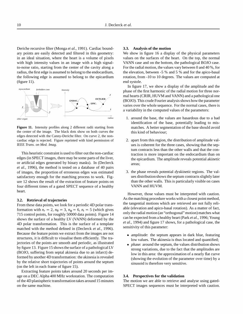
Deriche recursive filter (Monga et al., 1991). Cardiac bound-ary points are easily detected and filtered in this geometry:in an ideal situation, where the heart is a volume of pixelswith high intensity values in an image with a high signal-to-noise ratio, starting from the center of the cavity along aradius, the first edge is assumed to belong to the endocardium,the following edge is assumed to belong to the epicardium(figure 11).

myocardium

2

radius

OUTLIER

EPIC.ENDOC.

2

1

forbidden cone

other organ

Intensity

1

Figure 11. Intensity profiles along 2 different radii starting fromthe center of the image. The black dots show on both curves theedges detected with the Canny-Deriche filter. On curve 2, the non-cardiac edge is rejected. Figure reprinted with kind permission ofIEEE Trans. on Med. Imag.

This heuristic constraint is used to filter out the non-cardiacedges (in SPECT images, there may be some parts of the liver,or artificial edges generated by binary masks). In (Declercket al., 1996), the method is tested on a database of 40 pairsof images, the proportion of erroneous edges was estimatedsatisfactory enough for the matching process to work. Fig-ure 12 shows the result of the extraction of feature points onfour different times of a gated SPECT sequence of a healthyheart.

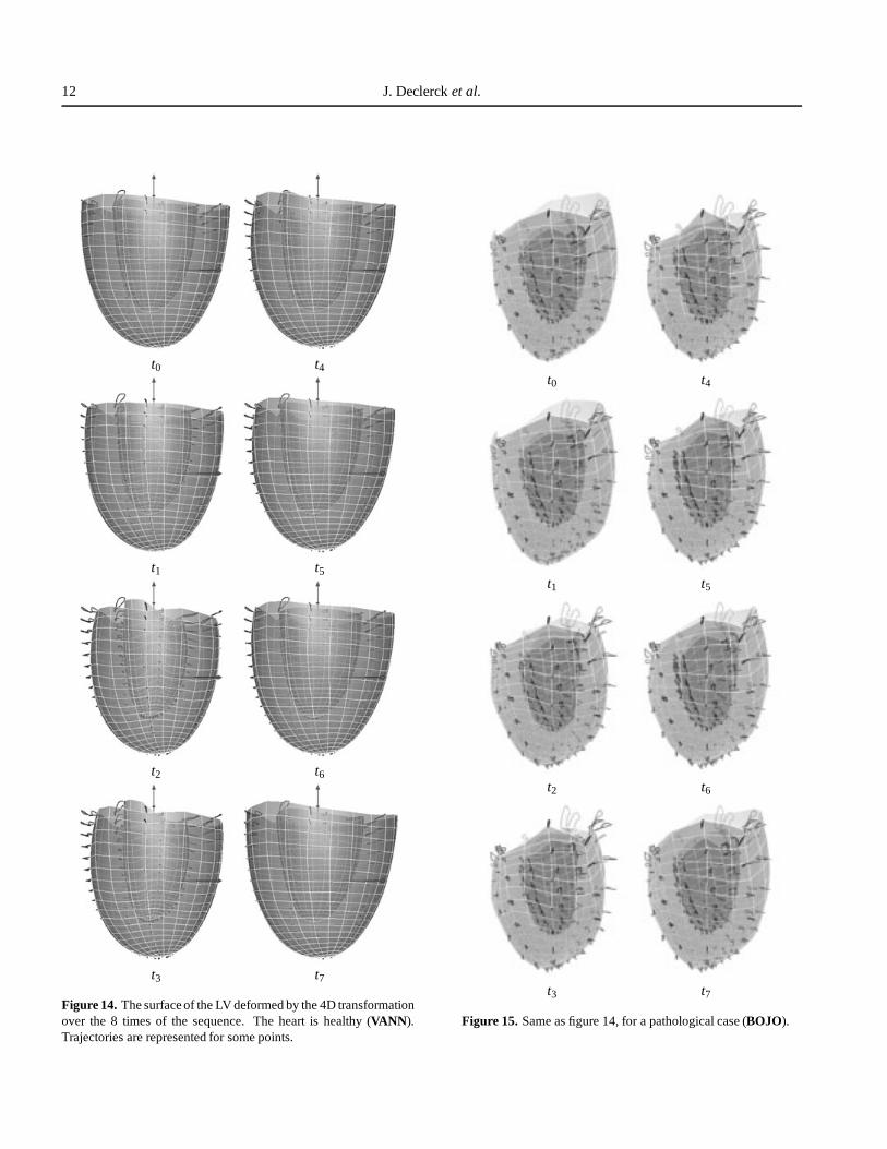
3.2. Retrieval of trajectoriesFrom these data points, we look for a periodic 4D polar trans-formation with nr = 2, nθ = 3, nφ = 6, nt = 5 (which gives715 control points, for roughly 50000 data points). Figure 14shows the surface of a healthy LV (VANN) deformed by the4D polar transformation. This is the surface of a templatematched with the method defined in (Declerck et al., 1996).Because the feature points we extract from the images are notstructures, it is difficult to visualise them efficiently. The tra-jectories of the points are smooth and periodic, as illustratedby figure 13. Figure 15 shows the surface of a pathological LV(BOJO, suffering from septal akinesia due to an infarct) de-formed by another 4D transformation: the akinesia is revealedby the relative short trajectories of points around the septum(on the left in each frame of figure 15).

Extracting feature points takes around 20 seconds per im-age on a DEC Alpha 400 MHz workstation. The computationof the 4D planispheric transformation takes around 15 minuteson the same machine.

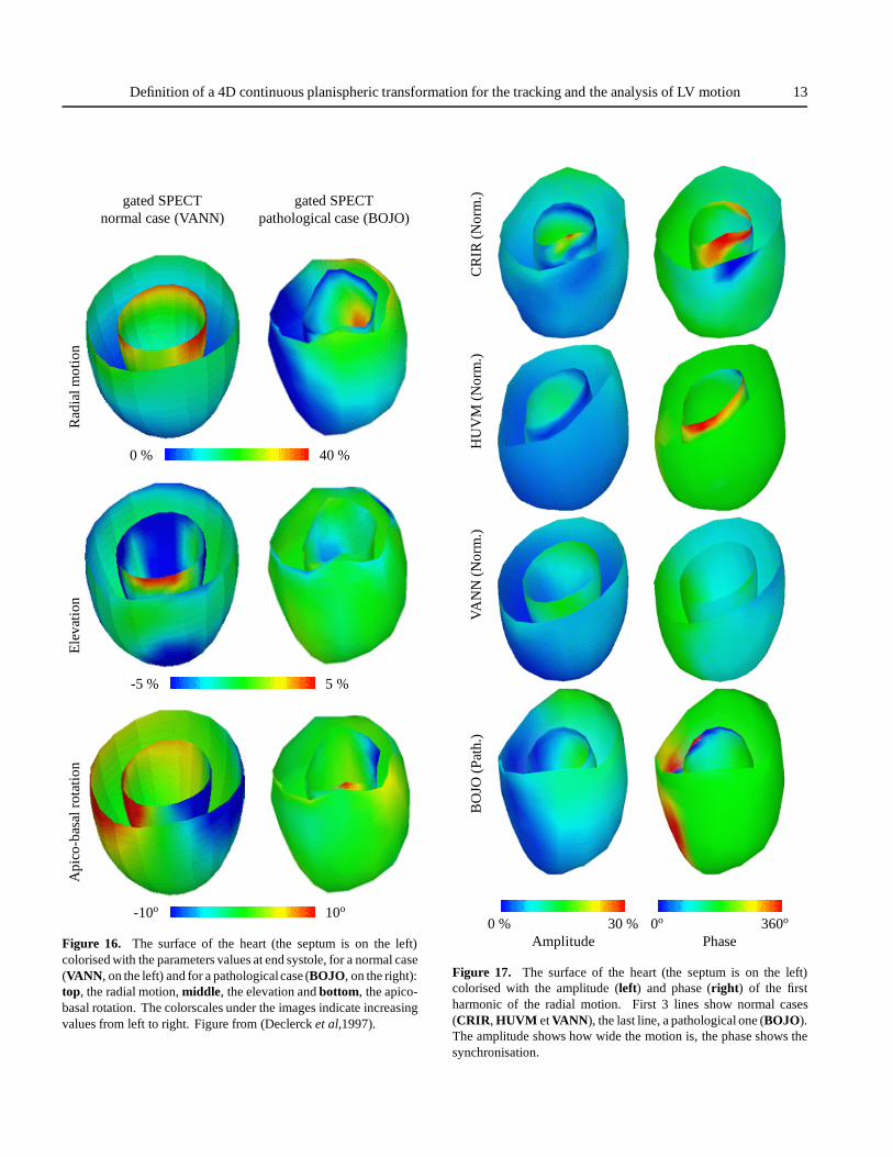
3.3. Analysis of the motionWe show in figure 16 a display of the physical parametersvalues on the surfaces of the heart. On the top, the normalVANN case and on the bottom, the pathological BOJO case.For the radial motion, the values vary between 0 and 40 %, forthe elevation, between -5 % and 5 % and for the apico-basalrotation, from -10 to 10 degrees. The values are computed atend systole.

In figure 17, we show a display of the amplitude and thephase of the first harmonic of the radial motion for three nor-mal hearts (CRIR, HUVM and VANN) and a pathological one(BOJO). This crude Fourier analysis shows how the parametervaries over the whole sequence. For the normal cases, there isa variability in the computed values of the parameters:

1. around the base, the values are hasardous due to a badidentification of the base, potentially leading to mis-matches. A better segmentation of the base should avoidthis kind of behaviour;

2. apart from this region, the distribution of amplitude val-ues is coherent for the three cases, showing that the sep-tum contracts less than the other walls and that the con-traction is more important on the endocardium than onthe epicardium. The amplitude reveals potential akineticareas;

3. the phase reveals potential dyskinetic regions. The val-ues distributionshows the septum contracts slightly laterthan the other walls. This is particularly visible on casesVANN and HUVM.

However, those values must be interpreted with caution.As the matching procedure works with a closest point method,the tangential motions which are retrieved are not fully reli-able (elevation and apico-basal rotation). As a matter of fact,only the radial motion (an “orthogonal” motion) matches whatcan be expected from a healthy heart (Park et al., 1996; Younget al., 1994) and figure 17 shows, for a pathological case, thesensitivity of this parameter:

� amplitude: the septum appears in dark blue, featuringlow values. The akinesia is thus located and quantified;

� phase: around the septum, the values distribution showsstrong variations, due to the fact that the amplitudes arelow in this area: the approximation of a nearly flat curve(showing the evolution of the parameter over time) by asinusoid is therefore very sensitive.

3.4. Perspectives for the validationThe motion we are able to retrieve and analyse using gated-SPECT images sequences must be interpreted with caution.


septum on left, lateral on right .. . lateral on left, septum on right

inferior on left, anterior on right

12

Septum Lateral

Inferior

Anterior

43

t0

t2

t4

t6

Figure 12. Edges (in white) automatically extracted and filtered from images at four different times (one time per row). On each row, we seecentral slices resampled from the 3D image by rotation around the apex-base axis, as shown on drawing on the left: this makes easier the displayof the myocardial structure.

Figure 13. View of the LV from the apex. The trajectories of some points are drawn over the cycle: they are smooth and periodic (see thezoomed area on the right). Figure from (Declerck et al,1997).


t0 t4

t1 t5

t2 t6

t3 t7

Figure 14. The surface of the LV deformed by the 4D transformationover the 8 times of the sequence. The heart is healthy (VANN).Trajectories are represented for some points.

t0 t4

t1 t5

t2 t6

t3 t7

Figure 15. Same as figure 14, for a pathological case (BOJO).


gated SPECT gated SPECTnormal case (VANN) pathological case (BOJO)

Rad

ialm

otio

n

0 % 40 %

Ele

vati

on

-5 % 5 %

Api

co-b

asal

rota

tion

-10o 10o

Figure 16. The surface of the heart (the septum is on the left)colorised with the parameters values at end systole, for a normal case(VANN, on the left) and for a pathological case (BOJO, on the right):top, the radial motion, middle, the elevation and bottom, the apico-basal rotation. The colorscales under the images indicate increasingvalues from left to right. Figure from (Declerck et al,1997).

CR

IR(N

orm

.)H

UV

M(N

orm

.)V

AN

N(N

orm

.)B

OJO

(Pat

h.)

0 % 30 % 0o 360o

Amplitude Phase

Figure 17. The surface of the heart (the septum is on the left)colorised with the amplitude (left) and phase (right) of the firstharmonic of the radial motion. First 3 lines show normal cases(CRIR, HUVM et VANN), the last line, a pathological one (BOJO).The amplitude shows how wide the motion is, the phase shows thesynchronisation.


Due to the low resolution of the images, it is difficult to get aprecise information. Second, any tangential motion cannot bereliably retrieved using only feature-based techniques withoutmarkers. The parameters we are able to compute may beuseful if there is a possibility to demonstrate that they can beused for a detection of a pathology, by separating normal andabnormal hearts into two statistically different classes. Thisvalidation should be processed on a dataset of heart images ofwhich the pathology or healthy state is known. For a givendatabase, the sensitivity and the specificity can be calculatedand can show the usefulness of our approach on a quantitativebasis.

Another way to validate our decomposition of the motionis to check that it corresponds to a real motion. Tagged MRIyields images in which the motion of soft tissues at a num-ber of discrete points is easily detectable, can be measured(McVeigh, 1996; Kraitchman et al., 1995; Young et al., 1995;Young et al., 1994; Denney and Prince, 1994) and then com-pared to our computed motion.

These two validation processes are currently under study,partial results have been obtained (Declerck, 1997) and willbe the subject of a forthcoming article.

4. CONCLUSION

In this work, the mathematical framework for a new class oftransformation is defined: a 4D planispheric transformationis a differentiable function in space and time coordinates andpotentially periodic in time. A small number of parametersconstrain the definition of the function and there is a sim-ple relationship between the estimated parameters ap and the“canonical” motions defined for a moving LV (radial motion,rotation, elevation). We demonstrated the feasability of themethod on a series of gated SPECT sequences.

This will be the basis for a number of experimental studiesboth on nuclear medicine and tagged MR data in collaborationwith Pr. Michael Goris (Stanford University Hospital) andDr. Elliot McVeigh (Johns Hopkins University).

In order to refine the tracking procedure, we are also work-ing on defining feature points inside the myocardium. Thosepoints added to the edges we have already defined will givelandmarks in the entire myocardial volume and not only onits boundary.

ACKNOWLEDGEMENTS

We want to thank Pr. Michael L. Goris for his precious ad-vices we had and the team of the Stanford University Hospital(California, USA) for providing us with the images.

We give also special thanks to Dr. Eric Bardinet and Pr.Mike Brady for the constructive discussions and comments

about the project.This work was partially supported by regional grant of the

Region Provence Alpes Cote d’Azur (doctoral research con-tract).

A. 3D PLANISPHERIC COORDINATES

This section is dedicated to the problem of finding HP given apoint P in space. In order to avoid cumbersome notation, werename HP as H. The problem is, given two points C and Band a point P, to find a point H on the line CB so that:

(BC;HP) = θCH = (1� cosθ):CB

Let us define λ as follows:

CH = λ:CB = λ:l

Because λ is supposed to be equal to 1� cos(θ), λ 2 [0;2].If we write

CP =

0@

x:ly:lz:l

1A and u =

0@

ux

uy

uz

1A

we have

HP = l:

0@

x�λ:ux

y�λ:uy

z�λ:uz

1A

so

u:HP = u:HC+u:CP

= l:[�λ+(x:ux+ y:uy + z:uz)]

On the other hand,

cos(θ) =BC:HP

kBCk:kHPk

If we call

r = kHPk= l:

q(x�λ:ux)2 +(y�λ:uy)2 +(z�λ:uz)2

and

p = u:CP


we thus have

cos(θ) = �u:HPr

and the constraint (1) can be rewritten, after some calculation,

λ =r+ pr+1

(13)

Let us call f a function of λ

f (λ) =r(λ)+ pr(λ)+1

�λ (14)

We look for λ0 so that

f (λ0) = 0 (15)

To solve this equation, we use a Newton method. In thefollowing lines, we demonstrate that the derivative f 0 is of aconstant sign, which implies a unique solution for (15), if itexists.

The derivative of the function f with respect to λ is asfollows

f 0(λ) =r0(λ)(1� p)(r(λ)+1)2 �1

It is straightforward to prove that

r0(λ) =λ� pr(λ)

so we have

f 0(λ) =(λ� p)(1� p)r(λ)(r(λ)+1)2 �1 (16)

Let us call P0 is the projection of P on (CB). We have then

λ� p = �HP0

l

1� p = �BP0

l

To prove the constant sign of f 0, we just have to comparethe two distance products CB:HP0:BP0 (the numerator of the

P’ CB

B

H

C

P’

B

C

P

H

P’ P

P’ CB

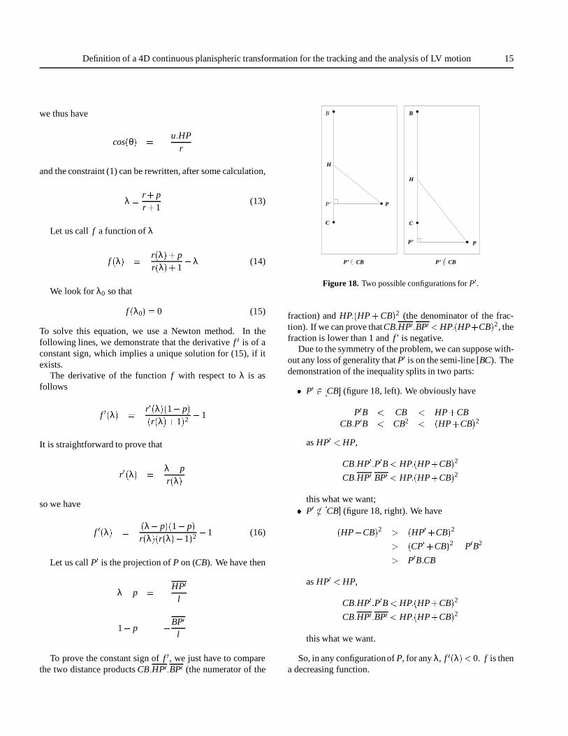
Figure 18. Two possible configurations for P0.

fraction) and HP:(HP+CB)2 (the denominator of the frac-tion). If we can prove that CB:HP0:BP0 <HP:(HP+CB)2, thefraction is lower than 1 and f 0 is negative.

Due to the symmetry of the problem, we can suppose with-out any loss of generality that P0 is on the semi-line [BC). Thedemonstration of the inequality splits in two parts:

� P0 2 [CB] (figure 18, left). We obviously have

P0B < CB < HP+CBCB:P0B < CB2 < (HP+CB)2

as HP0 < HP,

CB:HP0:P0B < HP:(HP+CB)2

CB:HP0:BP0 < HP:(HP+CB)2

this what we want;� P0 =2 [CB] (figure 18, right). We have

(HP+CB)2 > (HP0+CB)2

> (CP0+CB)2 = P0B2

> P0B:CB

as HP0 < HP,

CB:HP0:P0B < HP:(HP+CB)2

CB:HP0:BP0 < HP:(HP+CB)2

this what we want.

So, in any configurationof P, for any λ, f 0(λ)< 0. f is thena decreasing function.


Obviously,

f (0) =CP+u:CPCP+CB

> 0

and, if P0 is on the semi-line [BC),

f (1) =BP+u:CPBP+CB

�1

=u:CP�CBBP+CB

=u:BP

BP+CB< 0

f (0) and f (1) are of opposite signs, the sign f 0 is constant,there is then a unique solution for (15).

In our implementation, we use a Newton method to findλ0 solution of (15). Starting from a central position (λ = 1),after 3 or 4 iterations, the difference between two successiveestimations of λ do not exceed 10�6. The convergence isextremely fast.

B. PROLATE SPHEROIDAL COORDINATES

We define a center O and two “focal points” F1 and F2, F2being at the same distance δ from O as F1, but in the oppositedirection. A prolate sphere is defined to have a constant radiusλ (dimensionless number), a point in this prolate sphere isdefined fixing two angles: elevation θ and azimuth φ. Fromthese three parameters, the cartesian coordinates (x, y, z) ofthis pont are calculated using the following formulae:

x = δ sinh(λ) sin(θ) cos(φ)y = δ sinh(λ) sin(θ) sin(φ) (17)

z = δ cosh(λ) cos(θ)

Conversely, knowing the cartesian coordinates (x, y, z), it ispossible to compute the prolate spheroidal parameters (λ,θ,φ)using the equations:

r1 =q

x2 + y2 +(z�δ)2

r2 =q

x2 + y2 +(z+δ)2

λ = acosh

0@ r1 + r2

2:δ

1A

θ = acos

0@ r1� r2

2:δ

1A (18)

φ = atan2

0@ x

δ sinh(λ) sin(θ);

yδ sinh(λ) sin(θ)

1A

Analogously to our system, F1 would be C, O would be B,F2 would be C0 (figure 7) and λ would be R. In the end, thetransformation from (R,θ,φ) coordinates to (X,Y ,R) would beexpressed as in (2).

REFERENCES

Amini, A. and Duncan, J. (1992). Bending and stretching models forLV wall motion analysis from curves and surfaces. In Image andVision Computing, Vol. 10, pp. 418–430.

Arts, T., Hunter, W.C., Douglas, A., Muijtjens, A.M., and Reneman,R.S. (1992). Description of the deformation of the left ventricleby a kinematic model. Journal of Biomechanics, 25(10), 1119–1127.

Bardinet, E., Cohen, L.D., and Ayache, N. (1995). Tracking medical3D data with a parametric deformable model. In IEEE ComputerVision Symposium.

Bardinet, E., Cohen, L.D., and Ayache, N. (1996). Tracking and mo-tion analysis of the left ventricle with deformable superquadrics.Medical Image Analysis, 1(2), 129–149. (also INRIA researchreport #2797).

Benayoun, S., Nastar, C., and Ayache, N. (1995). Dense non-rigidmotion estimation in sequences of 3D images using differentialconstraints. In Computer Vision, Virtual Reality and Robotics inMedicine, Vol. 905 of Lecture Notes in Computer Science, pp.309–318. Springer-Verlag.

Besl, P. and McKay, N. (1992). A method for registration of 3Dshapes. IEEE Transactions on Pattern Analysis and MachineIntelligence, 14, 239–256.

Clarysse, P., Jaouen, O., Magnin, I., and Morvan, J.M. (1995).3D Boundary Extraction of the Left Ventricle by a DeformableModel with a priori Information. In IEEE International Confer-ence on Image Processing.

de Murcia, J. (1996). Reconstruction d’images cardiaques en tomo-graphie d’emission monophotonique a l’aide de modeles spatio-temporels. Ph.D. Thesis, Institut National Polytechnique deGrenoble.

Declerck, J. (1997). Etude de la dynamique cardiaque par analysed’images tridimensionnelles. Ph.D. Thesis, Universite Nice-Sophia Antipolis.

Declerck, J., Feldmar, and Ayache, N. (1997). Definition of a 4Dcontinuous polar transformation for the tracking and the anal-ysis of LV motion. In Computer Vision, Virtual Reality andRobotics in Medicine II - Medical Robotics and Computer As-sisted Surgery III, Vol. 1205 of Lecture Notes in Computer Sci-ence, pp. 33–42. Springer-Verlag.

Declerck, J., Feldmar, J., Goris, M.L., and Betting, F. (1996). Auto-matic registration and alignment on a template of cardiac stress


& rest SPECT images. In Mathematical Methods in BiomedicalImage Analysis, pp. 212–221. (Also INRIA Research Report# 2770. Accepted for publication in IEEE Transactions on Med-ical Imaging).

Denney, T.S. and Prince, J.L. (1994). 3D displacement field re-construction from planar tagged cardiac MR images. In IEEEWorkshop on Biomedical Image Analysis, pp. 51–60.

Farin, G. (1989). Curves and Surfaces for Computer Aided Geomet-ric Design. Academic Press, Inc.

Feldmar, J. (1995). Recalage rigide, non-rigide et projectif d’imagesmedicales tridimensionnelles. Ph.D. Thesis, Ecole Polytech-nique.

Feldmar, J. and Ayache, N. (1996). Rigid, affine and locally affineregistration of free-form surfaces. Computer Vision and ImageUnderstanding, 18(2), 99–119. (Also INRIA Research Report# 2220).

Goldgof, D., Lee, H., and Huang, T. (1988). Motion analysis of non-rigid surfaces. In IEEE Computer Vision and Pattern Recogni-tion, pp. 375–380.

Gorce, J.M., Friboulet, D., and Magnin, I.E. (1997). Estimation ofthree-dimensional cardiac velocity fields: assessmentof a differ-ential method and application to 3-D CT data. Medical ImageAnalysis, 1(3), 1–16.

Hunter, P.J. and Smaill, B.H. (1988). The analysis of cardiac func-tion: a continuum approach. Prog. Biophys. Molec. Biol., 52,101–164.

Kraitchman, D., Young, A., Chang, C.N., and Axel, L. (1995). Semi-automatic tracking of myocardial motion in MR tagged images.IEEE Transactions on Medical Imaging, 14(3), 422–433.

Matheny, A. and Goldgof, D. (1995). The use of three- and four-dimensional surface harmonics for rigid and nonrigid shape re-covery and representation. IEEE Transactions on Pattern Anal-ysis and Machine Intelligence, 17(10), 967–978.

McEachen, J.C., Nehorai, A., and Duncan, J.S. (1994). A recursivefilter for temporal analysis of cardiac motion. In IEEE Workshopon Biomedical Image Analysis, pp. 124–133.

McInerney, T. and Terzopoulos, D. (1995). A dynamic finite elementsurface model for segmentationand tracking in multidimensionalmedical images with application to cardiac 4D image analysis.Computerized Medical Imaging and Graphics, 19(1), 69–83.

McVeigh, E. (1996). MRI of myocardial function: motion trackingtechniques. Magnetic Resonance Imaging, 14(2), 137–150.

Meyer, F.G., Todd Constable, R., Sinusas, A., and Duncan, J. (1995).Tracking myocardial deformation using spatially-constrainedvelocities. In et al., Y. Bizais (ed.), Information Processing inMedical Imaging, pp. 177–188.

Monga, O., Deriche, R., and Rocchisani, J.M. (1991). 3D edge de-tection using recursive filtering: application to scanner images.Computer Vision, Graphicsand Image Processing,53(1), 76–87.

Nastar, C. (1994). Vibration modes for non-rigid motion analysisin 3D images. In European Conference in Computer Vision,number 800 in Lecture Notes in Computer Science, pp. 231–236.Springer-Verlag.

O’Donnell, T., Gupta, A., and Boult, T. (1994). A periodic general-ized cylinder model with local deformations for tracking closed

contours exhibiting repeating motion. In IEEE Workshop onBiomedical Image Analysis, pp. 397–402.

Park, J., Metaxas, D., and Axel, L. (1996). Analysis of left ventric-ular motion based on volumetric deformable models and MRI-SPAMM. Medical Image Analysis, 1(1), 53–71.

Park, J., Metaxas, D., and Young, A. (1994). Deformable modelswith parameter functions: application to heart-wall modeling. InIEEE Computer Vision and Pattern Recognition, pp. 437–442.

Pennec, X. and Ayache, N. (1996). Randomness and GeometricFeatures in Computer Vision. In IEEE Conf. on Computer Visionand Pattern Recognition (CVPR’96), San Francisco, Cal.

Preparata, F.P. and Shamos, M.I. (1985). Computational geometry,an introduction. Springer Verlag.

Radeva, P., Amini, A., Huang, J., and Marti, E. (1996). DeformableB-Solids and Implicit Snakes for Localization and Tracking ofMRI-SPAMM Data. In Mathematical Methods in BiomedicalImage Analysis, pp. 192–201.

Risler, J.-J. (1991). Methodes mathematiques pour la CAO. Masson.Schudy, R. and Ballard, D. (1979). A computer model for extracting

moving heart surfaces from four-dimensional cardiac ultrasoundimages. In Third International Conference on Computer Vision,pp. 366–376.

Shi, P., Amini, A., Robinson, G., Sinusas, A., Constable, C.T., andDuncan, J. (1994). Shape-based 4D left ventricular myocardialfunction analysis. In IEEE Workshop on Biomedical ImageAnalysis, pp. 88–97.

Shi, P., Robinson, G., Chakraborty, A., Staib, L., Constable, R.,Sinusas, A., and Duncan, J. (1995). A unified framework toassessmyocardial function from 4D images. In Computer Vision,Virtual Reality and Robotics in Medicine, Vol. 905 of LectureNotes in Computer Science, pp. 327–337. Springer-Verlag.

Song, S.M., Leahy, R.M., Boyd, D.P., Brundage, B.H., and Napel,S. (1994). Determining Cardiac Velocity Fields and Intraven-tricular Pressure Distribution from a Sequence of Ultrafast CTCardiac Images. In IEEE Transaction on Medical Imaging,Vol. 13, pp. 386–397.

Thirion, J.-P. (1995). Fast non-rigid matching of 3D medical images.In Medical Robotics and Computer Aided Surgery, pp. 47–54.

Todd Constable, R.T., Rath, K.M., Sinusas, A.J., and Gore, J.C.(1994). Development and evaluation of tracking algorithms forcardiac wall motion analysis using phase velocity MR imaging.In Magnetic Resonance Medicine, Vol. 32, pp. 33–42.

Waks, E., Prince, J., and Douglas, A. (1996). Cardiac motion simu-lator for tagged MRI. In Mathematical Methods in BiomedicalImage Analysis, pp. 182–191.

Young, A., Kraitchman, D., Dougherty, L., and Axel, L. (1995).Tracking and Finite Element Analysis of Stripe Deformation inMagnetic Resonance Tagging. IEEE Transactions on MedicalImaging, 14(3), 413–421.

Young, A.A., Kramer, C.K., Ferrari, V.A., Axel, L., and Reichek,N. (1994). Three-dimensional left ventricular deformation inhypertrophic cardiomyopathy. Circulation, 90, 854–867.

Zhang, Z. (1994). Iterative point matching for registration of free-form curves and surfaces. International Journal of ComputerVision, 13(2), 119–152. Also INRIA Research Report #1658.

deﬁnition of a 4d continuous planispheric transformation ... · continuous planispheric...

Documents