DENSITY-BASED SPATIAL CLUSTERING

Identifying industrial clusters in the UK

Methodology Report

November 2017

Contents

Executive Summary ___________________________________________________ 2

Why focus on business clusters? _______________________________________ 2

Traditional approaches for cluster identification ____________________________ 2

A new approach ____________________________________________________ 3

Results and Conclusions _____________________________________________ 3

Introduction __________________________________________________________ 4

What is an industrial cluster? __________________________________________ 4

Links with policy ____________________________________________________ 5

Traditional approaches for cluster identification ____________________________ 5

Ideal features of a new cluster identification method ________________________ 6

Notes on the Data _____________________________________________________ 8

Inter-Departmental Business Register ___________________________________ 8

National Statistics Postcode Lookup (NSPL) ______________________________ 9

Map Templates _____________________________________________________ 9

Sector Selection ______________________________________________________ 10

Density-Based Spatial Clustering of Applications with Noise (DBSCAN) ___________ 12

Rationale _________________________________________________________ 12

How the DBSCAN algorithm works _____________________________________ 13

Final Presentation ___________________________________________________ 15

Kernel Density Estimation _______________________________________________ 16

Rationale _________________________________________________________ 16

How the algorithm works _____________________________________________ 16

Findings ____________________________________________________________ 18

Map layout ________________________________________________________ 18

Conclusions _______________________________________________________ 20

Annex A: Additional IDBR Notes __________________________________________ 22

Annex B: Graphical Representation of DBSCAN _____________________________ 23

Executive Summary

2

Executive Summary

This report describes analysis undertaken by the Data Science Team and the Business

Growth Directorate at the Department for Business, Energy and Industrial Strategy. The

purpose was to identify groups of businesses across the UK which could be

considered clusters for a particular sector.

Why focus on business clusters?

Research shows that businesses in clusters benefit from agglomeration externalities1 such as knowledge spillovers, better access to relevant skills, and reduced costs due to supply chain integration. The concept of an economic cluster can also extend beyond simple co-location however this analysis focuses on this aspect. Being able to identify business clusters could help provide evidence for the location of sector strengths across the UK. The analysis described in this document uses an innovative approach building clusters from the bottom up using location data for individual business premises from the Inter-Departmental Business Register (ONS).

Traditional approaches for cluster identification

Clusters have often been examined using case studies. These can provide detailed information on the relationships within a sector or specific geographic area however the findings may not hold across the whole of the UK. Other approaches have used data on the concentration of activity within existing administrative boundaries. Clusters however frequently form across multiple areas. Analysis restricted to local boundaries therefore may not provide evidence of these clusters as their effect will be diluted across different areas. Variation within boundaries is also lost under this approach. Certain sectors may be concentrated around particular infrastructure however this precision is lost.

1 Porter, M. (1998) Clusters and the New Economics of Competition, https://hbr.org/1998/11/clusters-and-the-

new-economics-of-competition

Executive Summary

3

A new approach

Any new approach to identify business clusters needed to overcome the limitations of its predecessors. It was also important that the methodology:

Was able to make use of location data for individual businesses;

Did not prescribe the number of clusters in advance;

Was based on business density rather than the distance between them;

Did not force all locations into a cluster; and,

Produced results which reflected the true shape of the cluster.

The approach identified as the best solution was Density-Based Spatial Clustering of Applications with Noise2 (DBSCAN). A more detailed description as well as the main advantages and limitations of the methodology are outlined in this report. This was supplemented by another method, Kernel Density Estimation (KDE), which was used to produce a heat map of employment in each sector.

Results and Conclusions

The new approach was applied to 15 sectors. A full set of results can be found in the accompanying spreadsheet. The main outputs are a series of maps showing the outline of the clusters for each sector as defined by the DBSCAN algorithm. There are also maps showing the distribution of sector employment and the growth in employment within each cluster area over time. The new approach worked best for sectors which are more heavily reliant on fixed infrastructure.

2 Ester et al. (1996) A density-based algorithm for discovering clusters in large spatial databases with

noise.

Introduction

4

Introduction

This report describes analysis undertaken by the Data Science Team and the Business

Growth Directorate at the Department for Business, Energy and Industrial Strategy. The

purpose was to identify groups of business across the UK which could be

considered clusters for a particular sector. The approach identifies areas with high

concentrations of businesses and employment. This differs from the traditional approaches

which predominantly rely on existing administrative boundaries.

What is an industrial cluster?

The prevailing notion of economic clusters and their role in competitive advantage stems

from the work of Michael Porter3 in the late 1990s, although the merits of agglomeration

externalities had been widely praised prior to this, notably since Alfred Marshall’s

Principles of Economics in 18904.

Agglomeration economies benefit firms located in close proximity with other firms and

related industries through knowledge spillovers, thicker labour markets, and reduced costs

of value chain integration. Economic clusters however have been found to be more

complex than just co-location of industries related through their value chain, to include

higher value knowledge and information services, and institutions that foster innovation

and growth (Delgado et al, 20145).

We now define a competitive economic cluster as a concentration of related industries and

services in a location, including companies, their suppliers and clients; providers of

knowledge services such as education, information, research, and technical support; and

government agencies.

A high concentration of industries in a location is a necessary albeit not sufficient condition

for an economic cluster, but cluster performance is often evaluated as firm growth or

economic prosperity in the locality (Delgado et al (2014)3). This report offers an up-to-date

understanding of the relative density of industrial activity across the UK that can help

establish the location of potential economic clusters.

3 He published a non-technical explanation in the Harvard Business Review in 1998

https://hbr.org/1998/11/clusters-and-the-new-economics-of-competition. 4 Marshall A. (1890) Principles of Economics. London: McMillan & Co.

5 Delgado et. al (2014) “Clusters, Convergence, and Economic Performance” Research Policy 43(10)

http://www.sciencedirect.com/science/article/pii/S0048733314001048.

Introduction

5

Importantly, what is a “high” concentration and what is a “location” need not mean exactly

the same magnitude or the same physical distance for each industry. Some activities are

space intensive, others are knowledge intensive. This report follows a tailored approach to

capture the breadth and depth of industrial concentration across different sectors in the

UK.

Links with policy

The Green Paper Building our Industrial Strategy6 committed industrial policy to build on

our strengths and close the gaps between front runners and runners up, with the goal of

making the UK a world leader for business growth.

Industry concentration and economic clustering are key pieces of evidence for identifying

the location of industrial strengths, and the evidence shows that businesses located within

strong clusters perform better.

This report uses an experimental approach to identify industrial clusters across the UK.

Traditional approaches for cluster identification

Case Studies

Clusters have often previously been identified using case studies. These provide detailed

information on the particular relationships within a sector or geographic area however they

often cannot be applied across the UK.

A good example of clustering applied to a specific area was produced by Cambridge

Ahead. The output is an interactive tool showing information on the cluster of business

around Cambridge7.

Location Quotient

Another method for identifying high concentrations of businesses in particular industries is

using a location quotient (see Box 1). The Witty Review8 used this approach to identify

industrial clusters for Local Enterprise Partnerships.

The location quotient indicates whether the proportion of local employment in a sector is

higher relative to the proportion of employment in that sector nationally. In other words are

6 https://www.gov.uk/government/uploads/system/uploads/attachment_data/file/611705/building-our-

industrial-strategy-green-paper.pdf 7 http://www.camclustermap.com

8 Witty, A. (2013) https://www.gov.uk/government/uploads/system/uploads/attachment_data/file/291911/bis-

13-1241-encouraging-a-british-invention-revolution-andrew-witty-review-R1.pdf

Introduction

6

there greater than average concentrations of a specific sector employment within some

local areas. The approach is usually applied to areas defined by existing administrative

boundaries, for example Local Authorities or Local Enterprise Partnerships.

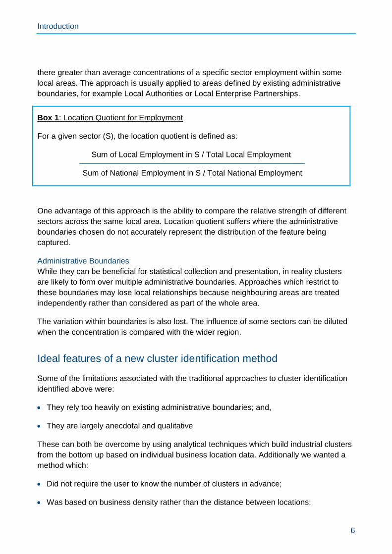
Box 1: Location Quotient for Employment

For a given sector (S), the location quotient is defined as:

Sum of Local Employment in S / Total Local Employment

Sum of National Employment in S / Total National Employment

One advantage of this approach is the ability to compare the relative strength of different

sectors across the same local area. Location quotient suffers where the administrative

boundaries chosen do not accurately represent the distribution of the feature being

captured.

Administrative Boundaries

While they can be beneficial for statistical collection and presentation, in reality clusters

are likely to form over multiple administrative boundaries. Approaches which restrict to

these boundaries may lose local relationships because neighbouring areas are treated

independently rather than considered as part of the whole area.

The variation within boundaries is also lost. The influence of some sectors can be diluted

when the concentration is compared with the wider region.

Ideal features of a new cluster identification method

Some of the limitations associated with the traditional approaches to cluster identification

identified above were:

They rely too heavily on existing administrative boundaries; and,

They are largely anecdotal and qualitative

These can both be overcome by using analytical techniques which build industrial clusters

from the bottom up based on individual business location data. Additionally we wanted a

method which:

Did not require the user to know the number of clusters in advance;

Was based on business density rather than the distance between locations;

Introduction

7

Did not force all locations into a cluster, i.e. had a robust approach to outliers;

Produced clusters which reflected the true shape of the area.

The algorithm Density-Based Spatial Clustering of Applications with Noise was identified

as the best solution.

Notes on the Data

8

Notes on the Data

Inter-Departmental Business Register

The main data source for this analysis was the Inter-Departmental Business Register

(IDBR). This is a comprehensive list of UK businesses registered for either Value Added

Tax (VAT) or Pay As You Earn (PAYE), produced by the Office for National Statistics

(ONS). The data is primarily used as a sampling frame for business surveys but is also

used for analysis of business activities.

The main sources of data for the IDBR are the Annual Business Survey, Business

Register and Employment Survey, VAT from HMRC (Customs) and PAYE from HMRC

(Revenue). Additional input comes from Companies House, Dun and Bradstreet and other

ONS business surveys.

The IDBR covers 2.6 million businesses across all sectors of the UK economy. These

account for around 97% of UK turnover. This includes 2.5 small businesses, including

some with no employees, however an additional estimated 3 million micro businesses not

registered for VAT or PAYE are not captured.

Further notes on the data can be found in the accompanying results as well as in Annex A.

BEIS access to the data

BEIS has received quarterly snapshots of the IDBR from 2007. This allows the department

to perform longitudinal analysis.

In accordance with BEIS’ data agreement with the ONS disclosure rules are applied to all

outputs which use the IDBR. This is to ensure that individual businesses cannot be

identified in the results. Figures in all the results tables are also rounded.

Likely date for the data

This project mainly used data from the 2015 (quarter 1) snapshot of the IDBR. We

consider this data refers to the state of businesses in 2014 due to time lags in collecting

and uploading the data. Throughout the report this will be referred to as ‘2015 data’ to

make it clear this was the IDBR snapshot used. The analysis also uses 2010 data from the

2010 (quarter 1) snapshot (likely to refer to 2009).

Features used for this analysis

The IDBR holds data for a number of different statistical units. This analysis is based on

information at local unit level which refers to individual business premises rather than an

Notes on the Data

9

enterprise’s headquarters. Businesses can have multiple local units if they have

employees in more than one location.

The main variables used in the analysis were postcode, SIC 2007 (Standard Industrial

Classification) and employment.

National Statistics Postcode Lookup (NSPL)

The NSPL is a database of location information associated with every postcode in the UK,

produced by the ONS (https://data.gov.uk/dataset/national-statistics-postcode-lookup-uk).

The NSPL was matched with data from the IDBR using the postcode associated with each

local unit. This process is known as geocoding and allowed the data points to be plotted

onto a map more precisely.

Map Templates

The map outlines for the UK and Local Enterprise Partnerships used in the results of this

analysis were obtained via the ONS Open Geography Portal

(http://geoportal.statistics.gov.uk).

Sector Selection

10

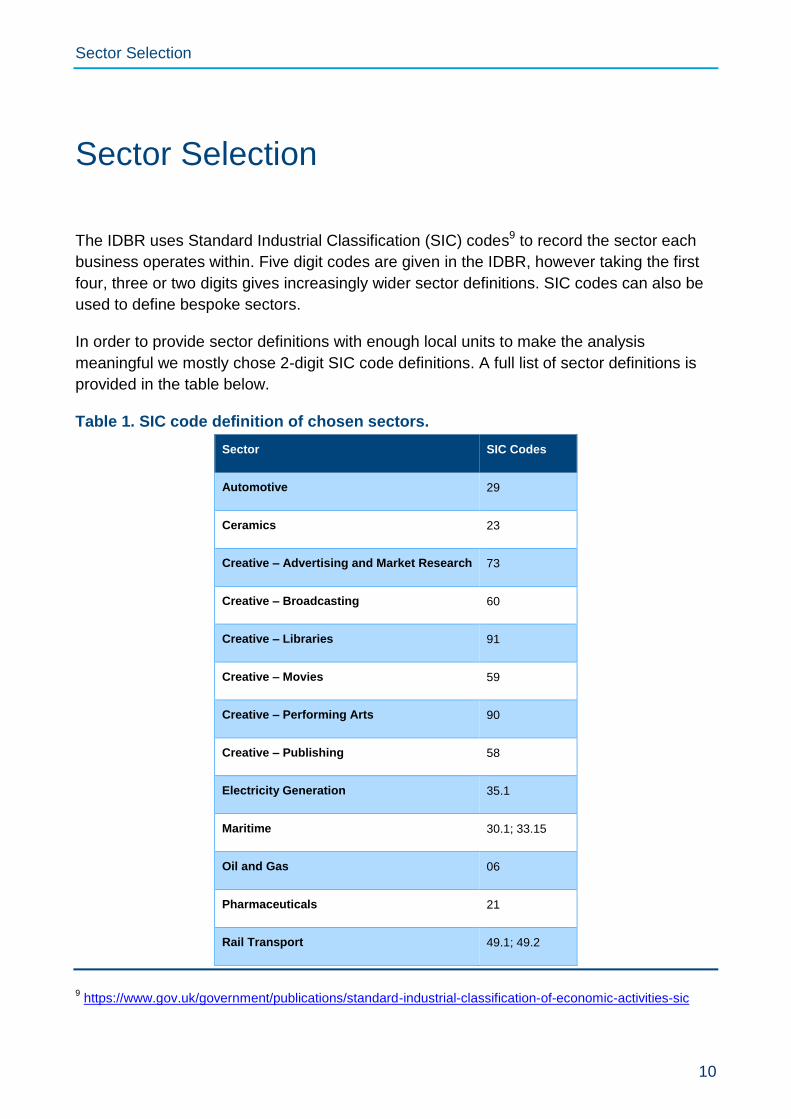
Sector Selection

The IDBR uses Standard Industrial Classification (SIC) codes9 to record the sector each

business operates within. Five digit codes are given in the IDBR, however taking the first

four, three or two digits gives increasingly wider sector definitions. SIC codes can also be

used to define bespoke sectors.

In order to provide sector definitions with enough local units to make the analysis

meaningful we mostly chose 2-digit SIC code definitions. A full list of sector definitions is

provided in the table below.

Table 1. SIC code definition of chosen sectors.

Sector SIC Codes

Automotive 29

Ceramics 23

Creative – Advertising and Market Research 73

Creative – Broadcasting 60

Creative – Libraries 91

Creative – Movies 59

Creative – Performing Arts 90

Creative – Publishing 58

Electricity Generation 35.1

Maritime 30.1; 33.15

Oil and Gas 06

Pharmaceuticals 21

Rail Transport 49.1; 49.2

9 https://www.gov.uk/government/publications/standard-industrial-classification-of-economic-activities-sic

Sector Selection

11

Robotics 28.22; 28.99

Steel and Iron 24.1; 24.2; 24.3

The list in Table 1 is broadly linked to industries within the Industrial Strategy Green

Paper10. This broad selection enabled the new analytical approach to the tested with

sectors of varying size and distribution across the UK.

10

https://www.gov.uk/government/uploads/system/uploads/attachment_data/file/611705/building-our-industrial-strategy-green-paper.pdf

Density-Based Spatial Clustering of Applications with Noise (DBSCAN)

12

Density-Based Spatial Clustering of Applications with Noise (DBSCAN)

Density-Based Spatial Clustering of Applications with Noise11 (DBSCAN) was the primary

technique used in this analysis. Hahsler and Pienkenbrock12 developed the

implementation we used. The methodology is outlined briefly below as well as the rationale

for using this approach.

Rationale

In order to overcome the limitations of previous cluster analysis (discussed above) the

chosen methodology needed to identify high concentrations of points without relying on

existing boundary definitions. DBSCAN uses locations of individual businesses to form

clusters from the bottom up. The results are areas which fall within and across

administrative boundaries.

Another advantage of DBSCAN over other methodologies is it does not restrict the shape

of the resulting clusters. Some algorithms force the points into areas defined by convex

boundaries which do not represent the natural growth of clusters.

The technique needed to be versatile to deal with a variety of sectors (outlined in the

section above). An important feature was that the user does not need to specify the

number of clusters in advance (as with k-means) as this restricts the results. Control over

the clusters in DBSCAN is based on two parameters which is a more flexible approach

(this is outlined in more detail below).

The final advantage of DBSCAN is that is has a robust approach to outliers, points which

are not clustered. Unlike some clustering algorithms DBSCAN does not force every point

into a cluster but allows points to be defined as ‘noise’ if they do not meet the density

requirements.

Limitations of the DBSCAN approach

As with any technique there are limitations. It is important to understand these when

looking at and interpreting the final results.

11

Ester et al. (1996) A density-based algorithm for discovering clusters in large spatial databases with noise.

12 Hahsler and Pienkenbrock. (2015) https://cran.r-project.org/web/packages/dbscan/vignettes/dbscan.pdf

Density-Based Spatial Clustering of Applications with Noise (DBSCAN)

13

The algorithm is not suitable for all sectors. Where there is a relatively even distribution of

businesses across the country spatial clusters are unlikely to form and the results will be

less meaningful. There are also problems with very large sectors as the technique requires

large amounts of computer memory.

This implementation of the algorithm calculates the distances between points as though

they lie on a flat surface. The Earth however is spherical therefore a certain level of

distortion will occur when the distances are projected onto the UK. A circle defined on a

flat surface will produce an oval area on a sphere. Given most areas defined are small this

is unlikely to impact on the results but is worth bearing in mind.

As previously mentioned the user has to select two inputs (parameters) in advance which

control the granularity of results and vary depending on the sector. The choice of these

parameters is not fixed and whilst there are a few ‘rules of thumb’ it is ultimately a

subjective decision. To ensure the same process was applied to all sectors a methodology

was developed to reduce the number of potential pairs of parameters.

In addition, one of the parameters is defined in terms of degrees latitude/longitude,

combined with the spatial distortion outlined above, this make this difficult to interpret.

Quality Assurance

The application of the DBSCAN technique to the IDBR data had not been used within the

department before. As well quality assurance of the code the results were combined with

another technique (Kernel Density Estimation – explained in the next section). This

allowed us to sense check the results by checking the two methods produced similar

outputs.

How the DBSCAN algorithm works

DBSCAN is a density based clustering algorithm, it looks for areas of highly concentrated

data points and highlights those groups which are ‘suitably’ dense – as defined by the

parameters. At the end of the algorithm every point will have been assigned to a cluster or

identified as noise. This can be mapped which allows further analysis to be performed.

Parameters

The parameters (inputs) the user provides to the DBSCAN algorithm have an impact on

the results. These will define the types (size, number) of cluster which are captured. The

two values required for the algorithm are a ‘radius’ and a ‘minimum density threshold’.

Density-Based Spatial Clustering of Applications with Noise (DBSCAN)

14

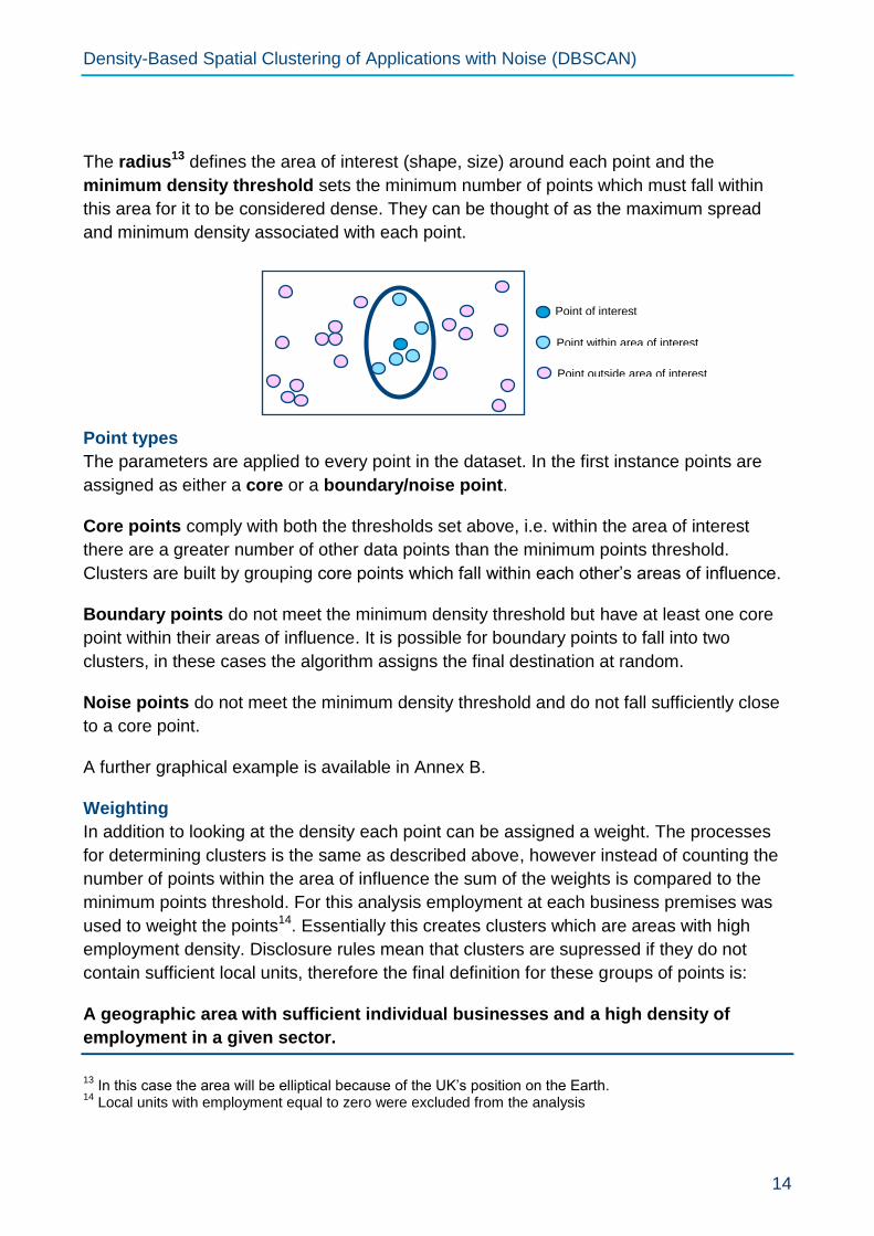
The radius13 defines the area of interest (shape, size) around each point and the

minimum density threshold sets the minimum number of points which must fall within

this area for it to be considered dense. They can be thought of as the maximum spread

and minimum density associated with each point.

Point types

The parameters are applied to every point in the dataset. In the first instance points are

assigned as either a core or a boundary/noise point.

Core points comply with both the thresholds set above, i.e. within the area of interest

there are a greater number of other data points than the minimum points threshold.

Clusters are built by grouping core points which fall within each other’s areas of influence.

Boundary points do not meet the minimum density threshold but have at least one core

point within their areas of influence. It is possible for boundary points to fall into two

clusters, in these cases the algorithm assigns the final destination at random.

Noise points do not meet the minimum density threshold and do not fall sufficiently close

to a core point.

A further graphical example is available in Annex B.

Weighting

In addition to looking at the density each point can be assigned a weight. The processes

for determining clusters is the same as described above, however instead of counting the

number of points within the area of influence the sum of the weights is compared to the

minimum points threshold. For this analysis employment at each business premises was

used to weight the points14. Essentially this creates clusters which are areas with high

employment density. Disclosure rules mean that clusters are supressed if they do not

contain sufficient local units, therefore the final definition for these groups of points is:

A geographic area with sufficient individual businesses and a high density of

employment in a given sector.

13

In this case the area will be elliptical because of the UK’s position on the Earth. 14

Local units with employment equal to zero were excluded from the analysis

Point within area of interest

Point outside area of interest

Point of interest

Density-Based Spatial Clustering of Applications with Noise (DBSCAN)

15

Final Presentation

Disclosure rules associated with the IDBR mean we are not able to show the location of

individual businesses on a map. The results therefore show outlines of the clusters.

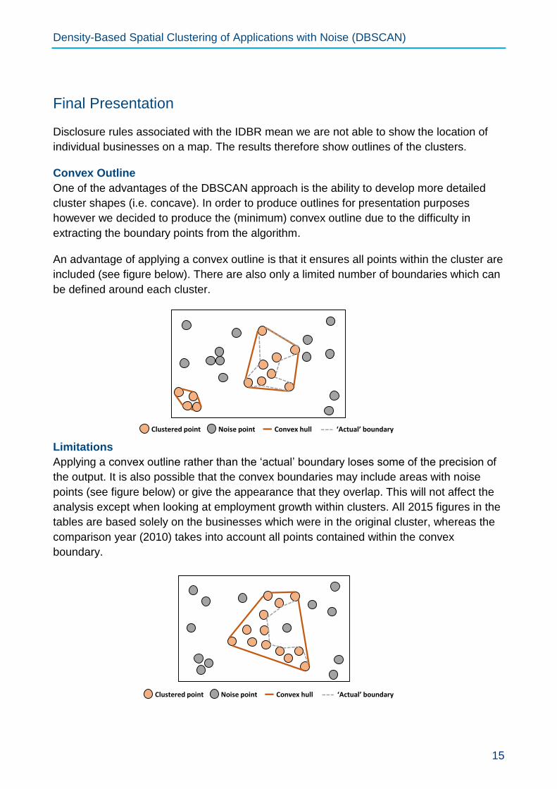
Convex Outline

One of the advantages of the DBSCAN approach is the ability to develop more detailed

cluster shapes (i.e. concave). In order to produce outlines for presentation purposes

however we decided to produce the (minimum) convex outline due to the difficulty in

extracting the boundary points from the algorithm.

An advantage of applying a convex outline is that it ensures all points within the cluster are

included (see figure below). There are also only a limited number of boundaries which can

be defined around each cluster.

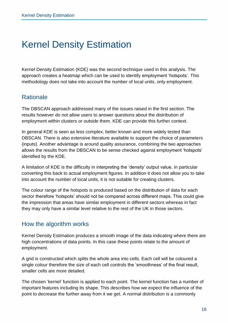
Limitations

Applying a convex outline rather than the ‘actual’ boundary loses some of the precision of

the output. It is also possible that the convex boundaries may include areas with noise

points (see figure below) or give the appearance that they overlap. This will not affect the

analysis except when looking at employment growth within clusters. All 2015 figures in the

tables are based solely on the businesses which were in the original cluster, whereas the

comparison year (2010) takes into account all points contained within the convex

boundary.

Clustered point Noise point Convex hull ‘Actual’ boundary

Clustered point Noise point Convex hull ‘Actual’ boundary

Kernel Density Estimation

16

Kernel Density Estimation

Kernel Density Estimation (KDE) was the second technique used in this analysis. The

approach creates a heatmap which can be used to identify employment ‘hotspots’. This

methodology does not take into account the number of local units, only employment.

Rationale

The DBSCAN approach addressed many of the issues raised in the first section. The

results however do not allow users to answer questions about the distribution of

employment within clusters or outside them. KDE can provide this further context.

In general KDE is seen as less complex, better known and more widely tested than

DBSCAN. There is also extensive literature available to support the choice of parameters

(inputs). Another advantage is around quality assurance, combining the two approaches

allows the results from the DBSCAN to be sense checked against employment ‘hotspots’

identified by the KDE.

A limitation of KDE is the difficulty in interpreting the ‘density’ output value, in particular

converting this back to actual employment figures. In addition it does not allow you to take

into account the number of local units, it is not suitable for creating clusters.

The colour range of the hotspots is produced based on the distribution of data for each

sector therefore ‘hotspots’ should not be compared across different maps. This could give

the impression that areas have similar employment in different sectors whereas in fact

they may only have a similar level relative to the rest of the UK in those sectors.

How the algorithm works

Kernel Density Estimation produces a smooth image of the data indicating where there are

high concentrations of data points. In this case these points relate to the amount of

employment.

A grid is constructed which splits the whole area into cells. Each cell will be coloured a

single colour therefore the size of each cell controls the ‘smoothness’ of the final result,

smaller cells are more detailed.

The chosen ‘kernel’ function is applied to each point. The kernel function has a number of

important features including its shape. This describes how we expect the influence of the

point to decrease the further away from it we get. A normal distribution is a commonly

Kernel Density Estimation

17

used kernel. Another important feature is the bandwidth which helps define the area

around each point that the kernel is applied to, similar to the radius parameter in DBSCAN.

This has a strong influence over the resulting estimate.

For each cell in the grid the kernel functions are combined to produce a density estimate

for that area. In this way KDE can also be used to interpolate values between the data

points.

Parameters used in this analysis

The description above outlines three of the parameters which are needed for the KDE:

kernel shape, bandwidth and grid size. In this analysis a square grid 750 cells high and

wide was applied to the outline of the UK to produce a smooth image.

The kernel function chosen was the normal distribution. The associated bandwidth for this

was selected based on a well supported rule-of-thumb according to the spread of the data.

Venables and Ripley15 offer a more detailed description on this and how this was first

implemented in R.

Colours

The colours on the final maps were assigned to cells based on their relative density

values, i.e. the highest density is associated with one end of the colour distribution and

lowest the other. The remainder of the range was split linearly.

The majority of the cells are not coloured because they do not contain any data points (for

example in areas of sea). There are also areas with much higher densities relative to the

remainder of the map. These values stretch the colour range and make it harder to see

finer details. A transformation was used which grouped the very high (and low) densities

together, these values were assigned a single colour which allows the user to detect

smaller changes in density.

This consolidated range meant high values were still marked but also ensured that the

whole colour distribution was used for the rest of the map.

15 Venables, W. N. and Ripley, B. D. (2002) Modern Applied Statistics with S. Springer, equation (5.5) on

page 130.

Findings

18

Findings

A full set of results from this analysis is available in the tables which accompany this report

however a guide to the output maps and some high level observations are set out below.

Map layout

Three different maps were produced for each sector in this analysis. These are explained

below along with the rationale for why they were produced. The examples in this section

are from the ‘Steel and Iron’ sector (SIC 24.1-3).

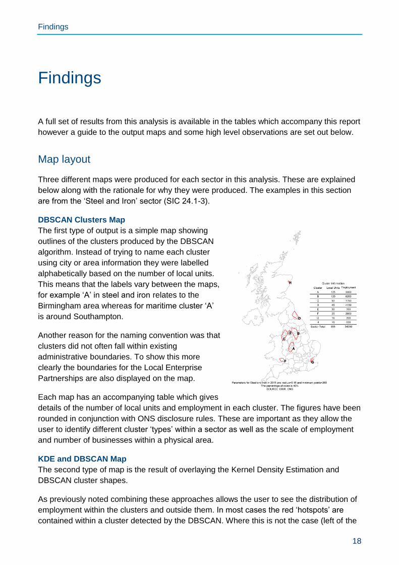
DBSCAN Clusters Map

The first type of output is a simple map showing

outlines of the clusters produced by the DBSCAN

algorithm. Instead of trying to name each cluster

using city or area information they were labelled

alphabetically based on the number of local units.

This means that the labels vary between the maps,

for example ‘A’ in steel and iron relates to the

Birmingham area whereas for maritime cluster ‘A’

is around Southampton.

Another reason for the naming convention was that

clusters did not often fall within existing

administrative boundaries. To show this more

clearly the boundaries for the Local Enterprise

Partnerships are also displayed on the map.

Each map has an accompanying table which gives

details of the number of local units and employment in each cluster. The figures have been

rounded in conjunction with ONS disclosure rules. These are important as they allow the

user to identify different cluster ‘types’ within a sector as well as the scale of employment

and number of businesses within a physical area.

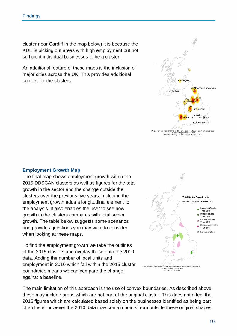
KDE and DBSCAN Map

The second type of map is the result of overlaying the Kernel Density Estimation and

DBSCAN cluster shapes.

As previously noted combining these approaches allows the user to see the distribution of

employment within the clusters and outside them. In most cases the red ‘hotspots’ are

contained within a cluster detected by the DBSCAN. Where this is not the case (left of the

Findings

19

cluster near Cardiff in the map below) it is because the

KDE is picking out areas with high employment but not

sufficient individual businesses to be a cluster.

An additional feature of these maps is the inclusion of

major cities across the UK. This provides additional

context for the clusters.

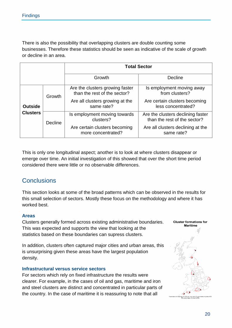
Employment Growth Map

The final map shows employment growth within the

2015 DBSCAN clusters as well as figures for the total

growth in the sector and the change outside the

clusters over the previous five years. Including the

employment growth adds a longitudinal element to

the analysis. It also enables the user to see how

growth in the clusters compares with total sector

growth. The table below suggests some scenarios

and provides questions you may want to consider

when looking at these maps.

To find the employment growth we take the outlines

of the 2015 clusters and overlay these onto the 2010

data. Adding the number of local units and

employment in 2010 which fall within the 2015 cluster

boundaries means we can compare the change

against a baseline.

The main limitation of this approach is the use of convex boundaries. As described above

these may include areas which are not part of the original cluster. This does not affect the

2015 figures which are calculated based solely on the businesses identified as being part

of a cluster however the 2010 data may contain points from outside these original shapes.

Findings

20

There is also the possibility that overlapping clusters are double counting some

businesses. Therefore these statistics should be seen as indicative of the scale of growth

or decline in an area.

Total Sector

Growth Decline

Outside

Clusters

Growth

Are the clusters growing faster than the rest of the sector?

Are all clusters growing at the same rate?

Is employment moving away from clusters?

Are certain clusters becoming less concentrated?

Decline

Is employment moving towards clusters?

Are certain clusters becoming more concentrated?

Are the clusters declining faster than the rest of the sector?

Are all clusters declining at the same rate?

This is only one longitudinal aspect; another is to look at where clusters disappear or

emerge over time. An initial investigation of this showed that over the short time period

considered there were little or no observable differences.

Conclusions

This section looks at some of the broad patterns which can be observed in the results for

this small selection of sectors. Mostly these focus on the methodology and where it has

worked best.

Areas

Clusters generally formed across existing administrative boundaries.

This was expected and supports the view that looking at the

statistics based on these boundaries can supress clusters.

In addition, clusters often captured major cities and urban areas, this

is unsurprising given these areas have the largest population

density.

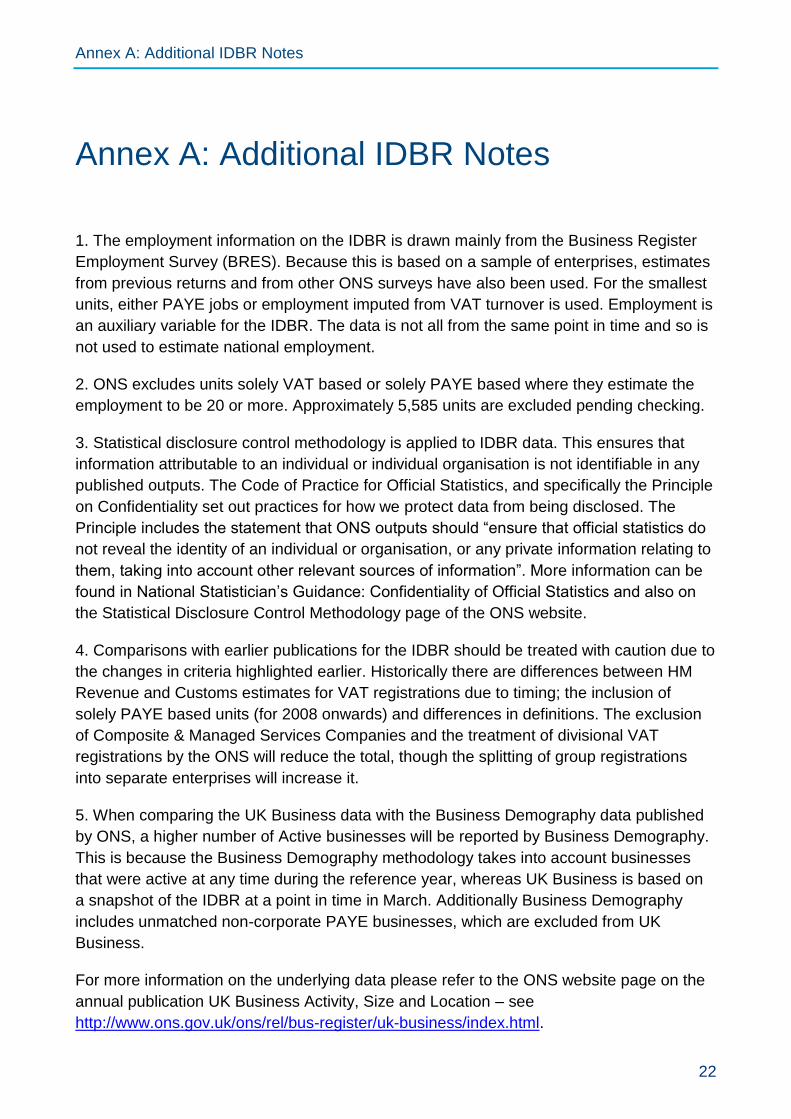
Infrastructural versus service sectors

For sectors which rely on fixed infrastructure the results were

clearer. For example, in the cases of oil and gas, maritime and iron

and steel clusters are distinct and concentrated in particular parts of

the country. In the case of maritime it is reassuring to note that all

Findings

21

the clusters are by the coast.

By contrast creative industries and service sectors, such as libraries and electricity

generation, are characterised by clusters covering a high proportion of the UK. In many

cases it appears that the algorithm is picking out urban areas. Arguably these are not

sectors which would be expected to cluster spatially however this does emphasise that this

method is more suited to specific sectors.

Types of cluster

Even in sectors where the results do not show definitive clusters it can be possible to

identify groups of similar areas in terms of local units and employment.

Annex A: Additional IDBR Notes

22

Annex A: Additional IDBR Notes

1. The employment information on the IDBR is drawn mainly from the Business Register

Employment Survey (BRES). Because this is based on a sample of enterprises, estimates

from previous returns and from other ONS surveys have also been used. For the smallest

units, either PAYE jobs or employment imputed from VAT turnover is used. Employment is

an auxiliary variable for the IDBR. The data is not all from the same point in time and so is

not used to estimate national employment.

2. ONS excludes units solely VAT based or solely PAYE based where they estimate the

employment to be 20 or more. Approximately 5,585 units are excluded pending checking.

3. Statistical disclosure control methodology is applied to IDBR data. This ensures that

information attributable to an individual or individual organisation is not identifiable in any

published outputs. The Code of Practice for Official Statistics, and specifically the Principle

on Confidentiality set out practices for how we protect data from being disclosed. The

Principle includes the statement that ONS outputs should “ensure that official statistics do

not reveal the identity of an individual or organisation, or any private information relating to

them, taking into account other relevant sources of information”. More information can be

found in National Statistician’s Guidance: Confidentiality of Official Statistics and also on

the Statistical Disclosure Control Methodology page of the ONS website.

4. Comparisons with earlier publications for the IDBR should be treated with caution due to

the changes in criteria highlighted earlier. Historically there are differences between HM

Revenue and Customs estimates for VAT registrations due to timing; the inclusion of

solely PAYE based units (for 2008 onwards) and differences in definitions. The exclusion

of Composite & Managed Services Companies and the treatment of divisional VAT

registrations by the ONS will reduce the total, though the splitting of group registrations

into separate enterprises will increase it.

5. When comparing the UK Business data with the Business Demography data published

by ONS, a higher number of Active businesses will be reported by Business Demography.

This is because the Business Demography methodology takes into account businesses

that were active at any time during the reference year, whereas UK Business is based on

a snapshot of the IDBR at a point in time in March. Additionally Business Demography

includes unmatched non-corporate PAYE businesses, which are excluded from UK

Business.

For more information on the underlying data please refer to the ONS website page on the

annual publication UK Business Activity, Size and Location – see

http://www.ons.gov.uk/ons/rel/bus-register/uk-business/index.html.

Annex B: Graphical Representation of DBSCAN

23

Annex B: Graphical Representation of DBSCAN

This builds on the section above describing how the DBSCAN algorithm works. The

example below shows an example where the minimum points threshold is four.

A and B are core points: Each has four or more other points within the area of influence

(including themselves)

C is a boundary point: It does not reach the minimum points threshold however it does

have a core point within its area of influence.

D and E are noise points: They do not reach the minimum points threshold and do not

have a core point within their area of influence.

The grey line shows the convex outline of the cluster. Point A and B are in the same

cluster because they fall within each other’s area of influence.