density dependence in time series observations of natural ...tds0009/articles/dennis and taper...
TRANSCRIPT

Density Dependence in Time Series Observations of Natural Populations:Estimation and Testing
Brian Dennis; Mark L. Taper
Ecological Monographs, Vol. 64, No. 2. (May, 1994), pp. 205-224.
Stable URL:
http://links.jstor.org/sici?sici=0012-9615%28199405%2964%3A2%3C205%3ADDITSO%3E2.0.CO%3B2-%23
Ecological Monographs is currently published by Ecological Society of America.
Your use of the JSTOR archive indicates your acceptance of JSTOR's Terms and Conditions of Use, available athttp://www.jstor.org/about/terms.html. JSTOR's Terms and Conditions of Use provides, in part, that unless you have obtainedprior permission, you may not download an entire issue of a journal or multiple copies of articles, and you may use content inthe JSTOR archive only for your personal, non-commercial use.
Please contact the publisher regarding any further use of this work. Publisher contact information may be obtained athttp://www.jstor.org/journals/esa.html.
Each copy of any part of a JSTOR transmission must contain the same copyright notice that appears on the screen or printedpage of such transmission.
JSTOR is an independent not-for-profit organization dedicated to and preserving a digital archive of scholarly journals. Formore information regarding JSTOR, please contact [email protected].
http://www.jstor.orgTue Jun 5 09:19:33 2007

Ecologlcai.Monogmphs.64(2), 1994. pp. 205-224 0 1994 by the Ecological Society of Amenca
DENSITY DEPENDENCE IN TIME SERIES OBSERVATIONS OF NATURAL POPULATIONS: ESTIMATION AND TESTING'
BIUAN DENNIS Department ofFish and l+.~ldlife Resources' and Department o f ,lrlathematics and Statistics.
C;nivers:tv ofldaho, Moscow, Idaho 83844 USA
MARK L. TAPER Department ofBlolog~: Montana State L'n~verslty, Bozeman, ,Wontuna 59717 LISA
Abstract. We report on a new statistical test for detecting density dependence in uni- variate time series observations of population abundances. The test is a likelihood ratio test based on a discrete time stochastic logistic model. The null hypothesis is that the population is undergoing stochastic exponential growth. stochastic exponential decline, or random walk. The distribution of the test statistic under both the null and alternate hy- potheses is obtained through parametric bootstrapping. We document the power of the test with extensive simulations and show how some previous tests in the literature for density dependence suffer from either excessive Type I or excessive Type I1 error. The new test appears robust against sampling or measurement error in the observations. In fact, under certain types of error the power of the new test is actually increased. Example analyses of elk (Cervus elaphus) and grizzly bear (CTrsus arctos horrihilis) data sets are provided. The model implies that density-dependent populations d o not have a point equilibrium. but rather reach a stochastic equilibrium (stationary distribution of population abundance). The model and associated statistical methods have potentially important applications in conservation biology.
Key words: bootstrapping; conservation hrolog~l;density dependence; elk; equilibrium; grizzlj~ hear; likelihood ratio; logistic model; nonlinear autoregressive model; population regulation; statistical power; stochastic dlference equation; stochast~c population model; time series analvsis.
and Reddingius 1989, Reddingius and den Boer 1989,
Whether or not populations in nature tend to have den Boer 1990, 199 I, Solow 1990, 199 1 , Turchin 1990,
growth rates regulated by their own densities has long Turchin et al. 199 1, Crowley 1992, Turchln and Taylor
been a key but frustrating problem of ecological re- 1992). One conceptual argument, exemplified by den
search (The Biological Laboratory 1957, McLaren 197 1. Boer (1 99 l) , asserts that if density dependence is to be
Colinvaux 1973, Kingsland 1985). It is widely ac- a cornerstone of ecological theory, a certain burden of
knowledged that possible answers to this question have proof needs to be satisfied. It is the role of density
broad theoretical implications for the structure of com- dependence theorists to demonstrate convincingly that
munities and the evolution of the species that comprise time series abundance data can be distinguished sta-
them (Pianka 1974. Cody and Diamond 1975, May tistically from the trajectories of a density-independent
1976, Roughgarden 1979. Emlen 1984, Diamond and stochastic growth model or even of a random walk
Case 1986). Moreover, assessment of density depen- model. Another argument discounts the need for sta-
dence has attained great practical importance in con- tistical detection of density dependence, claiming that
servation biology because the strength and form of population regulation is a purely logical consequence
density dependence have a large influence on the ex- of the ecological processes by which populations grow
pected survival times of natural populations (Ginzburg (Royama 1977, Berryman 1991a). A third argument
et al. 1990, Stacey and Taper 1992). questions the ecological meaning of existing statistical
The availability in recent years of "long term" ( ~ 2 0 methods for density dependence testing, because the
yr) data on population abundances has steered part of concept of a population equilibrium is unclear when
the dens~ty dependence controversy into a debate about the environment fluctuates (Wolda 1989). Throughout
statlstlcal concepts and methods (Eberhardt 1970, this conceptual debate, statistical methods for detecting
Reddlnglus 1971, 1990. Bulmer 1975, Royama 1977, density dependence have been introduced and refined
198 1, Slade 1977. V~ckery and Nudds 1984, 199 1, in a steady stream (Reddingius 197 1, Bulmer 1975,
Gaston and Lawton 1987, Pollardet al. 1987. den Boer Slade 1977, Vickery and Nudds 1984. Pollard et al. 1987, Reddingius and den Boer 1989, Turchin 1990,
Manuscript received 3 1 August 1992; revised 1 June 1993; den Boer 199 1). The conclusions of various data anal-
accepted 12 July 1993. ysis studies about the prevalence of density dependence Address reprint requests to the author at this department. seem to vary depending on which methods are used.
I
206 BRIAN DENNIS A h ID MARK L. TAPER Ecological Monographs
One group of studies has used a statistical model of population growth with a density dependence term proportional to the logarithm of population abundance (Reddingius 197 1, Bulmer 1975, Gaston and Lawton 1987, den Boer and Reddingius 1989, Reddingius and den Boer 1989, den Boer 1990, Vickery and Nudds 199 1, Crowley 1992). While different particular meth- ods for testing whether the density dependence term should be included in this model have different powers (Pollard et al. 1987. Vickery and Nudds 1991), these analyses frequently suggested that density dependence is not as prevalent as expected by ecological theory. The related concepts of "stabilization" (den Boer 1968, 1990) and "density vagueness" (Strong 19860, h) have been suggested to account for such findings; the con- cepts essentially take population growth to be density independent (but noisy) over a wide range of densities, with density dependent regulation occurring more or less sharply at very high densities.
However. in contrast to the above studies, Woiwod and Hanski (1992) and Holyoak and Lawton (1992) detected frequent density dependence using tests based on the same logarithmic density dependence model (among other tests). Woiwod and Hanski (1 992) ana- lyzed thousands of insect data sets, many of which exceeded 20 observations in length; Holyoak and Law- ton (1992) treated 32 insect data sets of 8 or 12 ob- servations. In these studies. longer time series showed increased prevalence of density dependence. Earlier re- sults of Hassell et al. (1989) and Solow and Steele (1990) had also highlighted the importance of sample size to the statistical power of density dependence tests.
Another set of studies employed a model with a density dependence term proportional to population abundance (Turchin 1990, Berryman 199 1a. Turchin et al. 199 1, Turchin and Taylor 1992). Woiwod and Hanski (1992) and Holyoak and Lawton (1992) used the model as well. These studies found widespread density dependence, sometimes in the form of delayed regulation (second order lags: see Turchin 1990). The statistical methods used to test whether the density dependence term(s) should be included in the model were based on standard results from ordinary regres- sion analysis. Generalization of these analyses to mul- tiple species systems has been reported (Berryman 199 1 b).
Still other analyses have been based on various sta- tistical properties of random walks (Vickery and Nudds 1984. den Boer 199 1, Crowley 1992). The studies re- garded a random walk model as the null hypothesis to be rejected by data according to some criterion. While Pollard et al. (1987) suggested that an exponential growth model (containing the random walk model as a special case) makes a more biologically interesting null hypothesis, the possibility that real data sets often cannot be distinguished from random walk trajectories remains unsettling to density dependence proponents. Indeed. den Boer (199 1) concludes that Nicholson's
Vol. 64, No. 2
(1933) hypothesis that populations "exist in a state of balance because densities fluctuate about a relatively stable norm" is not supported by random walk com- parisons or other statistical tests. Though den Boer (1991) does caution that these analyses do not mean that populations obey random walk models, his results should inspire some rereadings of Birch's (1957) and Andrewartha's (1 957) earlier density independence ar- guments.
In this paper, we introduce a new test for density dependence in time series data of population abun- dances. We propose that a discrete time stochastic lo- gistic model used by Turchin (1990) and Berryman (1 99 l a ) can serve as a useful and descriptive model for such testing in a variety of ecological situations. Statistical inference methods for this model, however. have not been well understood in the past. We develop parameter estimation methods and hypothesis testing methods for the model and focus on a likelihood ratio hypothesis test of density-independent vs. density-de- pendent population growth. Because the distribution of the test statistic is intractable, we show how its crit- ical values can be estimated with a parametric boot- strapping method. The power properties of this new test are documented here with extensive simulations. We illustrate the use of the test with examples. The results of past empirical studies are likely influenced by the statistical testing methods used. In particular, we show that the randomization test of Pollard et al. (1987) has low power (excessive Type I1 error) com- pared to the new test. Also. we find that the regression tests of Turchin (1 990) and Berryman (1 99 l a ) suffer from inflated size (excessive Type I error). The likeli- hood ratio test proposed here. by contrast, is a size 0.05 test and represents the practical limits of power that can be attained for the stochastic logistic growth model. We discuss the effects of sampling variability, the ecological interpretation of density dependence testing. the concept of a stochastic equilibrium, and the potential use of the new test in population viability analysis.
Let N, represent population abundance (as censused, estimated. or indexed) at time t , where t = 0. 1, 2, . . . . The model we present relates N,, , to N,:
Here a and h are constants, u is a positive constant, and aZ, is a random shock to the population growth rate. In thls paper. we are mostly concerned w ~ t h values of b such that b 5 0. We assume that Z, has a normal distribut~on w ~ t h a mean of 0 and a vanance of 1 [we wrlte 2, - normal(0, I)]. and that Z , , Z , , 2,. . . . are uncorrelated. The model lnvolves two essent~al Ideas. First, the per-unit-abundance growth rate 1s defined In dlscrete time as In N, , , - In N,, analogous to ( l l n ) dn/
Ma\ 1994 DENSITY DEPENDENCE 207
dt = d In n/dt in continuous time. Second, that rate so defined is taken to be a linear function of N, plus noise.
The constant b is the slope of the linear function. If b = 0, the per-unit-abundance growth rate does not depend on N,. When b < 0. the per-unit-abundance growth rate decreases as N, becomes larger. An increas- ing per-unit-abundance growth rate, or Allee effect. results when b > 0 (Dennis 1 9 8 9 ~ ) .
The type of variability inherent in the model (Eq. 1) is "environmental" as opposed to "demographic." Models with demographic variability become essen- tially deterministic as population size becomes large (see discussion by Dennis et al. 199 1). A population governed by Eq. I, however, fluctuates at large as well as small sizes. The distinctions between environmental and demographic variability have ramifications in con- servation biology (Leigh 198 1 , Shaffer 198 1, Goodman 1987, Simberloff 1988, Dennis et al. 1991. Wissel and Stocker 199 1).
The population abundances No. N,. N,, . . . are not independent under this model. even though the ran- dom shocks (Z,) are independent. As we show later in this paper, failure to account for the dependence among the N, values is the source of flaws in some previous statistical tests for density dependence. The stochastic process N, defined by Eq. 1 is a Markov process: given that the population has attained some particular size n, at time t, the future distribution of population sizes depends on n,, but not on past sizes.
The Markov property is a fairly general assumption applicable in many ecological situations. The deter- ministic analogue of the Markov property is simply that population abundance can be described by a first- order difference equation. Even in populations with overlapping generations or age structure, some index of population abundance can behave as if governed by a first-order difference equation. For example, Livdahl and Sugihara (1 984) and Barlow (1 992) document sys- tems in which complex, nonlinear life histories give rise to simple linear dependence of per-unit-abundance growth rate on abundance. Also. Cushing (1989) has provided a theoretical justification of how a simple nonlinear difference equation can emerge from a pop- ulation projection matrix model (such as a Leslie ma- trix) in which there is nonlinear dependence of de- mographic rates on population abundance. We discuss later the evaluation of the model for a given data set by residual analysis and by testing for second-order lags (see H~pothesis testing and Discussion).
We point out that the mean population abundance at time t + 1 under the model is not given by Eq. 1 with u = 0. Because E[exp(uZ,)] = exp(u2/2) and be-
time logistic model that has been analyzed extensively in population ecology (May 1976):
n,, , = n,exp(r + bn,). (3)
This model is known also as a Ricker equation from its similarity to the Ricker stock-recruitment relation- ship in fisheries (Ricker 1954). The linear form r + hn, is a simple way of representing density dependent feed- back in the per-unit-abundance growth rate (as defined
by In n,, , - In n,). The deterministic model has a positive point equilibrium at
ti = -r/b, (4)
provided b < 0. Eq. 3 may seem an overly simplified representation
of the complex processes of density dependence in nat- ural populations. However, the linear relationship r + hn, can be regarded as a Taylor series approximation near 2 of a more biologically detailed rate function (Dennis and Patil 1984, Dennis and Costantino 1988). The stability properties of ti and the dynamic behaviors of the deterministic model up to and including chaos are well known (May 1976). The growth model defined by Eq. 1 is a stochastic generalization of Eq. 3 and can be regarded as a type of stochastic, discrete time logistic model.
This stochastic logistic model becomes a first-order nonlinear autoregression model when transformed to a logarithmic scale. By letting X; = In N,. we obtain the following time series model from Eq. 1:
.Y,_, = X; + a + hP1 + uZ,. (5)
Transforming the model to a logarithmic scale has three main advantages. First. theoretical statistical knowledge about such nonlinear autoregressive models has increased in recent years (Tong 1990). Use of Eq. 5 provides connections between ecological time series data, mathematical population modeling, and estab- lished results in mathematical statistics. Second, valid point estimates (but not confidence intervals or hy- pothesis tests) of the parameters can be obtained with ordinary linear regression packages (see Parameter es-timation). Third, for some parameter values, one can obtain a diffusion process approximation to .Y,. Such an approximation provides simple expressions for long- run statistical properties of X,,including the stationary distribution and mean first-passage times (see Discus- sion).
The model can be altered to include second- or high- er order lags. The model would take the form
N,,, = N,exp(a + b , N , + b , N , , + . . .
cause of the Markov property, the mean population abundance at time t + 1 given N, = n, is
,,+ h,,,'Y+ I + UZ,) (6)
for incorporating time lags up to order m. Using this model. Turchin ( 1990) and Turchin et al. (1 99 1) have
E(N,+, IN, = n,) = tz,exp(r + bn,). (2) argued for the prevalence of second-order lags in eco- Here r = a + (u2/2). logical populations. We make some preliminary rec-
A deterministic analogue to Eq. 2 is a type of discrete ommendations in this paper (see Discussion) about how

208 BRIAN DENNIS A h ID MARK L. TAPER Ecological Monographs
testing for second-order lags might be accomplished. A full account of the statistical properties of Eq. 6 and of statistical inference methods for the model must be deferred to a future paper.
An alternative first-order population model was in- troduced by Reddingius (1 97 1):
Royama (1981) modified this model to incorporate higher order time lags. On a logarithmic scale, Eq. 7 becomes
where, as before, X., = In ,V,. A statistical motivation for use of this model is that it can be written in the form of a linear, first-order autoregressive model
(AR( 1)):
A',, , - jI = B ( x ; - jI) + a z , . (9)
with j~= - a l b and p = 1 + b. The AR(1) model has well-known statistical properties and established, packaged inference procedures. Written in the form of Eq. 7, the AR(1) model is seen to be a type of discrete time. stochastic Gompertz model [the Gompertz growth equation is (l/n)dn/dt = a + b In n]. While the statis- tical convenience of this model is a desirable quality, its biological postulate is that growth rate depends, if a t all, only logarithmically on population density. By contrast, the stochastic logistic model (Eq. I) structur- ally allows for stronger density dependence.
Computer-generating a time series from the sto-chastic logistic model using Eq. 5 is a simple procedure. Given numerical values of a , b, and a2, and starting at a fixed value .Yo = x,, one can easily calculate X I , X,, . . . recursively with the help of a routine for generating standard normal random variables. The simplicity of generating trajectories from the hypothesized stochas- tic mechanism underlying the data turns out to be a key for convenient and powerful statistical inferences (see Pararneter estimation and Hypothesis testing).
Distinguishing three cases of the model (Eq. 5) is important to density dependence testing. The cases form a series of three nested hypotheses. The simplest is Model 0:
If,: a = 0, b = 0. (1 0)
Model 0 defines X, as a discrete time Brownian motion process (or Wiener process) with zero drift (a = 0). This is the classic "random walk" model; X, has a normal distribution centered at s, with a variance of a2t. N o feedback of population density to the growth rate takes place (b = 0).
Model I is
Model I also defines X, as a discrete time Brownian motion process. but this time with a positive o r neg-
Vol. 64, No. 2
ative drift parameter (a i0). Under Model 1. X; has a normal distribution with a mean of .xu + a t and a variance of o.'t. Model 1 in the original population abundance scale (Eq. I) is a type of stochastic expo- nential growth or decay model. It is identical to the model described by Dennis et al. (1 99 1) for estimating extinction risks for endangered species (their parameter p is the same as a in this paper; a' is the same quantity in both papers). In Model 1, no density dependent feedback occurs (h = 0).
Finally, it is Model 2 that contains full-fledged den- sity dependence:
In many cases, a one-sided variant of Model 2 is of greatest interest. and we can redefine Model 2 as
Testing for density dependence can be regarded as de- termining whether the added parameter in Model 2 produces noticeably improved description of the data. The first step in such determination is estimating the unknown parameters from the data.
Statistically, the problem of connecting the model (Eq. 1) with data amounts to specifying a likelihood function. Let n,, n , , . . . ,n, be the recorded population abundances, so that q is the number of one-step tran- sitions and q + I is the total number of observations in the time series. Let x, = In n,>, x , = In n , , . . . , x, = In n, denote the log-transformed abundances. The likelihood function gives the probability that, under the stochastic mechanism defined by Eq. 1 , the out- come of the process N, would be the observed time series. The likelihood function is defined as the joint probability density function (pdf) for the random vari- ables Nu, N, , N,, . . . , N, evaluated at n,>, n , , n,, . . . , n,. It is more convenient to specify the likelihood func- tion for the log-transformed observations, because of the autoregressive structure indicated by Eq. 5. Given that log-population size is a t .u,-, a t time t - 1, the distribution of .Y, is, according to Eq. 5, normal with a mean of .u , , + a + b e x p ( x , ,) and a variance of a'. Thus, the pdf for .Y,, given X,+, = x,-,, is a normal curve:
Because of the Markov property, the joint likelihood of the data is the likelihood of a transition from x, to x,, multiplied by the likelihood of a transition from .I-, to .u2. etc. This joint likelihood is just a product of normal pdf s of the form given by Eq. 14. It is a function of the data values xu, x,, . . . , x,. and, more impor- tantly, of the unknown model parameters a, b, and a':
209 Ma1 1994 DENSITY DEPENDENCE
TABLE1. Maximb~m likelihood estimates for unknown parameter a,,' in Model 0 (random walk), parameters a , and a,' in Model 1 (stochastic exponential growth), and parameters h2 ,a?,and u2' in Model 2 (stochastic logistic growth). Observed population abuntiance at time t is n,: also x, = In n,, y, = s,- x, , . P = b,+ jl? + - . . + y,)/q, and A = (n,, + n , + . . . + n, l )/q.
Model 0
Model 1 a , = J t,'
4
2 CL,, - .P)(fl, I -
Model 2 h^, = " a,4
2 (n, I - A)' / I
This likelihood function L(a, h, a') plays a central role in parameter estumation and hypothesis testing.
We must note that Eq. 15, strictly speaking, is not the joint pdf of .Y,>. XI . . . . . X, evaluated at the ob- servations (it is not the full likelihood). Rather, it is the joint pdf of XI , X,. . . . , X,. conditional on .Yo =
.I-,, and evaluated at the observations. We recommend conditioning on the initial observed population size (and using Eq. 15 as the likelihood) because in practice the probabilistic mechanism producing the observa- tion ,u, is typically unknown.
Maximum likelihood (ML) parameter estimates have numerous desirable statistical properties (Stuart and Ord 199 1). ML estimates are defined as the parameter values, denoted a,6,and C', that jointly maximize L(a. h, a') (or equivalently, In L(a, b, a')). M L estimates are asymptotically efficient (they have the smallest vari- ances in large samples), are consistent (variances ap- proach zero as q + a ) . are asymptotically unbiased (biases approach zero as q + a ) , and have distribu- tions that approach normal distributions for large sam- ples. Standard mathematical statistics books only list these properties for independent, identically distrib- uted observations (Stuart and Ord 199 1. Rice 1988). We point out that these desirable properties of M L estimates have been demonstrated for time series mod- els (dependent data) of this type as well (Bhat 1974, Tong 1990).
Obtaining M L estimates for the random walk (Model 0) and exponential growth (Model 1) models is easy. Let L,>(a2) represent the likelihood function for Model 0. that is. Eq. 15 with a = 0 and h = 0. Let L,(a. u') represent the likelihood function for Model 1 (h = 0). Also. let J; = .u, - x, , , t = 1. 2, . . . , q. Note that J;
can be thought of as the per-unit-abundance growth rate observed in the population for transition t. The value of a'. denoted h,>', that maximizes L,(a2) appears in Table 1 . It is easily found by setting d In L,,(a2)/da' equal to zero and solving for a'. The values of a and u' that jointly maximize L , (a , a'), denoted a , and C I 2 . also appear in Table I. They are found by setting d In L,(a . ~ ' ) / a a and d In L , (a , a2)/da2 equal to zero si- multaneously.
The estimates for Models 0 and I are familiar ones. Let Y,, Y2, . . . , Y, denote the one-step differences in logarithmic population sizes: Y, = .Y, - .Y, , (the value realized by Y, in the data is J',). Because the Y,'s are increments of Brownian motion under Models 0 o r 1, much is known about their statistical properties (see Dennis et al. 199 1). Under Model 0, Y, - normal(0. a') and Y,, Y,. . . . , Y, are independent. Under Model I . Y, - normal(a, a') and Y,, Y2, . . . , Yq are indepen- dent. Both models reduce to simple cases of random sampling from normal distributions. Thus, standard confidence intervals from normal theory for u2 (Model 0) o r a and a 2 (Model I) are valid and exact. Dennis et al. (1991) give further details.
For the full stochastic logistic model (Model 2), ob- taining M L estimates is also easy. T o keep notation consistent, we will write L,(a, h. a2) instead of L(a, h. a') for the likelihood function of Model 2 (Eq. 15). The values of h, a , and u' that jointly maximize L,(a, h, a2) are listed in Table 1. The Model 2 estimates are also familiar ones. The estimates of a and hare least squares estimates obtained by performing a linear regression of J:, on n , ,, t = 1, 2, . . . , q. Thus. a,, h,. and C22 can be calculated with any standard regression package.
Confidence intervals printed by standard regression packages, however, are not valid for Model 2. Printed hypothesis tests for parameter values are not valid ei- ther. For the printed intervals and tests to be valid. the Y,'s would have to have independent normal(a + h n , ,, u2) distributions (the standard linear regression model). Under Model 2, though, the Y,'s are not independent. due to the autoregressive structure of the model, nor d o they have unconditional normal distributions. The

BRIAN DENNIS A N D MARK L. TAPER Ecological Monographs
overlap between the standard linear regression model and Model 2 stops at point estimation; both models happen to have identical ML estimates. The statistical distributions ofthe ML estimates under the two models are radically different. though, and so interval esti- mates and hypothesis tests for Model 2 cannot be based on the ordinary regression model.
Instead, approximate confidence intervals for pa- rameters in Model 2 can be found by either bootstrap- ping or jackknifing. Bootstrapping involves estimating the distributions of a,, h,, and CZ2in some fashion using the data. The following parametric bootstrap method makes efficient use of the information present in mod- est-sized samples (q = 20). The procedure is simple but requires some computer programming. First. from the data calculate the ML parameter estimates for Model 2 (Table 1). Second. repeatedly (say, 2000 times) com- puter-generate time series of the same length as the original data from the estimated model:
A given series generated from the estimated model ("bootstrapped" series) will be denoted with asterisks: s,>*, Each series should be started at the x,*, . . . ,s,*. observed initial value: .Yo = xu* = x,. To each such bootstrapped time series, fit Model 2 by calculating bootstrapped ML estimates, denoted a2*, 6,*.and CZ2*. using the expressions in Table 1. Third. for an ap-proximate 95% confidence interval for a, take the 2.5'h and the 97.5'h sample percentiles of the 2000 a,* val- ues. Likewise, use the h^?* and the C2'* values to con- struct confidence intervals for h and c2. An adjustment known as the bias-corrected percentile method (see Efron and Gong 1983) might make the coverage rate of the bootstrap confidence interval closer to 95%.
Jackknifing also involves using the data to estimate the distributions of i2.&?. and C2,, and it typically requires less computing time. Lele ( 1 99 1) describes a jackknifing technique for dependent data. For Model 2, Lele's technique entails dropping transitions from the data one by one and refitting the model each time to the remaining transitions. A transition here is a change in the data over one time step, that is, from x, , to x,. One performs the regressions on the pairs (v,,n,). (I>,, n,), . . . . (y,/, n,- ,). each time leaving out (y,. n, ,). where t = 1. 2. . . . , q. Lele (1 99 1) provides expressions for consistqnt estimates of the variances and covariances of a,, h,. and 5,'.
We have focused our computer simulations in this paper on evaluating hypothesis testing methods and cannot make any recommendations at this time con- cerning which type of confidence intervals for Model 2 parameters have superior properties. A large-scale evaluation of the coverage probabilities for boot-strapped and jackknifed confidence intervals is a topic for future research.
Missing data can be handled in the ML estimates by simply incorporating in the analysis all the one-step
Vol. 64, No. 2
transitions present in the data. Thus, if the jhyear (or whatever time period) population size, n!, was missing, one would perform the regression calculations using @I, no), Cb12> nl), . . . > @ / - I , n,-2), @,+,> n,+1), . . . >Cb1"?
n,-,). One missing year means that there are q - 2 one-step transitions present in the data (two transitions missing). The ML formulas (Table 1) would have q -2 instead of q as a divisor. and A (Table 1) would include n, , n , , . . . , nI - , , n,, ,, n,,,, . . . , n,-, in the sum (but not n , , or n,).
Statistical theory draws a careful distinction between a statistical hypothesis and a scientific hypothesis (for instance, see Stuart and Ord 199 1). A statistical hy- pothesis is an assumption about the form of a proba- bility model, and a statistical hypothesis test is the use of data to make a decision between two probability models. A scientific hypothesis, on the other hand, is an explanatory assertion about some aspect of nature.
For density dependence studies, a general scientific hypothesis of interest is the assertion that a popula- tion's abundance produces a negative feedback effect on its growth rate (Berryman 1991a). From this as- sertion, we expect that time series observations of a density-dependent population would lead us to favor Model 2 over Model 1 as a model of the population's abundance. However, investigators should be aware that other stochastic mechanisms besides ecological feedback can produce observations that pass statistical density dependence tests, including the test described here (see Discussion).
When deciding between two models. the likelihood ratio (LR) test originating with Neyman and Pearson provides the benchmark for test power (Neyman and Pearson 1933. Stuart and Ord 199 1). If the two prob- ability models are completely specified (no unknown parameters), the LR test has power greater than or equal to any other size cutest, according to the Neyman- Pearson Lemma (Stuart and Ord 199 1). Here, how- ever. Models 0, l , and 2 are not completely specified, that is, they contain unknown parameters. LR tests that are modified to accommodate unknown param- eters are sometimes called "generalized LR tests." The statistical criteria for choosing test methods are more complex when one or more of the models is not com- pletely specified. In some simple textbook cases (for example, a one-sided t test), the LR test is the uniformly most powerful test. In other cases, the power of the LR test tends to compare quite favorably to other tests according to various definitions of "asymptotic relative efficiency" (these criteria are reviewed by Serfling 1980 and Stuart and Ord 1991). Thus, LR tests for com- paring Models 0 and I , Models 1 and 2, or Models 0 and 2, if feasible to construct, would likely offer desir- able power properties.
In general, the LR test for comparing two models, i and J say, is constructed as follows. The model with
Ma\ 1994 DENSITY DEPENDENCE
the smallest number of unknown parameters typically forms the null hypothesis, while the more ~ o m p l e x model becomes the alternate hypothesis. Let L, denote the likelihood function for the null hypothesis (Model i ) , evaluated at the M L estimates of all unknown pa- rameters in the model. Essentially, L, represents the estimated joint probability density of the data (or es- timated likelinood that the data would have arisen) under Model i. Likewise, let L, denote the alternate hypothesis (Model J ) likelihood function. maximized over all parameter values permissible in the model. The LR test is to choose between Model i and Model j on the basis of the value of the LR test statistic:
The decision is made in favor of Model i if A,, > c, where c is some constant cutoff point selected by the investigator and is made in favor of Model J if A,, 5
c. The value of c is selected so that the probability of wrongly choosing Model J when the data in fact arise from Model i (that is, the probability of a Type I error) is fixed at some small number, a (the size of the test). The study of such LR tests occupies a prominent por- tion of any mathematical statistics text (e.g., Bain and Englehardt 1987, Rice 1988).
The essential problem in constructing an LR test is finding the value of c corresponding to the desired test size, a. In the normal-based linear models of analysis of variance and regression. the test statistic A,, is a monotone function of the more familiar variance ratio statistic. Under the null hypothesis, the variance ratio statistic has an F'distribution. The value of c then is calculated by transforming the 100(1 a)Ihpercentile-
of the appropriate Fdistribution. In a broad class of other models, including many nonlinear regression models. time series models, and loglinear models, the statistic G,,' = -2 In .I,,has, under the null hypothesis, a distribution that converges to a chi-square distri- bution as sample sizes increase. The value of c is ob- tained (approximately) from the 100( 1 percentile-
of the chi-square distribution. Unfortunately, for test- ing among Models 0, I , and 2, blind application of these traditional results can lead to erroneous infer- ences.
In the case of testing Model 0 (random walk) vs. Model I (exponential growth), the LR statistic does reduce to a statistic with an F distribution (with I and q - 1 degrees of freedom), o r equivalently, a Student's t distribution (q - 1 degrees of freedom). Under Model 0. L, = L,(CUL) is the likelihood function evaluated at the ML estimate of oL (Table I), and L, = L l ( a l , C12) is the likelihood function evaluated at the M L esti- mates of a and oL (Table 1). The LR test statistic can be written in several algebraically equivalent forms:
Here,
is the familiar t statistic for testing whether the mean is zero or not for independent normal(a, a2) random variables. Under Model 0, T,, has a Student's t dis-tribution with q - 1 degrees of freedom. Alternatively, TUl2= F,, has a n F distribution with 1 and q - 1 degrees of freedom. Thus, the cutoff point c for A,, is a simple function of an F or a Student's t percentile. Model 1 is favored over Model 0 if / T,, ( r where I,,,: is the 100[1 - (a/2)lth percentile of the appropriate Student's t distribution.
In some circumstances, a one-sided hypothesis about a might be of interest. For instance, a test of M,: a =
0 vs. I I , : a < 0 could be used to determine if an en- dangered species is in decline or not, provided the spe- cies is not abundant enough for density dependence effects to be important. The one-sided test in this case would reject H, if T,, 5 t ,-,,.
Unfortunately, for testing Model I vs. Model 2, the distribution of the LR statistic is unknown. The like- lihood function maximized under Model 2 (Eq. 15) is given by L2 = Lz(a7, b2, CL2). The LR test statistic can be written in the following forms:
Here G I z 2 = 2 In ,l,,, and
4
TI, = L[(q - 2) ( n , - ) 2 / ( q 7 7 ) ] 1. (21) I I
The statistic TI , is identical to the familiar t statistic used for testing whether the slope parameter is nonzero in a linear regression. However, TI , (Eq. 21) does not have a Student's t distribution, not even approximate- ly, due to the time dependence of the observations. Testing for density dependence based on an assumed Student's t distribution for T I , produces unacceptably inflated Type I error rates (see Discussion).
One should not even be lulled into using the tradi- tional chi-square approximation for the distribution of GlL2. Under the exponential growth model of the null hypothesis. the population is not ergodic (A',does not probabilistically tend to return to any given abundance level). The value h = 0 is at the edge of the set of values (h < 0) for which the stochastic process A: is ergodic. Without ergodicity, the theorems of mathematical sta- tistics that give the chi-square approximation for GI,? d o not apply. Simulations (not reported here) indicated that the use of the chi-square approximation produces inflated Type I error rates. As can be seen from Eq. 9, the situation is akin to testing whether (3 = 1 in an AR(1) process, a well-known case in which the chi- square approximation for Gtl2 fails (Dickey and Fuller 1981).
2 12 BRIAN DENNIS A h ID M A R K L. TAPER E:cological Monographs
Instead, the distribution of A,, (or T I ? , o r GIZ2) can be estimated from the data through parametric boot- strapping. The critical percentile. c, is an unknown function of the two unknown parameters. a and 02,in the null hypothesis (Model 1). If Model I did indeed give rise to the data, then the M L estimates (Table I) are in principle quite good estimates of a and u2. In fact, the ML estimate a , and the bias-corrected esti- mate of oZ given by
are the uniformly minimum variance unbiased esti- mates. We would expect therefore that the time series model given by
where Z,,%,. . . . are independent normal(0, I) random variables. represents a reasonably good estimate of the mechanism that produced the data under the null hy- pothesis. We have found in our simulations a slight but detectable advantage to using the unbiased esti- mate, C12. in place of C I L(see Test validation).
The bootstrap idea is straightforward. Generate data sets repeatedly from the cstinzatcdnull hypothesis model (Eq. 23). For each of these "bootstrap" data sets, fit Models 1 and 2 and calculate an LR statistic (A , , , TI,, or GIzL). The resulting 2000 or so LR statistic values constitute a random sample from the cstinzatcd dis- tribution of the test statistic under the null hypothesis. The appropriate sample percentile of those values be- comes the estimated critical value for the test. We use the term "parametric bootstrap test" instead of "Mon- te Carlo test" to emphasize the fact that the model under H I is being estimated (Beran 1986, Efron 1986). The terminology is common in the statistics literature (e.g., Schork 1992).
The parametric bootstrap likelihood ratio (PBLR) test is quite simple to conduct using the following steps. The two-sided test of H I : b = 0 vs. H,: h # 0 is de- scribed first. (I ) Obtain M L estimates for all parameters in Models 1 and 2 using the expressions in Table 1. (2) Calculate TI,' (or G I z 2 . o r A,,) as in Eq. 21. (3) Generate 2000 or more data sets in the form xu*,x,*. . . . ,xq* from the estimated null model (Eq. 23). Each of these bootstrap data sets should start at x,* = x, and be the same length as the original set. (4) Calculate for each bootstrap data set the parameter estimatesfor Models 1 and 2 (Table I), obtaining a , * , t I 2 * , a,*, b2*, CZ2*. (5) Obtain in this fashion 2000 (or so) bootstrap values of the LR test statistic, (Eq. 21; or ,1,,* or GILL*).Each of these TIL2* values represents an inde- pendent observation from the estitnatcd distribution of T I z Z (likewise AIL: GIZ2). (6) Take the 100(1 - u)lh sample percentile, .f<:.as the estimate of the critical percentile of the distribution of TILL. (7) Reject H I : b = 0 in favor of H,: b # 0 if the original value of TI,' is greater than .f,.
Alternatively, a t step 6 one can estimate a P value
Vol. 64. No. 2
for the test with the proportion of TIL2* values that are greater than or equal to T lL2 . The null hypothesis would be rejected if 5 cu. where P is the estimated P value.
Note that in each bootstrap cycle of the calculations, only the value of the original data, the original ML estimates, and the original test statistic need to be retained; the values a ,*. 6,*, tLL*, and x,*. a?*, ElL*,
.u,*,. . . ,x,* d o not need to be stored. The procedure is easily programmed and is acceptably fast: our pro- gram, written in the GAUSS matrix language (Aptech Systems 199 I), completes the calculations. using 8000 bootstrap samples, for one moderately sized (q - 16) data set in - 1 1 min on an old IBM AT/286. (A short SAS program written by the authors for conducting the PBLR test takes z 6 0 min to run on a 286 machine.)
The one-sided PBLR test of H I : A = 0 vs. H L : b < 0 is straightforward. In step 1 above, reject HLoutright if d, r 0; otherwise continue. In step 5 above, calculate TI,* using Eq. 2 1 for each of the bootstrap samples, instead of TIz2*. In step 6, estimate the critical per- centile of the distribution of T I L with the 100aih sample percentile, f , , , , of the T I ? * values. Alternatively, es- timate a P value by the proportion of TI?* values that are less than TI,. In step 7. reject H , if TI , 5 f l ,,. or if < a .
We point out that the distribution of TI, is not sym- metric, nor is it centered at zero. The two-sided test conducted with the 100(~u/2)'~ 100[1and - (a/2)lth sample percentiles of the TI,* values is different from the previously described two-sided test that uses the 100(1 a)lh percentile of the TI,'* values. The power -
properties of both tests have not been compared. A PBLR test of Model 0 against Model 2 might be
of interest in some studies. Other methods for distin- guishing a drift-free random walk from a density-de- pendent process (e.g., den Boer 1991) are likely not as powerful. The one-sided test of H,: (I = 0. b = 0 vs. H L : a # 0. b < 0 would be conducted as follows. (1) Obtain M L estimates for all parameters in Models 0 and 2 using Table 1. Reject H, outright if I;? r 0; otherwise continue. (2) Calculate the LR statistic as
(3) Generate bootstrap data sets in the form xu*,x,*, . . . ,s,* from the estimated random walk model,
starting at so*= xcj.(4) For each bootstrap data set, calculate the parameter estimates for Models 0 and 2: c,2* , a,*, LL*. t z2* . From these parameter estimates,
calculate a value of the LR statistic as
(5) Obtain in this fashion 2000 (or so) values of ,lOL*.
Ma) 1994 DENSITY DEPENDENCE 2 13
The provision of setting ,I,,* equal to 1 when b,* r 0 will result in a one-sided test. (6) Take the I 0 0 d h per- centile, i,,.as the estimate of the critical percentile of ,1,,. Alternatively. estimate a P value by the proportion of ,lo,* values that are less than 'IOL.(7) Reject H , if 'IOLi Xcr. or if P < LY.
Of course, Model 1 contains Model 0 as a special case. The pre\ iously described test of Model 1 against Model 2 thus implicitly includes Model 0 in the null hypothesis. Normally, the test of Model 1 against Mod- el 2 should be used, unless there are specific reasons for restricting the null hypothesis to a pure random walk.
The PBLR tests can accommodate missing data. The fundamental "observation" in the likelihood function (Eq. 15) is not a (logarithmic) population size, s,,but a transition from s, , to x,. If x, is missing from the data. it means that two transitions are missing: x , , to s,,and s,to s,,, . The likelihood function (Eq. 15) with p(x, Ixu, ,) and p(x,+, Ix,) omitted from the product is the joint pdf of X I , X,. . . . , X, , given s, and Xi+L, X,,,,. . . , X, given x i + , . This likelihood is used as the fundamental building block for parameter estimates and hypothesis tests.
When observations are missing, the M L parameter estimates for Model 2 are easiest to calculate with a least squares approach. The formulae (Table I) oth- erwise must be altered in messy ways. Take as the fundamental data set the logarithmic differences y,, y,, . . . , J ~ , , v , ~ ~ , J ~ + ~ ,. . . ,J ' ,(J\ ,J '~,, missing). Thesam- ple mean of the y12 values provides the ML estimate of a' for Model 0. The sample mean of the differences. 7,and the sample mean of the (y, p)2 values provide -
respectively the M L estimates of a and a 2 for Model 1 . The linear regression of y, on n , , (using all transi- tions present in the data) provides M L estimates of a and h for Model 2. The M L estimate for u2 in Model 2 would be the sum of squared errors (from the re- gression) divided by the number of transitions present (q - 2, if just one population size is missing). The bootstrap data sets are generated (Eq. 23 or 25) as a series of one-step transitions starting at xu (xu, XI*, X,*. . . . , X, ,*), followed by a series starting at s,,, (s,,,, Xi+,*, . . . , X,*). All parameter estimates and tests are thus conditioned on the observed starting val- ues, x, and x i + , , of series of one-step transitions.
An alternative approach to testing with missing data is to condition only on xu. Parameter estimates and the test statistic are computed as described above using all one-step transitions present in the data. However. bootstrap data sets are generated starting at xufor all times (xu, XI*, X2*. . . . ,X,*), including missing times. The bootstrap values of the test statistic are then cal- culated after omitting from the bootstrap data sets the generated observations occurring at missing times (that is, omit XI* before calculating TI,*).
The two approaches to handling missing data are subtly different. The first treats the uninterrupted time
series essentially as separate series, but assumes the series are governed by the same (density-independent o r -dependent) model. The first approach would be preferred if, for instance, the population was restarted at size x,, , after some drastic change (a harvest o r catastrophe). The second approach treats the uninter- rupted series as one single series with some observa- tions (the missing ones) simply unknown. Which ap- proach is most appropriate will be case specific, although the resulting tests are not likely to differ much unless the number of missing transitions is large. The statis- tical properties of the two approaches have not yet been compared.
Because the PBLR test is a parametric test. some additional model checking is advised in any applica- tion. Judicious use of model diagnostic techniques will help minimize problems associated with "Type 111 er- ror" (fitting the wrong model). In particular, serious departures of the data from the Markov property o r from the model could likely be detected through some form of residual analysis. For the stochastic logistic model, diagnostic techniques would center around the conditional residuals: P, = x, - x , , - a - b e x p ( x , ,), t = 1, 2, . . . , q. Under the model assumptions, these residuals should be approximately normal white noise. The residuals can be subjected to the customary anal- ysis techniques of linear time series modeling (see Tong 1990:322 for discussion). We often use the Lin-Mu- dholkar test for normality against asymmetric alter- natives (Lin and Mudholkar 1980, Tong 1990:324) in addition to the standard normal plots and autocorre- lation tests. There is a caveat, however: in the nonlinear setting, the adequacy of the normal-white noise ap- proximation is unknown and varies from model to model. The properties of these diagnostic techniques for the stochastic logistic model would be a worthwhile topic for future study.
According to statistical principles of asymptotic rel- ative efficiency, the PBLR tests represent approximate size (Y tests having power functions that cannot be ex- ceeded by much. The principles rest on large-sample theorems of statistics (Serfling 1980). But d o these as- ymptotic assurances apply to the data sets of moderate lengths likely to be encountered in ecological practice? A large-scale, Monte Carlo power assessment of the PBLR test of Model 1 against Model 2, along with comparative studies of other available tests, provides some answers.
It is desirable that statistical tests have several prop- erties. First. their size should be close to their nominal size, that is, i f the null hypothesis is true the probability of rejecting the null hypothesis should be close to what the investigator thinks it is. Second, the test should be powerful enough to detect scientifically interesting de- viations from the null hypothesis. Third, the test should be robust to measurement error. This last property is

2 14 BRIAN DENNIS A N D MARK L TAPER Ecolog~calMonographs Vol 64. No 2
1 . 0 0 0 7 ----- ranged from 4 to 64. In all. 64 d~fferentsets of ~ a r a m -
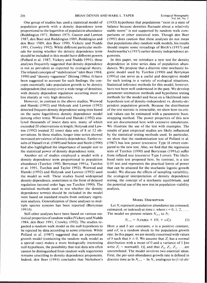
FIG. 1. A contour plot showing estimated power of the parametric bootstrap likelihood ratio test of density depen-dence as a function of model parameters a and b. The null hypothesis for the test is Model 1 (b = O), and the alternate hipothesis is Model 2 (h < 0). Each indicates location of 1000 simulated tests; each test used 200 bootstrap samples and the values q = 19, n,, = - a h , and c = 0.2. The power surface was estimated using a distance weighted least squares algorithm (McLain 1974).
particularly important when dealing with population abundance data, which commonly contain substantial uncertainty.
We have investigated the qualities of the PBLR test of Model 1 against Model 2 (both one- and two-sided) with Monte Carlo simulation. Using a known set of parameters we generate a time series of simulated pop-ulation densities according to Eq. 1. This simulated time series is then subjected to the PBLR test exactly as if it were data from field observations. For each set of parameters (a, b, u, q, and no: we have couched the simulations in terms of a rather than u2) chosen for study, this process was repeated a large number of times, usually 1000. All tests were conducted a t a nom-iaal 0.05 level. The proportion of times the null hy-pothesis was rejected was recorded for each parameter set. If the parameter h was zero, that is if the null hypothesis of no density dependence was true, this proportion represents a n estimate of the size of the test. If b was not zero then the proportion of rejections is an estimate of the power of the test under the set of parameters. We denote by $(a, b, u, q, nu) the proba-bility of rejection of the null hypothesis as a function of model parameters (power function), and by 4(a, b, u, y, no) its estimate from simulations.
Tcst size
We examined the size of the PBLR test (one- and two-sided) under a broad range of parameters. The parameters a and a ranged from 0.05 to 1.5, while q
-eters were tested each with two separate simulations of 1000 trials. The sample mean of these 128 values of 4 for the one-sided tests was 0.0504 with a sample variance of 0.0000470. The underlying population mean of the 4 values is thus not significantly different from 0.05 (Z = 0.66, A' = 128, P = .25). The sample variance was close to the variance expected under bi-nomial sampling, 0.0000475 (= 0.05(0.95)/1000). Fur-ther, despite the wide variety of parameters used. the distribution of 4 values observed was not significantly different from a normal distribution with a mean and variance of 0.05 and 0.0000475, according to a Kol-mogorov-Smirnov test (D = 0.06 1 1, N = 128, P > .5). Results for the two-sided tests (based on T,,2) were similar. Thus there is no reason to believe that the true size of the PBLR test is different from its nominal size. If any deviations d o exist, they are of insignificant mag-nitude.
The size results reported above were obtained for the PBLR test that uses the unbiased estimate, SI2 . instead of the M L estimate, Z12,in the estimated null hypothesis model (Eq. 23). We detected through sim-ulations a slight but noticeable increase in the test size over the nominal size of 0.05 when the M L estimate is used. While the increase is small enough to be of little practical importance, it is easily corrected simply by using S ,2 .
Tcst power
As with the size of the test, we investigated power extensively with simulations. The power of a test de-pends in general on the specific true values of the pa-rameters. We have assessed the influence of b, a , a, q, and nu on power. A number of our results contradict unreflective intuition.
First, the probability, $(a, b, u, q, nu), of rejecting the null hypothesis is nearly independent of the pa-rameter b as long as b is not zero (Fig. l). Thus, the influence of b on power is not continuous; instead, h acts as a switch to change the qualitative behavior of the model. This discontinuity in the power function is, from the standpoint of statistical theory, unusual (e.g., Bain and Engelhardt 1987:373). One would normally expect the power function to increase smoothly, start-ing from a level of a, as the parameter in question becomes farther from its hypothesized null value.
However, such smooth textbook dependence of power on b would in fact be a n undesirable property. The parameter b is related to the level around which X, is fluctuating according to the density-dependent model (Eq. 1). While the concept of point equilibrium (carrying capacity) is of questionable meaning in a sto-chastic model (Dennis and Costantino 1988, Wolda 1989), we can see that the level - a l b (Eq. 5) represents a center for the return tendencies of A',. If A', > a l h , then In A',, , is expected to decrease (Eq. 5), while if X, < a / b , In A:+, is expected to increase. One presum-
215
2 4 8 16 32 64 1 2 8 2 ; ~
"0
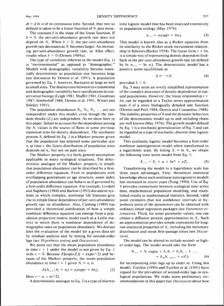
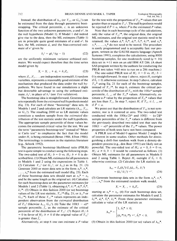
FIG 2 Estimated power of the parametnc bootstrap I~ke- l~hoodratlo test of dens~ty dependence as a funct~on of ~ n ~ t ~ a l
Ma) 1994
i . 0 ~- a u u
O.ol -L 1 I
DENSITY DEPENDENCE
,F the population density to move toward a central value
when displaced from it. It makes sense that a deviation in the initial population size would increase the test power. However, if the parameter a is low, then power decreases again if no is too far below the value of -a lh (Fig. 2b). With a low a and a low initial size, the pop- ulation will tend to increase for a number of time steps, making it difficult to distinguish the time series from one that would be produced by a population under- going exponential growth.
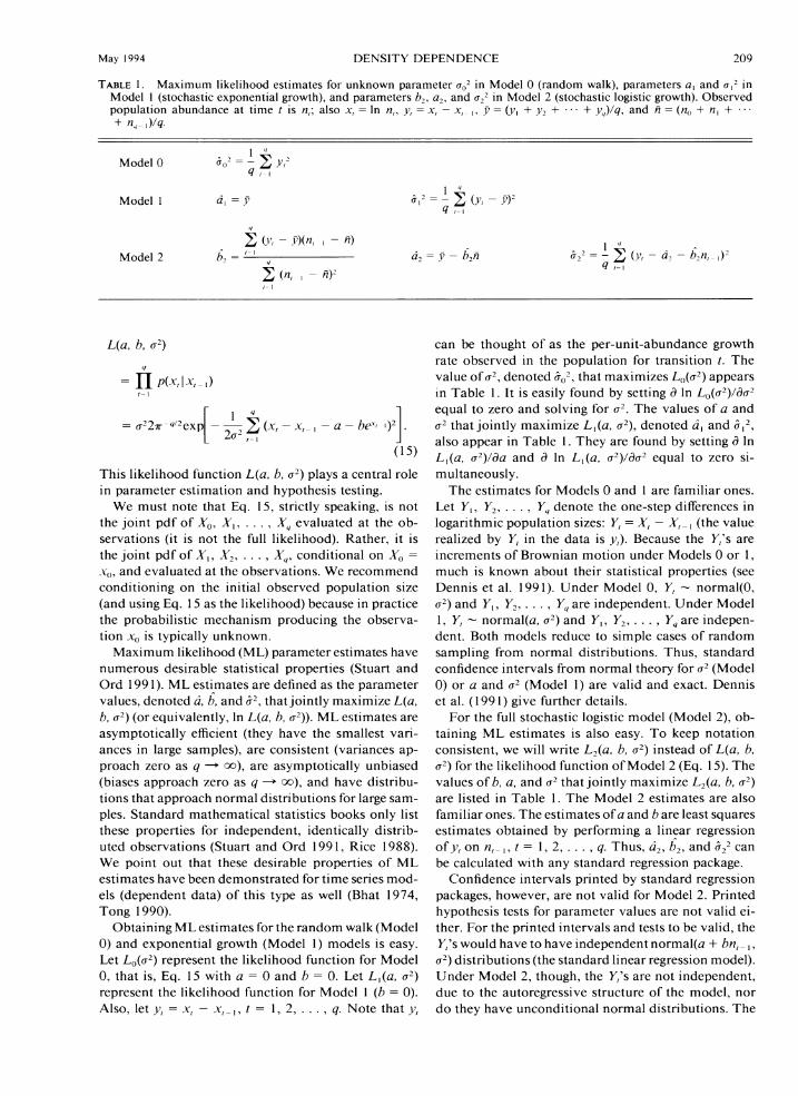
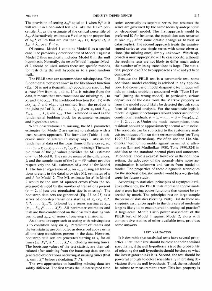
We turn now to the effect of environmental variation in growth rate on the power of the PBLR test. The parameter that measures environmental variation is o, the standard deviation of Y,= In (.V,/.Vl ,) conditional on A', , = n, ,. (The standard deviation of Y, condi-tional on hri,= n, is an unknown, increasing function o f o that depends on t as well.) Recall that o is estimated by the root-mean-squared error in a linear regression of the yl values on the n , , values (Table 1). The in- fluence of o on power is as intriguing as the influence of no. As a increases so does the power of the PBLR test, although the effect is minimal until o is around the magnitude of a (Fig. 3). This increase in power is counterintuitive to investigators accustomed to think- ing about "error" in standard regressions. However, the above discussion of no and power resolves the ap- parent contradiction. In a nutshell, the test works by detecting return toward an abundance level from de- viations away from that level. Stochastic fluctuations provide some of these deviations.
As would be expected, increasing the length of the time series, y + I , increases power. Fig. 4 shows 4 as
I 1
populat~on dens~ty, no The null hypothes~s for the test 1s Model 1 ( b = O), and the alternate hypothes~s IS Model 2 (b < 0) Each square represents 1000 s~mulated tests, each test used 200 bootstrap samples and the ~a lues q = 9, b = 0 . 0 1 , o = 0.05. (a) a = I 2 (b) a = 0.3.
ably would not want the power o f a density dependence test to depend on whether the population was fluctu- ating around 1000 or 100, but rather only on whether the population was fluctuating around (that is, was showing some tendency to return to) some unspecified level. It is thus entirely reasonable that the numerical value of b does not affect the power of the test under Model 2. because b is simply a reflection of the units in which population size is measured.
The interaction of initial population size, no, and power is also interesting. Power is quite low when n , is near a l h . As n,, deviates from this value. power increases (Fig. 2a). What distinguishes the density de- pendent model from the null model is the tendency for
FIG 3 Est~matedpower of the parametric bootstrap I~ke- l~hoodratlo test of dens~ty dependence as a funct~on of model parameters a and o. The null hypothes~s for the test 1s Model 1 ( b = 0). and the alternate hypothes~s IS Model 2 ( h < 0). Each square represents 1000 s~mulated tests, each test used 200 bootstrap samples and the values q = 9, h = 0 01, no = -a /b Contours were drawn as In Fig. 1
BRIAN DENNIS A N D MARK L TAPER Ecological Monographs Vol 64 No 2
1.00 # a = 1 . 5 slze of the PBLR test for slgn~ficancetesting, ~t will r .a-1.2 affect power estimates
Zfeasutement PI rot
+a-0.6 $ The sensitivity of regression analys~sto measure-/ / / / I ment errors ~n the predictor variables 1s well known
0.60 a-0.6 1 (Fuller 1987) We were particularly concerned about1 l l '
a-0.3 the impact of measurement error on the PBLR test I
because the "predictor" varlable In the regression is population denslty. Populations are frequently estl-mated rather than censused, and In some cases the time serles consist of relative population Indices (light trap
0.201 1-sided test Counts, redd Counts, etc ) Sampling error could poten-; *' tially be an important source of vanabillty In the time 2-s'ded test series in these sltuatlons What happens if the PBLR
0.05 O#OO2 - L----l , - , test is applled d~rect lyto such time senes data9
4 8 l 6 32 64 12' We have Investigated the consequences of sampling
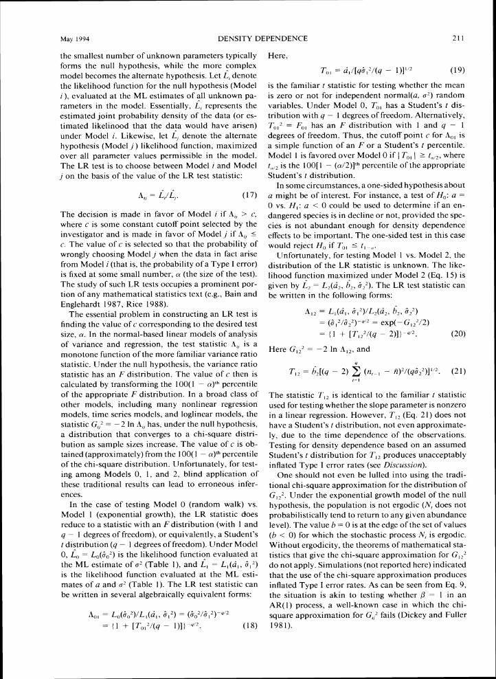
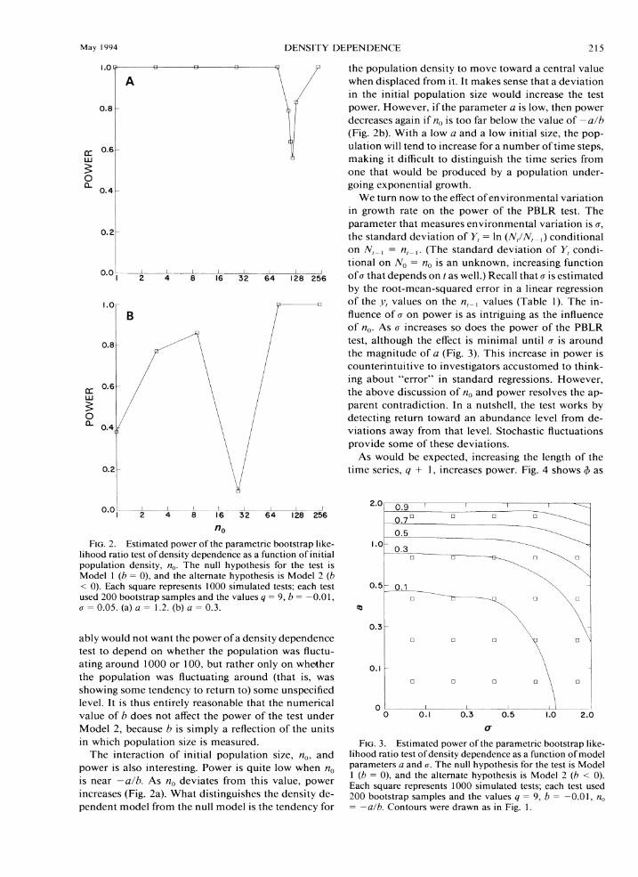
FIG.4. Estimated power of the parametric bootstrap like-lihood ratio test ofdensity dependence as a function of sample size, q (number of one-step transitions in the time series). The null hypothesis for the test is Model I (h = 0). Each symbol represents I000 simulated tests; each test used 200 bootstrap samples and the values h = -0.01, u = 0.05. n,, = a / h .
a function of q for a spectrum of a values ranging from 0.3 to 1.2. All simulations in this figure had initial sizes fixed at n,, = -a/h, and thus power is a t a local min-imum. Nonetheless. power becomes quite reasonable by the time q is 16. Even time series as short as eight transitions can have a nontrivial probability of reject-ing the false null hypothesis if the rate parameter a is not small. In the figure, the two curves marked with stars portray power for a series of runs with a equal to 0.6. The solid line is for one-sided tests and the dashed line represents two-sided tests. The difference between the two types of tests in the probability of correctly rejecting the null hypothesis may be important, par-ticularly when power is modest. In the figure when q is 16, the power of the one-sided test is almost twice the power of the two-sided test. Many ofthe abundance records for natural populations are only 10-30 yr long. Power is expected to only be moderate. Thus we strong-ly recommend the use of the one-sided test.
Knowledge of a test's power is extremely useful when interpreting results. If power is low then failure to reject the null hypothesis contributes only weak evidence in favor of the null model. True power can only be quan-tified if the real parameters are known. For the density dependence test, the power can be estimated in a sta-tistically consistent fashion by substituting the empir-ically estimated parameters for the true parameters and conducting a Monte Carlo simulation such as described above. However, we suggest some caution in that such power estimates will only approximate the true power in small samples. The maximum likelihood parameter estimates under the density dependent model have a finite sample bias. While this has n o influence on the
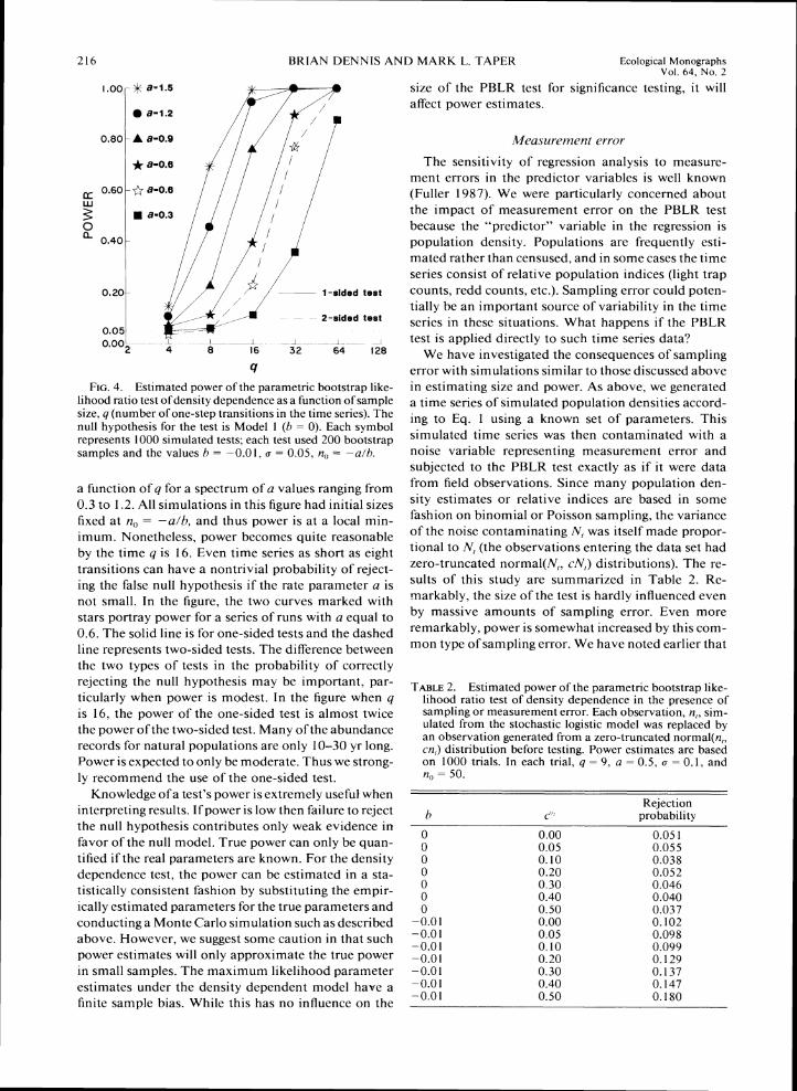
error with simulations similar to those discussed above in estimating size and power. As above, we generated a time series of simulated population densities accord-ing to Eq. 1 using a known set of parameters. This simulated time series was then contaminated with a noise variable representing measurement error and subjected to the PBLR test exactly as if it were data from field observations. Since many population den-sity estimates o r relative indices are based in some fashion on binomial o r Poisson sampling. the variance of the noise contaminating N, was itself made propor-tional to i?v; (the observations entering the data set had zero-truncated normal(hT,.cN,) distributions). The re-sults of this study are summarized in Table 2. Re-markably, the size of the test is hardly influenced even by massive amounts of sampling error. Even more remarkably. power is somewhat increased by this com-mon type of sampling error. We have noted earlier that
TABLE2. Estimated power of the parametric bootstrap like-lihood ratio test of density dependence in the presence of sampling or measurement error. Each observat~on.n,. sim-ulated from the stochastic logistic model was replaced by an observation generated from a zero-truncated normal(n,. cn,) distribution before testing. Power estimates are based on 1000 trials. In each trial. q = 9, a = 0.5, u = 0.1, and n,,= 50.

Ma) 1994 DENSITY DEPENDENCE 2 17
TABLE 3. Parametric bootstrap likelihood ratio test of density dependence for the grizzly bear population in the Yellowstone reglon. The null hypothesis for the test is Model 1 (h = O), and the alternate hypothesis is Model 2 (h < 0). Number of bootstrap samples = 8000.
Maximum likelihood parameter estimates under Model I (density independence) a , = 4.14 x 10 ': u , ' = 1.49 x l o - '
Maximum likelihood parameter estimates under Model 2 (densit) dependence) a, = 1.41 x 10 I: 15, = 2 ; 4 1 x 10 '; u L Z= 1.45 x 10 ~2
Likelihood ratio statistics5 'I.,,= 0 . 6 0 ; i,,,, = 2 . 9 : P = 0 . 7 2
* Original data consist of the yearly counts of adult females seen with cubs, from 1973-1991 (Eberhardt et al. 1986; R. R. Knight. [~rr.sonal c~ot~~ttrlctiic~ation). Values listed here for .2; are calculated from the original data as a 3-yr moving sum (sum of 1973. 1974. and 1975 counts. sum of 1974. 1975, and 1976 counts, etc.).
S: Likelihood ratio test statistic (Eq. 21). estimated fifth percentile of the test statistic distribution under Model I . and estimated P value for the test.
deviations increase the power of this test. Apparently, these deviations d o not even have to be entirely real.
We present. in this section. several worked examples of the PBLR test of density dependence. Numerous examples of density dependence testing in the literature have involved insect populations. T o the scarce supply of large mammal examples in the density dependence debate, we add a few more (Tables 3-5). Fowler (1 984, 1987) has given additional information and insights about density dependence in large mammals. In this section we also analyze 16 insect data sets assembled by den Boer and Reddingius (1 989) in order to compare results of the PBLR test to earlier published results.
The grizzly bear (C'rsus arctos horrihilis) population of the greater Yellowstone ecosystem shows no evi- dence of density dependence in time series abundance data (Table 3). The data (Table 3) consist of a 3-yr running sum of adult females seen with cubs. An adult female produces cubs on average every 3 yr, so the 3-yr running sum of this relatively visible component of the population represents an estimate of the minimum number of adult females in the population (see Knight and Eberhardt 1984. 1985. Eberhardt et al. 1986, and Dennis et al. 199 1 for discussion). Table 3 reflects the counts from 1973 through 199 1 (Eberhardt et al. 1986, R. R. Knight, personal cornfi~unication). Dennis et al. (1 99 1) found increased variability in the data after 197 1. possibly related to the garbage d u m p closures in 1970- 1971 or to institution of new aerial survey methods. The outcome of the density dependence test suggests that the population has not yet reached carrying ca- pacity, that is, the time series gives n o reason to favor Model 2 over Model 1.
Results of model diagnostic procedures for the griz- zly data are mixed. The residuals from both models are normally distributed, according to the Lin-Mu- dholkar test (Model 1: LM = -0.28. P = .78; Model 2: LM = -0.78, P = -.43; see Tong 1990:324). How- ever, the residuals from both models have some au- tocorrelation, according to standard tests with the first- and second-order sample autocorrelation statistics
(Model 1: G;,= -2.73, P = .0064; Gb2= 1.77, P= .077; Model 2: f i b , = -2.21, P = ,027; Gj2= 1.71, P = .088; see Tong 1990:324). While the properties of these or other white noise tests have not been inves- tigated for the residuals of Model 2, the results suggest that the grizzly female population has a higher order autocorrelation structure not accounted for by either Model 1 o r Model 2. Oscillations from year-class im- balances in the population could cause such autocor- relation. The large variability of the population. though, gives reason for concern about its long-term viability (Dennis et al. 1991).
Two elk ( C ~ r v u s elaphus) populations in the greater Yellowstone ecosystem have noticeable density depen- dence (Tables 4 and 5). The data on the northern Yel- lowstone population (Table 4) are winter census rec- ords from Houston (1 982: 17): the data on the central valley population in Grand Teton National Park (Table 5) are from Boyce (1 989) and represent summer mark- recapture estimates
The northern Yellowstone population increased rap- idly after artificial removals from the park were ended in 1969. The population appears to have subsequently attained a stochastic equilibrium. The power of the density dependence test was enhanced because the ini- tial population was far from equilibrium (see T ~ s t val-idation). Residual plots and tests show n o outliers, no significant first- o r second-order autocorrelation, and n o significant departures from normality (Model 1 : LM = 0.91, P = .36; f i b 1 = 0.89, P = .37: f i b 2 = 1.26, P = .26; Model 2: LM = -1.08, P = .28; Gj3,=
-1.53, P = .13; f i b 2 = 0.21, P = .83; seeTong 1990: 324).
The central valley population in Grand Teton Na- tlonal Park fluctuates substantially, and the estimated P value for the test is just under .05. The Grand Teton population has a missing observation in year 1983, and so the test was conditioned on n2 , (= 1453) in addition to n,, (= 1627) (see Hypothesis fating). The second transition (1 527 to 824) is a possible outlier for both Model 1 and Model 2, with a standardized residual of -2.7 for Model 2. N o significant first- or second-order autocorrelation is evident in the first 19 consecutive

1 18 BRIAN DENNIS AND MARK L. TAPER Ecological Monographs Vol. 64, No. 2
TABLE4. Parametnc bootstrap likel~hood ratio test of density dependence for the northern Yellowstone elk population. The null hypothesis for the test is Model 1 (h = 0). and the alternate hypothesis is Model 2 (h < 0). Number of bootstrap samples = 8000.
Population size data. N,* 3171 4305 5543 728 1 8215 998 1 10 529 12 607 10 807 10 741 1 1 855 10 768
Maximum li~elihood parameter estimates under Model I (density independence)
Maximum likelihood parameter estimates under Model 2 (density dependence)
Likelihood ratio statistics5
* Data are winter census records from 1968-1979 listed by Houston (1 982). The 1977 value is an adjusted value given by Houston (1 982:23).
5 Likelihood ratio test statistic (Eq. 21), estimated fifth percentile of the test statistic distribution under Model I , and estimated P value for the test.
residuals (Model 1: mi,= -0.69, P = .49; mi, curred simply by chance? If one assumes that all 16 = -0.95, P = .34; Model 2: m;,= 0.48, P = .63; populations follow the null hypothesis model (sto-m 2= 0 . 3 2 . P = .75). With the outlier removed, chastic exponential growth), then two or more "suc- the residuals are acceptably normal (Model 1: LM = cesses" out of 16 trials is a plausible outcome when 1.95, P = .051; Model 2: LM = 1.91, P = ,056). the success probability is .05 (if U' - binomial (16,
den Boer and Reddingius (1989) used the Pollard et 0.05), then P[U' 2 21 .19). However. there is more al. (1987) randomization test to look for density de- information present in the collection of P values than pendence in 16 insect populations. Their paper pro- simply the number of them < .05. If all the populations vides a table with the original data. The randomization were realizations of the null hypothesis model. the P test d ~ d not flag a single population as density depen- values would represent 16 independent observations dent. By contrast, the PBLR test rejects density inde- from a uniform(0, 1) distribution. Then -2 In P, would pendence for two of the populations at the .05 slgnif- be an observation from a chi-square(2) distribution, icance level (Table 6). If the regression test for h < 0 and the sum of k such values would be an observation based on the Student's t distribution is used, the density from a chi-square(2k) distribution (Fisher's test; see dependent count jumps to eight (Table 6). Fisher 1958). From the P values in Table 6. we find
The den Boer and Reddingius (1 989) data illustrate that S - 2 In P, = 46.1. a value that is just below the the role of test power. The regression test is obviously 95Ih percentile of the chi-square(32) distribution (P' more powerful but is inappropriate because it is not a = .05 1). Enough of the P values in this meta-analysis size 0.05 test (see Discussion). Both the randomization are "leaning" toward the alternate hypothesis end so and the PBLR are close to size 0.05 tests. Because of as to cast doubt upon the assumption that all 16 pop- the asymptotic relative efficiency of LR tests, the PBLR ulations are realizations of the density-independent test probably represents the practical limit of power model, though one would not reject that assumption for testing b < 0 in the stochastic logistic model. Even at a strict .05 significance level. though the power can exceed that of the randomization test by 50% (see D~scussion). the basic thrust of den DISCUSSION
Boer and Reddingius' results remains intact. If there The PBLR test can easily be adapted, if desired, to is density dependence in these 16 populations. it is testing for density dependence under the Gompertz difficult to detect from time series data alone. model (Eqs. 7 and 8). The modification would use x,
Could the two density dependent cases have oc- values in place of n, values in the parameter estimates
TABLE5. Parametric bootstrap likelihood ratio test of density dependence for the elk population in the central valley of Grand Teton National Park. The null hypothesis for the test is Model 1 (h = 0), and the alternate hypothesis for the test IS Model 2 (h < 0). Number of bootstrap samples = 8000.
Population size data, N,* 1627 1527 824 891 1140 1322 1431 1733 1131 1611 1644 1991 1762 1076 1442 I800 1667 1558 1396 1753 . . . 1453 1804
Maximum likelihood parameter estimates under Model I (density independence) a , = 1.45 x 10 2 : 8,:= 6.85 x
Maximum likelihood parameter estimates under Model 2 (density dependence) 6, = 7.31 x 10 I; h, = -4.93 x l o 4 ;6:' = 4.65 x 1 0 2
Likelihood ratio statistics8 T , , = 2 . 9 2 ; f,,, = -2.88; P = 0.044
* Data are simmer mark-recapture population estimates from 1963-1985 (1983 missing) listed by Boyce (1989). Likelihood ratio test statistic (Eq. 21), estimated fifth percentile of the test statistic distribution under Model I, and
estimated P value for the test.

~ - ~ ~ ~ ~ ~
Ma) 1994 DENSITY DEPENDENCE 2 19
(Table 1) for the alternate hypothesis model. The re- suiting test is essentially the modification of vickery and Nudd's test that was sug-gested by Pollard et al. (1 987). The test procedure is i t h e w i s e identical to the test we have proposed. Mountford (1988) employed such a G ~ PBLR test using Model 0 (random walk) as the null hypothesis.
Reddingius (1 97 1) recognized the theoretical deslr- ability of LR tests, and he developed a small table of critical values for the Gompertz-based LR statistic us- ing Monte Carlo simulation. In practice. the investi-
gator must estimate parameters from the data before referring to the table. Use of Reddingius' table thus is quite similar to conducting a PBLR test for Gompertz- type density dependence.
Many subsequent investigators have taken (implic- itly o r explicitly) the Gompertz model as the alternate hypothesis in density dependence tests, but have used different test statistics (Bulmer 1975. Royama 1977, Slade 1977, Vickery and Nudds 1984, 1991, Gaston and Lawton 1987, Pollard et al. 1987, den Boer and Reddingius 1989. Reddingius and den Boer 1989, den Boer 1990, Holyoak and Lawton 1992. Woiwod and Hanski 1992). Crowley ( 1992) modified the Gompertz to include sampling variability. The statistics include the sample correlation of the y,'s and s ,,'s (Pollard et al. 1987), the slopes of principal and reduced major axes (Slade 1977), the reciprocal of von Neumann's ratio (Bulmer 1975). and the number of times that the one-step transitions have moved toward (or away) from a given abundance level (Crowley 1992).
Of the tests studied by these investigators, the ran- domization test of Pollard et al. (1987) based on the sample correlation coefficient appears the most pow- erful (Vickery and Nudds 199 1. Crowley 1992). This is not surprising: the LR statistic for testing whether h = 0 in the Gompertz model (or in the logistic model) is a monotone function of the squared sample corre- lation coefficient:
Here R is the sample correlation coefficient of the 11,'s and x, ,'s (or n, ,'s if the test is adapted to the logistic model given by Eq. 1). The randomization procedure proposed by Pollard et al. (1987) estimates the distri- bution of R or R2 by taking random permutations of the 1:'s to construct new time series data sets. A new value of R2 is obtained from each set. This is essentially a form of nonparametric bootstrapping. However. the resulting estimate of the distribution of R2(or R, or A) under the null hypothesis does not make use of the sufficient statistics a and C 2 , and therefore does not make the most efficient use of the data ("sufficient statistics" contain all the information about model pa- rameters that is present in the data: see Rice 1988).
Our simulations reveal that the randomization test of Pollard et al. (1987) is considerably less powerful
TABLE6. Results of two density dependence tests performed on 16 insect data sets listed by den Boer and Reddingius (1989). Shown are the values of the likelihood ratio test statistic (T ,>) ,the number ofone-step transition~(q), the P values estimated bv ~arametr ic boots t ra~~incl(P). and the Pvalues resulting fiom a Student's t distribution with q - 2 degrees of freedom (P,,,,,,,). The null hypothesis is Model ~ ~ ~ ~ 1 (b = 0), and the alternate hypothesis is Model 2 (b < 0). Order of entry corresponds to order in den Boer and Red- dingius' (1989) ~ a b l ~ 1
T12 9 P Pbtudcnt
-1.84 18 .243 ,042 -2.54 18 .089 .0 l l -3 14 14 .033 .004 -3.07 14 ,033 .005 -1.51 13 .436 ,080 -2.15 13 ,154 ,027-2.52 12 ,095 .0 15 -0.9 1 2 8 ,776 .I85 - 1.45 18 ,349 ,083 - 1.29 19 ,457 .I07 -1.61 14 ,378 .067 -2.07 13 ,198 .03 1 72.17 I I .999 .97 1
than the PBLR test when the data are generated from the stochastic logistic model given by Eq. 1 (Table 7). The parametric test attains as much as a 50% increase in power over a range of parameter values. Even if the randomization test is adapted to the logistic model. by using n , ,'s instead of s ,,'s in Eq. 27, the power levels of the parametric test are not approached (Table 7).
There might be some nonparametric benefits in terms of robustness of the randomization test, though such benefits have not been assessed. The stochastic logistic (Eq. 1) that we have assumed as the alternate hypoth- esis is a fairly general model that can describe many situations. Possible modifications of the model for studying robustness of tests might include use of a heavy-tailed distribution for the Z,'s instead of the normal distribution, o r allowing the Z,'s to be auto- correlated. Few abundance data sets have more than 30 observations, however, and it is likely that the full benefits of nonparametric approaches (which depend heavily on large-sample consistency theorems) to den- sity dependence testing will not be realized in practice.
Use of the Gompertz stochastic model in and of itself could involve a loss of power. Detecting growth-rate feedback that is proportional to In N, instead of N,will likely require data covering wider ranges of abundance. As noted before, a PBLR test can be constructed for the Gompertz model; such a test would represent the practical limit of power that can be attained under that model. If this PBLR-Gompertz test is performed on data arising from a stochastic logistic. the size of the test remains -0.05. but a detectable loss of power en- sues (Table 7). The difference in power between the PBLR-logistic and the PBLR-Gompertz quantifies the

220 BRIAN DENNIS AND MARK L. TAPER Ecological Monographs Val. 64. No. 2
TABLE7. Estimated sizes and powers of various one-sided density dependence tests, when data arise from the stochastic logistic model.* Tests are the parametric bootstrap likelihood ratio (PBLR) tests based on the stochastic logistic and the stochastic Gompertz and randomization tests based on the stochastic logistic and stochastic Gompertz. All tests were conducted at a nominal significance level of .05 and used 200 bootstrap or randomized samples where appropriate. Each estimate was obtained from 1000 trials. For all tests. q = 9.
PBLR PBLR Randomization Randomization h n,, u a (logstic) (Gompertz) (logistic) (Gompertz)
0 130 0.25 0.5 0.039 0.053 0.041 0.039 0 100 0.25 I .0 0.05 1 0.039 0.052 0.052 0 100 0.25 1.5 0.045 0.060 0.050 0.05 1 0 100 0.50 0.5 0.052 0.029 0.038 0.050 0 100 0.50 I .0 0.050 0.048 0.048 0.044 0 100 0.50 1.5 0.046 0.045 0.046 0.039 0 100 0.75 0.5 0.04 1 0.045 0.035 0.042 0 100 0.75 1 .0 0.049 0.045 0.063 0.059 0 100 0.75 1.5 0.056 0.047 0.052 0.044 0 100 1.OO 0.5 0.046 0.055 0.040 0.049 0 100 1 .OO 1 .0 0.065 0.050 0.043 0.042 0 100 1 .OO 1.5 0.054 0.040 0.039 0.052
-0.01 -alh 0.25 0.5 0.104 0.101 0.086 0.084 -0.01 a l h 0.25 I .0 0.362 0.354 0.304 0.290 -0.01 a l h 0.25 1.5 0.759 0.742 0.699 0.692 0 . 0 1 -a/h 0.50 0.5 0.152 0.1 12 0.104 0.092 0 . 0 1 -a/h 0.50 1.0 0.424 0.399 0.322 0.270 0 . 0 I -a/h 0.50 1.5 0.807 0.608 0.682 0.665 -0.01 a l h 0.75 0.5 0.191 0.121 0.106 0.103 0 . 0 I a / h 0.75 1.0 0.494 0.269 0.333 0.250 0 . 0 1 a l h 0.75 1.5 0.775 0.458 0.675 0.42 1 0 . 0 1 -alh 1 .OO 0.5 0.237 0.131 0.107 0.095 0 . 0 1 -alh 1.OO I .0 0.562 0.220 0.336 0.188 -0.01 a l h 1.OO 1.5 0.788 0.298 0.629 0.308
* The model is Y, = a t hN, , + mZ,. where N, is population abundance at time t , Y,= In(N,/N,,,), Z, - normal(0, I). and t = I . 2 , . . . , q.
intrinsic effect of looking for density dependence with logistic model, particularly with modifications for sec- a model of log-density dependence. ond-order lags (Eq. 6), have reported pervasive evi-
Of course, one could just as easily take the Gompertz dence of density dependence (Turchin 1990. Turchin as the "true" model in the simulations. The logistic. et al. 199 1, Benyman 199 la). Some of these results though, is fundamentally a nonlinear dynamic model are probably influenced by the properties of the re-and possesses a wider range of dynamic behaviors (such gression-based statistical testing methods they used. As as limit cycles and chaos). The Gompertz is funda- we have noted, the t and Fstatistics for testing whether mentally a linear dynamic model (see Eq. 9) and there- slope parameters are zero in Eq. 6 d o not have t or F fore has a restricted repertoire of dynamic behaviors. distributions. Our simulations indicate that the Type The logistic would seem a more flexible choice for I error rates in one-sided tests of first- o r second-order modeling the dynamic behavior of natural populations. lags using Student's t distributions are markedly in- and we have therefore centered our investigations flated over the nominal rate of 0.05 (Table 8). Users around statistical properties arising from the logistic. of such tests will find density dependence too often
Some investigators using Gompertz-based methods when it in fact is weak or absent. Extensions of the t have concluded that density dependence is frequently and Ftests to multispecies versions of the logistic (Ber- weak and not as widely prevalent as theoretical ecol- ryman 1991b) must be called into question as well, ogists might expect (den Boer and Reddingius 1989, until such tests receive further study. In addition. the den Boer 1990). Without extensive logistic-Gompertz regression-based, two-sided test for a first-order lag has model evaluations and analyses using many data sets, inflated Type I error rates for some parameter values it is not clear whether their results arise from nature (Table 8). The regression-based, two-sided test for a o r from increased Type I 1 error rates inherent in the second-order lag appears to possess reasonable Type I Gompertz-based statistical methods. The low power error rates (Table 8). It is noteworthy that the inves- of such methods has been acknowledged (Vickery and tigators have tended to use the two-sided regression Nudds 199 l), though not explained. We speculate that test for second-order lags. Thus, their results concern- searching for density dependence with a model of log- ing the prevalence of second-order lags might hold up density dependence might be akin to trying to photo- when the data are analyzed with techniques that have graph a distant bird with a wide-angle instead of a received thorough evaluation. telephoto lens. The PBLR procedure can be adapted to test for sec-
On the other hand, investigators using the stochastic ond-order lags. Such a test provides a check on the
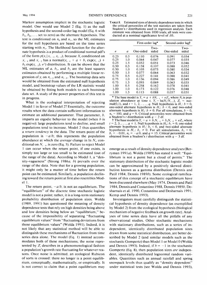
Ma) 1994 DENSITY DEPENDENCE 22 1
Markov assumption implicit in the stochastic logistic model. One would use Model 2 (Eq. 1) as the null hypothesis and the second-order lag model (Eq. 6 with h,. h,. . . . set to zero) as the alternate hypothesis. The test is conditioned on n,, and n , , so the M L estimates for the null hypothesis are based on the time series starting with n , . The likelihood function for the alter- nate hypothesis is a product of conditional normal pdf s of the form p(.v, I .v , ,,s,-,),because X, conditioned on s, , and s,,has a n o r m a l ( s , , + a + b, exp(x-, ,) + bz e x p ( s , , ) , o') distribution. It can be shown that the ML estimates of a , h , , and h, are the least squares estimates obtained by performing a multiple linear re- gression of J: on n, , and n,-,. The bootstrap data sets would be obtained from the estimated null hypothesis model, and bootstrap values of the LR statistic would be obtained by fitting both models to each bootstrap data set. A study of the power properties of this test is in progress.
What is the ecological interpretation of rejecting Model 1 in favor of Model 2? Essentially, the outcome results when the data contain sufficient information to estimate an additional parameter, That b, imparts an ergodic behavior to the model (when h is negative): large populations tend to decline, and small popu~ations tend to increase. ~ ~2 thus quantifies d ~ l a return tendency in the data. The return point of the population is -a/h; this represents the population abundance at which the average change in In N,.con-ditional on Nli, , , is zero (Eq. 5). Failure to reject Model 1 can occur when the return point. if one exists, is simply too large or too small to be estimated (out of the range of the data). According to Model 1, a "den- sity-vagueness" (Strong 1986a, h) prevails over the range of the data. Note that for a growing population, it might only be a matter of time before the return point can be estimated. Similarly, a population declin- ing toward the return point a t first also resembles Mod- el 1.
The return point, -a/b, is not a n equilibrium. The "equilibrium" of the discrete time stochastic logistic model is not a point; rather, it is a long-term stationary probability distribution of population sizes. Wolda (1 989. 199 1) has questioned the meaning of density dependence tests that rely on high densities being above and low densities being below an "equilibrium," be-cause of the impossibility of separating "fluctuating equilibrium values" from "fluctuating deviations from those equilibrium values" (Wolda 199 1). Indeed, it is not likely that any statistical method will be able to distinguish these mechanisms of fluctuation from time series data alone. The model (Eq. 1) instead accom- modates both of these mechanisms; the noise repre- sented by Z, describes in a phenomenological fashion a population's growth rate fluctuating for whatever rea- sons. Once noise is admitted, an ecological Rubicon of sorts is crossed: there no longer is a point equilib- rium, conceptually, mathematically, o r empirically. It is not correct to claim that a point equilibrium may
TABLE8. Estimated sizes ofdensity dependence tests in which the critical percentiles of the test statistics are taken from Student's t distributions used in regression analysis. Each estimate was obtained from 1000 trials; all tests were con- ducted at a nominal significance level of .05.
First-order lag* Second-order lag?
Two- Two-u a One-sided sided One-sided sided
0.25 0.5 0.1 10 0.076 0.091 0.054 0.25 1.0 0.064 0.047 0.077 0.035 0.25 1.5 0.052 0.05 1 0.073 0.046 0.50 0.5 0.158 0.107 0.088 0.052 0.50 1.0 0.105 0.075 0.080 0.034 0.50 1.5 0.077 0.064 0.063 0.032 0.75 0.5 0.227 0.141 0.088 0.041 0.75 1.0 0.136 0.094 0.086 0.049 0.75 1.5 0.095 0.069 0.063 0.035 1.00 0.5 0.258 0.162 0.078 0.041 1.00 1.0 0.173 0.122 0.076 0.048 1.00 1.5 0.1 15 0.088 0.057 0.031
* The base model is Y, = a + hhr ,, + uZ,.where N, is pop- ulation abundance at time t , Y, = ln(A',IN,-,), Z, - nor-mal(O,l), and t = 1. 2. . . . , q. Null hypothesis is H I : h = 0. one-sided alternate hv~othesis is H,: h < 0. and two-sided alternate hypothesis is^^: h # 0. F& all simulations, h = 0. no = 100, and q = 9. Critical percentiles were obtained from a Student's r distribution with q - 2 df.
t Thebasemodel is y, = a + h , ~ , - , + u ~ , ,+ b,hr, where r = 2, 3. . . . , q + I . Null hypothesis is H,,:h, = 0, one-sided alternate hypothesis is H I : h1 < 0. and two-sided alternate hypothesis is H I : h2 # 0. For all simulations. h, = 0. hl = -0.01, = a , b , and = 5. critical percentiles were obtained from a Student's r distribution with q 3 df. -
emerge as a result of density dependence analyses (Ber- ryman 199 1 a). Wolda (1 989) has stated it well: "Equi- librium is not a point but a cloud of points." The stationary distribution of the stochastic logistic model can be approximated by a positively skewed distri- bution known as a gamma distribution (Dennis and Patil 1984, Dennis 19896). Some ecological ramifica- tions of this concept of a stochastic equilibrium have been discussed elsewhere (May 1974, Dennis and Patil 1984. Dennis and Costantino 1988. Dennis 19896, De- sharnais et al. 1990, Costantino and Desharnais 199 1, Kemp and Dennis 1993).
Investigators must carefully distinguish the statisti- cal hypothesis of density dependence (as exemplified by Model 2) from the ecological hypothesis (biological mechanism of negative feedback on growth rate). Anal- yses of time series data have all the pitfalls of any observational studies. Other stochastic mechanisms with stationary distributions. such as a series of in- dependent, identically distributed population sizes drawn from some statistical distribution, are better de- scribed by Model 2 (and similar models such as the stochastic Gompertz) than Model 1 or Model 0 (Wolda and Dennis 1993). Indeed. if h = - 1 in the stochastic Gompertz (Eq. 8), then population sizes arc> indepen- dent, identically distributed lognormal random vari- ables. Quantities such as annual rainfall and spring snowpack levels thus qualify as "density dependent" under statistical tests (see Wolda and Dennis 1993).
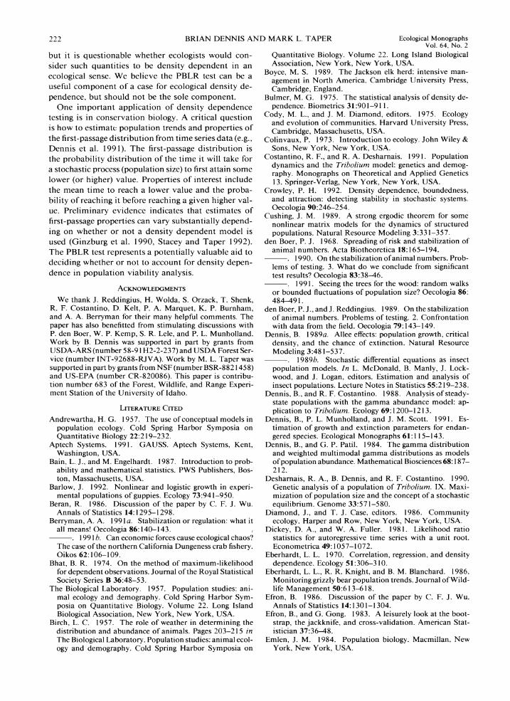
979 --- BRIAN DENNIS AX ID MARK L. TAPER Ecolog~cal Monographs
but it is questionable whether ecologists would con-sider such quantltles to be density dependent in an ecological sense. We believe the PBLR test can be a useful component of a case for ecological density de- pendence. but should not be the sole component.
One important application of density dependence testing is in conservation biology. A critical question is how to estimate population trends and properties of the first-passage distribution from time series data (e.g., Dennis et al. 1991). The first-passage distribution is the probability distribut~on of the time it will take for a stochastic process (population size) to first attain some lower (or higher) value. Properties of Interest include the mean time to reach a lower value and the proba- bility of reaching it before reaching a given hlgher val- ue. Preliminary evidence indicates that estimates of first-passage properties can vary substantially depend- ing on whether o r not a density dependent model is used (Ginzburg et al. 1990, Stacey and Taper 1992). The PBLR test represents a potentially valuable aid to deciding whether o r not to account for density depen- dence in population viability analysis.
ACKNOWLEDGMENTS
We thank J. Reddingius, H. Wolda, S. Orzack, T. Shenk, R. F. Costantino, D. Kelt, P. A. Marquet, K. P. Burnham, and A. A. Benyman for their many helpful comments. The paper has also benefitted from stimulating discussions with P. den Boer, W. P. Kemp. S. R. Lele, and P. L. Munholland. Work by B. Dennis was supported in part by grants from USDA-ARS (number 58-9 1H2-2-237) and USDA Forest Ser- vice (number INT-92688-RJVA). U'ork by M. L. Taper was supported in part by grants from NSF (number BSR-882 1458) and US-EPA (number CR-820086). This paper is contribu- tion number 683 of the Forest, Wildlife. and Range Experi- ment Station of the University of Idaho.
Andrewartha, H. G. 1957. The use of conceptual models in population ecology. Cold Spring Harbor Symposia on Quantitative Biology 22.2 19-232.
Aptech Systems. 199 1. GAUSS. Aptech Systems, Kent, Washington. USA.
Bain, L. J.. and M. Engelhardt. 1987. Introduction to prob- ability and mathematical statistics. PWS Publishers, Bos- ton, Massachusetts, USA.
Barlow. J. 1992. Nonlinear and logistic growth in experi- mental populations of guppies. Ecology 73:941-950.
Beran, R. 1986. Discussion of the paper by C. F. J . Wu. Annals of Statistics 14: 1295-1 298.
Berryman, A. A. 1991a. Stabilization or regulation: what it all means! Oecologia 86: 140- 143.
-. 199 I h. Can economic forces cause ecological chaos? The case of the northern California Dungeness crab fishery. Oikos 62: 106-109.
Bhat, B. R. 1974. On the method of maximum-likelihood for dependent observations. Journal of the Royal Statistical Society Series B 36:48-53.
The Biological Laboratory. 1957. Population studies: ani- mal ecology and demography. Cold Spring Harbor Sym- posia on Quantitative Biology. Volume 22. Long Island Biological Association, New York, New York. USA.
Birch, L. C. 1957. The role of weather in determining the distribution and abundance of animals. Pages 203-2 15 in The Biological Laboratory. Population studies: animal ecol- ogy and demography. Cold Spring Harbor Symposia on
Vol. 64. No. 2
Quantitative Biology. Volume 22. Long Island Biological Association, New York, New York, USA.
Boyce, M. S. 1989. The Jackson elk herd: intensive man- agement in North America. Cambridge University Press, Cambridge. England.
Bulmer, M. G. 1975. The statistical analysis of density de- pendence. Biometries 31:90 1-9 1 I.
Cody, M. L., and J. M. Diamond. editors. 1975. Ecology and evolution of communities. Harvard University Press, Cambridge, Massachusetts. USA.
Colinvaux, P. 1973. Introduction to ecology. John Wiley & Sons. New York. New York, USA.
Costantino, R. F., and R. A. Desharnais. 1991 . Population dynamics and the Trlholium model: genetics and demog- raphy. Monographs on Theoretical and Applied Genetics 13. Springer-Verlag. New York. New York, USA.
Crowley, P. H. 1992. Density dependence, boundedness, and attraction: detecting stability in stochastic systems. Oecologia 90:246-254.
Cushing, J. M. 1989. A strong ergodic theorem for some nonlinear matrix models for the dynamics of structured populations. Natural Resource Modeling 3:33 1-357.
den Boer, P. J. 1968. Spreading of risk and stabilization of animal numbers. Acta Biotheoretica 18: 165-1 94.
. 1990. On the stabilization ofanimal numbers. Prob- lems of testing. 3. What do we conclude from significant test results? Oecologia 83:38--46.
. 199 1. Seeing the trees for the wood: random walks or bounded fluctuations of population size? Oecologia 86: 484-49 1.
den Boer, P. J., and J. Reddingius. 1989. On the stabilization of animal numbers. Problems of testing. 2. Confrontation with data from the field. Oecologia 79: 143-149.
Dennis, B. 1 9 8 9 ~ . Allee effects: population growth, critical density, and the chance of extinction. Natural Resource Modeling 3:48 1-537.
. 19896. Stochastic differential equations as insect population models. In L. McDonald, B. Manly, J. Lock-wood, and J. Logan, editors. Estimation and analysis of insect populations. Lecture Notes in Statistics 55:2 19-238.
Dennis, B., and R. F. Costantino. 1988. Analysis of steady- state populations with the gamma abundance model: ap- plication to Triholium. Ecology 69: 1200-1 2 13.
Dennis. B., P. L. Munholland, and J. M. Scott. 1991. Es-timation of growth and extinction parameters for endan- gered species. Ecological Monographs 61: 1 15-1 43.
Dennis, B., and G. P. Patil. 1984. The gamma distribution and weighted multimodal gamma distributions as models of population abundance. Mathematical Biosciences 68: 187- 212.
Desharnais. R. A.. B. Dennis. and R. F. Costantino. 1990. Genetic analysis of a population of Triholiurn. IX. Maxi- mization of population size and the concept of a stochastic equilibrium. Genome 33:57 1-580.
Diamond, J. , and T. J. Case, editors. 1986. Community ecology. Harper and Row, New York. New York, USA.
Dickey, D. A,, and W. A. Fuller. 1981. Likelihood ratio statistics for autoregressive time series with a unit root. Econometrica 49: 1057-1 072.
Eberhardt, L. L. 1970. Correlation, regression, and density dependence. Ecology 51:306-3 10.
Eberhardt, L. L., R. R. Knight, and B. M. Blanchard. 1986. Monitoring grizzly bear population trends. Journal of Wild- life Management 50:6 13-6 18.
Efron, B. 1986. Discussion of the paper by C. F. J. Wu. Annals of Statistics 14: 130 1-1 304.
Efron, B., and G. Gong. 1983. A leisurely look at the boot- strap, the jackknife, and cross-validation. American Stat- istician 37:36-48.
Emlen, J. M. 1984. Population biology. Macmillan. New York. New York, USA.
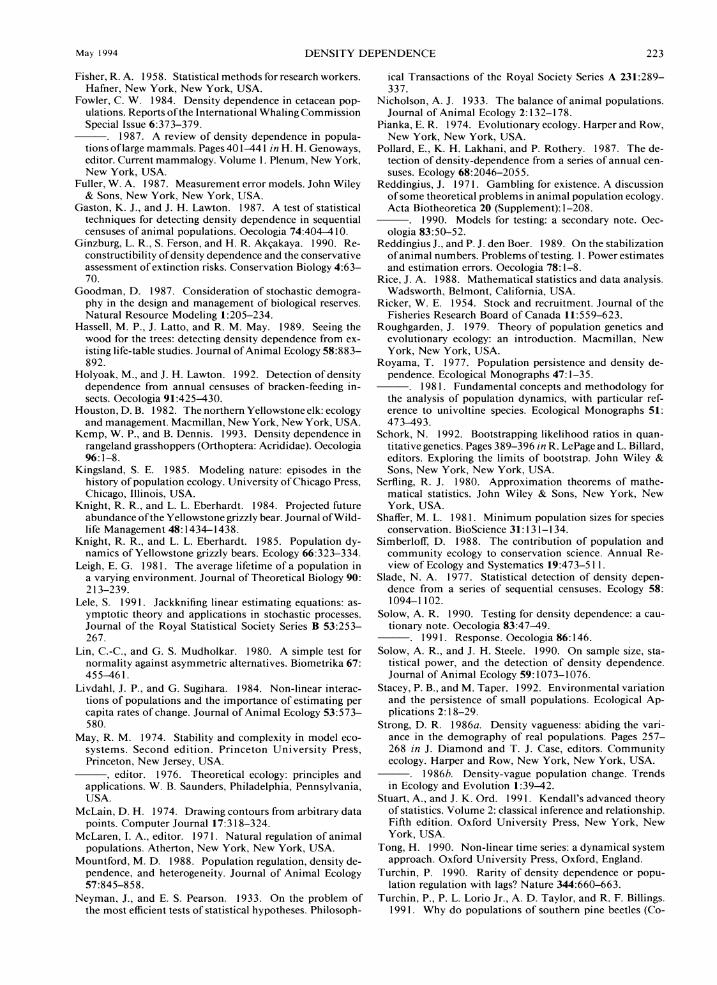
May 1994 DENSITY DEPENDENCE 223
Fisher, R. A. 1958. Statistical methods for research workers. Hafner, New York, New York, USA.
Fowler, C. W. 1984. Density dependence in cetacean pop- ulations. Reports ofthe International Whaling Commission Special Issue 6:373-379.
-. 1987. A review of density dependence in popula- tions of large mammals. Pages 40 1-44 1 in H. H. Genoways, editor. Current mammalogy. Volume 1. Plenum. New York. New York, USA.
Fuller, W. A. 1987. Measurement error models. John Wiley & Sons, New York, New York, USA.
Gaston. K. J.. and J. H. Lawton. 1987. A test of statistical techniques for detecting density dependence in sequential censuses of animal populations. Oecologia 74:404-4 10.
Ginzburg, L. R., S. Ferson. and H. R. Akpkaya. 1990. Re- constructibility of density dependence and the conservative assessment of extinction risks. Conservation Biology 4:63- 70.
Goodman, D. 1987. Consideration of stochastic demogra- phy in the design and management of biological reserves. Natural Resource Modeling 1:205-234.
Hassell, M. P.. J. Latto. and R. M. May. 1989. Seeing the wood for the trees: detecting density dependence from ex- isting life-table studies. Journal of Animal Ecology 58:883- 892.
Holyoak. M., and J. H. Lawton. 1992. Detection ofdensity dependence from annual censuses of bracken-feeding in- sects. Oecologia 91:425--430.
Houston, D. B. 1982. The northern Yellowstoneelk: ecology and management. Macmillan, New York, New York. USA.
Kemp, W. P.. and B. Dennis. 1993. Density dependence in rangeland grasshoppers (Orthoptera: Acrididae). Oecologia 96: 1-8.
Kingsland, S. E. 1985. Modeling nature: episodes in the history of population ecology. University of Chicago Press, Ch~cago. Illinois. USA.
Knight, R. R., and L. L. Eberhardt. 1984. Projected future abundance ofthe Yellowstone grizzly bear. Journal of Wild- life Management 48: 1434-1 438.
Knight, R. R., and L. L. Eberhardt. 1985. Population dy- namics of Yellowstone grizzly bears. Ecology 66:323-334.
Leigh. E. G. 198 1. The average lifetime of a population in a varying environment. Journal of Theoretical Biology 90: 2 13-239.
Lele. S. 199 1. Jackknifing linear estimating equations: as- ymptotic theory and applications in stochastic processes. Journal of the Royal Statistical Society Series B 53:253-267.
Lin, C.-C., and G. S. Mudholkar. 1980. A simple test for normality against asymmetric alternatives. Biometrika 67: 455-46 1.
Livdahl, J. P., and G. Sugihara. 1984. Non-linear interac- tions of populations and the importance of estimating per capita rates of change. Journal of Animal Ecology 53:573- 580.
May, R. M. 1974. Stability and complexity in model eco- systems. Second edition. Princeton University Press. Princeton, New Jersey, USA.
, editor. 1976. Theoretical ecology: principles and applications. W. B. Saunders, Philadelphia, Pennsylvania, USA.
McLain. D. H. 1974. Drawing contours from arbitrary data points. Computer Journal 17:3 18-324.
McLaren. I. A.. editor. 197 1. Natural regulation of animal populations. Atherton, New York. New York, USA.
Mountford, M. D. 1988. Population regulation, density de- pendence, and heterogeneity. Journal of Animal Ecology 571845-858.
Neyman, J., and E. S. Pearson. 1933. On the problem of the most efficient tests of statistical hypotheses. Philosoph-
ical Transactions of the Royal Society Series A 231:289-337.
Nicholson. A. J. 1933. The balance of animal populations. Journal of Animal Ecology 2: 132-1 78.
Pianka, E. R. 1974. Evolutionary ecology. Harper and Row, New York, New York. USA.
Pollard, E., K. H. Lakhani, and P. Rothery. 1987. The de- tection of density-dependence from a series of annual cen- suses. Ecology 68:2046-2055.
Reddingius, J. 197 1. Gambling for existence. A discussion of some theoretical problems in animal population ecology. Acta Biotheoretica 20 (Supplement): 1-208.
. 1990. Models for testing: a secondary note. Oec- ologia 83:50-52.
Reddingius J., and P. J. den Boer. 1989. On the stabilization of animal numbers. Problems of testing. 1. Power estimates and estimation errors. Oecologia 78: 1-8.
Rice. J. A. 1988. Mathematical statistics and data analysis. Wadsworth. Belmont. California, USA.
Ricker, W. E. 1954. Stock and recruitment. Journal of the Fisheries Research Board of Canada 11:559-623.
Roughgarden, J. 1979. Theory of population genetics and evolutionary ecology: an introduction. Macmillan. New York, New York, USA.
Royama, T. 1977. Population persistence and density de- pendence. Ecological Monographs 47: 1-35.
. 198 1. Fundamental concepts and methodology for the analysis of population dynamics, with particular ref- erence to univoltine species. Ecological Monographs 51: 473-493.
Schork, N. 1992. Bootstrapping likelihood ratios in quan- titativegenetics. Pages 389-396 In R. LePage and L. Billard, editors. Exploring the limits of bootstrap. John Wiley & Sons, New York, New York, USA.
Serfling, R. J. 1980. Approximation theorems of mathe- matical statistics. John Wiley & Sons. New York, New York, USA.
Shaffer, M. L. 198 1. Minimum population sizes for species conservation. BioScience 31: 13 1-1 34.
Simberloff, D. 1988. The contribution of population and community ecology to conservation science. Annual Re- view of Ecology and Systematics 19:473-5 11.
Slade, N. A. 1977. Statistical detection of density depen- dence from a series of sequential censuses. Ecology 58: 1094-1 102.
Solow, A. R. 1990. Testing for density dependence: a cau- tionary note. Oecologia 83:47-49.
. 199 1. Response. Oecologia 86: 146. Solow. A. R.. and J. H. Steele. 1990. On sample size, sta-
tistical power, and the detection of density dependence. Journal of Animal Ecology 59: 1073-1076.
Stacey. P. B., and M. Taper. 1992. Environmental variation and the persistence of small populations. Ecological Ap- plications 2: 18-29.
Strong, D. R. 1986a. Density vagueness: abiding the vari- ance in the demography of real populations. Pages 257- 268 in J. Diamond and T. J. Case. editors. Community ecology. Harper and Row. New York, New York, USA.
. 19866. Density-vague population change. Trends in Ecology and Evolution 1:39-42.
Stuart, A,. and J. K. Ord. 199 1. Kendall's advanced theory of statistics. Volume 2: classical inference and relationship. Fifth edition. Oxford University Press, New York, New York, USA.
Tong, H. 1990. Non-linear time series: a dynamical system approach. Oxford University Press, Oxford, England.
Turchin, P. 1990. Rarity of density dependence or popu- lation regulation with lags? Nature 344:660-663.
Turchin, P.. P. L. Lorio Jr.. A. D. Taylor, and R. F. Billings. 199 1. Why do populations of southern pine beetles (Co-

BRIAN DENNIS AND MARK L. TAPER Ecological Monographs Vol. 64. No. 2
leoptera: Scolytidae) fluctuate? Environmental Entomology 20:40 11109.
Turchin. P., and A. D. Taylor. 1992. Complex dynamics in ecological time series. Ecology 73:289-305.
Vickery. W. L.. and T. D. Nudds. 1984. Detection of den- sity-dependent effects in annual duck censuses. Ecology 65: 96-104.
Vickery, W. L., and T. D. Nudds. 199 1. Testing for density- de~endenteffects in secluential censuses. Oecologia 85.4 19- 423.
Wissel, C., and S. Stocker. 199 1. Extinction of populations by random influences. Theoretical Population Biology 39: 3 15-328.
Woiwod, I. P., and I. Hanski. 1992. Patterns of density dependence in moths and aphids. Journal of Animal Ecol- ogy 61:6 19-629.
Wolda. H. 1989. The equilibrium concept and density de- pendence tests. What does it all mean? Oecologia 81:430- 432.
-. 199 1. The usefulness of the equilibrium concept in population dynamics. A reply to Berryman. Oecologia 86: 144-145.
Wolda, H., and B. Dennis. 1993. Density dependence tests. are they? Oecologia 95:58 1-59 1 .